
Submitted:
15 August 2026
Posted:
17 August 2026
You are already at the latest version
Abstract
Survival analysis has been widely used to understand the etiology of chronic diseases. However, traditional survival analysis models only a single endpoint, whereas the development of chronic diseases is a multi-state process. In this review, we examine the connections among logistic regression, the Cox model, competing risk models, and multi-state models in estimating hazards and survival risks, with findings summarized in three aspects. First, logistic regression and the Cox model are connected. The conditional likelihood of a conditional logistic regression stratified by risk set is equivalent to the partial likelihood used by the Cox model. The continuous-time survival risks can be derived from the Cox model using the Breslow estimator. Alternatively, pooled logistic regression can be used to estimate risk within small time interval that approximate discrete-time hazard, with survival risks estimated using the Kaplan-Meier (K-M) estimator. Survival risk estimated from the Cox model is more accurate, whereas discrete-time hazard is more flexible for creating complex statistics (such as counterfactual survival risks in causal inference) and provides an approach for integrating machine learning into survival analysis. Second, for nonparametric estimation of survival risks from hazards, the cumulative incidence functions (CIFs) used in competing risks and the Aalen-Johansen (A-J) estimator used in multi-state process are extensions of the K-M estimator used in single disease endpoint. Third, the cause-specific Cox model and the Markov Cox model are extensions of the Cox model to competing risk and multi-state settings, respectively. Correspondingly, multinomial pooled logistic regression and a discrete-time split-state framework extend pooled logistic regression to competing risk and multi-state settings. Our paper can serve as a tutorial to illustrate the connections between survival analysis and multi-state modeling. We anticipate that multi-state models will play an increasingly important role in understanding chronic disease dynamics and advancing precision prevention and prediction.
Keywords:
hazard
; survival risks
; logistic regression
; cox model
; competing risks
; multi-state models
Introduction
Over the past several decades, survival analysis has played a central role in advancing our understanding of chronic disease etiology. By accounting for time-to-event outcomes through the modeling of disease hazards, methods such as the Cox model have enabled investigators to identify risk factors, quantify associations, and estimate survival risks. These approaches have contributed substantially to our understanding of the development and prevention of chronic diseases, including cardiovascular disease (CVD), cancer, and neurodegenerative disorders.
Despite their success, traditional survival analysis methods are primarily designed for a single endpoint. However, the development of chronic diseases is a dynamic process involving transitions among multiple states. For example, for CVD, individuals may progress from a healthy state to at-metabolic-risk state, then experience myocardial infarction or stroke, subsequently develop heart failure, and ultimately die. Focusing solely on a single endpoint may therefore overlook important pathways of disease progression and limit our understanding of the mechanisms through which chronic diseases evolve.
In recent years, multi-state models have become an emerging method for studying the dynamics of chronic disease progression. By modeling transitions rates between states, multi-state modeling allows investigators to characterize the course of disease progression, estimate transition-specific hazards and risks, and quantify how risk factors influence disease progression. The increasing application of multi-state modeling has been driven in part by the accumulation of cohort data with long-term follow-up. For example, since the 1940s, the growing burden of CVD has led to the establishment of numerous cohort studies to study its etiology.[1,2,3] These cohorts have been followed for over decades with multiple visits and diseases ascertained by medical records, making them well suited for multi-state analyses. As to the public health significance, modeling the multi-state process can help elucidate the pathways of chronic disease progression that are not observable in conventional single-endpoint analyses. Furthermore, because survival risks can be updated as individuals transition into new states, multi-state models allow for dynamic prevention and risk prediction tailored to an individual’s evolving health status.
The paper provides a tutorial overview of the connections among logistic regression, the Cox model, competing risk models, and multi-state modeling in estimating hazards and survival risks. Just as traditional survival analysis transformed our understanding of chronic disease etiology, the increasing use of multi-state models has the potential to advance our understanding of the dynamics of chronic disease transition and improves precision prevention and prediction of chronic diseases across the life course.
1. Logistic Regression, Pooled Logistic Regression, and Conditional Logistic Regression
Although this review focuses primarily on survival analysis, we begin with logistic regression because of its close connection to survival methods. Specifically, a conditional logistic regression stratified by risk set is mathematically equivalent to the Cox model, and pooled logistic regression has been used to estimate discrete-time hazards and survival risks.
1.1. Logistic Regression
Logistic regression is used to estimate the association between an exposure and a binary outcome (Model 1). It models the probability of a dichotomous outcome and does not account for the timing of the event. The model is specified as
where P is the probability of the outcome. The coefficient is interpreted as the change in the log odds of the outcome associated with a one-unit increase in X, and represents the odds ratio.
1.2. Pooled Logistic Regression
Although pooled logistic regression is a form of logistic regression,[4] it is commonly used to analyze survival data. The follow-up time (person-time) for each participant is divided equally into small intervals (e.g., days, months, or years), creating one observation for each person per interval. There is a fundamental assumption underlying the use of these person-time data in survival analysis, including pooled logistic regression (Assumption 1).
Assumption 1.
Given the covariates in each interval, observations divided into small time intervals are independent, even when they originate from the same individual.
Under this assumption, the data structure can be changed from wide to long format (or counting process data), and all observations are treated as independent (Figure 1, a-c). By changing to the long format data, we are modeling risk per time interval (Model 2). In particular, the intervals are created with equal lengths so that a logistic regression model can be fitted to these person-time data to estimate the incidence rate (as each time interval has the same duration, there is no need to account for the duration of time interval using Poisson model).
where is the probability of the outcome in time interval t, or incidence rate. The time interval t is modeled as a counting variable (t=1, 2, 3, …) to allow for changes in the baseline incidence rate over follow-up. is interpreted as the incidence rate ratio of the outcome associated with a one-unit increase in X. When the interval is small, the event probability within each interval is low, and the incidence rate approximates the hazard, and approximates hazard ratio.
1.3. Conditional Logistic Regression
Conditional logistic regression is widely used in risk-set sampling within nested case-control studies.[5] Conditional logistic regression is an application of the Cox model to matched case-control studies.[6,7] Because matched case-control studies are conceptually easier to understand, we first introduce conditional logistic regression, and hope that its connection to the Cox model will help readers better understand the concept of partial likelihood.
For risk-set sampling, a risk set is created each time a case occurs, and each case is matched to one or more controls from the same risk set. As shown in Figure 1d, risk sets of the underlying population are created when an event occurs. Based on Assumption 1, the risk sets are also independent of each other. This is also why a control can be selected multiple times in risk set sampling: we are sampling person-time observations rather than individuals, and these observations are assumed to be independent of one another, even when they come from the same individual.
Conditional logistic regression can be used to examine the association between exposure and outcome by conditioning on the matched sets (Model 3). Compared to pooled logistic regression adjusting for time as a covariate, Model 3 controls for time as confounding in a more efficient way, as stratification better controls for confounding, and a conditional likelihood cancels the intercept and makes the estimation more efficient.
where is the conditional probability of developing the outcome within the risk set created at time t, , and is essentially a hazard. is the baseline log odds over time t (i.e., =0), which is canceled out in conditional likelihood estimation. The coefficient is interpreted as the log odds ratio of developing the outcome per unit increase in X, conditional on the risk set, and is essentially log hazard ratio.
The conditional likelihood is based on the probability of observing a case, given the number of participants within a risk set. In both scenarios, the intercept term, is canceled out through conditioning, and only the regression coefficient, , is estimated. The conditional likelihood for the risk set is shown below for one case matched with multiple controls and multiple cases matched with multiple controls. See Appendix 1 for the detailed derivation.
Conditional likelihood for one case and participants in risk set :
Conditional likelihood for cases and participants in risk set :
where A is the set of participants randomly selected from the risk set , with the number of participants in A equal to the number of cases.
2. Single Endpoint, the Cox Model, and Pooled Logistic Regression
Survival analysis deals with time-to-event data. In this paper, we focus on approaches that model the hazard, specifically the Cox model and pooled logistic regression. The comparison of the two models is summarized in Table 1.
2.1. Hazard and Survival Risks
The hazard is the instantaneous risk of experiencing an event at a given time among individuals who are still at risk. Survival risk is the probability of experiencing the event over a period. The survival risk can be estimated nonparametrically using two methods.
The Kaplan-Meier estimator directly estimates the survival function,8 which is given by
, where is the hazard at time t.
This is intuitive because the probability of surviving beyond a given time depends on having survived all preceding time intervals. This approach is commonly used to estimate survival risks from pooled logistic regression.
Another approach is to estimate the cumulative hazard using the Nelson-Aalen estimator,[9,10] which is the cumulative hazard over time: . The survival risk can be estimated as . Of note, the cumulative hazard is different from the cumulative incidence of an event, 1-, as cumulative hazard is not a probability and thus can exceed 1. This approach has been used to estimate survival risks using the Cox model.
2.2. The Cox Model, Cumulative Hazard, and Continuous-Time Survival Risks
The Cox model models the hazard (Model 4).[11] The events are ranked by the time of occurrence, and a risk set is constructed when an event occurs, as illustrated in Figure 1d. Under the Assumption 1, all risk sets are independent of each other. The Cox model estimates the coefficients using the partial likelihood, which estimates the conditional probability of observing the event given the corresponding risk set.
The partial likelihood is obtained by multiplying the conditional probabilities across all risk sets over time. The partial likelihood for a risk set with l participants in the risk set and one case is shown as:
The Cox model is connected to conditional logistic regression in three aspects. First, instead of randomly sampling controls for each case in the nested case control study with risk set sampling, the Cox model includes all individuals at risk at each event time in the risk set. It is evident that the conditional likelihood of the conditional logistic regression is equivalent to the partial likelihood of the Cox model (Formula 1 and 3 are equivalent). Second, in the presence of tied events, the exact partial likelihood of the Cox model[12] is equivalent to the conditional likelihood of conditional logistic regression with multiple cases matched to multiple controls (Formula 2), where the denominator is a sum over all possible combinations of selecting the observed number of cases from the risk set. Third, both models are semi-parametric. In the Cox model, the baseline hazard (t) is non-parametric. Because it is canceled out in the partial likelihood, we do not need to make any assumptions about (t). The covariates are modeled parametrically under the proportional hazards assumption, whereby is proportional to (t) on the log scale. The conditional logistic regression model also shares these properties as discussed in Section 1.3.
Survival risks can be estimated from the Cox model using the Breslow estimator.[13] Although the baseline hazard function is canceled out during partial likelihood estimation, it can be estimated from the observed data after the coefficients have been obtained. Details of estimating are provided in Appendix 2. Then the Breslow estimator is used to estimate the cumulative baseline hazard, where =, which is then used to obtain the survival function . Individual survival risks can subsequently be estimated by incorporating the estimated coefficients, . This explains why most Cox model software reports the cumulative hazard and survival risks rather than the hazard itself, as hazard is not directly estimated at time t.
2.3. Pooled Logistic Regression, Discrete-Time Hazard, and Survival Risks
As discussed in Section 1.2, pooled logistic regression can be used to estimate discrete-time incidence rates, which approximate the hazard when the event is rare given the short time intervals. Pooled logistic regression includes time as a covariate in the model, and the hazard is modeled parametrically as:
Survival risks can then be estimated by Kaplan-Meier estimator. Because follow-up time is divided into equally small intervals rather than risk sets being defined at each event time, the survival risks estimated from pooled logistic regression are discrete-time estimates. The 95% CI for the estimated survival risk can be obtained using bootstrap.
Although pooled logistic regression approach is more computationally intensive than the Cox model in estimating survival risks, it offers two advantages. First, pooled logistic regression estimates the hazard, which can be flexibly used to create complex statistics. For example, in causal inference, methods such as the g-formula[14] and marginal structural models[15,16] construct counterfactual survival risks based on discrete-time hazards estimated using pooled logistic regression.[17] Second, the long-format data used to fit pooled logistic regression provides a data structure for integrating machine learning into survival analysis. In addition to pooled logistic regression, machine learning methods can be used to estimate the risks at each time interval, which approximates the discrete-time hazard. This approach has been used to integrate neural networks and random forests to survival analysis for estimating discrete-time survival risks.[18,19]
A special case: Replacing pooled logistic regression with a Cox model in the long-format data to estimate hazards.
Previously, we discussed fitting a pooled logistic regression to long-format data to estimate discrete-time hazards, where the hazards within each interval are constant. In addition to pooled logistic regression, a Cox model can be applied to the long-format data.[20]
where is time to event within the time interval of long data format, is the baseline hazard within a time interval, is a function of time interval (t=1, 2, 3..).
The survival risks can be estimated within each time interval that approximate hazards. Thus, instead of estimating a constant hazard within a small interval using pooled logistic regression, we can use survival probabilities from the Cox model at a specific time point within the interval (such as the midpoint or end of the interval) to approximate the hazard (Figure 2).
3. Competing risks, Cause-Specific Cox Models, and Multinominal Pooled Logistic Regression
3.1. Competing Risks and the Cumulative Incidence Function (CIF)
Competing risks are mutually exclusive events in which the occurrence of one event prevents the occurrence of other events. Once a competing event occurs, the individual is no longer at risk of experiencing other events. For example, if the outcome is the first atherosclerotic cardiovascular disease (ASCVD) event, competing risks include stroke, coronary artery disease, and non-ASCVD mortality. The first occurrence of either stroke or CAD constitutes the event of interest. Non-ASCVD mortality is also a competing risk, as if a person dies due to causes other than ASCVD, the individual can no longer experience a first ASCVD event.
Survival risks for competing risks can be estimated non-parametrically using CIF function,[21] which estimates the marginal probability of a specific event occurring over time in the presence of competing risks.
where is the hazard due to cause , and is the cumulative incidence for cause .
For competing risks, survival risks should be estimated using the CIF rather than the Kaplan-Meier estimator applied separately to each cause. The reason is that the CIF imposes constrains on the cumulative incidence of all competing risks, which ensures that the total probability across all causes does not exceed 1.
We illustrate this using an example in Table 2. Suppose individuals enter the study in an at-risk state (cause 0), with two competing risks, indicated as cause 1 and cause 2. The cause-specific hazards at times - are assumed to be known. If the incidence for each cause at each time point is estimated using the Kaplan-Meier estimator while ignoring the occurrence of the other cause (i.e., treating individuals who experience the competing event as still at risk for cause 0), the resulting cumulative incidence of developing either cause 1 or cause 2 may exceed 1 at and . This results in negative values for the survival risks at and (i.e., the probability of remaining at risk), which is not meaningful. In contrast, the CIF estimates the incidence of each cause while accounting for competing events by removing individuals from the risk set once any event occurs, which imposes a constraint ensuring that the cumulative incidence of all competing risks does not exceed 1 at all time points. Because the CIF accounts for individuals who experience competing events by treating them as no longer at risk, it can be viewed as an extension of the Kaplan-Meier estimator to the competing risks setting (Table 3).
3.2. Cause-Specific Cox Models
For competing risks with causes 1 and 2, a common but incorrect approach is to fit two separate Cox models, one for each outcome, and then estimate survival risk for each outcome using the Kaplan-Meier estimator. As discussed above, the problem is that the estimated survival risks for competing events may exceed 1, as no constraints are imposed to ensure the cumulative incidence of developing either competing risk may exceed 1.
Cause-specific Cox (CSC) models can be applied to model competing risks.[22] It fits separate Cox models to model the hazard for each cause.
where is the hazard due to cause , is the baseline hazard due to cause , and is the coefficient of X with the log hazard of developing cause .
The survival risks are obtained using CIF rather than the Kaplan-Meier estimator, which avoids the problem of cumulative incidence of developing either competing risk may exceed 1. Like the Cox model, the baseline hazard for each cause, , can be estimated based on the data, the cumulative hazard for each cause can be estimated using Breslow estimator as = , and the survival risk can be estimated as . The CIF for cause can be estimated as
Another approach for analyzing competing risks is the Fine-Gray model.[23] In brief, for example, when our goal is to focus on cause 1, rather than treating individuals who experience cause 2 as censored and removing them from the risk set, the Fine-Gray model considers individuals who develop cause 2 remain in the risk set and applies inverse probability weighting to impute the hazard of developing cause 1. The subdistribution hazard includes the observed hazard of developing cause 1 among individuals who truly develop cause 1 and the imputed hazard of developing cause 1 among those who develop cause 2. The Fine-Gray model estimates the cumulative incidence function of cause 1 based on the subdistribution hazard. Figure 3 conceptually compares approaches to handling competing risks using separate Cox models for each cause, cause-specific Cox models, and Fine-Gray models.
3.3. Pooled Multinomial Logistic Regression
Like section 2, the hazards can be estimated using multinormal pooled logistic models by considering competing risks in the long data format as a multinormal distribution.[24,25] The advantages are the same as the pooled logistic regression, as summarized in Table 1. Given these small age intervals, machine learning can be flexibly and directly applied by considering competing risks as a multi-class classification problem, where the estimated probability of each class approximates discrete-time cause-specific hazards. By using the long-format survival data, Bayesian regression trees, random forests, and deep neural network have been integrated into competing risk analysis to model discrete-time cause-specific hazards.[26,27,28]
4. Multi-State Process, Markov Cox Modeling, and a Discrete-Time Split-State Framework
Multi-state models are an emerging area of research because of the accumulation of large cohort data and their broad applicability in modeling the dynamics of chronic diseases progression. Figure 4 illustrates a four-state model with states S0–S4. A forward-transition process is assumed, in which an individual in a state may transition to subsequent states.
4.2. Transition Rate, Survival Risk, and Aalen-Johansen (A-J) Estimator
Transition rate is the instantaneous risk of moving from one state to another and can be regarded as an extension of the hazard to a multi-state setting. The transition rates can be constructed into a transition rate matrix (a 44 matrix is shown as an example), where each off-diagonal value denotes the transition rate from the state corresponding to its row to the state corresponding to its column. As we assume a forward transition, the rates for reverse transitions (e.g., from S1 to S0) are 0. The diagonal values are defined as the negative sum of the outgoing transition rates from each state. Consequently, each row of the transition rate matrix sums to 0.
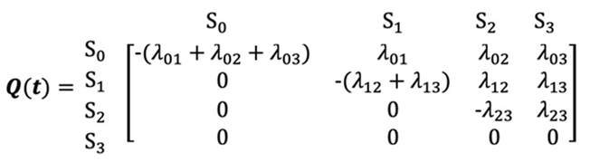
The survival risks, or state occupation probabilities, are the probability of an individual being in each state at a given time point. These probabilities can be represented as a vector, in which each value denotes the probability of being in a state, and the elements of the vector sum to 1. Suppose all participants start from S0 state, the survival risks can be estimated nonparametrically using the Aalen-Johansen (A-J) estimator.[29]
Where is the transition rate matrix, I is the identity matrix, and is the survival risk vector.
Appendix 3 illustrates the estimation of the survival risks for a four-state process using the A-J estimator. The estimated survival risk across disease states are equivalent to estimating survival risks using the Kaplan-Meier estimator by allowing individuals to transition from the starting state to multiple endpoints and by allowing individuals to transition dynamically in and out intermediate states. It is therefore evident that the Aalen-Johansen estimator is a natural extension of the Kaplan-Meier estimator to multi-state settings (Table 3).
4.3. Markov Cox Model
Under the Markov assumption (Assumption 2), the Cox model models hazards between state transition.[30] Based on this assumption, if we divide a person’s follow-up time according to the disease states they occupy, the resulting separated follow-up intervals are independent. Assumption 2 is essentially an extension of Assumption 1, in which an individual’s person-time observations are independent of one another, with the conditioning variables including not only covariates but also disease states.
Assumption 2 (Markov assumption).
By conditioning on the present state, the future transition rates are independent of the past history.
Under Assumption 2, follow-up time can be divided into data subsets according to the disease state occupied. Figure 5 shows how the follow-up data is divided into state-specific subsets. Subset 1 (blue) begins in S0 and ends in S0, S1, S2, or S3. Subset 2 (red) begins in S1 and ends in S1, S2, or S3. Subset 3 (green) begins in S2 and ends in S2 or S3. Within each subset, Cox models are applied to model hazards of transition between states. Specifically, three Cox models are fitted to data subset 1, two Cox models to subset 2, and one Cox model to subset 3.
where is the hazard of transition from state r to state s, is the baseline hazard of transition from state r to state s, and is the coefficient of X with the log hazard of developing state from state r.
For survival risk estimation using the Markov Cox model, the cumulative transition hazard is estimated from the corresponding Cox model using the Breslow estimator (or the Nelson-Aalen estimator). Rather than applying the cumulative transition hazard to estimate survival risks like the Cox model or the cause-specific Cox model, the Markov Cox model estimates transition hazards at each time point as the change in cumulative transition hazard at a time point.[31,32] These estimated transition hazards are constructed into a transition rate matrix, , and the Aalen-Johansen estimator is used to estimate the survival risks across disease states,
4.4. A Discrete-Time Split-State Framework
A discrete-time split-state framework has been proposed.[20,33,34] The motivation for this framework is that the Markov assumption is strong for chronic diseases. Take cardiovascular disease as an example, the diagnosis of one endpoint often persists across subsequent states, and there is complex interplays between metabolic risk factors in accelerating disease progression, both of which violate the Markov assumption.[35] Moreover, Markov models are memoryless and do not allow for multimorbidity, a common feature of chronic diseases.[36,37] As shown in Figure 6, the framework splits state into substates by conditioning on past states and reconstruct a process of disease substates.
This split-state approach makes a disease process both memoryless and memorable. First, split-state makes a disease process memoryless. As aforementioned, the Markov Cox models require the Markov assumption. This memoryless property restricts their ability to capture multimorbidity and the interactions among disease states in influencing disease progression. For the split-state framework, by constructing substates conditioning on past states, the substates are independent of past states and satisfy the Markov assumption even when the underlying process is non-Markovian.[20] Therefore, this framework accommodates multimorbidity and is well suitable for modeling transition of chronic diseases. Second, split-state makes a disease process memorable. As the substates are constructed by conditioning on past states, they inform past history, or temporality of multimorbidity development.[34] Thus, the framework can synthesize survival risks across all substates over time into summary measures: disease trajectories for prediction use, and multimorbidity-adjusted life year (MALY) for comparing treatment strategies.33
For model estimation, it is a natural extension of pooled logistic regression in single endpoint to a multi-state setting. Within each data subset shown in Figure 5, it considers the transition from one to multiple endpoints as competing risks. It cuts time into small intervals and changes the data structure from wide to long format and fits cause-specific Cox models (or multinormal pooled logistic regression) to estimate survival risks within each interval to approximate hazard (see the special case in Section 1.3 for using Cox models to estimate survival risks in a small time interval to approximate hazard). We include past state or their interaction with the current state as covariates into the models to allow past states to affect the transition rates of future states and relax the Markov assumption. The discrete-time transition rates are estimated from the models, and the A-J estimator is used to estimate the discrete-time survival risks of being in each substate, with 95% CI estimated using bootstrap.
This discrete-time split-state framework has three advantages.
First, the framework can be used to predict trajectories,[34] as the substates capture the temporal sequence of its development. Survival risks of being in substates, , , , , , , and , correspond to trajectories, “remaining in “, “remaining in “, “→“, “→→ “, “→“, “→→“, “→→“, and “→→→“, respectively.
Second, the discrete-time survival risks estimated from the framework allows to flexibly derive complex metrics. Specifically, the counterfactual multimorbidity-adjusted life year (MALY) under a hypothetical intervention can be estimated, where MALY is a weighted sum of survival risks in each substates over time.[33]
where is the disability weight for substate , A is a hypothetical treatment regime across disease substates, is the counterfactual survival risk at t had the person received .
A multi-state causal approach[33] has been proposed to compare effectiveness of treatment regime using MALY, where the optimal intervention is the one associated with the highest MALY.
- — is the treatment effect based on Cox models
Third, the long-format data allows flexible integration of machine learning into the framework. In addition to cause-specific Cox models (or multinominal logistic regression), machine learning methods can be applied by considering competing risks as a multi-class classification problem, where the estimated probability of each class approximates discrete-time cause-specific hazards. As mentioned in Section 3.3, this approach has been used to integrate machine learning into competing risk estimation.[26,27,28] As competing risks can be considered as a special case of a multi-state process (or a multi-state process can be viewed as a dynamic combination of multiple competing risks), it is of high interest to integrate machine learning into multi-state modeling to model discrete-time transition rates in the near future.
Summary
Taken together, this review highlights the connections among logistic regression, the Cox model, competing risk models, and multi-state modeling. It unifies the models of one single endpoint, competing risks, and multi-states in estimating hazard and survival risks. Traditional survival analyses have generated important knowledge in advancing our understanding of chronic diseases. We anticipate that multi-state modeling will play an increasingly important role in advancing the understanding of chronic disease progression and informing precision prevention and prediction of chronic diseases.
References
- Mahmood, S.S.; Levy, D.; Vasan, R.S.; Wang, T.J. The Framingham Heart Study and the epidemiology of cardiovascular disease: a historical perspective. Lancet 2014, 383(9921), 999–1008. [Google Scholar] [CrossRef] [PubMed] [PubMed Central]
- The Atherosclerosis Risk in Communities (ARIC) Study: design and objectives. The ARIC investigators. Am J Epidemiol. 1989, 129(4), 687–702. [CrossRef] [PubMed]
- Bild, D.E.; Bluemke, D.A.; Burke, G.L.; Detrano, R.; Diez Roux, A.V.; Folsom, A.R.; Greenland, P.; Jacob, D.R., Jr.; Kronmal, R.; Liu, K.; Nelson, J.C.; O’Leary, D.; Saad, M.F.; Shea, S.; Szklo, M.; Tracy, R.P. Multi-Ethnic Study of Atherosclerosis: objectives and design. Am. J. Epidemiol. 2002, 156(9), 871–81. [Google Scholar] [CrossRef] [PubMed]
- D’Agostino, R.B.; Lee, M.L.; Belanger, A.J.; Cupples, L.A.; Anderson, K.; Kannel, W.B. Relation of pooled logistic regression to time dependent Cox regression analysis: the Framingham Heart Study. Stat. Med.;PubMed 1990, 9(12), 1501–15. [Google Scholar] [CrossRef] [PubMed]
- Breslow, N.E.; Day, N.E. Statistical methods in cancer research. In The analysis of case-control studies; International Agency for Research on Cancer, 1980; Vol. 1. [Google Scholar]
- Prentice, R.L.; Breslow, N.E. Retrospective studies and failure time models. Biometrics 1978, 34(1), 57–67. [Google Scholar] [PubMed]
- Breslow, N.E.; Day, N.E.; Halvorsen, K.T.; Prentice, R.L.; Sabai, C. Estimation of multiple relative risk functions in matched case-control studies. Am. J. Epidemiol.;PubMed 1978, 108(4), 299–307. [Google Scholar] [CrossRef] [PubMed]
- Kaplan, E.L.; Meier, P. Nonparametric estimation from incomplete observations. J. Am. Stat. Assoc. 1958, 53(282), 457–81. [Google Scholar] [CrossRef]
- Nelson, W. Hazard plotting for incomplete failure data. J. Qual. Technol. 1969, 1(1), 27–52. [Google Scholar] [CrossRef]
- Aalen, O.O. Nonparametric inference for a family of counting processes. Ann. Stat. 1978, 6(4), 701–26. [Google Scholar] [CrossRef]
- Cox, D.R. Regression Models and Life-Tables. J. R. Stat. Soc. Ser. B (Methodological) 1972, 34(2), 187–220. [Google Scholar] [CrossRef]
- Kalbfleisch, J.D.; Prentice, R.L. Marginal likelihoods based on Cox’s regression and life model. Biometrika 1973, 60(2), 267–78. [Google Scholar] [CrossRef]
- Breslow, N.E. Discussion of the paper by Dr. Cox. J. R. Stat. Soc. Ser. B (Methodological) 1972, 34(2), 216–7. [Google Scholar] [CrossRef]
- Young, J.G.; Cain, L.E.; Robins, J.M.; O’Reilly, E.J.; Hernan, M.A. Comparative effectiveness of dynamic treatment regimes: an application of the parametric g-formula. Stat. Biosci. 2011, 3(1), 119–43. [Google Scholar] [CrossRef] [PubMed] [PubMed Central]
- Robins, J.M. Marginal structural models. Proc. Sect. Bayesian Stat. Sci. 1999, 1–10. [Google Scholar]
- Hernan, M.A.; Brumback, B.; Robins, J.M. Marginal structural models to estimate the causal effect of zidovudine on the survival of HIV-positive men. Epidemiology 2000, 11(5), 561–70. [Google Scholar] [CrossRef] [PubMed]
- Hernán, M.A.; Robins, J.M. Causal Inference: What If; Chapman & Hall/CRC: Boca Raton, 2020. [Google Scholar]
- Kvamme, H.; Borgan, O. Continuous and discrete-time survival prediction with neural networks Epub 20211007. Lifetime Data Anal. 2021, 27(4), 710–36. [Google Scholar] [CrossRef] [PubMed] [PubMed Central]
- Schmid, M.; Welchowski, T.; Wright, M.N. Discrete-time survival forests with Hellinger distance decision trees. Data Min. Knowl. Disc 2020, 34, 812–32. [Google Scholar] [CrossRef]
- Ding, M.; Chen, H.; L., F.C. A discrete-time split-state framework for multi-state modeling with application to describing the course of heart disease. BMC Med. Res. Methodol. 2025, 25–54. [Google Scholar] [CrossRef] [PubMed]
- Lin, D.Y. Non-parametric inference for cumulative incidence functions in competing risks studies. Stat. Med. 1997, 16(8), 901–10. [Google Scholar] [CrossRef] [PubMed]
- Prentice, R.L.; Kalbfleisch, J.D.; Peterson, A.V., Jr.; Flournoy, N.; Farewell, V.T.; Breslow, N.E. The Analysis of Failure Times in the Presence of Competing Risks. Biometrics 1978, 34, 541–54. [Google Scholar] [CrossRef] [PubMed]
- Fine, J.P.; Gray, R.J. A proportional hazards model for the subdistribution of a competing risk. J. Am. Stat. Assoc. 1999, 94(446), 496–509. [Google Scholar] [CrossRef] [PubMed]
- Robins, J. A New Approach to Causal Inference in Mortality Studies with a Sustained Exposure Period—–Application to Control of the Healthy Worker Survivor Effect. Math. Model. 1986, 7, 1393–512. [Google Scholar] [CrossRef]
- Lee, M.; Feuer, E.J.; Fine, J.P. On the analysis of discrete time competing risks data. Biometrics 2018, 74(4), 1468–81. [Google Scholar] [CrossRef] [PubMed]
- Sparapani, R.; Logan, B.R.; McCulloch, R.E.; Laud, P.W. Nonparametric competing risks analysis using Bayesian Additive Regression Trees Epub 20190107. Stat. Methods Med. Res. 2020, 29(1), 57–77. [Google Scholar] [CrossRef] [PubMed] [PubMed Central]
- Janitza, S.; Tutz, G.; Boulesteix, A.L. Random forest for ordinal responses: Prediction and variable selection. Comput. Stat. Data Anal. 2016, 96, 57–73. [Google Scholar] [CrossRef]
- Schmid, M.; Berger, M. Competing risks analysis for discrete time-to-event data. WIREs Comput Stat. 2021, 13, e1529. [Google Scholar] [CrossRef]
- Aalen, O.O.; Johansen, S. An empirical transition matrix for non-homogeneous Markov chains based on censored observations. Scand. J. Stat. 1978, 5(3), 141–50. [Google Scholar]
- Andersen, P.K.; Keiding, N. Multi-state models for event history analysis. Stat. Methods Med. Res. 2002, 11(2), 91–115. [Google Scholar] [CrossRef] [PubMed]
- Putter, H.; Fiocco, M.; Geskus, R.B. Tutorial in biostatistics: competing risks and multi-state models. Stat Med. 2007, 26(11), 2389–430. [Google Scholar] [CrossRef] [PubMed]
- de Wreede, L.C.; Fiocco, M.; Putter, H. The mstate package for estimation and prediction in non- and semi-parametric multi-state and competing risks models Epub 20100315. Comput Methods Programs Biomed. 2010, 99(3), 261–74. [Google Scholar] [CrossRef] [PubMed]
- Ding, M. Estimating the effects of treatment regimes over the course of chronic disease: A multi-state causal framework with baseline confounding. Stat. Methods Med. Res. 2026. [Google Scholar] [CrossRef] [PubMed]
- Ding, M.; Lin, F.C.; Meyer, M.L. Summary Measures Derived from a Multi-state Modeling Framework to Characterize the Course of Heart Disease. BMC Med. Res. Methodol. 2026. [Google Scholar] [CrossRef] [PubMed] [PubMed Central]
- Ndumele, C.E.; Rangaswami, J.; Chow, S.L.; Neeland, I.J.; Tuttle, K.R.; Khan, S.S.; Coresh, J.; Mathew, R.O.; Baker-Smith, C.M.; Carnethon, M.R.; Despres, J.P.; Ho, J.E.; Joseph, J.J.; Kernan, W.N.; Khera, A.; Kosiborod, M.N.; Lekavich, C.L.; Lewis, E.F.; Lo, K.B.; Ozkan, B.; Palaniappan, L.P.; Patel, S.S.; Pencina, M.J.; Powell-Wiley, T.M.; Sperling, L.S.; Virani, S.S.; Wright, J.T.; Rajgopal Singh, R.; Elkind, M.S.V.; American Heart, A. Cardiovascular-Kidney-Metabolic Health: A Presidential Advisory From the American Heart Association Epub 20231009. Circulation 2023, 148(20), 1606–35. [Google Scholar] [CrossRef] [PubMed]
- Drozd, M.; Relton, S.D.; Walker, A.M.N.; Slater, T.A.; Gierula, J.; Paton, M.F.; Lowry, J.; Straw, S.; Koshy, A.; McGinlay, M.; Simms, A.D.; Gatenby, V.K.; Sapsford, R.J.; Witte, K.K.; Kearney, M.T.; Cubbon, R.M. Association of heart failure and its comorbidities with loss of life expectancy Epub 20201105. Heart. 2021, 107(17), 1417–21. [Google Scholar] [CrossRef] [PubMed] [PubMed Central]
- Khan, M.S.; Samman Tahhan, A.; Vaduganathan, M.; Greene, S.J.; Alrohaibani, A.; Anker, S.D.; Vardeny, O.; Fonarow, G.C.; Butler, J. Trends in prevalence of comorbidities in heart failure clinical trials. Eur. J. Heart Fail. 2020, 22(6), 1032–42. [Google Scholar] [CrossRef] [PubMed] [PubMed Central]
Figure 1.
The connections among pooled logistic regression, conditional logistic regression, and the Cox model. Figure 1a shows the data for each person, where indicates an event. Figure 1b divides follow-up time into equal small intervals, which are independent of each other. Figure 1c changes the data structure from wide to long format and fits a pooled logistic regression model. Figure 1d creates a risk set at each event time, and these risk sets are independent of each other. For a matched case-control study, controls can be randomly sampled from each risk set, and a conditional logistic regression model can be fitted. In a Cox model, these risk sets are used to construct the partial likelihood for parameter estimation. The conditional likelihood used in conditional logistic regression is equivalent to the partial likelihood used in the Cox model.
Figure 1.
The connections among pooled logistic regression, conditional logistic regression, and the Cox model. Figure 1a shows the data for each person, where indicates an event. Figure 1b divides follow-up time into equal small intervals, which are independent of each other. Figure 1c changes the data structure from wide to long format and fits a pooled logistic regression model. Figure 1d creates a risk set at each event time, and these risk sets are independent of each other. For a matched case-control study, controls can be randomly sampled from each risk set, and a conditional logistic regression model can be fitted. In a Cox model, these risk sets are used to construct the partial likelihood for parameter estimation. The conditional likelihood used in conditional logistic regression is equivalent to the partial likelihood used in the Cox model.
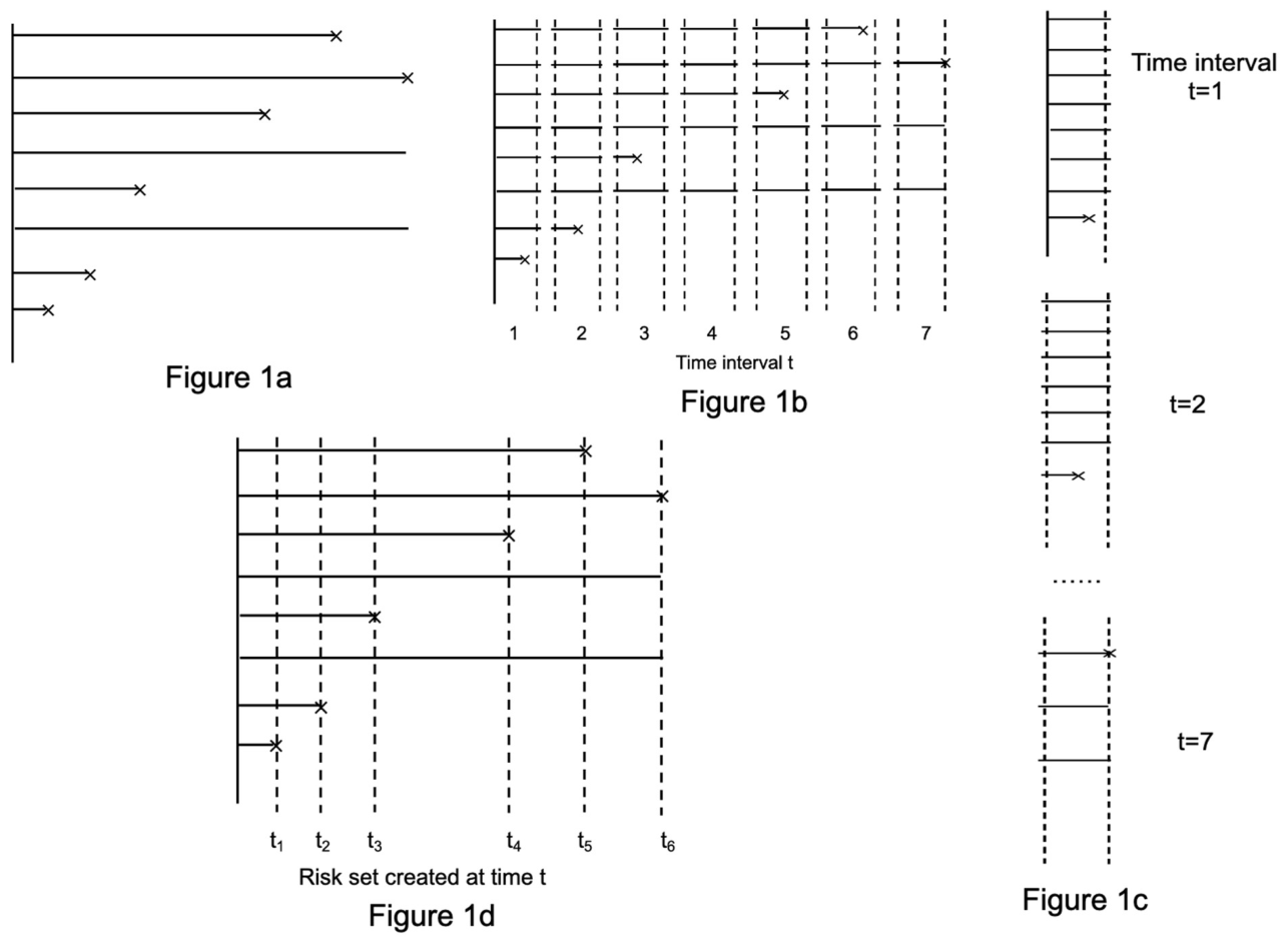
Figure 2.
An illustration of estimating the discrete-time hazard using the Cox model.[20] Figure 2a shows the long-format data structure, where a Cox model is fitted and the time interval t is modeled as a counting variable (t=1, 2, 3, …). The dashed lines (--) show how the estimated hazard changes with time within each interval. As expected, the hazards are proportional across t. The solid lines (—) show that the hazard within each interval can be approximated by the survival risk at a time point within the interval. Figure 2b shows the true hazard (--), the hazard within each time interval estimated using the Cox model (--), and the hazard approximated by survival risk (—).
Figure 2.
An illustration of estimating the discrete-time hazard using the Cox model.[20] Figure 2a shows the long-format data structure, where a Cox model is fitted and the time interval t is modeled as a counting variable (t=1, 2, 3, …). The dashed lines (--) show how the estimated hazard changes with time within each interval. As expected, the hazards are proportional across t. The solid lines (—) show that the hazard within each interval can be approximated by the survival risk at a time point within the interval. Figure 2b shows the true hazard (--), the hazard within each time interval estimated using the Cox model (--), and the hazard approximated by survival risk (—).
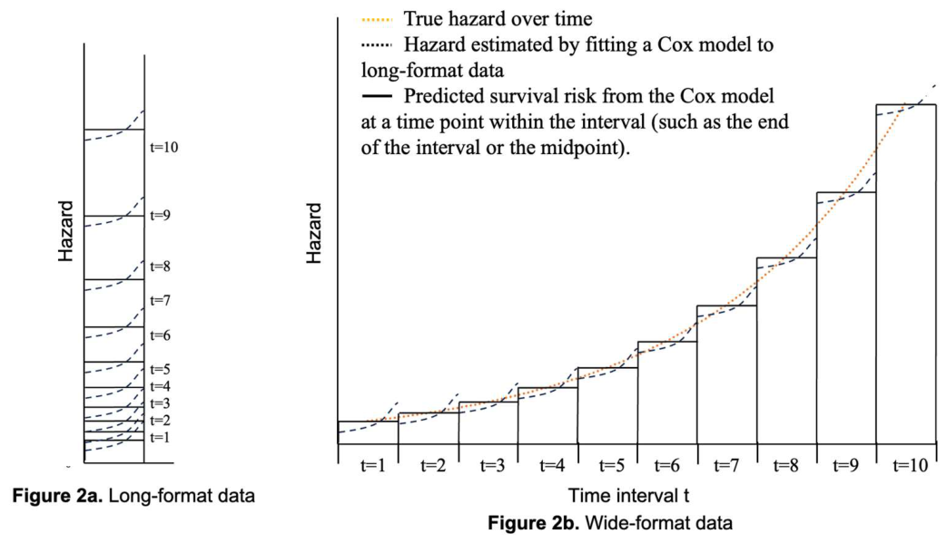
Figure 3.
Conceptual Comparison of Competing Risks Analysis Using Separate Cox Models for Each Cause, the Cause-Specific Cox Model, and the Fine–Gray Model.
Figure 3.
Conceptual Comparison of Competing Risks Analysis Using Separate Cox Models for Each Cause, the Cause-Specific Cox Model, and the Fine–Gray Model.
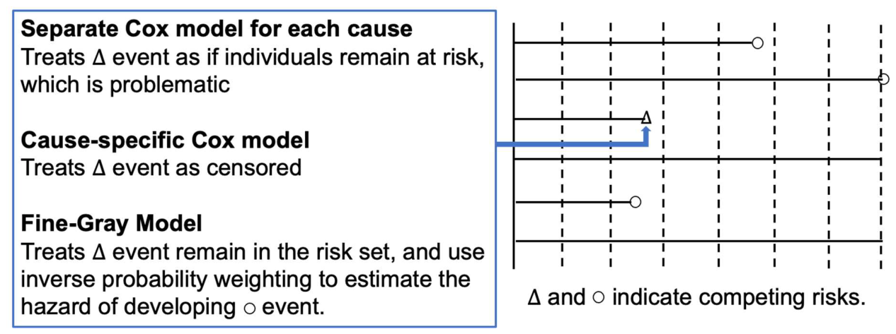
Figure 4.
Afour-state transition process.
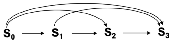
Figure 5.
Data Structure for Multi-State Modeling.
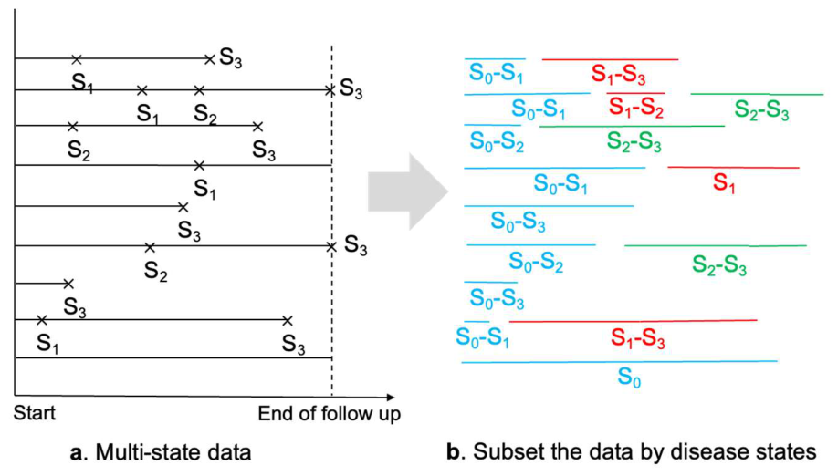
Figure 6.
A discrete-time split-state framework for multi-state modeling.
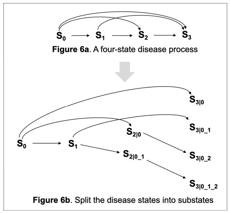

Table 1.
Comparison of continuous-time and discrete-time approaches for modeling hazard and estimating survival risks in single endpoint, competing risks, and multi-state settings.
Table 1.
Comparison of continuous-time and discrete-time approaches for modeling hazard and estimating survival risks in single endpoint, competing risks, and multi-state settings.
| Single endpoint | ||
| Model | Cox model | Pooled logistic regression |
| Risk sets | Risk sets are created when an event occurs (Figure 1d) | Risk sets are created with equal time intervals (Figure 1b) |
| Modeling hazard | Continuous time |
Discrete time, incidence rate within each interval approximates hazard |
| Likelihood | Partial likelihood, baseline hazard cancels out | Full likelihood, baseline hazard modeled by including functions of time interval |
| Survival risk estimation | Continuous time, Breslow estimator |
Discrete time, Kaplan-Meier estimator |
|
R packages for survival risk estimation |
survival::coxph() to fit the Cox model, and predict() to estimate survival risk | survival::survSplit() to create long-format data, followed by glm(family = binomial) for pooled logistic regression; interval-specific hazard predicted using predict(), then combined using Kaplan-Meier estimator to estimate survival risks |
| Computational burden | Efficient | More computational by using bootstrap to estimate 95% confidence interval |
| Accuracy | More accurate by modeling continuous-time hazard | Incidence rate approximates hazard |
|
Advantages |
|
|
| Competing risks | ||
| Model | Cause-specific Cox models | Multinomial logistic regression |
| Risk sets | Risk sets are created when competing events occur | Risk sets are created with equal time intervals |
| Modeling hazards | Continuous time | Discrete time |
| Likelihood | Cox partial likelihood for each cause | Full likelihood for each cause |
| Survival risk estimation | Continuous time, Cumulative incidence function (CIF) |
Discrete time, CIF function |
|
R packages for survival risk estimation |
riskRegression::CSC() to fit Cox models, and predict() to estimate survival risks using CIF. |
survival::survSplit() to create long-format data, followed by nnet::multinom() for multinominal logistic regression; interval-specific hazards predicted using predict(), then combined using CIF to estimate survival risks |
| Computational burden | Efficient | More computational |
| Accuracy | More accurate | Incidence rates approximate hazards |
| Advantages | Efficient, Accurate |
The discrete-time hazards are flexible for estimating complex statistics such as causal inference methods; easy to integrate machine learning methods into competing risk analysis |
| A multi-state process | ||
| Model | Multi-state Cox model | A discrete-time split-state framework |
| Risk sets | Subset longitudinal data by disease states. Then create risk sets same as the cause-specific Cox model. | Subset longitudinal data by disease states. Then create risk sets same as the multinomial logistic regression. |
| Modeling hazards | Continuous time | Discrete time |
| Likelihood | Within each data subset, Cox partial likelihood for each cause | Within each data subset, full likelihood for each cause |
| Survival risk estimation | Continuous time, Aalen-Johansen (A-J) estimator |
Discrete time, A-J estimator |
|
R packages for survival risk estimation |
mstate to fit transition-specific Cox models, and probtrans() to estimate survival risks | survival::survSplit() to create long-format data, followed by nnet::multinom() for multinominal logistic regression; interval-specific hazards predicted using predict(), then combined to estimate survival risks using A-J estimator |
| Computational burden | Efficient | More computational |
| Accuracy | More accurate | Incidence rates approximate hazard |
| Advantages |
Efficient, Accurate |
The discrete-time hazards are flexible to for estimating complex statistics such as causal inference methods; easy to integrate machine learning methods into multi-state analysis |
Table 2.
An example illustrating why the cumulative incidence function (CIF), rather than the Kaplan-Meier (K-M) estimator, should be used to estimate the cumulative incidence of competing events.
Table 2.
An example illustrating why the cumulative incidence function (CIF), rather than the Kaplan-Meier (K-M) estimator, should be used to estimate the cumulative incidence of competing events.
| Cause | t1 | t2 | t3 | |
| Hazard | 1 | 0.5 | 0.3 | 0.4 |
| Hazard | 2 | 0.4 | 0.6 | 0.5 |
| Cumulative incidence estimated using K-M estimator for each cause | ||||
| Incidence | 1 | 0.5 | 0.15 | 0.14 |
| Cumulative incidence | 1 | 0.5 | 0.65 | 0.79 |
| Incidence | 2 | 0.4 | 0.24 | 0.18 |
| Cumulative incidence | 2 | 0.4 | 0.64 | 0.82 |
| Cumulative incidence | 1 or 2 | 0.9 | 1.29 | 1.61 |
| Survival risk | 0 | 0.1 | -0.29 | -0.61 |
| Cumulative incidence estimated using CIF | ||||
| Incidence | 1 | 0.5 | 0.03 | 0.004 |
| Cumulative incidence | 1 | 0.5 | 0.53 | 0.534 |
| Incidence | 2 | 0.4 | 0.06 | 0.005 |
| Cumulative incidence | 2 | 0.4 | 0.46 | 0.465 |
| Cumulative incidence | 1 or 2 | 0.9 | 0.99 | 0.999 |
| Survival risk | 0 | 0.1 | 0.01 | 0.001 |
We used discrete-time hazard as an example.
Table 3.
Nonparametric estimation of survival risks based on hazards for a single endpoint, competing risks, and a multi-state process.
Table 3.
Nonparametric estimation of survival risks based on hazards for a single endpoint, competing risks, and a multi-state process.
|
Single endpoint |
Competing risks |
A multi-state process (a four-state transition as an example) |
|
|
Hazard |
|
|
|
| Survival risk |
|
||
| Estimation method | Kaplan-Meier estimator | Cumulative incidence function (CIF) | Aalen-Johansen (A-J) estimator |
|
Note |
is the number of cases at time t, and is the number of participants in the risk set at time t. | is hazard due to cause is the number of cases due to cause at time t, is the number of participants in the risk set, and is the survival risk at time t. | is the transition rate matrix, where we assume constant hazard of transition. is an identity matrix. |
We used discrete-time hazards and survival risks as an example.
Disclaimer/Publisher’s Note: The statements, opinions and data contained in all publications are solely those of the individual author(s) and contributor(s) and not of MDPI and/or the editor(s). MDPI and/or the editor(s) disclaim responsibility for any injury to people or property resulting from any ideas, methods, instructions or products referred to in the content. |
© 2026 by the authors. Licensee MDPI, Basel, Switzerland. This article is an open access article distributed under the terms and conditions of the Creative Commons Attribution (CC BY) license (http://creativecommons.org/licenses/by/4.0/).
Copyright: This open access article is published under a Creative Commons CC BY 4.0 license, which permit the free download, distribution, and reuse, provided that the author and preprint are cited in any reuse.