

Submitted:
14 August 2026
Posted:
17 August 2026
You are already at the latest version
Abstract
Event-based vision sensors (EVS) offer an innovative approach to optical sensing by responding solely to changes in photon flux with asynchronous pixels. This enables high-speed imaging with minimal data throughput and a large dynamical range >120dB. Despite their growing use in edge detection and the observation of Earth science phenomena such as lightning and transient luminous events (TLEs), optimizing EVS performance specifically for high-speed obervations on microsecond timescales, where the photon flux is key, remains challenging. This is due to the unitless, non-intuitive nature of their bias settings, which drives the working principles of the sensor. In this study, we perform a comprehensive calibration of an event-based camera, focusing on three critical parameters: contrast thresholds, refractory period, and corner frequency of the inherent low-pass filter. Using a pre-calibrated LED source and newly developed event generation code, we establish physical relationships between these raw digital bias settings and the camera's response characteristics. Our results show tunable ranges of 5%–190% for contrast thresholds, 12–480 \(\mu\)s for refractory periods, and 1–11 kHz for corner frequencies. These calibrations provide the fundamental camera characteristics for accurate optical signal reconstruction and improved detection of fast transient phenomena. The approach is demonstrated on a Prophesee EVK4; however, the proposed calibration method can be applied to any EVS camera that employs similar hardware components and bias settings, providing a necessary framework for the quantitative use of EVS cameras in atmospheric remote sensing.
Keywords:
event based/neuromorphic cameras
; remote high-speed observations
; atmospheric electricity
1. Introduction
Over the past 15 years, the development and use of event-based vision sensors (EVSs) have gained significant attention for remote sensing applications as a novel neuromorphic sensor that mimics the principles of retinal neurons. EVSs relies on asynchronous pixels using a special analog circuitry that acts as a temporal contrast sensor, transmitting data only in response to changes in the photon flux hitting the pixel [1,2].
Unlike traditional cameras, no frames or constant sampling rate is used. In turn, the individual pixel acts dynamically and individually based on its own received optical signal. When the variation in the logarithm of the photon flux exceeds a certain threshold value, the pixel will generate an event that is defined by four parameters : the pixel coordinates (x, y), the event polarity: 1 for increased brightness (on event) or 0 for decreased brightness (off event) and a timestamp.
The performance of the sensor can be tuned by varying the so-called bias settings to control the camera behavior in different ways. In total, four tunable raw digital bias settings are accessible by the user [3], including those for the corner frequency of the low/high pass filter, a refractory period corresponding to a dead time for each pixel after an event, and the on / off thresholds related to the generation of on / off events [4]. These properties make the EVS capable of working at a high temporal resolution of 1-10 and a large dynamic range of , with a low data rate and low power consumption [2,5]. These capabilities, furthermore, makes the EVS perfect for remote sensing purposes as their operational requirements are low, compared with conventional frame-based high-speed cameras.
Previous studies on EVS have focused on using its high dynamic range and low data rate for applications such as autonomous vehicles, drones, motion detection, satellite tracking and monitoring [6,7,8,9,10]. One can also note that the sparse, asynchronous nature of EVS data makes it well-suited to machine learning algorithms. Recently, additional efforts have been made to study natural phenomena in Earth sciences, including auroras, meteors, lightning, and Transient Luminous Events (TLEs) in the upper regions of the atmosphere above thunderstorms [11,12,13]. These studies highlight the potential of EVS for high-speed optical observations from space, particularly for future satellite lightning mapping. Its high temporal resolution, wide dynamic range, and low data rate make it a promising technology for next-generation lightning imagers. However, it is crucial to understand the exact working principles of the camera and to fine-tune the individual bias settings. This allows for optimizing the camera settings for any given scenario.
Furthermore, standard calibration methods for frame-based cameras are not sufficient when calibrating an event camera. For frame-based cameras, this is usually done with a static source with known intensity. As the event camera requires changes in the photon flux, it is necessary to have a tunable calibration source where the light level is known both at the lowest and largest luminosities.
Other calibration work has focused mainly on optimizing quality metrics for the generated event streams [14]. However, our main interest is high-speed observations of electrical discharges in the atmosphere, such as lightning and TLEs, and related physical processes. They occur extremely fast on millisecond time scales, with some sub-processes even reaching microsecond time scales [15]. Thus, we focus on assessing the temporal resolution of the EVS and calibrating the most relevant bias settings, particularly the low-pass-filter corner frequency and the refractory period associated with the pixel dead time.
The paper is based on experimental data from a blinking pre-calibrated LED diode measured with a Prophesee EVK4 camera 1. The EVK4 camera is based on the Sony IMX636 sensor co-developed with Prophesee 2. The sensor consists of pixels of size 4.86 µm × 4.86 µm, offering a dynamic range 120 dB and a maximum event rate (Giga-events per second) with low power consumption. Additionally, it also offers the possibility of choosing a region of interest (ROI), consequently making the other pixels inactive.
2. Bias Setting Parameters of Event-Based Camera
Event camera data consist of an event stream of tuples, where indicates the position of the pixel that generated the event, p represents the polarity, with “1" for an on event and “0" for an off event, and t is the timestamp of the event in s. The sensor offers a range of bias settings that alter performance. The four bias settings of interest for high-speed observations are the on/off threshold, the corner frequency affecting the low-pass filter, and the refractory period that introduces a dead time for each individual pixel. An overview of the bias settings for the EVK4 camera with their individual range and effects are shown in Table 1.
A simulated example showing the effects of different bias settings on a single pixel is shown in Figure 1. We applied two different low-pass filter settings with corner frequency () and to show the effect of the low-pass filter. The thresholding for on/off event generation is checked on the filtered signals, thus a threshold of 5% is not directly translated to a 5% change in photon flux but on the low-pass filtered signal corresponding to it. The effect of refractory period is also shown in the figure; here the refractory period is set to 200 µs. During this dead-time the generation of event is ignored, but the pixel still samples the analog signal internally such that the reading at the end of the refractory period defines the new comparative light level. This defines the new reference light level, which is also shown in the figure.
Therefore, accurate estimation of the variation of photon flux from event stream data requires not only knowledge of the contrast threshold settings, but also the corner frequency and the refractory period. These aspects will be further discussed in the following sections.
3. Calibration Parameters for Event-Based Cameras
3.1. Threshold
EVS cameras have independent and asynchronous pixels that respond to changes in the logarithm of the brightness signal [16]. An “on" event is triggered when the magnitude of the logarithm brightness level has increased by more than an “on" threshold of for an individual pixel at a time . For the sake of simplicity, we assume very slow changes in light levels, such that we can ignore the effects of the refractory period and the low-pass filter. In this case, the event generation follows the increasing photocurrent I reaching :
where L is the log photocurrent . Conversely, an “off" event corresponds to a photocurrent decrease by reaching a “off" threshold of . The threshold of EVK4 camera is defined with three bias settings: bias_diff, bias_diff_on and bias_diff_off. In general, it follows,
where is a default bias current set with the setting bias_diff, which is advised to be kept constant. Both and are bias currents, considered as variables, and are set with the bias settings bias_diff_on and bias_diff_off, respectively. is a factor that depends on the electrical characteristics of the sensor.
In our calibration, we aim to determine how bias setting changes in bias_diff_on and bias_diff_off affect the percentage change in the light level. We first simulate a “star field" with stars of known magnitudes for the EVK4 camera by varying the input current of a Spacecraft Optical Ground Support Equipment (SOGSE provided by Terma A/S) based on a calibrated (amber) LED [17]. We use a 1 Hz triangular wave such the influence of the refractory period and the low-pass filter is negligible. Then we measure the ratio of maximum and minimum log photocurrent ( and ) of the triangular wave based on a calibrated HAMAMATSU photomultiplier 3.
The percentage change in the detected light level can be estimated based on the effect of a single threshold change [18,19]:
where is the maximum number of the generated on/off events in a single pixel measured by the EVK4 camera. is the relative change of the light intensity to create an event. As our main goal is observing transient phenomena such as lightning, we are also interested in balanced bias settings that produce a similar number of on and off events as a response to ensure that the measured light decreases corresponds to the light increases.
3.2. Refractory Period
The refractory period of the camera, also known as the dead time of an individual pixel, is an amount of time after the production of an event where the pixel is inactive. It is controlled by the bias setting of bias_refr. In general, the time between two events on a given pixel is , where is the time it takes for the optical signal to pass a threshold level above the reference value at time , and is the refractory period after the latest generated event. The refractory period can be estimated by changing the signal fast enough for , from which an upper limit of the dead time can be estimated by finding the smallest observed in the distribution of received events.
This is done by sending 100 kHz sine waves to the LED with a function generator, lowering the thresholds to a minimum level [], ensuring a negligible such that measuring the minimum value of corresponds to measuring the refractory period for each refractory period bias setting.
3.3. Low-Pass Filter
The generation of events is affected by the low-pass filtering. This effect is controlled by the bandwidth bias setting of bias_fo. It is often used to remove flickering and noise from the scene, but we are interested in its effect on high-speed observations and investigate how changing bias_fo affects the corner frequency of the low-pass filter [20].
For this purpose, we use an event generation model based on a first-order infinite impulse response (IIR) low-pass filter with a constant corner frequency [20] by taking both the on/off thresholds and the refractory period into account. The filtered signal received at the single-pixel level will follow,
where is the time constant, defined by the corner frequency as , n being the event registrered and being the time difference from the
n-1 to the event. L being the original log (photocurrent) from Equation 1 and being the filtered signal. The corner frequency can be determined by generating sine waves for the LED source using a function generator with varying input frequencies. By applying different bias_fo and changing the input frequency of the LED signal, the number of generated on/off events for a defined region of pixels is recorded to evaluate the corner frequency which follows Equation (6).
In order to determine , we simulate the pixel response to LED sine wave signals using the same frequencies as those used in the measurements, taking into account both the refractory period used for the measurements and the estimated pixel threshold mismatch. This enables evaluating the simulated corner frequency that minimizes the difference between the simulated and measured results for different bias_fo settings.
4. Results
The calibration of the EVS requires three distinct measurements, which can allow for reconstruction of the optical signal for high-speed observation. This includes a threshold estimation, an estimation of the refractory period, and a measurement of the corner frequency associated with the low pass filtering.
4.1. Threshold Calibration
The threshold was estimated using a pre-calibrated SOGSE provided by TERMA. This equipment simulates a star field of which the intensity is slowly altered by changing the voltage level on the LED with a triangular wave between 3 V and 5 V at a frequency of 1 Hz.
Assuming, the illumination of "star" fed with a voltage of 3 V and 5 V, corresponds to a photon-current of and respectively, Equations (4) and (5) can be used to find the threshold or when the peak number of on or off events ( or ) is measured.
We also measure the thresholds that produce a similar number of on and off events, we adjust bias_diff_on and bias_diff_off accordingly at a refractory period of 50 µs. The results of this matching process are shown in Figure 2(A). Figure 2(B) presents the calibrated curve of the on and off thresholds as a function of the bias_diff_on setting. The inset illustrates an example fit for the threshold settings used to determine the peak event value.
4.2. Refractory Period Calibration
As described in the preceding section, we measured the refractory period by finding the shortest time between consecutive events illuminated by a star field modulated with a 100 kHz sine-wave voltage, and the contrast thresholds are set to based on the measurement shown in Figure 2(B). The results are shown in Figure 3(A) which gives the refractory period as a function of the bias setting. Results obtained from the tabulated values in the Prophesee API function are also shown in the figure for comparison 4. Both curves show similar behavior, with a logarithmic scaling of the refractory period vs. the setting. From the measurement we are however able to reach slightly lower refractory periods at the largest bias settings. This refractory period can be tuned approximately from 12–480 µs by applying different settings. Figure 3(B) Show two examples of refractory period measurements. The top panel shows the fastest setting where 12 µs. The bottom panel shows the slowest possible setting where 480 µs.
4.3. Corner Frequency Calibration
The calibration of the corner frequency aims to determine the value of in Equation (6), which is associated with the setting . The frequency of the sine-wave modulation applied to the LED source was varied over a wide range (1 Hz, 5 Hz, 10 Hz, 50 Hz, 100 Hz, 500 Hz, 1 kHz, 2 kHz, 3 kHz, 4 kHz, 5 kHz, 6 kHz, 7 kHz, 8 kHz, 9 kHz, 10 kHz, 20 kHz, 30 kHz, 40 kHz, and 50 kHz) for nine different settings of . For these measurements, the on/off thresholds were set using Figure 2, such that . As the period of the fastest signals was on the order of 100 µs, the refractory period was set to the maximum bias setting() to avoid significant influence from this bias setting. For a region of pixels, the total number of on and off events registered per cycle is estimated and shown in Figure 4.
We can see from the figure that the high-frequency components have been filtered out by the low-pass filter of the event camera. Notably, for the measurement curves have a similar feature just below 10 kHz where the measurements overlap. This effect is due to the limitation imposed by the refractory period.
To estimate the corner frequency , we simulate the generation of events using an event generation code based on Equations (1)–(6), We simulated the event response at the single-pixel level to a sine signal. Figure 5 shows a simulation of a single ideal pixel, with a set threshold and no refractory period for different simulated corner frequencies. The amplitude of the simulated sine wave is set such that the simulated event count/cycle matches the measured values at 100 Hz. The simulations of this ideal pixel is compared with the measurements for a low-pass filter bias setting (black curve). The result shows that the simulations do not capture the measurements. To explain and correct this discrepancy, we introduce the refractory period and the effect of threshold mismatch in the model. The latest is modeled by simulating the average pixel response over 500 pixels with slightly different thresholds. To do so, each pixel threshold is chosen from a Gaussian distribution of the parameters found by matching the measured event distribution and the simulated one, as seen in Figure 6(A) and Figure 6(B). The Gaussian distribution that matches the measured event distribution has a mean of and a . We now resimulate the average pixel response of 500 pixels, with a refractory period of 12 µs and the previously found threshold mismatch. The results are presented in Figure 7(A) and Figure 7(B). The comparison is made for on and off events at using different corner frequencies. It is noted that the corner frequency of 9000 Hz best matches the measurement when using for both on and off events. Figure 7(C) and Figure 7(D) show the residuals by calculating the difference between the measured and simulated values. As both On and Off measurements rely on the same setting, we chose the best simulated value as the corner frequency that match both measurements. However, matching the On events the best are of greatest importance for high-speed imaging of lightning processes, which is our main interest. Thus, for the results shown in the figure, we consider to be best across the entire frequency range. Furthermore, the residuals show an acceptable agreement over the entire frequency range, with fluctuations around a perfect match.
This method allows to measure the corner frequency for all settings and we give the results in Figure 7(E) which gives the inferred relationship between and the corner frequency of the low-pass filter by matching the measurements with the simulations. The change in the bias_fo setting follows an S-shaped curve: it starts slowly (below the default value of 0), then rises rapidly (from 0 to 30), and finally stays nearly constant as it approaches approximately 11 kHz.
5. Discussion
5.1. Optimization
For optimizing bias settings towards high-speed operations, one can note from Figure 1, that the number of events produced on the filtered signal with a corner frequency of 1 kHz (blue) and 10 kHz (black) is the same. It appears surprising as their amplitudes are, respectively, 62 % and 95 % of the original signal, corresponding to a slew rate of and . This illustrates the effect of the refractory period, clarifying that the event generation process is occurring outside of the dead time. As the signal with the larger corner frequency is less impacted by the low pass filter, the refractory spans a larger portion of the signal, thus reducing in a larger signal loss. The amount of signal loss in this example can be estimated as 33 % and 57 %, respectively, which is correlated with the slew rate. This suggests that relatively slow low-pass and refractory period settings can still be effective for detecting fast transient signals, such as those produced by lightning and TLEs. Finally, it should be noted that the low pass filtering does not cut off high-speed signals. Thus, the EVS can observe signals that are faster than the corner frequency, however, interpretation of the result requires understanding the bias settings better. Furthermore, the amplitude of the filtered signal is strongly dependent on the corner frequency. For a strongly filtered signal, the contrast thresholds should therefore be lowered to ensure event generation.
This interpretation along with the calibrated physical parameters for the bias settings allows for a practical guide on observing different high-speed electrical phenomena. This is further shown in Table 2. Here typical time constants of different high-speed electrical phenomena, which are of interest to the authors, are shown [21,22]. This is presented along with a suggestion to the physical values of the bias settings that can be used for different observations. In most cases a low refractory period is preferred; however, it can be increased for the slower phenomena to reduce data size. For the fastest and faint phenomena it is advised to use a low refractory period, as the event generation operates after a low-pass filtering of the logarithm of the illuminance. It should be noted that these are general recommendations, and factors such as the optical system, observation distance, and the actual relative change in light intensity produced by the phenomena may vary. Therefore, the bias settings may require fine-tuning for each specific observation scenario.
Our results also give a comprehensive understanding of the low pass filtering and brightness thresholding which can serve as a basis for reconstructing the optical signal from the event-based camera by reversing the equations that govern the generation of events with the correct parameters. However, additional measurements validating the calculations are needed to support this.
Another consideration for the low-pass filtering process is that its effect depends on the illumination of the sensor. This is influenced by both the intensity of the light source and the distance to it. The corner frequency increases linearly with increasing illumination [23]. As the LED voltage is varied only between 3 V and 5 V, the effects of changes in illumination are neglected. However, it should be noted that the corner frequencies would differ when observing brighter scenes [24]. However, the effect of varying the bias_fo setting remains comparable to the reported results, although with an offset due to the linear increase in corner frequencies.
All examples listed in Table 2 are assumed to occur under low-background-intensity conditions. The experiments presented here are designed to emulate these events. At higher initial background illumination levels, a lower bias_fo setting may produce a similar or higher operational corner frequency, . Therefore, for a given bias_fo setting, the results presented in this study represent a worst-case scenario for the corner frequency.
5.2. Bandwidth Saturation
Another point we want to discuss here is the saturation that limits the maximal event rate. While the sensor does not saturate similarly to a frame based camera due to overexposure, it has a maximum feasible event rate. For the EVK4 this limitation is 1.06 Geps (Giga events pr second) across the entire sensor, or roughly . To mitigate this, an event rate controller filter in the final stage of the data processing circuit can be used to reduce the event rate by randomly discarding events that exceed the maximum allowable rate, although this comes at the cost of reduced signal quality [5]. Selecting a region of interest (ROI) may also help mitigate saturation; however, this reduces the field of view. Our work gives the tools to optimize the bias settings for signal quality and accuracy while staying below the saturation limit of the sensor.
5.3. Sensor Variation
Although the measurements were obtained using a single Prophesee EVK4 camera, they were performed across the sensor array and therefore account for pixel-to-pixel variability. Small device-to-device differences may still arise from fabrication tolerances; however, the use of factory-calibrated relative bias settings is expected to minimize their effect on the reproducibility of the results 5. The absolute bias values can be read using Prophesee software, for the camera presented here the absolute values are: bias_fo = 88, bias_diff_on = 99, bias_diff_off = 55 and bias_refr = 20. Readers are encouraged to compare these values with those of their own EVK4 cameras, as absolute factory-calibrated default values may vary slightly between devices. For other EVS cameras based on the same IMX636 sensor, such as the IDS uEye XCP-E6, SilkyEvCam HD 7 and Lucid Triton2 EVS 8, the results may also be applicable since the bias definitions are consistent with those used in the Prophesee software. Nevertheless, users are advised to reproduce a subset of the calibration points to reduce uncertainties associated with possible inter-device variations. For other types of event-based vision sensors, such as DAVIS or DVS cameras 9, the proposed calibration method can be reproduced, as they employ similar hardware components that can be controlled through corresponding bias settings.
6. Conclusions
In this work, we have characterized the EVK4 event-based camera by evaluating the ranges and physical significance of four key bias parameters that control its performance for high-speed detection. Our results show (1) the correspondence with the on/off threshold bias setting and the contrast threshold. This can be varied from 5% to 190%. (2) the correspondence between the low-pass filter bias setting and the corner frequency of the low-pass filter. This varies between 1 kHz and 11 kHz. (3) the correspondence between the dead-time bias setting and the pixel refractory period. This varies between 12 µs and 480 µs. The results of the measurements are summarized in Table 3. Note that the full operating range reported in Table 3 is not tested for the On and Off threshold bias. The range of the On threshold is limited on the lower end to restrict the range to having similar On and Off thresholds. For the high end, the threshold is limited to about 200% which is high enough for most applications and only reflects the limitation of our LED. By providing a clear mapping between the bias settings and the camera performance, we allow the reader to tune and find the best compromise when observing a given physical phenomena, especially fast processes which require high-speed observations.
Author Contributions
Conceptualization, Dongshuai Li, Oliver Chanrion, Torsten Neubert, Alejandro Luque, and Nicolas Pedersen; methodology, Dongshuai Li, Oliver Chanrion, Nicolas Pedersen and Tao Liu; software, Nicolas Pedersen and Tao Liu; validation, Dongshuai Li, Oliver Chanrion and Farhad Rachidi; formal analysis, Nicolas Pedersen; investigation, Nicolas Pedersen and Tao Liu; resources, Justo Sánchez and Francisco J. Gordillo-Vázquez; data curation, Tao Liu and Nicolas Pedersen; writing—original draft preparation, Nicolas Pedersen; writing—review and editing, Donshuai Li, Olivier Chanrion, Farhad Rachidi, Francisco J. Gordillo-Vázquez, and Alejandro Luque; visualization, Nicolas Pedersen, Dongshuai Li and Olivier Chanrion; supervision, Olivier Chanrion, Dongshuai Li, Farhad Rachidi; project administration, Dognshuai Li; funding acquisition, Dongshuai Li. All authors have read and agreed to the published version of the manuscript.
Funding
This work was supported by the Danish Council for Independent Research for a Danmarks Frie Forskningsfond (DFF) Sapere Aude Grant with Agreement 3120-00088B.
Data Availability Statement
The data that support the findings of this study are openly available at the following URL/DOI: https://doi.org/10.5281/zenodo.20374228
Conflicts of Interest
The authors declare no conflicts of interest. The funders had no role in the design of the study; in the collection, analyses, or interpretation of data; in the writing of the manuscript; or in the decision to publish the results.
Abbreviations
The following abbreviations are used in this manuscript:
| EVS | Event Based Vision Sensord |
| TLE | Transient Luminous Events |
References
- Lichtsteiner, P.; Posch, C.; Delbruck, T. A 128 128 120 dB 15 s Latency Asynchronous Temporal Contrast Vision Sensor. Proc. IEEE J. Solid-State Circuits 2006, Vol. 43, 566–576. [Google Scholar]
- Gallego, G.; Delbruck, T.; Orchard, G.; Bartolozzi, C.; Taba, B.; Censi, A.; Leutenegger, S.; Davison, A.J.; Conradt, J.; Daniilidis, K.; et al. Event-Based Vision: A Survey. IEEE Trans. Pattern Anal. Mach. Intell. 2022, 44, 154–180. [Google Scholar] [CrossRef] [PubMed]
- Dilmaghani, M.S.; Shariff, W.; Ryan, C.; Lemley, J.; Corcoran, P. Control and evaluation of event cameras output sharpness via bias. In Proceedings of the International Conference on Machine Vision, 2022. [Google Scholar]
- McMahon-Crabtree, P.N.; Kulesza, L.; McReynolds, B.J.; O’Keefe, D.S.; Puttur, A.; Maestas, D.; Morath, C.P.; McHarg, M.G. Event-based camera refractory period characterization and initial clock drift evaluation. In Proceedings of the Unconventional Imaging, Sensing, and Adaptive Optics 2023; Dolne, J.J., Spencer, M.F., Bose-Pillai, S.R., Eds.; International Society for Optics and Photonics, SPIE, 2023; Vol. 12693, p. 126930V. [Google Scholar] [CrossRef]
- Prophesee. EVK4 Eval. Kit 2023.
- Gehrig, D.; Scaramuzza, D. Low-latency automotive vision with event cameras. Nature 2024, 629, 1034–1040. [Google Scholar] [CrossRef] [PubMed]
- Jolley, A.; Afshar, S.; Cohen, G.; Lazarus Pahlavani, R.; Lambert, A. Neuromorphic Sensor Event-Rate Monitoring for Satellite Characterization. J. Spacecr. Rocket. 2023, 60, 753–764. [Google Scholar] [CrossRef]
- Ralph, N.O.; Marcireau, A.; Afshar, S.; Tothill, N.; van Schaik, A.; Cohen, G. Astrometric calibration and source characterisation of the latest generation neuromorphic event-based cameras for space imaging. Astrodynamics 2023, 7, 415–443. [Google Scholar] [CrossRef]
- Shariff, W.; Dilmaghani, M.S.; Kielty, P.; Moustafa, M.; Lemley, J.; Corcoran, P. Event Cameras in Automotive Sensing: A Review. IEEE Access 2024, 12, 51275–51306. [Google Scholar] [CrossRef]
- Ni, Z.; Ieng, S.H.; Posch, C.; Régnier, S.; Benosman, R. Visual Tracking Using Neuromorphic Asynchronous Event-Based Cameras. Neural Comput. 2015, 27, 925–953. [Google Scholar] [CrossRef] [PubMed]
- McHarg, M.G.; Jones, I.R.; Wilcox, Z.; Balthazor, R.L.; Marcireau, A.; Cohen, G. Falcon Neuro space-based observations of lightning using event-based sensors. Front. Remote Sens. 2024, 5. [Google Scholar] [CrossRef]
- Chanrion, O.; Pedersen, N.; Yair, Y.; Stendel, M.; Li, D.; Stokholm, A.; Neubert, T. THOR-DAVIS: A Neuromorphic Camera for Thunderstorm Observation from the International Space Station (ISS). Proc. AGU Fall Meet. Abstr. 2023, Vol. 2023, AE01–08. [Google Scholar]
- Smith, B.; McHarg, M.G.; da Silva, C.L.; Sonnenfeld, R.G.; Koile, J.; Leal, A.F.R.; Jones, I.R. Sprite Durations Measured With a Neuromorphic Sensor. Geophys. Res. Lett. 2024, 51, e2024GL109353. [Google Scholar] [CrossRef]
- Ziegler, A.; Joseph, D.; Gossard, T.; Moldovan, E.; Zell, A. BiasBench: A Reproducible Benchmark for Tuning the Biases of Event Cameras. 2025 IEEE/CVF Conf. Comput. Vis. Pattern Recognit. Work. (CVPRW) 2025, 4994–5003. [Google Scholar] [CrossRef]
- Füllekrug, M.; Mareev, E.A.; Rycroft, M.J. Sprites, elves and intense lightning discharges; Springer Science and Business Media, 2006; Vol. 225. [Google Scholar]
- Lichtsteiner, P.; Posch, C.; Delbruck, T. A 128× 128 120 dB 15 μs Latency Asynchronous Temporal Contrast Vision Sensor. IEEE J. Solid-State Circuits 2008, 43, 566–576. [Google Scholar] [CrossRef]
- Lumileds. LUXEON Rebel Color Line 2024. [CrossRef]
- Nozaki, Y.; Delbruck, T. Temperature and Parasitic Photocurrent Effects in Dynamic Vision Sensors. IEEE Trans. Electron Devices 2017, 64, 3239–3245. [Google Scholar] [CrossRef]
- Delbruck, T.; Graca, R.; Paluch, M. Feedback control of event cameras. In Proceedings of the 2021 IEEE/CVF Conference on Computer Vision and Pattern Recognition Workshops (CVPRW), Los Alamitos, CA, USA, Jun 2021; pp. 1324–1332. [Google Scholar] [CrossRef]
- McReynolds, B.J.; Graca, R.; O’Keefe, D.; Oliver, R.; Balthazor, R.; George, N.; McHarg, M. Modeling and decoding event-based sensor lightning response. In Proceedings of the Unconventional Imaging, Sensing, and Adaptive Optics 2023; Dolne, J.J., Spencer, M.F., Bose-Pillai, S.R., Eds.; International Society for Optics and Photonics, SPIE, 2023; Vol. 12693, p. 1269313. [Google Scholar] [CrossRef]
- Davidson, G.T. Pitch-angle diffusion and the origin of temporal and spatial structures in morningside aurorae. Space Sci. Rev. 1990, 53, 45–82. [Google Scholar] [CrossRef]
- Dwyer, J.R.; Uman, M.A. The physics of lightning. Phys. Rep.;Phys. Light. 2014, 534, 147–241. [Google Scholar] [CrossRef]
- McReynolds, B.; Graca, R.; Delbruck, T. Experimental methods to predict dynamic vision sensor event camera performance. Opt. Eng. 2022, 61, 074103. [Google Scholar] [CrossRef]
- McReynolds, B.; Graca, R.; Oliver, R.; Nishiguchi, M.; Delbruck, T. Demystifying Event-based Sensor Biasing to Optimize Signal to Noise for Space Domain Awareness. In Proceedings of the Proceedings of the Advanced Maui Optical and Space Surveillance (AMOS) Technologies Conference; Ryan, S., Ed.; sep 2023; p. 142. [Google Scholar]
| 1 | LED Luxeon, 20’th May 2026, https://www.luxeonstar.com/wp-content/uploads/documentation/ds68.pdf
|
| 2 | IMX636, 20’th May 2026, https://www.sony-semicon.com/files/62/flyer_industry/IMX636-AAMR-Flyer.pdf
|
| 3 | Hamamatsu photomultiplier tube, 20’th May 2026, https://www.hamamatsu.com/content/dam/hamamatsu-photonics/sites/documents/99_SALES_LIBRARY/etd/H13126_TPMO1116E.pdf
|
| 4 | Metavision Software, 20’th May 2026, https://docs.prophesee.ai/stable/index.html
|
| 5 | Prophesee Biases, 11’th May 2026, https://docs.prophesee.ai/stable/hw/manuals/biases.html
|
| 6 | IDS Event camera, 20’th May 2026, https://en.ids-imaging.com/store/ue-39b0xcp-e.html
|
| 7 | SilkyCam, 20’th May 2026, https://centuryarks.com/en/silkyevcam-hd/
|
| 8 | Lucid Triton, 20’th May 2026, https://thinklucid.com/triton2-evs/?srsltid=AfmBOopua3OwM_mxjjQxmtc39DzJDe8Sftz2iB1jIMKIUWeIaU6aRG38
|
| 9 |
Figure 1.
Simulated response of a single pixel to an incident optical signal (yellow). The low-pass filtered signals are shown for two corner frequencies: (black) and 1 kHz(blue). A refractory period of 200 µs (magenta), also known as the pixel dead time, follows each event, during which no new events can be generated. The purple points indicate that the refractory period has ended, and this value is the new reference level for the pixel. Green and red markers indicate the times when on and off events are triggered, respectively. The contrast threshold is set to 5% for both on and off events.
Figure 1.
Simulated response of a single pixel to an incident optical signal (yellow). The low-pass filtered signals are shown for two corner frequencies: (black) and 1 kHz(blue). A refractory period of 200 µs (magenta), also known as the pixel dead time, follows each event, during which no new events can be generated. The purple points indicate that the refractory period has ended, and this value is the new reference level for the pixel. Green and red markers indicate the times when on and off events are triggered, respectively. The contrast threshold is set to 5% for both on and off events.
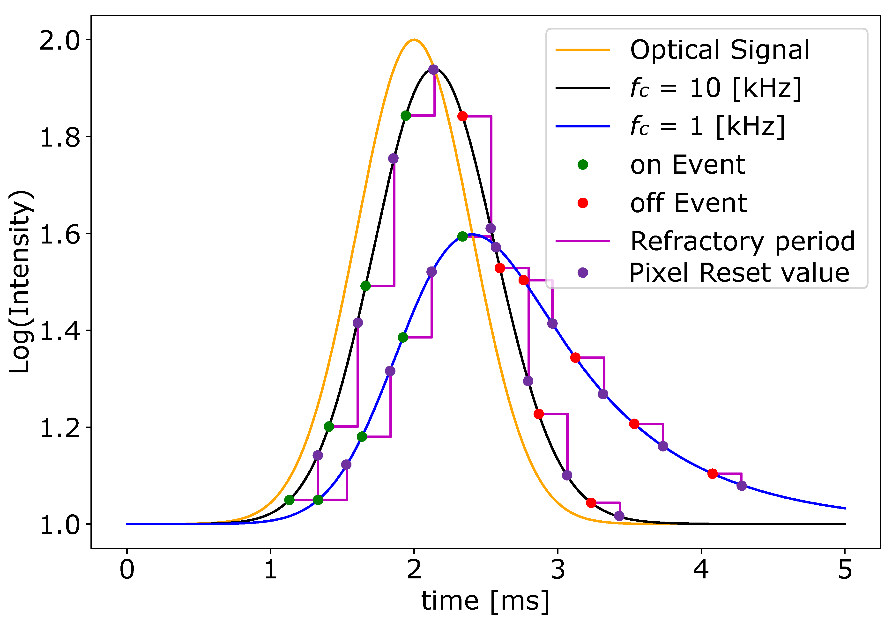
Figure 2.
(A) Relationship between bias_diff_on and bias_diff_off that produces similar event counts at a refractory period of 50 µs. Blue dots show the values used for threshold estimation, while the orange line show an exponential fit, enabling the user to match arbitrary on and off bias settings. (B) On (blue) and off (red) thresholds as a function of bias_diff_on. The results are based on a region of pixels including the brightest star in the field of view. The error bars are derived from the fitting results. The inset shows a logarithmic Gaussian (log-Gauss) fit used to estimate the peak event count at different bias settings. The x-axis indicates pixel indices.
Figure 2.
(A) Relationship between bias_diff_on and bias_diff_off that produces similar event counts at a refractory period of 50 µs. Blue dots show the values used for threshold estimation, while the orange line show an exponential fit, enabling the user to match arbitrary on and off bias settings. (B) On (blue) and off (red) thresholds as a function of bias_diff_on. The results are based on a region of pixels including the brightest star in the field of view. The error bars are derived from the fitting results. The inset shows a logarithmic Gaussian (log-Gauss) fit used to estimate the peak event count at different bias settings. The x-axis indicates pixel indices.
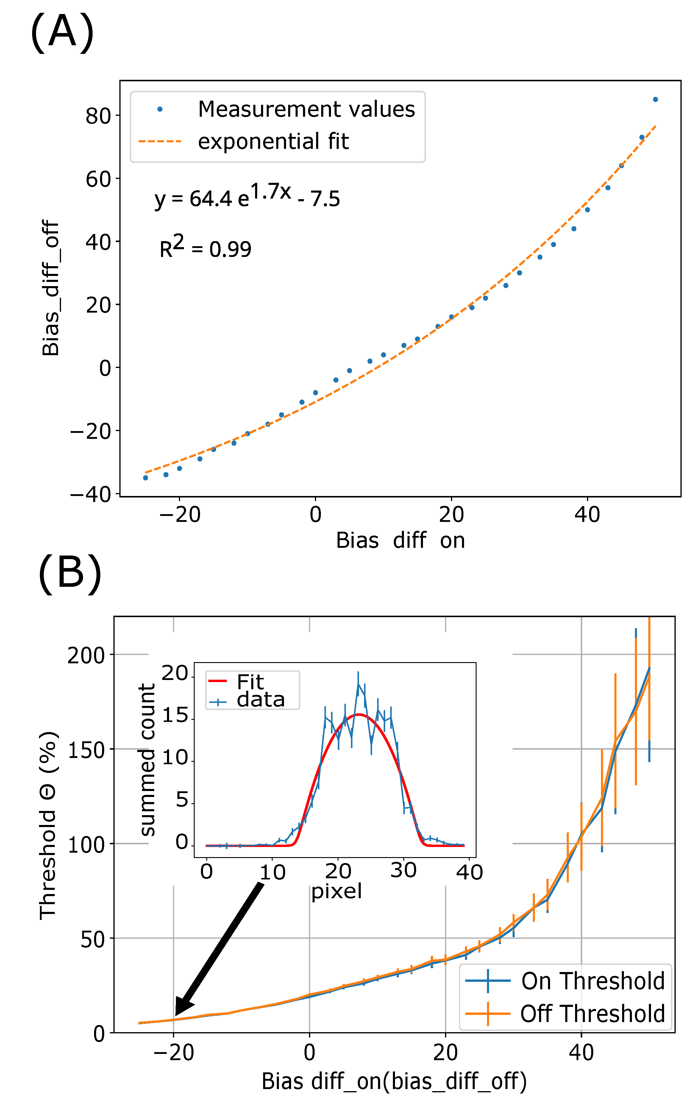
Figure 3.
(A) The refractory periods as a function of settings. The factory calibrated results from the Prophesee API function (orange) are shown in the figure for comparison. The errorbars are estimated from the timestamp resolution of the EVK4. (B) Measurements of refractory periods for two different bias_refr settings. The top panel show the fastest setting, where the refractory period is found to be 12 µs, whereas the bottom panel show the slowest setting with a refractory period of 480 µs.
Figure 3.
(A) The refractory periods as a function of settings. The factory calibrated results from the Prophesee API function (orange) are shown in the figure for comparison. The errorbars are estimated from the timestamp resolution of the EVK4. (B) Measurements of refractory periods for two different bias_refr settings. The top panel show the fastest setting, where the refractory period is found to be 12 µs, whereas the bottom panel show the slowest setting with a refractory period of 480 µs.
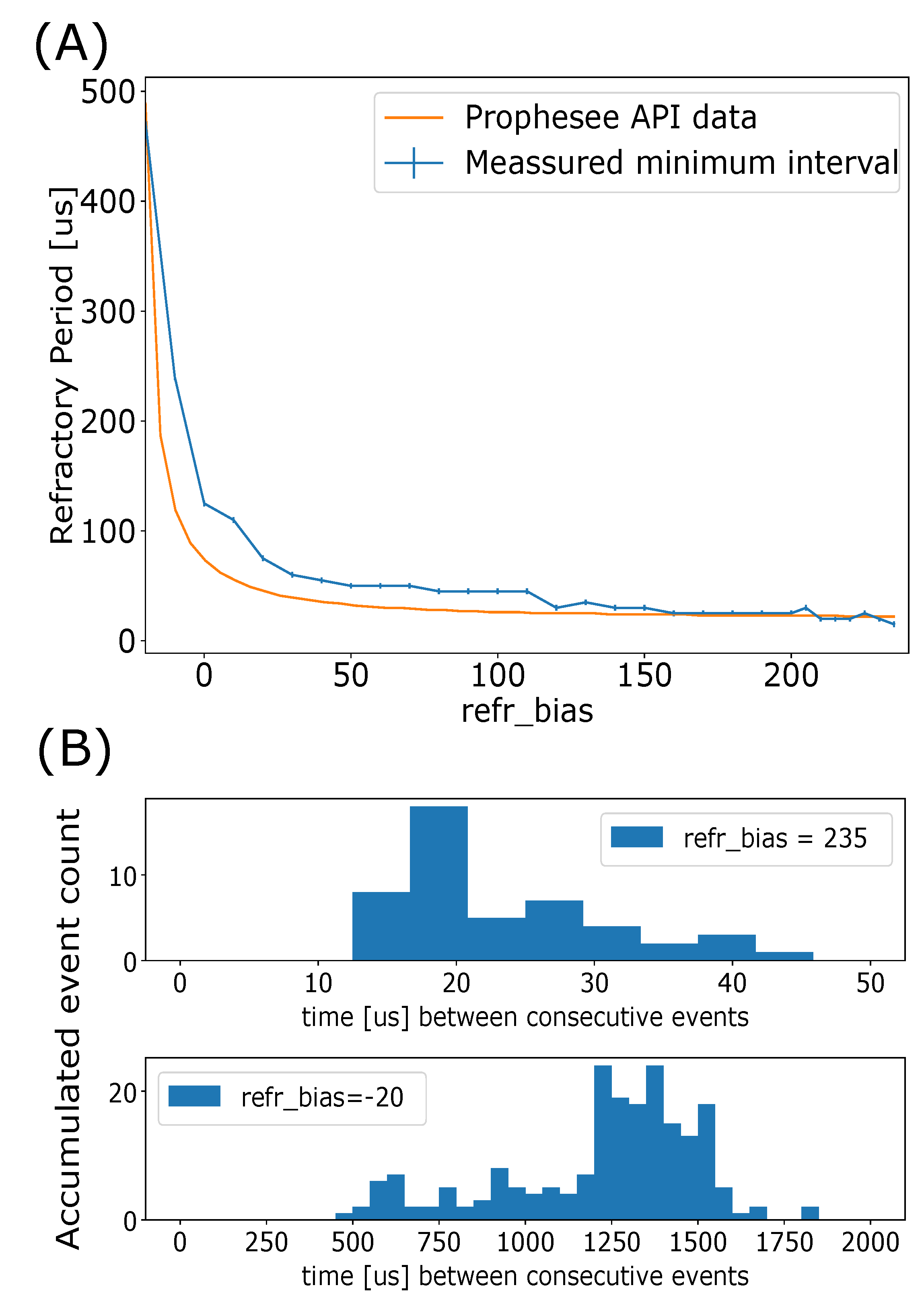
Figure 4.
Measurements of the corner frequency at different bias_fo settings for on (A) and off (B) events. As the frequency of the applied sine wave through the LED increases, the number of registered events decreases due to the low-pass filtering effect.
Figure 4.
Measurements of the corner frequency at different bias_fo settings for on (A) and off (B) events. As the frequency of the applied sine wave through the LED increases, the number of registered events decreases due to the low-pass filtering effect.
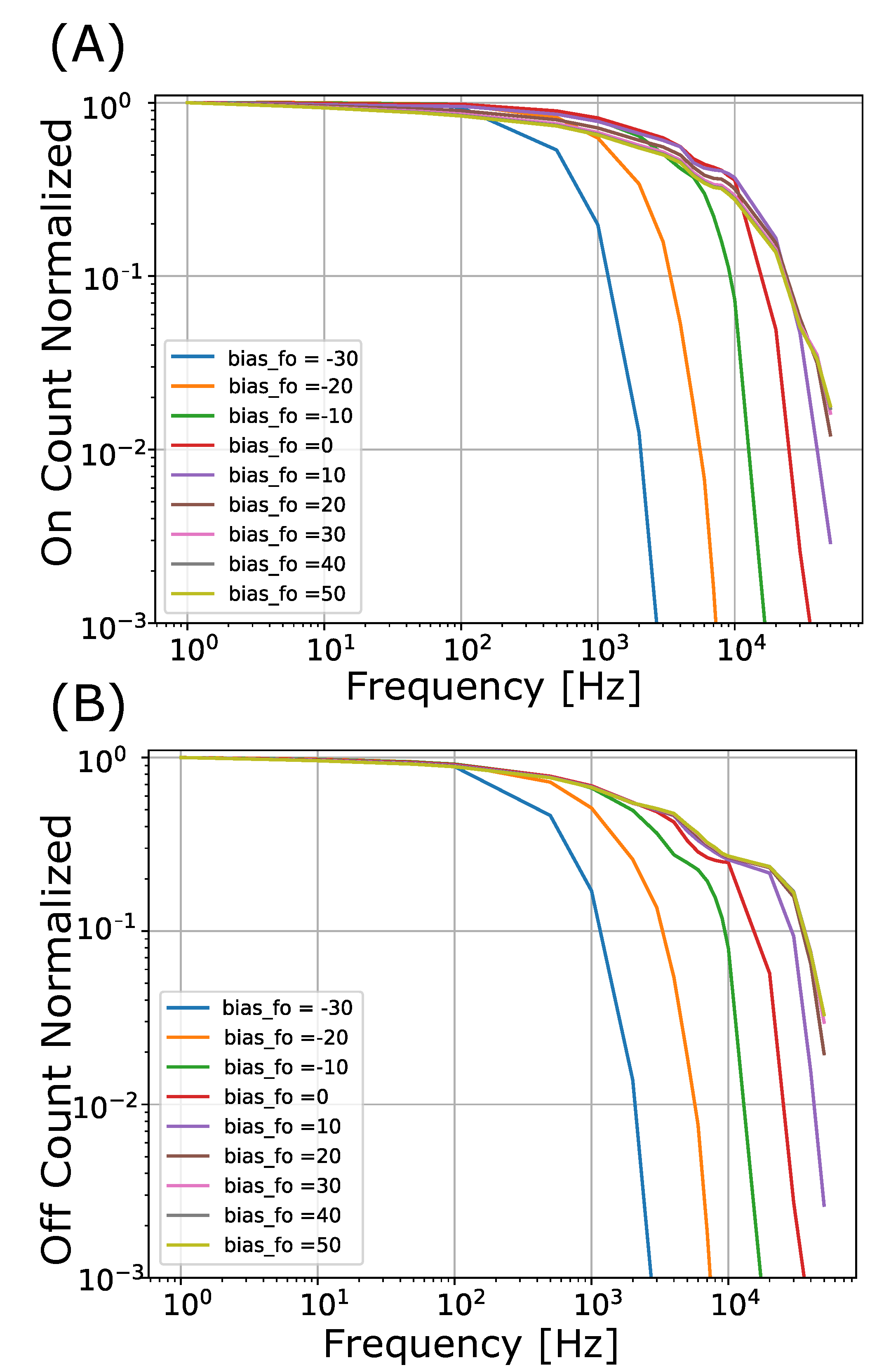
Figure 5.
Simulation of a single perfect pixel with no threshold mismatch and no effect from the refractory period with different against the measurement result (black) at bias_fo = 10. The horizontal dashed black line indicates the value where only a single On event is present per sine wave. For a single perfect pixel this is the lowest possible simulation value.
Figure 5.
Simulation of a single perfect pixel with no threshold mismatch and no effect from the refractory period with different against the measurement result (black) at bias_fo = 10. The horizontal dashed black line indicates the value where only a single On event is present per sine wave. For a single perfect pixel this is the lowest possible simulation value.
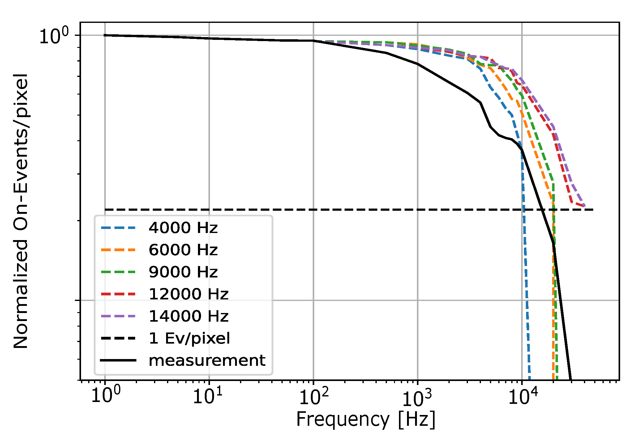
Figure 6.
Histogram of simulated (A) and measured (B) pixel response for a 100 Hz sine wave. These show the distribution of On events for a single cycle, highlighting that there is Threshold mismatch between pixels - leading to a distribution of event counts in different pixels. The distribution for the simulated pixels (A) match the measurement (B) when a random Gaussian error of is included for each pixel in the simulation.
Figure 6.
Histogram of simulated (A) and measured (B) pixel response for a 100 Hz sine wave. These show the distribution of On events for a single cycle, highlighting that there is Threshold mismatch between pixels - leading to a distribution of event counts in different pixels. The distribution for the simulated pixels (A) match the measurement (B) when a random Gaussian error of is included for each pixel in the simulation.
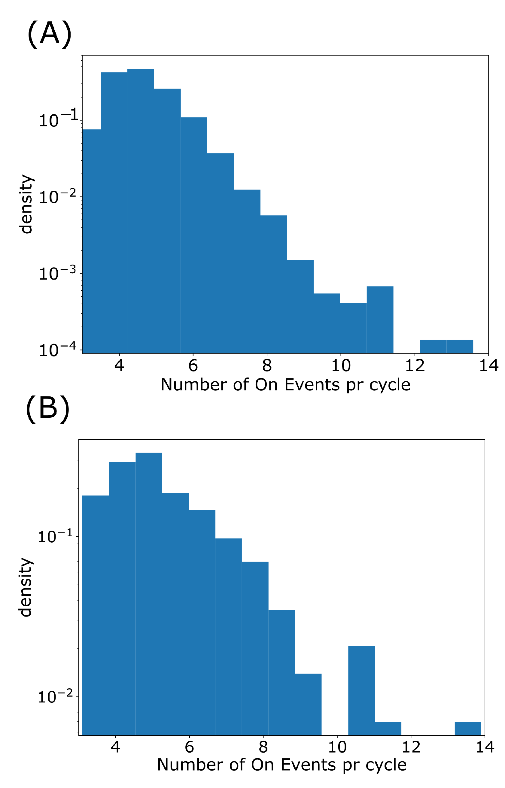
Figure 7.
(A) simulation of a single perfect pixel with no threshold mismatch and no effect from the refractory period with different against the measurement result (black) at bias_fo = 10. The horizontal dashed black line indicates the value where only a single On event is present pr sine wave. For a single perfect pixel this is the lowest possible simulation value. (B) bias_fo vs corner frequencies. The curve is obtained by finding the simulation frequencies with between measured and simulated results for a given bias_fo, with the same frequency for both on and off measurements. The errorbars are estimated from the distance between the simulated values used in each of the estimations. (C,D) Simulation of an area of pixels with threshold mismatch and the refractory period of 12 µs at different against the measurement result (black) at bias_fo = 10 for on and off events, respectively. Best match is at a corner frequency of 9000 Hz for both on and off events. (E,F) Residuals when comparing measured values with simulation, for On and Off events respectively.
Figure 7.
(A) simulation of a single perfect pixel with no threshold mismatch and no effect from the refractory period with different against the measurement result (black) at bias_fo = 10. The horizontal dashed black line indicates the value where only a single On event is present pr sine wave. For a single perfect pixel this is the lowest possible simulation value. (B) bias_fo vs corner frequencies. The curve is obtained by finding the simulation frequencies with between measured and simulated results for a given bias_fo, with the same frequency for both on and off measurements. The errorbars are estimated from the distance between the simulated values used in each of the estimations. (C,D) Simulation of an area of pixels with threshold mismatch and the refractory period of 12 µs at different against the measurement result (black) at bias_fo = 10 for on and off events, respectively. Best match is at a corner frequency of 9000 Hz for both on and off events. (E,F) Residuals when comparing measured values with simulation, for On and Off events respectively.
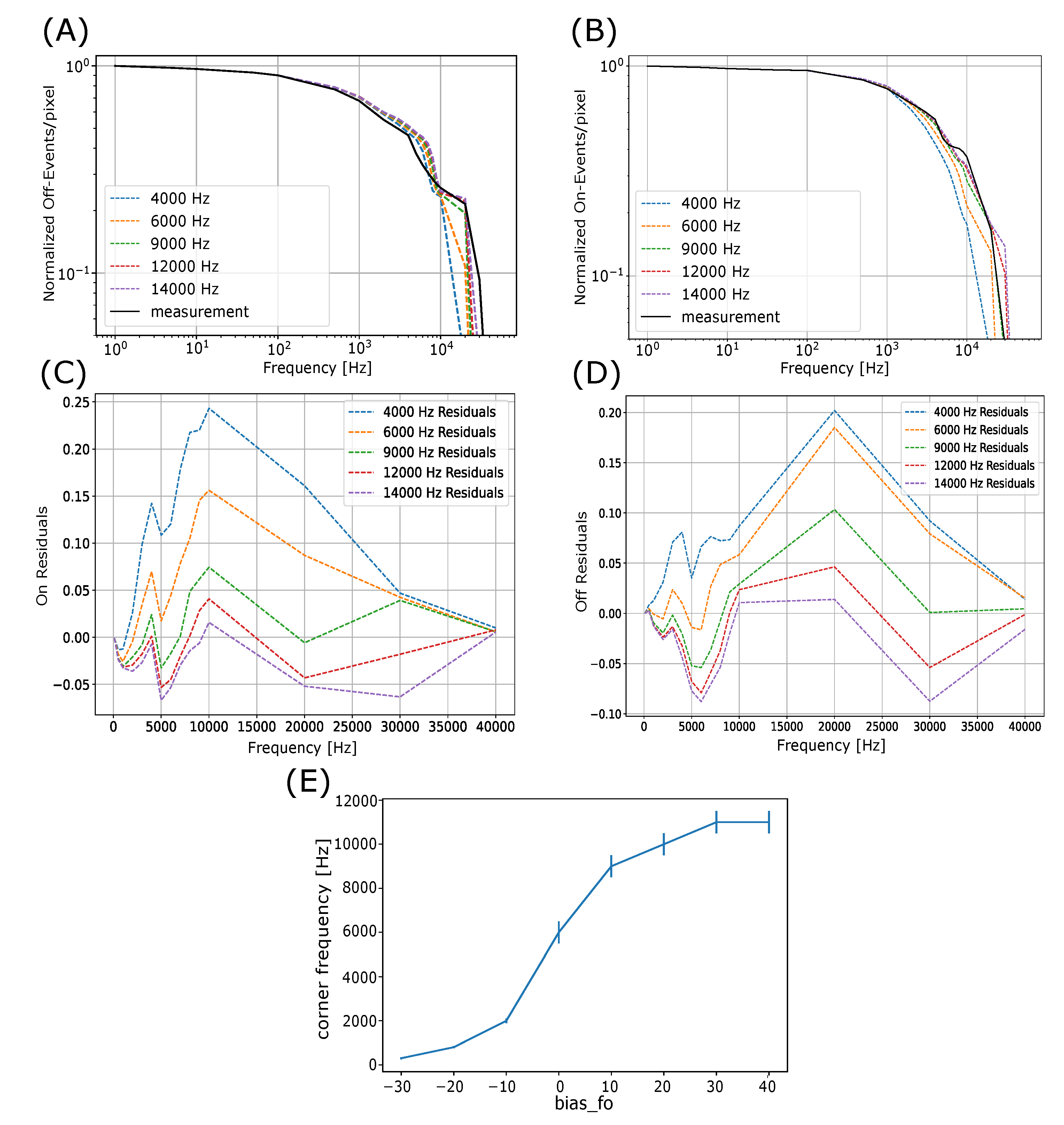

Table 1.
Bias settings for EVK4. The bias values appears as signed digital integer offsets relative to their factory-calibrated default values, defined as zero. Although these offsets do not have a direct physical interpretation, they modify the internal bias currents and thereby influence the sensor response. The performance of the camera as described in Section 3.
Table 1.
Bias settings for EVK4. The bias values appears as signed digital integer offsets relative to their factory-calibrated default values, defined as zero. Although these offsets do not have a direct physical interpretation, they modify the internal bias currents and thereby influence the sensor response. The performance of the camera as described in Section 3.
| Bias name | Minimum bias values | Maximum bias values | Effect |
|---|---|---|---|
| bias_diff_on | -85 | 140 | On-threshold |
| bias_diff_off | -35 | 190 | Off-threshold |
| bias_fo | -35 | 55 | Low-pass filter corner frequency |
| bias_refr | -20 | 235 | Refractory period (pixel dead time) |
Table 2.
Typical time constants for different physical phenomena and recommended bias settings. The bias_fo required to reach the suggested corner frequencies can vary if the steady state illumination of the process is much brighter than the physical phenomena mentioned here.
Table 2.
Typical time constants for different physical phenomena and recommended bias settings. The bias_fo required to reach the suggested corner frequencies can vary if the steady state illumination of the process is much brighter than the physical phenomena mentioned here.
| time constants | Physical Phenomena | Suggested bias values Threshold refr |
|---|---|---|
| Lightning streamer/corona | 12 µs | |
| Lightning Leader propagation | 12 µs | |
| Red Sprites | 12 µs | |
| Blue Jets | 40 µs | |
| Aurora | 80 µs |
Table 3.
The operating range for different bias settings.
| Bias name | Min. tested value | Max Tested value | Min. measured value | Max. measured value | Effect |
|---|---|---|---|---|---|
| bias_diff_on | -25 | 50 | On-threshold | ||
| bias_diff_off | -35 | 85 | Off-threshold | ||
| bias_fo | -30 | 50 | 1 kHz | 11 kHz | corner frequency |
| bias_refr | -20 | 235 | 12 µs | 480 µs | Refractory period |
Disclaimer/Publisher’s Note: The statements, opinions and data contained in all publications are solely those of the individual author(s) and contributor(s) and not of MDPI and/or the editor(s). MDPI and/or the editor(s) disclaim responsibility for any injury to people or property resulting from any ideas, methods, instructions or products referred to in the content. |
© 2026 by the authors. Licensee MDPI, Basel, Switzerland. This article is an open access article distributed under the terms and conditions of the Creative Commons Attribution (CC BY) license (http://creativecommons.org/licenses/by/4.0/).
Copyright: This open access article is published under a Creative Commons CC BY 4.0 license, which permit the free download, distribution, and reuse, provided that the author and preprint are cited in any reuse.