
Submitted:
13 August 2026
Posted:
17 August 2026
You are already at the latest version
Abstract
Car-sharing systems, as an important form of shared transport, face supply-demand imbalance and complex scheduling challenges. Heterogeneous vehicle can better meet diverse customer demands by offering vehicles with different capacities. Meanwhile, uncertainty in dispatcher movement time and vehicle relocation time may affect the reliability of scheduling plans. To address these issues, this paper focuses on a one-way station-based car-sharing problem, considering integrated scheduling, heterogeneous vehicle, uncertain dispatcher movement time and vehicle relocation time simultaneously. We define the uncertainty sets for dispatcher movement time and vehicle relocation time based on historical data from the Taxi & Limousine Commission (TLC) in Queens, New York by data-driven method. A robust optimization model is developed to improve order fulfillment and scheduling stability. We develop a hybrid approach that combines adaptive large neighborhood search and a genetic algorithm (ALNS/GA), and incorporates robustness into solution decoding and fitness evaluation under the data-driven uncertainty sets. Numerical experiments based on real TLC data show that the integrated scheduling system reduces average costs by 10.69\% compared with non-integrated systems, while the integrated robust scheduling system further improves the order fulfillment rate by 0.99\%. Sensitivity analysis also offers useful managerial insights.
Keywords:
car-sharing
; uncertainties
; robust optimization
; heterogeneous vehicle
1. Introduction
Car-sharing transportation, as a typical example of shared transportation (see Figure 1), has become an important travel mode for urban residents [1]. The global car-sharing market is estimated at USD 11.52 billion in 2025 and is projected to reach USD 28.67 billion by 2030, corresponding to a CAGR of 20.0% over 2025–2030 [2]. Car-sharing offers novel solutions to urban transportation challenges like traffic congestion, taxi availability issues, and parking difficulties [3]. Additionally, it ensures a comparable level of travel comfort to private vehicles [4]. Car-sharing services come in two main types: station-based and free-floating. In densely populated cities, there will be little parking space and high parking costs, which will limit the service capacity of free-floating systems [5]. Within the station-based model, services can be further classified as either one-way or round-way. Consumers are increasingly prioritizing comfort and convenience, causing the traditional round-way model to lose its attractiveness gradually [6].
However, one-way station-based car-sharing services may face a spatial mismatch between vehicle availability and customer demand [7]. (i) How to address this imbalance through the development of effective scheduling plans? In practical operations, uncertainty in both dispatcher movement time and vehicle relocation time may prevent scheduling plans from being executed accurately, thereby affecting the stability of order fulfillment. In the long run, ensuring order fulfillment rates and subsequently improving customer satisfaction are key to establishing a competitive advantage for the car-sharing platform [8]. So, (ii) how can scheduling plans maintain good performance in the face of uncertainty? Additionally, (iii) how can a car-sharing system be designed to meet diverse customer demands and provide personalized services?
To develop effective scheduling plans that address supply-demand imbalances, vehicle relocation becomes a key factor influencing the performance of these plans. Vehicle relocation determines which vehicle should be moved from its supply location to its demand location. This process is relatively complex because, unlike other small-scale shared mobility systems like bicycles, vehicles cannot be moved in bulk on a single carrier [9]. Therefore, the process of relocating vehicles necessitates dispatchers driving them to the demand station. Dispatchers can move around the station where the vehicle is located by folding bicycles, scooters [10], public transport [11] or shuttle vehicles [9]. In order to address supply-demand imbalances, integrated scheduling plans are required to simultaneously coordinate order allocation, vehicle relocation and dispatcher movement.
In practical operations, both dispatcher movement time and vehicle relocation time can be influenced by various subjective and objective factors, such as individual riding/driving proficiency, weather conditions, road congestion, and excessive traffic lights, resulting in variability in execution time [12]. Utilizing deterministic models may not offer effective scheduling plans to meet customer demands. To address uncertainties, researchers often turn to methods such as stochastic programming. However, stochastic programming has its limitations, particularly in determining the data distribution of uncertain parameters. This becomes especially challenging when dealing with large-scale problems and high-dimensional historical data. Robust optimization handles time uncertainty by optimizing decisions against the worst-case realization in a prescribed uncertainty set, while a small set of protection parameters controls the level of conservatism [13]. With the growing availability of operational data, uncertainty sets can be calibrated directly from historical observations within a data-driven robust optimization framework. In this paper, we develop a data-driven interval uncertainty set from historical records of the Taxi & Limousine Commission (TLC) in Queens, New York, by estimating bounds for dispatcher movement time and vehicle relocation time, and use a budget parameter to cap how many time components can simultaneously take their worst-case values under this set. Therefore, data-driven robust optimization produces integrated schedules that are less sensitive to travel-time disruptions, leading to more stable execution and higher order-fulfillment rates in practice.
The growing diversity of travel demands has encouraged car-sharing platforms to offer heterogeneous vehicle services [14]. While most studies assume a homogeneous fleet, real-world fleets are mixed, and ignoring heterogeneity can distort assignment and relocation decisions. In this paper, we model vehicle heterogeneity by categorizing vehicles based on seating capacity, considering three types: 2-seat, 5-seat, and 7-seat vehicles, which serve solo/couple, small-group, and larger family/group trips, respectively. Accordingly, each order must be served by a vehicle whose capacity is no smaller than the requested number of passengers [15]. By determining the appropriate fleet size, the quantity of different vehicle types and the allocation of vehicle tasks, the overall cost can be minimized [16]. In summary, this paper investigates an integrated robust scheduling system for one-way station-based car-sharing with heterogeneous vehicles to meet customer demands. The main contributions of this paper are as follows:
(1) To the best of our knowledge, in the domain of one-way station-based car-sharing, we first integrate the issues of order allocation, vehicle relocation, dispatcher movement, uncertain dispatcher movement time and vehicle relocation time into the problem;
(2) We consider a heterogeneous vehicle fleet, where 2-seat vehicles are for solo/couple, 5-seat for small groups, and 7-seat for larger family/group trips, to better meet diverse customer demand within the integrated scheduling framework;
(3) Based on analysis of historical data from TLC that is similar to this problem, uncertainty sets for dispatcher movement time and vehicle relocation time are defined in interval form by a data-driven method. Specifically, a robust optimization model that can be solved quickly and effectively is proposed to improve order fulfillment rate and the stability of integrated scheduling plans.
The remainder of the paper is organized as follows. Section 2 reviews the related literature. Section 3 describes the one-way station-based car-sharing setting and formulates the integrated scheduling problem. Section 4 presents the deterministic MILP and its data-driven robust counterpart under uncertain dispatcher movement and vehicle relocation time. Section 5 designs a hybrid algorithm for robust models, denoted as ALNS/GA. Section 6 reports numerical experiments, including scenario comparisons and sensitivity analyses. Section 7 concludes the paper and discusses limitations and future research directions.
2. Literature Review
2.1. Vehicle Relocation and Dispatcher Activity
Relocation tasks can be performed either directly by customers [3] or by the service provider [17]. In customer-based relocation, the platform offers incentives to induce users to relocate vehicles toward stations that alleviate distribution imbalances [18]. Zhang et al. [3] implement this idea through price discounts that encourage customers to return vehicles to desired locations. In practice, however, the realized effect of customer-based relocation may vary with users’ willingness to participate and respond to incentives [19]. Consequently, many operators also rely on provider-based relocation, where the platform transfers vehicles from surplus locations to shortage locations to restore balance [17]. Li et al. [20] illustrate that operator-based relocation is frequently embedded in daily operations to mitigate imbalances in vehicle availability. Xu and Wu [21] further refine this operator-based perspective by explicitly modeling how relocation actions reshape vehicle availability over space and time.
Early service-provider studies often model relocation mainly from the vehicle side and focus on deciding where vehicles should be moved, while leaving dispatcher activity implicit [11]. In practice, however, operator-based relocation must be carried out by dispatchers: a dispatcher needs to travel to the pickup station, take the vehicle, and drive it to a shortage station. These steps consume time and dispatcher resources, so a relocation plan that ignores dispatcher activity may be difficult to implement [22]. Yu et al. [23] include dispatcher-based relocation as part of the rebalancing design, indicating that platform relocation still relies on dispatchers to move vehicles in daily operations. Guo et al. [6] then point out a basic requirement: to relocate vehicles, dispatchers must also travel between stations, and this travel affects whether a relocation plan is feasible and how good it is in practice. Bruck et al. [24] state the same idea in a bike-sharing setting and draw a direct implication for modeling: a rebalancing plan should specify dispatcher routes and station-to-station travel, not only the target vehicle distribution. Therefore, vehicle relocation and dispatcher activity should be considered jointly in daily operations.
Some studies integrate vehicle relocation and dispatcher activity, achieving rebalancing of car-sharing system by dispatchers to drive vehicles from surplus stations to shortage stations [6]. Wu et al. [25] consider four types of travel arcs for dispatchers, including waiting, maintenance, movement, and relocation. Yang et al. [26] categorize vehicle travel arcs into three types: parking, user driving, and dispatcher relocating. Tian et al. [27] formulate vehicle relocation and dispatcher rebalancing as a joint operational problem in a one-way free-floating car-sharing system and construct relocation plans by assigning vehicle relocation tasks to dispatchers in a way that respects dispatcher availability and station-to-station travel. Guo et al. [28] integrate vehicle rebalancing with operational relocation effort by jointly optimizing charging schedules and inter-station relocation decisions. From a routing perspective, Gleditsch et al. [29] generate executable operator tours for dynamic rebalancing, linking relocation quantities to feasible routes and the resulting visiting sequence of locations. In recent studies, dispatcher movement between stations is typically realized by small personal devices such as folding bicycles, scooters, public transport or shuttle vehicles. Chang et al. [10] model dispatcher movement by allowing dispatchers to use a folding bicycle or an electric scooter to travel to the next relocation task. Eilertsen et al. [11] allow dispatchers to move between tasks by either a folding bicycle or public transport. Liu et al. [9] model dispatcher movement through dedicated shuttles that transport dispatchers between stations.
2.2. Uncertain Factor
There is relatively limited research on uncertainties in car-sharing systems, with most studies focusing on demand uncertainty and employing stochastic or multi-stage methods. Specifically, Oliveira et al. [30] incorporate a choice-based demand model into operator decisions, providing a structured way to represent demand variability when optimizing relocation actions. Zhang et al. [3] formulate a two-stage stochastic programming model under uncertain demand and derive operator relocation plans to mitigate supply–demand imbalances. Basciftci et al. [14] develop a two-stage stochastic mixed-integer program that integrates multi-period planning decisions with operational relocations under demand uncertainty. In summary, some studies mainly consider demand uncertainty, while less attention has been paid to other factors that may affect the operational efficiency of car-sharing systems, such as dispatcher movement time and relocation travel time.
Robust optimization has been increasingly applied to address uncertainty in scheduling problems [31]. Compared to traditional methods that rely on inputs with random distributions, robust optimization minimizes input requirements and enhances model versatility to tackle challenges like the curse of dimensionality and limited historical data [32]. In shared-mobility rebalancing, Bruck et al. [24] formulate rebalancing as a robust optimization problem and show that robust counterparts can still be solved exactly with tailored algorithms. Chen et al. [33] incorporate distributional robustness into free-floating bike rebalancing, so that the resulting plan is less sensitive to demand perturbations. Zhang et al. [34] push this direction further by calibrating the uncertainty description from historical observations and embedding it in a multi-period robust repositioning model. Beyond demand-side uncertainty, execution-time uncertainty is also crucial in shared mobility, and it has been increasingly incorporated into routing and operational optimization models [35]. Time uncertainty has also been treated explicitly in robust routing models, where uncertain travel times are embedded into the feasibility requirements of time-dependent constraints [36]. In a real-time dispatch-and-relocation setting, Chen et al. [37] handle travel-time uncertainty through a distributionally robust chance-constrained formulation while making vehicle relocation decisions online. Overall, although time uncertainty has been increasingly considered in shared-mobility operations, robust car-sharing scheduling still rarely models uncertainty in vehicle relocation time or in dispatcher movement time, and studies that consider both simultaneously are even rarer.
2.3. Research Gap
Table 1 summarizes the features of previous research efforts. The distinctions of this study from previous research are as follows: Firstly, References [8,21,23,24,25,28,29,32,33] are similar to this study as they also address the dual scheduling of one-way station-based car-sharing system. However, these studies all adopt deterministic models, without considering the uncertainties in real-world scenarios. Secondly, References [3,22,26,34,39] address the uncertainty of customer demands but do not tackle integrated scheduling problem involving both vehicles and dispatchers. To our knowledge, there is currently no research that simultaneously considers the uncertainty in dispatcher movement time and vehicle relocation time, or integrates such uncertainties into the integrated scheduling problem. Thirdly, although the importance of heterogeneous fleets has been studied in the fields of VRP and LRP, it has only received some attention in the domain of car-sharing in recent years. Smet [38] investigates a car-sharing system with heterogeneous fleets, where customers are assigned to alternative vehicles when the requested vehicle type is unavailable. However, this study is limited to a round-way scenario and does not consider vehicle relocation. Based on the above comparison, few studies in one-way station-based car-sharing simultaneously integrate scheduling, a heterogeneous fleet, and uncertainty in both dispatcher movement time and vehicle relocation time.
3. Problem Description
3.1. System Setting
Consider a station-based car-sharing system for one-way rentals where customers provide booking details such as start time, end time, departure station and destination station. We define the start time, end time, departure station and destination station for each demand as , respectively. The car-sharing platform offers heterogeneous vehicle services with known types and quantities. The location and number of stations are predetermined, each station with limited capacity. Each service-providing vehicle may not necessarily start its next task from the destination station it arrived at after completing the previous one. Failure to meet customer demands incurs penalty costs. This heterogeneity in service leads to significant spatial imbalance between vehicle availability and customer demands. Therefore, dispatchers are required to ride scooters between stations, and relocate vehicles to meet demands and address imbalance issues. Dispatchers begin executing tasks from their initial stations at the start of scheduling and return to those stations by the end of scheduling. We name the problem as car-sharing integrated scheduling with heterogeneous fleet, abbreviated as CISH for later references.
The topology of the one-way station-based car-sharing system can be described using a time-space network, where nodes correspond to stations at different points in time, and arcs denote the interactions involving customers, vehicles, and dispatchers. There are three types of activities in the system: travel, relocation and movement. Travel refers to customers using vehicles through the system. Relocation involves dispatchers driving vehicles between stations. Movement refers to dispatchers riding scooters from one station to the station where relocation tasks need to be executed.
Figure 2 illustrates the integrated scheduling process of the entire car-sharing system. Initially, orders are allocated to vehicles based on customer request information. As imbalances arise between customer demand and vehicle availability, the algorithm integrates customer departure times, pick-up station, drop-off station, the current location of dispatchers and vehicles to calculate potential relocation arcs. Integrated scheduling involves order allocation, vehicle relocation and dispatcher movement. Vehicle relocation routes contain 2-3, 4-5, 7-8, 9-10, 11-6, 13-10 and 14-15. The initial stations with three dispatchers are 1, 6, and 12. The movement routes are 3-4, 8-9, 10-11 and 10-14. The dummy arcs for dispatcher departures and returns from stations are as follows: 1-2, 5-1, 6-7, 12-13, and 15-12. Taking the first dispatcher as an example, he departs from station 1 to supply station 2 and drives the required vehicle to demand station 3. Then, he rides a scooter to supply station 4 and delivers the required vehicles to station 5. Finally, he completes all tasks and returns to his starting point. Each dispatcher is assigned a unique initial station, which serves as the dispatcher’s departure and return location during the scheduling horizon. These initial stations do not undertake any demand-related tasks to maintain the structural clarity of the scheduling model. Figure 3 complements Figure 2 by showing how integrated scheduling decisions translate into executable time sequences for individual dispatchers. Each panel decomposes the execution time into dispatcher movement, vehicle relocation, and the customer-service interval. For task 1, dispatcher 1 performs a direct vehicle relocation from station 4 to station 1, followed by the customer-service segment. For task 2, dispatcher 2 first moves from station 3 to station 4 and then relocates a vehicle from station 4 to station 1; the movement segment, relocation segment, and customer-service segment are displayed separately to reflect their temporal order. By accounting for these execution-time components, the integrated schedule better matches vehicles to bookings, improving order fulfillment and service reliability of the car-sharing system.
3.2. Time Discretization for Data-Driven Uncertainty Sets
To formalize the above operations on the time–space network and ensure temporal consistency in subsequent order allocation, vehicle relocation, and dispatcher movement, we discretize the planning horizon as follows [39]. We consider a scheduling horizon and discretize it into equal-length periods of minutes. Let denote the set of discrete time indices, where
Here is the real clock time corresponding to index t. The discrete time indices are used to map customer trips, construct candidate scheduling arcs, and update station inventories over the planning horizon. The exact start times of dispatcher tasks remain continuous and are measured in minutes to preserve scheduling accuracy. To avoid constructing arcs that leave the planning horizon, we only allow new customer trips, vehicle relocations and dispatcher movements to depart from periods . The last period is used solely to complete ongoing tasks and record the final inventories at stations.
For each demand , the booking data provide a continuous start time , a continuous end time , a departure station , and a destination station . The continuous times are mapped to discrete period indices by
In this way, represents the earliest period in which demand c can start using a vehicle, and represents the latest period by which the vehicle must be returned. Therefore, the continuous time interval is fully contained in the discrete interval . Hence, each customer travel task is represented by a fixed travel arc in the time–space network.
Given the nominal relocation time and movement time between stations i and j, their discrete counterparts in periods are defined as and , respectively. A time–space arc is constructed if departing from station i at period t reaches station j at
which guarantees that all arcs in the network are aligned with the discrete time grid.
Note that t and k are indices of coarse time periods, while and are continuous-time durations (in minutes). Dividing by converts a duration into the number of periods it spans. The ceiling operator guarantees temporal feasibility on the coarse time axis, i.e., the actual arrival time (or ) always falls no later than the end of period k.
It is worth noting that the proposed model adopts a two-scale representation of time. Coarse-grained time indices are used to construct the time–space network and enforce vehicle inventory balance at stations. In contrast, the continuous scheduling variables , and are defined in minutes to capture the finer dispatching sequence of relocation tasks within each period. This two-layer time structure allows us to keep the network size tractable while retaining sufficient temporal resolution for dispatcher scheduling.
For the budget uncertainty sets introduced later, we adopt a rolling window with physical length W minutes, corresponding to consecutive periods. For each , the associated window is defined as
Hence, the budget parameter controls the maximum number of periods that may simultaneously attain worst-case deviations within each window .
4. Model
In this section, we first formulate a deterministic mixed-integer linear programming (MILP) model for the CISH. We then construct data-driven budgeted interval uncertainty sets for vehicle relocation time and dispatcher movement time. Based on these sets, the deterministic model is reformulated into its robust counterpart by robustifying the key temporal-feasibility constraints and the generalized operating-cost objective via standard dual reformulation.
4.1. Deterministic Model of CISH
4.1.1. Notations
Sets
| C | Set of customer demands |
| S | Set of dispatchers |
| T | Set of discrete time periods, |
| I | Set of stations |
| H | Set of vehicle types |
| Set of vehicle types suitable for customer demand , | |
| A | Set of all potential vehicle-relocation arcs |
| Set of arcs through which dispatcher s departs from the initial station | |
| Set of arcs through which dispatcher s returns to the initial station | |
| Set of all relocation arcs associated with dispatcher s, where | |
| Set of potential relocation arcs and initial departure arcs for dispatcher s, where | |
| Set of potential relocation arcs and terminal return arcs for dispatcher s, where | |
| a | Time–space arc , representing a route that departs from station i in period t and arrives at station j in period k. Similarly, , , and |
Indices and parameters
| Indices for stations | |
| Indices for time | |
| c | Index for customer demands, |
| s | Index for dispatchers, |
| h | Index for vehicle types, |
| Capacity of station i | |
| Nominal relocation time (minutes) for moving a vehicle from station i to station j | |
| Nominal movement time (minutes) for a dispatcher moving from station i to station j | |
| Discrete vehicle relocation duration (in periods) from station i to station j, defined as | |
| Discrete dispatcher movement duration (in periods) from station i to station j, defined as | |
| Penalty for abandoning a customer demand | |
| Vehicle relocation cost per unit time | |
| Cost of vehicle relocation by a dispatcher per unit time | |
| Dispatcher movement cost per unit time | |
| Initial number of vehicles of type h at station i | |
| M | A sufficiently large number |
| Fixed cost of a vehicle of type h | |
| Discrete start-period index of demand c, mapped from | |
| Discrete end-period index of demand c, mapped from | |
| Departure station of demand c | |
| Destination station of demand c | |
| Length of each discrete time period (minutes) used to discretize the planning horizon | |
| Clock time corresponding to discrete index t, i.e., , | |
| W | Physical length (minutes) of the rolling time window in the budgeted uncertainty sets, which induces consecutive periods |
| Number of vehicles of type h at station in period |
Decision variables
| Binary variable equal to 1 if customer demand c is served by a vehicle of type h, and 0 otherwise | |
| Binary variable equal to 1 if dispatcher s relocates a vehicle of type h along relocation arc , and 0 otherwise | |
| Binary variable equal to 1 if dispatcher s relocates a vehicle of type h along arc and subsequently relocates a vehicle of type along arc , and 0 otherwise | |
| Number of vehicles of type h relocated along arc | |
| Starting time (minutes) at which dispatcher s begins the relocation task along arc |
4.1.2. Model Composition
The deterministic model of CISH is formulated as follows.
Objective function: The minimization objective function includes the penalty cost of unmet demands, vehicles and dispatchers relocation cost, dispatchers movement cost, and the fixed cost of vehicles h used to meet demand in operation hours, which are collectively referred to as generalized daily operating costs.
where in the dispatchers movement cost is the dummy relocation of dispatchers from and to the depot.
Flow conservation: The available vehicles at station i at time is calculated as follows: it equals the number of available vehicles at time t plus the vehicles that arrived at station i during the interval , minus the vehicles that departed from station i during the interval , plus the vehicles relocated to station i and minus those relocated from station i during the same interval. We assume that no travels, relocations, or movements occur at the final time .
Vehicles and stations: Constraint (3) ensures that, for each vehicle type h, the number of type-h vehicles available at station i at time t, together with the type-h vehicles relocated to station i at time t, is no less than the total number of type-h vehicles that are assigned to customer trips or relocation tasks departing from station i at time t. Constraint (4) ensures that each demand is allocated to at most one type of vehicle. Constraint (5) states that at any given time, the number of vehicles at each station must not exceed the station’s capacity.
Scheduling: Constraint (6) states that relocation tasks are performed exclusively by dispatchers, hence the number of times vehicles are relocated equals the number of relocation tasks executed by dispatchers. Constraints (7) and (8) ensure that if dispatcher s does not perform a relocation task on arc a, then any relocation task on arcs connected to this arc, either preceding or succeeding it, cannot be executed. Constraint (9) ensures that for dispatcher s, performing a relocation task on arc must be preceded by execution of a connected arc a; in other words, each relocation task cannot occur independently and must be linked to a preceding arc. Constraint (10) ensures the flow balance of dispatchers, requiring that for each dispatcher, the number of relocation flows departing from arc a equals the number of relocation flows entering it. Constraint (11) specifies that the start time for relocating vehicles on arc by a dispatcher should be greater than or equal to the start time for relocating vehicles on arc a, plus the relocation time from i to j, and the time it takes the dispatcher to move from j to . Constraint (12) is similar to constraint (11) but applies to dummy relocation arcs. Since the end station of a dummy relocation arc coincides with the start station of the subsequent relocation task, only the dispatcher’s movement time between arcs is considered, and the vehicle relocation time is excluded. Constraints (13) and (14) ensure that each dispatcher departs from their initial station at the start of scheduling and returns to the initial station at the end of scheduling.
Time window: Constraint (15) is the time window constraint for dispatcher s to perform the relocation task on arc a departing from station i. It ensures that the start time must lie within the bounds defined by the earliest and latest feasible start times, and , respectively. Specifically, denotes the earliest possible start time (in minutes) of the relocation task on arc a, determined by the dynamic scheduling requirements, whereas denotes the latest possible start time.
Variables: Constraints (16)-(18) restrict that and are binary variables. Constraints (19)-(22) define that and are integer variables.
4.2. Robust Counterpart for CISH
4.2.1. Uncertainty Set Construction
In real-world operations, the relocation time of dispatchers is subject to various sources of uncertainty, including traffic congestion, dynamic route changes, unexpected detours, and heterogeneous driving proficiency. As a result, the actual relocation time may deviate from its nominal estimate and exhibit time-varying fluctuations. Following the data-driven budgeted-uncertainty-set framework of literature [40], we construct a budget-based uncertainty set over a rolling time window , which consists of consecutive periods from t to .
Specifically, for each window starting at t, the interval bounds and the associated budget parameters are calibrated from historical observations and can be updated in a rolling-horizon manner, while the robust optimization problem solved at t treats these calibrated quantities as given inputs. The uncertainty set is formulated as follows:
(1) For each period , is the interval support of the uncertain relocation time .
(2) and are the mean and the half-interval length of , respectively.
(3) is used to control the conservatism of the uncertainty set, representing the cumulative budget of uncertainty.
In real-world scenarios, dispatchers move by scooter, which may be influenced by multifarious factors such as road congestion, weather conditions, excessive traffic lights, unclear endpoint locations and other subjective and objective factors, leading to changes in movement time. Consequently, the actual movement time may deviate from the expected value, exhibiting a certain degree of volatility. We model the dispatchers’ movement time as a budget-type uncertainty over the same rolling window :
(1) For each period , is the interval support of the uncertain movement time .
(2) and are the mean and the half-interval length of , respectively.
(3) is used to control the conservatism of the uncertainty set, representing the cumulative budget of uncertainty.
4.2.2. Robust Counterparts of Constraints
Proposition 1. Constraint (11) can be reformulated as constraint (25).
Proof. Given the current period t, for each end period we consider the sub-horizon . Within the uncertainty set in Eq. (23), we define the scaled deviations for each as
Similarly, for the movement-time uncertainty set in Eq. (24), the scaled deviations are
Restricted to the sub-horizon , the sets and can be equivalently written as
Therefore, constraint (11), , is equivalent to the following inequality
To obtain the robust counterpart, we maximize the deviation terms on the left-hand side. Introducing the auxiliary quantities
Inequality Eq. (28) can be conservatively rewritten as
Dual reformulation. Following the dualization approach of Bertsimas and Sim [41], we introduce dual variables for the relocation time, and for the movement time. The dual forms of Eq. (29) and Eq. (30) are:
Substituting these dual forms into constraint (31) yields the linear robust counterpart of constraint (11):
The associated feasibility constraints of the dual variables are:
Thus, constraint (11) is replaced by its robust counterpart Eq. (34), ensuring that the temporal scheduling between consecutive relocation arcs remains feasible under any realization of uncertain relocation and movement times within their respective budget uncertainty sets.
Proposition 2. The robust dual linearized form of constraint (12) under the budget-based uncertainty set of dispatcher movement time is given as constraint (36).
Proof. Given period t and end period , we again restrict in Eq. (24) to the sub-horizon and define the scaled deviations as
The set is represented equivalently by the following inequality.
Therefore, constraint (12), is equivalent to the following inequality
By maximizing the deviation term on the left-hand side, we obtain the auxiliary maximization problem:
Dual reformulation. Following the dualization approach of Bertsimas and Sim [41], by introducing the dual variables , the dual form of the auxiliary problem is obtained as:
Substituting the dual expression of into constraint (38) yields the linearized robust dual constraint (41), that is:
together with the dual variable constraints
This completes the robust dualization of constraint (12), ensuring temporal feasibility between successive virtual arcs under any realization within the uncertainty set .
4.2.3. Robust Counterpart of the Objective Function
In addition to the temporal feasibility constraints, the relocation time and dispatcher movement time also appear in the generalized daily operating cost Eq. (1) as coefficients of e, y, and z. Hence, we further robustify the objective under the same rolling-window budget uncertainty sets and .
Proposition 3. Under the rolling-window budget uncertainty sets and , the robust counterpart of the objective function Eq. (1) admits the following equivalent linear reformulation:
subject to the exposure-defining constraints
where for an arc , we define , , and .
The dual variables satisfy the following feasibility constraints:
All dual variables satisfy the following nonnegativity constraints:
Proof.
Following the scaled-deviation representation in Proposition 1–2, for each fixed and window starting at t, we write and , where , , and , for all .
Here, and collect the decision-dependent exposure terms and are defined in constraints (44) and (45). Substituting the midpoint–deviation representations into Eq. (48) separates the objective into a nominal part and a deviation part. For each fixed , the deviation part leads to the following two auxiliary maximization problems:
Dual reformulation. Following the same dualization approach of Bertsimas and Sim [41] used in Proposition 1–2, introduce dual variables for , and for . Their dual-feasibility conditions are exactly constraint (46), and the corresponding dual objective values yield the additional linear terms
in the outer minimization. Summing over all and combining with the nominal part completes the derivation, leading to the linear robust objective Eq. (43) with constraints (44)–(46).
Combining Proposition 1–3, the robust dual form of the car-sharing integrated scheduling problem is a mixed-integer linear programming model obtained by minimizing Eq. (43) subject to constraints (2)–(10), constraints (13)–(22), the robust scheduling constraints (25) and (36), and the robust-objective constraints (44)–(46).
5. Solution Method
The car-sharing integrated robust scheduling problem yields a large and highly constrained search space, and its difficulty grows rapidly with the fleet size. Moreover, execution-time uncertainty in vehicle relocation and dispatcher movement further complicates both feasibility and objective evaluation. To obtain high-quality solutions within acceptable computation times, we designed a hybrid algorithm for robust models, denoted as ALNS/GA. Unlike a standard ALNS or a purely deterministic GA, the proposed ALNS/GA incorporates additional procedures to account for the calibrated uncertainty sets: robustness is enforced during chromosome decoding and repair via robust time-feasibility checks, and solution quality is measured by the robust objective value. Algorithm 1 presents the resulting workflow, where GA provides global exploration and ALNS operators strengthen local improvement under the robust counterpart.
| Algorithm 1 ALNS/GA |
|
5.1. Robustness Integration in ALNS/GA
We integrate robustness into our ALNS/GA algorithm at three levels. First, we calibrate budgeted interval uncertainty sets for vehicle relocation time and dispatcher movement time using a rolling window of historical observations, and treat the calibrated sets as fixed inputs when solving the robust scheduling instance at time index t. Second, robustness is embedded in solution construction: during chromosome decoding we enforce robust time-feasibility for both dispatcher movements and vehicle relocations under the calibrated uncertainty sets, and repair infeasible tasks by truncating relocation quantities and postponing start times to the earliest robust-feasible period. Third, the search is guided by the robust counterpart: each decoded schedule is evaluated by the worst-case cost over the calibrated uncertainty sets, with a penalty applied to robust-infeasible schedules.
Motivated by the rolling data-driven calibration procedure of literature [40], we update the uncertainty-set parameters using the most recent historical observations. Specifically, the rolling window allows the interval supports and uncertainty budgets to adapt to time-varying traffic conditions, rather than remaining fixed over the entire planning horizon. At each time index t, we extract historical relocation times and dispatcher movement times within a window of length and, for each OD pair and period r in the window, estimate the interval supports and for and , respectively. We then determine the budget parameters and via historical backtesting. Specifically, we compute cumulative normalized deviations over the window and choose the budgets to cover these deviations. The resulting sets and are fixed throughout the search and used in both robust decoding/repair and the worst-case evaluation . Algorithm 2 summarizes this rolling-window calibration procedure.
| Algorithm 2 Data-driven calibration of budgeted interval uncertainty sets |
|
5.2. Decoding Method and Initial Population
According to the characteristics of the integrated scheduling problem, we encode each individual as a chromosome , where G represents the distance between stations; denotes the relocation start times; denotes the number of vehicles to be scheduled; and denote the origin and destination stations of a relocation task, respectively.
Decoding and feasibility handling: A chromosome g induces K relocation tasks . We sort the tasks in nondecreasing order of and decode them into a schedule S by stepping through the planning horizon, updating station inventories and enforcing station-capacity and robust dispatcher-feasibility constraints. If a task is infeasible, we repair it by truncating to the available vehicles at and, when needed, postponing to the earliest robust feasible period. Tasks that remain infeasible are removed; chromosomes that still yield an infeasible schedule are discarded and regenerated.
Initial population: Under the premise of satisfying the coding, we randomly generate n individuals to establish the initial population, which is denoted as . Each chromosome is decoded using the above procedure; infeasible chromosomes are repaired when possible, otherwise discarded and regenerated, so that the initial population consists of feasible schedules.
Fitness function: The fitness function reflects the quality of individuals, where a larger value indicates a better individual. For each decoded schedule , we evaluate its robust objective value . is defined as the worst-case total cost over the uncertainty sets and under the robust counterpart. If is not robust feasible after decoding, a sufficiently large penalty is added to to discourage infeasible individuals. Since the problem is formulated as a minimization model, the fitness is defined as the reciprocal of the robust objective value:
where is a small constant to avoid division by zero.
5.3. Operations of GA
The genetic algorithm seeks the optimal solution through operations such as selection, crossover, and mutation. The improved genetic operator utilized in the proposed ALNS/GA algorithm is outlined below.
Roulette wheel selection: This mechanism employs chromosome fitness values to assess chromosome quality. Higher fitness values indicate better chromosomes and a higher likelihood of inheritance in the next generation. However, this approach often leads to a high number of iterations with chromosomes of high fitness, limiting the algorithm’s search range. To address this limitation, the proposed ALNS/GA algorithm integrates roulette selection with an elite strategy to preserve outstanding individuals in the population and form a new one.
Initially, the fitness values of the current chromosomes are obtained and summed as , which yields the selection probability . The cumulative probability is then computed as for . A random real number u is generated within the range , and the first chromosome is selected such that ; otherwise, the chromosome i satisfying is selected.
Best cost route crossover: The crossover operator helps to pass on good chromosomes to offspring and determines the global search capability of the algorithm [42]. The basic idea of the best cost route crossover operator is to seek a lower-cost solution based on the minimum-cost principle of insertion. The costing formula [43] for inserting customer c between nodes i and j is . After the crossover operation, in order to increase the search range of the algorithm and avoid becoming trapped in a local optimum, 80% of the population was subjected to mutation operations, and the remaining 20% population was subjected to worst removal and basic greedy insertion operations.
Single fragment mutation: Let the mutation probability of the population be , and then generate a random number p in the interval (0,1), if , the parent chromosome does not undergo mutations and does not produce new individuals. Otherwise, the selected chromosome fragment is mutated. A random integer is generated, indicating that the fragment of the chromosome r is mutated. The fragment of the chromosome r is re-encoded to produce a new chromosome by replacing the original chromosome fragment.
Elite strategy: If exceptional individuals are lost during the iterative process, the algorithm may fail to achieve the global optimal solution. Therefore, following the operations of selection, crossover, and mutation, the elite strategy is employed to preserve outstanding individuals within the population. This strategy ensures the continual presence of the best solution throughout the iterative process by directly transferring the top-performing chromosomes to the next generation. Moreover, the quantity of elite individuals is determined by multiplying the population size by the elite rate. Upon incorporating elite individuals into a new population, an equivalent number of inferior individuals are removed to maintain a consistent population size.
5.4. Removal and Insertion Heuristics
According to the characteristics of the problem, adaptive large neighborhood search operators are used to enlarge the search space. The removal and insertion operators are inspired by the worst removal and basic greedy insertion of Ropke and Pisinger [44]. Different from a purely deterministic setting, the proposed operators are guided by the robust objective value and the robust feasibility check. In particular, removal prioritizes tasks that contribute most to , whereas insertion selects the task and insertion position that yields the smallest marginal increase in among robust feasible candidates.
Construct a set A containing all unserved tasks based on model constraints. During each iteration, the algorithm selects a task from A and inserts it into the current solution. An insertion is accepted only if the resulting schedule remains robust feasible under the uncertainty sets; otherwise, alternative positions are tested, and a new route is generated if needed. This process iterates until all tasks in A have been serviced.
Worst removal: This operator removes several genes from their current positions and stores them in a list. To embed robustness into the destroy phase, we evaluate the impact of removing a task on the robust objective. For a task k in the current solution S, define its robust marginal contribution as
Two removal heuristics are considered as follows.
Maximum Robust Cost Removal: Remove the task with the largest from the current solution.
Maximum Robust Risk Removal: Remove the task that is most critical to robust feasibility, measured by the smallest robust time slack along the relocation sequence after decoding.
Basic greedy insertion: This operator reinserts removed tasks so that the search continues in an expanded neighborhood. Candidate insertions are evaluated using the robust objective and are restricted to positions that remain robust feasible after decoding. For inserting a task k at a candidate position p in the current solution S, we compute the robust marginal increase
and only consider positions that remain robust feasible after decoding. Two insertion heuristics are used as follows.
Minimum Robust Cost Insertion: Insert the task and position that yield the minimum among all robust feasible candidates.
Slack-oriented Insertion: Among robust feasible candidates, prefer the insertion that maximizes the minimum robust time slack after decoding.
6. Numerical Experiments and Case Study
This section evaluates the proposed integrated robust scheduling framework and the ALNS/GA solution method using a case study in Queens, New York. Specifically, we conduct two main sets of experiments to quantify the benefits of integration and robustness and to derive actionable insights for operational decision-making. First, we compare results under three scenarios. By comparing Scenario 1 and Scenario 2, we quantify the benefit of integrated scheduling in terms of total cost, order fulfillment rate, and generalized cost per met demand. By comparing Scenario 2 and Scenario 3, we assess the value of robustness, focusing on solution stability across repeated runs as well as cost and fulfillment performance. Second, we perform sensitivity analyses on the dispatcher scheduling window, fleet size, and heterogeneous vehicle-type availability. Detailed settings are given in the following subsections.
All numerical experiments were conducted on a LAPTOP-HAB1JSMT computer with a 1.80 GHz Intel(R) Core (TM) i5-8265U processor, 8 GB RAM, running Windows 10 64 bits. The proposed method is implemented using Python 3.3. For each instance, we ran the ALNS/GA 10 times.
6.1. Multi-Scenario Analysis
In the following case study, we use the real operation data from TLC in Queens, New York in June 2023 to test the proposed ALNS/GA. Example data can be found on https://www.nyc.gov/site/tlc/about/aggregated-reports.page. For ease of computation, 25 stations are marked, as shown in Figure 4. Here are the parameter configurations: (i) 25 stations; (ii) 5 dispatchers; (iii) customer demands of 100, 200, 300, 400 and 500; (iv) the number of vehicles for different demands are 75, 125, 175, 200 and 250; (v) the speed of vehicle is assumed as 30 km/h and the speed of scooter is assumed as 20 km/h; (vi) the unit penalty cost for unmet one demand is set to 4, the unit relocation cost for both vehicles and dispatchers is 0.3, while the unit movement cost is 0.1.
From June 1st to June 30th, 30 cases were selected for comparative analysis across three scenarios based on five types of customer demands. The comparison results of generalized daily operational costs are shown in Table 2. Bold entries indicate the best result for the same case and demand scale. The three scenarios are as follows:
Scenario 1: Conventional car-sharing system without integrated scheduling and robust optimization. The system processes requests sequentially in chronological order, prioritizing local assignment by matching an available vehicle at the request’s origin depot. If no vehicle is available at the origin, the system searches for available vehicles at neighboring depots and performs a relocation to serve the request; if no feasible vehicle can be found in the neighboring depots, the request is rejected and a penalty cost is incurred;
Scenario 2: Car-sharing integrated scheduling system without robust optimization;
Scenario 3: Car-sharing integrated robust scheduling system.
6.1.1. Comparison of Scenario 1 and Scenario 2
This section evaluates system performance under two settings: the conventional non-integrated scheduling system and the deterministic integrated scheduling system. As shown in Table 2, across all 30 daily cases from June 1 to June 30, Scenario 2 yields lower generalized daily operational costs than Scenario 1 under all five demand scales, with an average cost reduction of approximately 10.69%. A day-by-day comparison further indicates that, except for a few isolated cases with marginal reversals, Scenario 2 achieves cost savings in the vast majority of instances. These results suggest that integrating vehicle assignment with inter-station dispatch decisions can effectively mitigate redundant relocations and unmet-demand penalties induced by myopic matching in the non-integrated system, thereby reducing overall operating costs.
Figure 5 presents six representative days and compares Scenarios 1 and 2 in terms of generalized cost and order fulfillment rate under different demand levels. Overall, as demand increases from 100 to 500, the generalized cost rises in both scenarios. However, Scenario 2 yields lower costs than Scenario 1 at most demand levels. At the same time, the fulfillment rate in Scenario 2 remains consistently high (around 95% or above), whereas Scenario 1 shows a clearer decline and larger fluctuations as demand grows. In several cases under medium-to-high demand, the fulfillment rate in Scenario 1 drops to roughly 75%–85%, which widens the performance gap between the two scenarios.
Figure 5 further reports the generalized cost per met demand. Scenario 2 is generally lower and more stable across the selected days, while Scenario 1 exhibits more pronounced variability. It is also worth noting that, for June 1 with 500 demands, Scenario 1 shows a lower cost per met demand than Scenario 2. This pattern occurs together with a much lower fulfillment rate in Scenario 1, suggesting that this derived metric can decrease mechanically when fewer orders are served. In summary, Figure 5 provides visual evidence that deterministic integrated scheduling typically improves service performance while reducing generalized costs, and it delivers more stable operations under medium and high demand.
6.1.2. Comparison of Scenario 2 and Scenario 3
Based on the best results in Table 2 for 30 daily cases and five demand scales, Scenario 3 achieves a lower total cost than Scenario 2 in most case–scale combinations, and the advantage is more pronounced under medium and high demand. In contrast, under low demand, the cost difference between the two scenarios is usually small, and Scenario 2 is slightly better on some days. This suggests that when supply–demand pressure is limited, the benefit of adopting a robust strategy may be modest.
Figure 6 further reports the outcomes of ten independent runs for Scenarios 2 and 3 under five demand scales on six representative days. In Figure 6, the “blue dashed line” represents the results of ten optimizations using the robust optimization model, while the “purple solid line” represents the results of ten optimizations using the deterministic model. For the same day and demand level, the ten runs fluctuate only slightly around their respective cost levels. In most demand scales, the robust model tends to produce lower and smoother trajectories, indicating smaller dispersion and more stable outputs. Meanwhile, for a few demand levels or runs, the two curves are very close and may even cross. Overall, combining Table 2 and Figure 6 indicates that Scenario 3 is more likely to deliver a lower best cost than Scenario 2 and shows better stability across repeated runs, especially when demand is high.
Through multi-scenario experiments using real TLC operational data from Queens, both integrated scheduling and robust optimization are shown to improve system performance. Compared with the conventional non-integrated system in Scenario 1, the deterministic integrated scheduling system in Scenario 2 performs better across five demand scales and 30 daily cases: the average total cost decreases by 10.69% and the order fulfillment rate increases by 16.48%. This indicates that jointly optimizing vehicle assignment and inter-station dispatch decisions can effectively reduce unmet demand, thereby achieving both cost savings and service improvements. Building on this setting, the integrated robust scheduling system in Scenario 3 further reduces the average total cost by 1.96% relative to Scenario 2 and increases the fulfillment rate by an additional 0.99%. It also exhibits more stable fluctuations across repeated runs, suggesting that robust optimization enhances the reliability and adaptability of decisions when dispatcher movement times and vehicle relocation times are uncertain. Overall, integrated scheduling substantially improves efficiency and service quality, while robust integrated scheduling further strengthens operational stability under uncertainty, providing more reliable support for car-sharing operations.
6.2. Start and End Times of Scheduling
We examine the influence of varying scheduling start and end times on generalized daily operational costs and order fulfillment rate, using 400 customer demands and maintaining parameters consistent with those used in scenario analysis experiments. Figure 7 displays the customer demands time series over 30 days from June 1st to June 30th, utilizing data collected from all 25 stations. The peak periods are observed to be approximately at 6:00-7:00, 15:00-16:00, and 18:00. There are different patterns in both customer demands and vehicle availability across four distinct time stages:
Off-peak period (00:00-05:00): Typically around midnight, are characterized by minimal customer demands, with vehicles mostly remaining idle.
Morning rush period (05:00-10:00): Customer demand exhibits a steady growth trend, indicating high demand for vehicle utilization in this period. This observation aligns with customers’ daily activities, as most individuals typically drive to work in the morning.
Semi-peak period (10:00-16:00): Semi-peak hours in the middle of the day. During this period, customer demand displays a stable state pattern. During this phase, it can be considered another busy period characterized by constant relocation and movement of dispatchers.
Evening-peak period (16:00-24:00): There is a notable surge in customer demands around 18:00, followed by a gradual decline over time. This increase can be attributed to people’s activities after work, such as returning home, dining, and engaging in various social activities.
The aggregate count of vehicles picked up and dropped off at various stations during various time periods from June 1st to June 30th, totaling 30 days, is illustrated in Figure 8. It is evident that stations 9 and 11 have the highest customer demands. Therefore, we allocate dispatchers to stations 2 and 7, which are nearby and have lower demands.
Even though the division of the day into four stages doesn’t exactly match the traditional peak and off-peak traffic categorizations, there are still noticeable resemblances. This suggests that the patterns of pick-ups and drop-offs in car-sharing services closely mirror the typical travel and commuting behaviors seen with ordinary modes of transportation. Based on the analysis of customer demands throughout a day, the scheduling start times for the experiment are set at 8:00, 9:00, 10:00, and 11:00, while the scheduling end times are set at 20:00, 21:00, 22:00, and 23:00 in the evening.
To evaluate how the chosen dispatcher working window influences system performance, we vary the scheduling start time and end time and report the corresponding results in Figure 9. The figure indicates that both the generalized cost and the order fulfillment rate are sensitive to the scheduling window. Compared with the without scheduling setting, the with scheduling strategy generally maintains a higher fulfillment rate and achieves a lower generalized cost across all tested time settings. Moreover, under with scheduling, extending the end time tends to further improve overall performance. In contrast, the impact of changing the start time depends more on demand intensity and the temporal demand profile, and the resulting trends may therefore be non-monotonic or vary across instances.
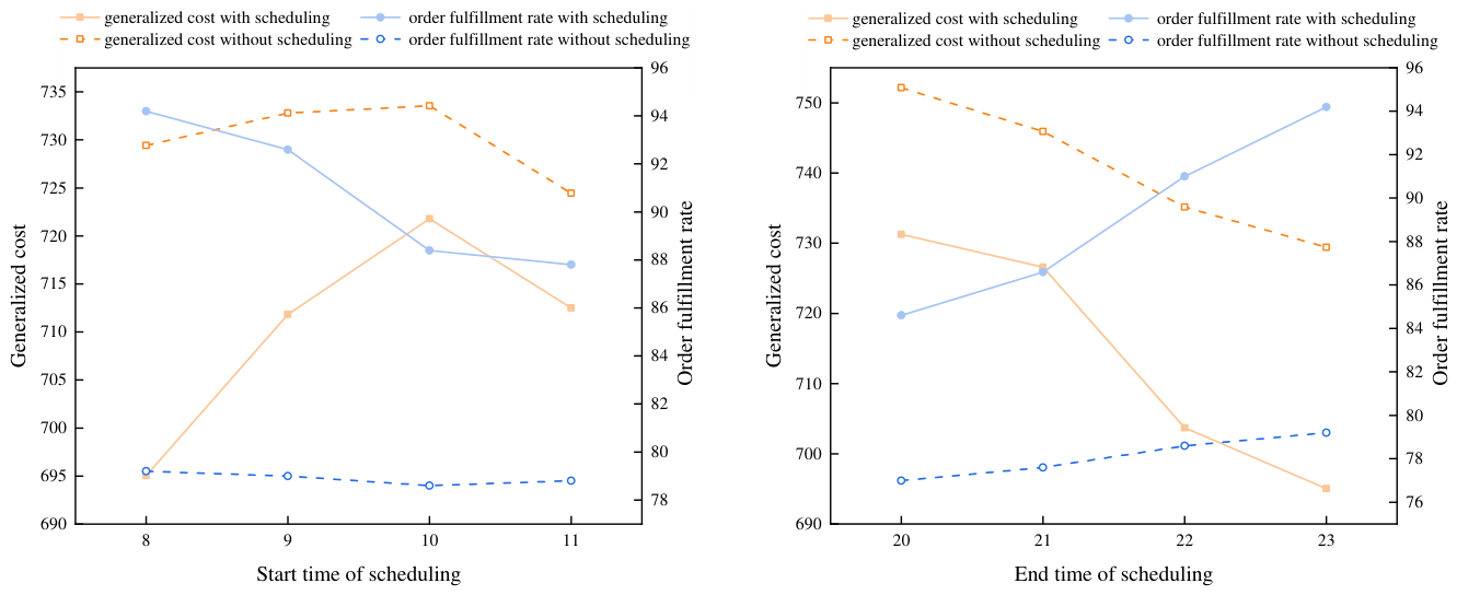
Following these observations, we include additional results for two extra cases in the appendix, as shown in Figure A1 and Figure A2, to examine the robustness of the findings. Overall, these two cases exhibit patterns similar to those in Figure 9. Scheduling substantially improves the fulfillment rate and reduces the generalized cost relative to the no-scheduling baseline. In addition, under the large-demand setting with 500 requests, delaying the start time leads to a more pronounced deterioration in fulfillment performance, whereas extending the end time still tends to deliver better or more stable outcomes.
6.3. Sensitivity Analysis on Fleet Size
We conduct a fleet-size sensitivity analysis for the June 5 case with demand scale 500, where the fleet size is set to 210, 230, 250, 270, and 290 vehicles. Figure 10a illustrates the effects of fleet size on generalized total cost, satisfaction rate, and marginal satisfaction. The formula for marginal satisfaction concerning fleet size is given by Eq. (52). Here, and represent the satisfaction rates under fleet sizes and , with set to 20 in this study. Figure 10b reports the impacts of fleet size on operating cost and the number of relocation tasks. Note that operating cost excludes the fixed cost of vehicles as well as the penalty cost incurred from unmet demand.
Overall, as fleet size increases, the generalized total cost decreases and the satisfaction rate increases. Meanwhile, the marginal improvement in satisfaction is larger at smaller fleet sizes and then gradually tapers off, indicating diminishing returns from further expansion. A notable exception is that the satisfaction rate drops when the fleet size increases from 210 to 230. As shown in Figure 10b, the number of relocation tasks is much higher at a fleet size of 210, suggesting that under tight supply the system may rely on more aggressive relocation and dispatch actions to maintain a relatively high service level; this also leads to higher operating cost and higher generalized total cost. When the fleet size increases to 230, relocation intensity decreases, which may temporarily weaken the correction of station imbalances and result in a short-term decline in satisfaction.
Another important observation is that when the fleet size increases from 270 to 290, the generalized total cost continues to decrease, but the operating cost increases. This implies that the additional reduction in total cost is mainly driven by fewer unmet-demand penalties, while achieving the extra service improvement requires more relocation and dispatch effort. From an operational perspective, moderate fleet expansion is generally beneficial under high demand. However, when the fleet becomes large, expansion decisions should balance service targets against operating costs, so as to avoid introducing excessive operational burdens for limited marginal gains.
6.4. Sensitivity to the Available Vehicle Types
The data from June 1st to June 30th shows the distribution of customer numbers in orders as follows: 87.5% of orders are for 1-2 passengers, 10.75% are for groups of 3-5 people, and 1.75% are for groups of 6-7 people. Consequently, we establish three different types of vehicles to meet customer demands: two-seater economy cars, five-seater comfortable cars, and seven-seater family cars. It is worth noting that the fixed costs and relocation fees for different vehicles are both incremental.
As shown in Figure 11, restricting the available vehicle types can substantially increase the generalized cost. Under all demand scales, using only five-seater vehicles consistently results in the highest generalized cost. Introducing two-seater vehicles to form a mixed fleet leads to a clear cost reduction, and further adding seven-seater vehicles achieves the lowest generalized cost across all demand levels. Table 3 further clarifies the cost composition. Within the generalized cost, the fixed cost accounts for the largest share, followed by the relocation cost , while the penalty cost is relatively small. Compared with VT1, VT2 and VT3 reduce noticeably by incorporating smaller-capacity vehicles. In addition, under medium and high demand, the richer vehicle mix provides better matching for heterogeneous requests, which helps reduce penalties and ineffective relocations caused by supply–demand mismatches. It is also worth noting that, under low demand, the cost difference between VT2 and VT3 is small. As demand increases, the cost advantage of VT3 becomes more pronounced, yielding a lower generalized cost than VT2 and VT1. Overall, vehicle-type configuration has a significant impact on both cost and service performance. However, more vehicle types are not always better. A more appropriate strategy is to select a vehicle mix that aligns with the demand scale and the demand structure, so as to achieve a better balance between cost and service.
7. Conclusions
7.1. Theoretical Implications
This study contributes to the car-sharing scheduling literature in three ways. Firstly, it formalizes an integrated scheduling problem for one-way station-based car-sharing by jointly considering order allocation, vehicle relocation, and dispatcher movement, while allowing a heterogeneous fleet. Secondly, it extends integrated scheduling to a data-driven robust setting by calibrating uncertainty sets from historical observations and accounting for time variability in both dispatcher movement and vehicle relocation, thereby reducing sensitivity to execution-time deviations. Thirdly, it develops a hybrid ALNS/GA solution method with robustness embedded in the search and evaluation, so the integrated robust model remains tractable on realistic instances.
7.2. Practical Implications
The empirical results provide several operational takeaways for station-based car-sharing operators. Integrated scheduling can materially improve both cost and service outcomes compared with non-integrated operations: across the tested cases, it reduces average total cost by about 10.69% and increases order fulfillment by about 16.48%. Building on this, the integrated robust system further reduces cost by 1.96% and improves fulfillment by an additional 0.99%, while producing more stable outcomes across repeated runs. Operators can therefore use integrated scheduling as the default approach, and introduce the robust variant when the system scales up or time-uncertainty risk increases to improve operational reliability. In addition, the sensitivity analyses suggest that fleet size and fleet composition should be adjusted with demand pressure: adding vehicles can reduce generalized cost up to a point, but excessive fleet size may cause station congestion and higher operating burdens; a mixed fleet can be beneficial under sufficiently diverse and large demand, but may increase cost under low demand.
7.3. Limitations and Future Research
This study has several limitations that open clear directions for future work. Firstly, the uncertainty treatment focuses on dispatcher movement time and vehicle relocation time; future work could also incorporate uncertainty in demand volume and cancellations within a unified robust framework. Secondly, the analysis is based on a specific operational setting and dataset; validating the approach across different cities, seasons, and station layouts would strengthen external validity and help calibrate uncertainty sets in practice. Thirdly, the current framework abstracts from several operational features that matter in many platforms, such as dynamic pricing, real-time re-optimization, and electric-vehicle charging constraints. Extending the model to include EV charging and energy feasibility is a natural next step.
Author Contributions
Conceptualization, J.G. and Y.M.; methodology, J.G., Y.D. and M.Y.; software, L.L.; validation, J.G. and L.L.; formal analysis, Y.M.; investigation, J.G., Y.D. and L.L.; resources, J.G. and Y.M.; data curation, Y.D., L.L. and M.Y.; writing—original draft preparation, J.G. and Y.D.; writing—review and editing, Y.D. and L.L.; visualization, Y.M.; supervision, Y.M. and M.Y.; project administration, J.G.,Y.M. and M.Y.; funding acquisition, J.G. and Y.M. All authors have read and agreed to the published version of the manuscript.
Funding
This work was supported by National Natural Science Foundation of China (Grant No. 72202056), Hebei Yanzhao Golden Platform Talent Gathering Program Backbone Talent Project (Grant No. HJYB202532), Supported by Sichuan Science and Technology Program (Grant No. 2025YFNZH0024), and the Program of China Scholarship Council (CSC NO. 202406700017).
Data Availability Statement
The raw data supporting the conclusions of this article will be made available by the authors on request.
Conflicts of Interest
The authors declare no conflicts of interest.
Appendix A
Figure A1.
Start and end times of dispatcher scheduling for Case 6.15-400.
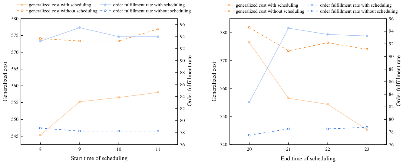
Figure A2.
Start and end times of dispatcher scheduling for Case 6.5-500.
References
- Vega-Gonzalo, M.; Gomez, J.; Christidis, P.; Vassallo, J.M. The role of shared mobility in reducing perceived private car dependency. Transp. Res. Part D. 2024, 126, 104023. [Google Scholar] [CrossRef]
- Mordor Intelligence. Car Sharing Market Size & Share Analysis - Growth Trends & Forecasts (2025–2030). Online report, 2025. Accessed: 2026-01-25.
- Zhang, S.; Sun, H.; Liu, Y.; Lv, Y.; Wu, J.; Feng, X. Carsharing equitable relocation problem: A two-stage stochastic programming approach with learning-embedded endogenous uncertainty in demand. Transp. Res. Part B Methodol. 2024, 179, 102868. [Google Scholar] [CrossRef]
- Kan, H.; Liu, Z.; Zhang, R. Operating policies with temporally and spatially varied parameters in station-based carsharing services. IEEE Trans. Eng. Manag. 2023, 71, 5101–5116. [Google Scholar] [CrossRef]
- Lim, J.; Masoud, N. Dynamic usage allocation and pricing for curb space operation. Transp. Sci. 2024, 58, 1252–1276. [Google Scholar] [CrossRef]
- Guo, J.; Long, J.; Szeto, W.; Tan, W.; Jian, S. Vehicle routing in one-way carsharing service with ridesharing options: A variable neighborhood search algorithm. Transp. Res. Part C Emerg. Technol. 2025, 171, 104983. [Google Scholar] [CrossRef]
- Kayisu, A.K.; Kambale, W.V.; Benarbia, T.; Bokoro, P.N.; Kyamakya, K. A comprehensive literature review on artificial dataset generation for repositioning challenges in shared electric automated and connected mobility. Symmetry 2024, 16, 128. [Google Scholar] [CrossRef]
- Hu, B.; Zhang, Y.; Feng, C.; Dong, X. Understanding the characteristics of car-sharing users and what influences their usage frequency. Inf. Process. Manag. 2023, 60, 103400. [Google Scholar] [CrossRef]
- Liu, X.; Kim, S.W.; Kwon, C. An adaptive large neighborhood search method for rebalancing free-floating electric vehicle sharing systems. Comput. Oper. Res. 2023, 155, 106220. [Google Scholar] [CrossRef]
- Chang, X.; Wu, J.; de Almeida Correia, G.H.; Sun, H.; Feng, Z. A cooperative strategy for optimizing vehicle relocations and staff movements in cities where several carsharing companies operate simultaneously. Transp. Res. Part E Logist. Transp. Rev. 2022, 161, 102711. [Google Scholar] [CrossRef]
- Eilertsen, U.; Falck-Pedersen, O.M.; Henriksen, J.V.; Fagerholt, K.; Pantuso, G. Joint relocation and pricing in electric car-sharing systems. Eur. J. Oper. Res. 2024, 315, 553–566. [Google Scholar] [CrossRef]
- Lu, Z.; Wu, K.; Bai, E.; Li, Z. Optimization of multi-vehicle cold chain logistics distribution paths considering traffic congestion. Symmetry 2025, 17, 89. [Google Scholar] [CrossRef]
- Wang, Z.; Ran, L.; Zhou, M.; He, L. On the equivalence and performance of distributionally robust optimization and robust satisficing models. Manuf. Serv. Oper. Manag. 2025, 27, 1295–1312. [Google Scholar] [CrossRef]
- Basciftci, B.; Koca, E.; Kosunda, S.E. Optimizing strategic and operational decisions of car sharing systems under demand uncertainty and substitution. Comput. Oper. Res. 2025, 180, 107052. [Google Scholar] [CrossRef]
- Rahmanifar, G.; Mohammadi, M.; Golabian, M.; Sherafat, A.; Hajiaghaei-Keshteli, M.; Fusco, G.; Colombaroni, C. Integrated location and routing for cold chain logistics networks with heterogeneous customer demand. J. Ind. Inf. Integr. 2024, 38, 100573. [Google Scholar] [CrossRef]
- Martin, Layla; Minner, Stefan; Marco Pavone, M.S. It’s All in the Mix: Technology choice between driverless and human-driven vehicles in sharing systems. Eur. J. Oper. Res. 2025, 324, 969–980. [Google Scholar] [CrossRef]
- Shui, C.; Chu, J.C.; Shih, C.H. Dynamic relocation problem for free-floating electric carsharing systems with real-time requests. Transp. Res. Part E Logist. Transp. Rev. 2025, 204, 104379. [Google Scholar] [CrossRef]
- Zhang, R.; Kan, H.; Moon, I. Trip pricing in user-based relocation for station-based carsharing systems. IEEE Trans. Intell. Transp. Syst. 2024, 26, 591–603. [Google Scholar] [CrossRef]
- Bruglieri, M.; Pisacane, O. A survey on emergent trends in the optimization of car-sharing systems. Int. Trans. Oper. Res. 2023, 30, 2867–2908. [Google Scholar] [CrossRef]
- Li, M.; Xi, H.; Xie, C.; Shen, Z.J.M.; Hu, Y. Real-time vehicle relocation, personnel dispatch and trip pricing for carsharing systems under supply and demand uncertainties. Transp. Res. Part B Methodol. 2025, 193, 103154. [Google Scholar] [CrossRef]
- Xu, M.; Wu, T. Real-time vehicle relocation and charging optimization for one-way electric carsharing systems. Transp. Res. Part E Logist. Transp. Rev. 2025, 195, 103996. [Google Scholar] [CrossRef]
- Shui, C.; Chu, J.C.; Lin, S.C.; Shih, C.H. Optimization of vehicle charging and dynamic relocation in free-floating electric carsharing systems with advanced reservations. Comput. Ind. Eng. 2024, 190, 110072. [Google Scholar] [CrossRef]
- Yu, Y.; Wang, D.Z.; Tian, Q.; Liu, S. Optimal pricing and hybrid relocation in a free-floating carsharing system with battery swapping electric vehicles. Transp. Res. Part C Emerg. Technol. 2025, 178, 105212. [Google Scholar] [CrossRef]
- Bruck, B.P.; Coutinho, W.P.; Munari, P. The Robust Bike sharing Rebalancing Problem: Formulations and a branch-and-cut algorithm. Eur. J. Oper. Res. 2025, 325, 67–80. [Google Scholar] [CrossRef]
- Wu, T.; Xu, M.; Eltoukhy, A.E. Real-time vehicle relocation and staff rebalancing problem for electric and shared vehicle systems. Int. J. Prod. Res. 2024, 62, 5697–5719. [Google Scholar] [CrossRef]
- Yang, L.; Xu, M.; An, S.; Hu, X. Optimal Dispatcher Number for One-Way Carsharing Services Considering Break Requirement. IEEE Trans. Intell. Transp. Syst. 2024, 25, 5807–5824. [Google Scholar] [CrossRef]
- Tian, T.; Liu, Y.; Yan, B.; Li, J. Vehicle relocation and staff rebalance problem in one-way free-floating car-sharing system: A novel multi-iteration probabilistic greedy algorithm. Expert Syst. With Appl. 2024, 238, 121528. [Google Scholar] [CrossRef]
- Guo, G.; Sun, T. Selective multi-grade charging scheduling and rebalancing for one-way car-sharing systems. IEEE Trans. Intell. Transp. Syst. 2022, 24, 4391–4402. [Google Scholar] [CrossRef]
- Gleditsch, M.D.; Hagen, K.; Andersson, H.; Bakker, S.J.; Fagerholt, K. A column generation heuristic for the dynamic bicycle rebalancing problem. Eur. J. Oper. Res. 2024, 317, 762–775. [Google Scholar] [CrossRef]
- Oliveira, B.B.; Ahipasaoglu, S.D. Enhancing carsharing pricing and operations through integrated choice models. Transp. Res. Part E Logist. Transp. Rev. 2025, 195, 103993. [Google Scholar] [CrossRef]
- Liu, Z.; Raza, H. Data-Driven Two-Stage Distributionally Robust Mean Semi-Variance Mixed-Integer Optimization Model for Location Allocation Problems in an Uncertain Environment. Symmetry 2025, 17, 589. [Google Scholar] [CrossRef]
- Hu, L.; Zhang, Y.; Wen, M.; Leus, R.; Zhang, N. Robust parallel machine selection and scheduling with uncertain release times. Eur. J. Oper. Res. 2025, 327, 838–856. [Google Scholar] [CrossRef]
- Chen, Q.; Ma, S.; Li, H.; Zhu, N.; He, Q.C. Optimizing bike rebalancing strategies in free-floating bike-sharing systems: An enhanced distributionally robust approach. Transp. Res. Part E Logist. Transp. Rev. 2024, 184, 103477. [Google Scholar] [CrossRef]
- Zhang, R.; Xie, C.; Long, D.Z. A data-driven robust optimization model for repositioning problem in bike-sharing systems. Transp. Res. Part E Logist. Transp. Rev. 2025, 201, 104192. [Google Scholar] [CrossRef]
- Castellucci, P.B.; Coelho, L.C.; Darvish, M. A new branch-and-Benders-cut algorithm for the time-dependent vehicle routing problem. Expert Syst. With Appl. 2025, 265, 125996. [Google Scholar] [CrossRef]
- Campos, R.; Coelho, L.C.; Munari, P. New formulations for the robust vehicle routing problem with time windows under demand and travel time uncertainty. OR Spectr. 2025, 47, 411–453. [Google Scholar] [CrossRef]
- Chen, Y.; Liu, Y.; Bai, Y.; Mao, B. Real-time dispatch management of shared autonomous vehicles with on-demand and pre-booked requests. Transp. Res. Part A Policy Pract. 2024, 181, 104021. [Google Scholar] [CrossRef]
- Smet, P. Vehicle substitution in heterogeneous round-trip carsharing systems. Comput. Ind. Eng. 2021, 162, 107703. [Google Scholar] [CrossRef]
- Yang, S.; Wu, J.; Sun, H.; Qu, Y.; Li, T. Double-balanced relocation optimization of one-way car-sharing system with real-time requests. Transp. Res. Part C Emerg. Technol. 2021, 125, 103071. [Google Scholar] [CrossRef]
- Xiong, X.; Li, Y.; Yang, W.; Shen, H. Data-driven robust dual-sourcing inventory management under purchase price and demand uncertainties. Transp. Res. Part E Logist. Transp. Rev. 2022, 160, 102671. [Google Scholar] [CrossRef]
- Bertsimas, D.; Sim, M. The price of robustness. Oper. Res. 2004, 52, 35–53. [Google Scholar] [CrossRef]
- Ma, Y.; Zhang, W.; Feng, C.; Lev, B.; Li, Z. A bi-level multi-objective location-routing model for municipal waste management with obnoxious effects. Waste Manag. 2021, 135, 109–121. [Google Scholar] [CrossRef] [PubMed]
- AbdAllah, A.M.F.; Essam, D.L.; Sarker, R.A. On solving periodic re-optimization dynamic vehicle routing problems. Appl. Soft Comput. 2017, 55, 1–12. [Google Scholar] [CrossRef]
- Ropke, S.; Pisinger, D. An adaptive large neighborhood search heuristic for the pickup and delivery problem with time windows. Transp. Sci. 2006, 40, 455–472. [Google Scholar] [CrossRef]
Figure 1.
Diagram of car-sharing.

Figure 2.
Schematic diagram of the integrated scheduling.
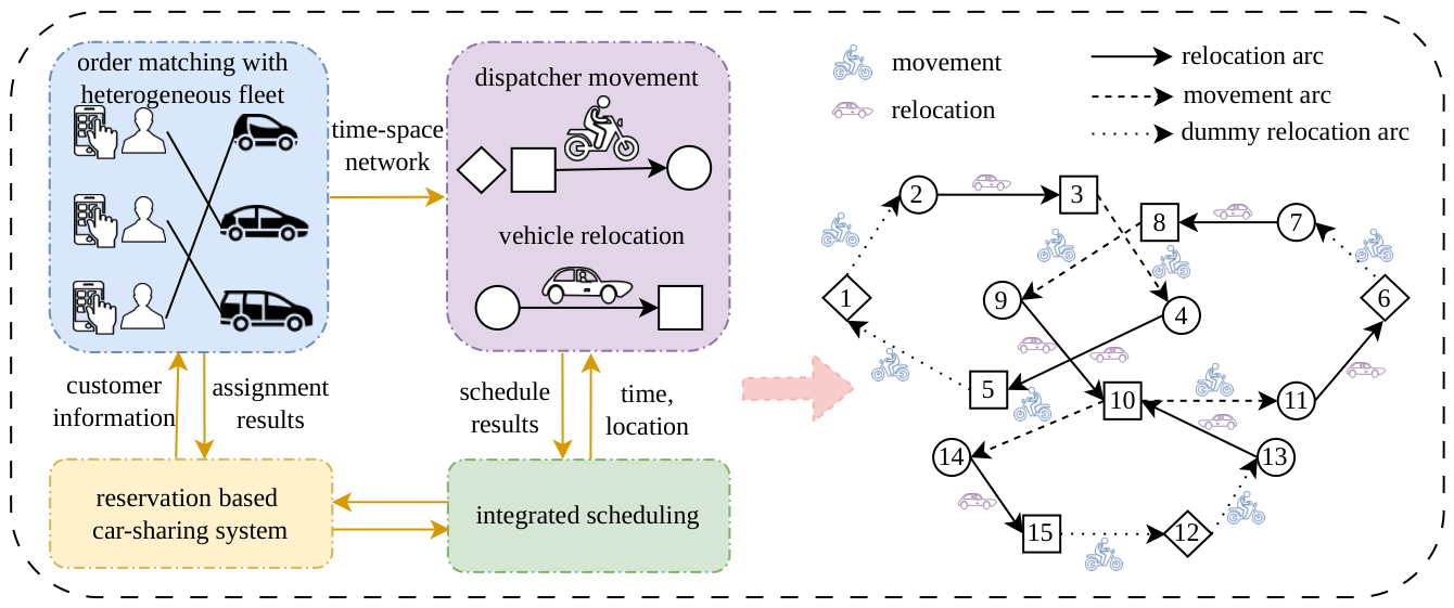
Figure 3.
The routes and scheduling of dispatchers.
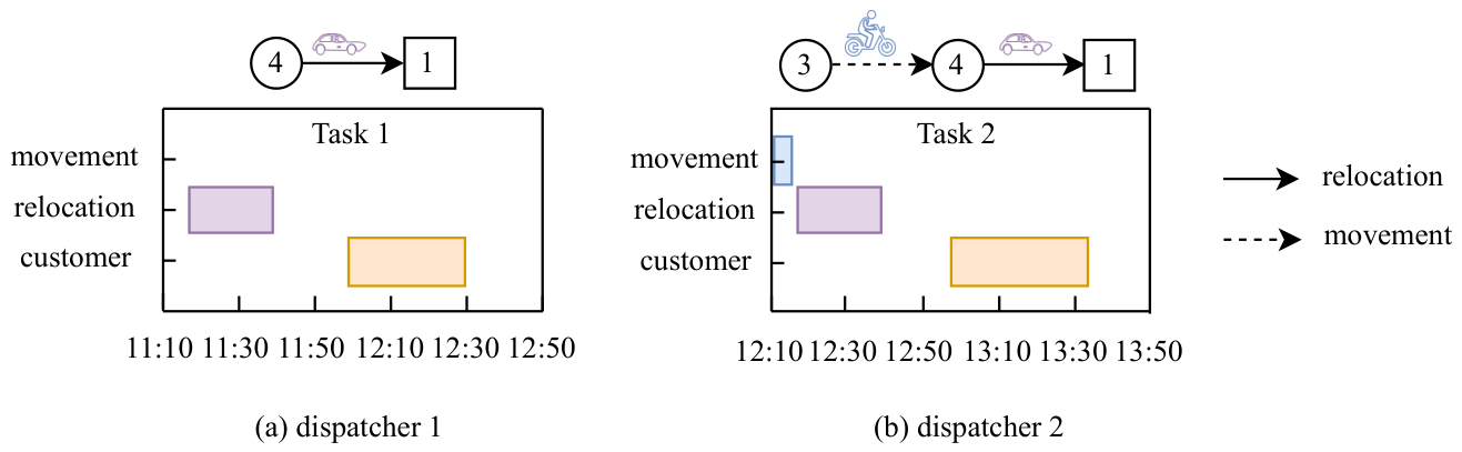
Figure 4.
Stations in Queens.
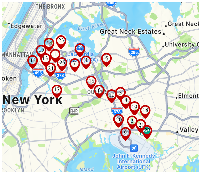
Figure 5.
Comparison of integrated and non-integrated scheduling under different demand levels
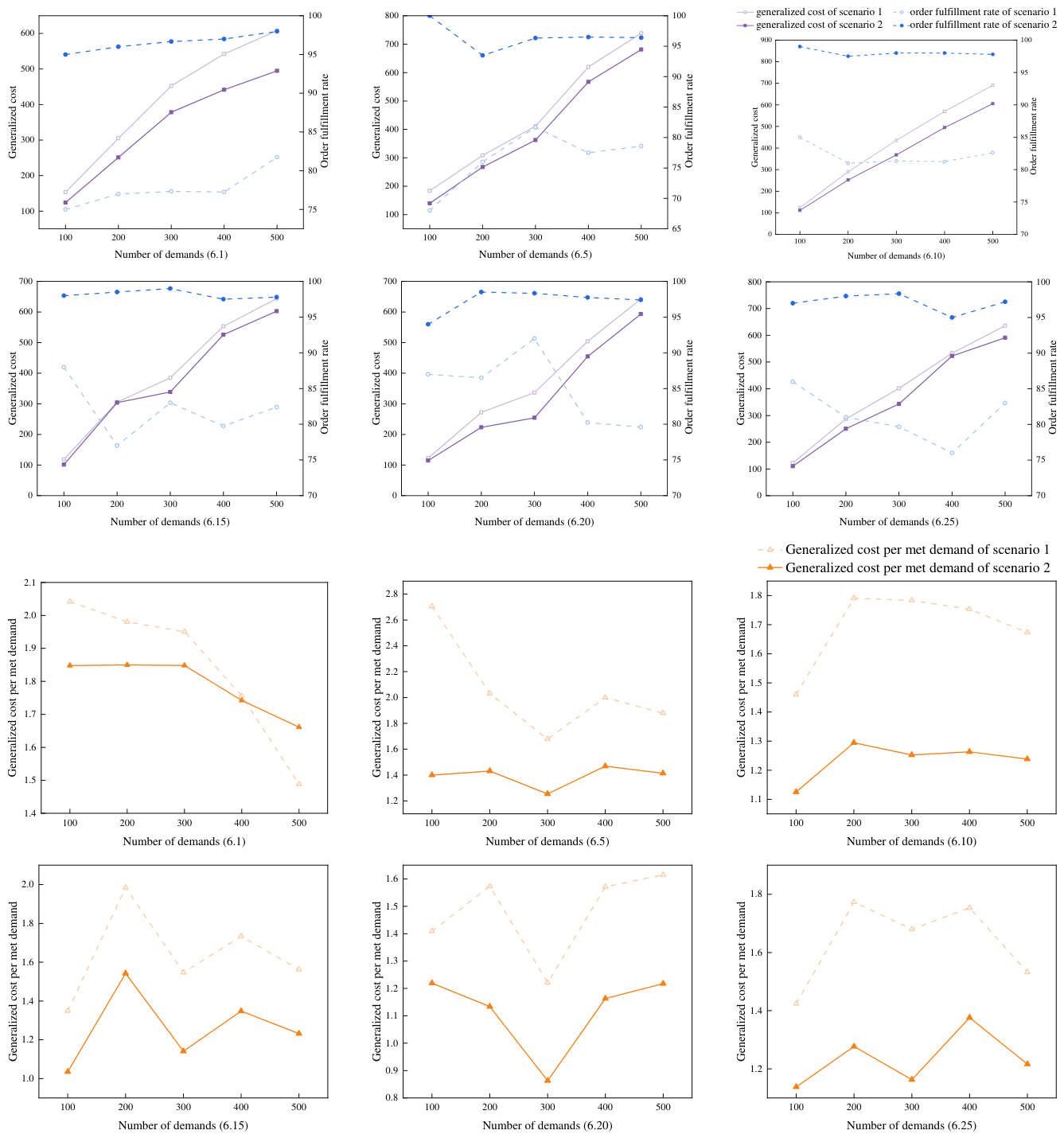
Figure 6.
Generalized costs of Scenarios 2 and 3 over ten independent runs.
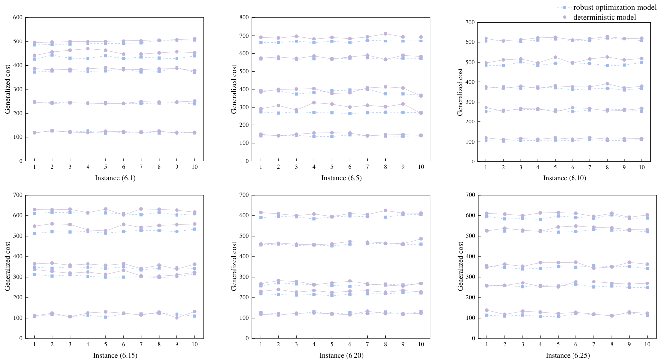
Figure 7.
Temporal distribution of customer demand.
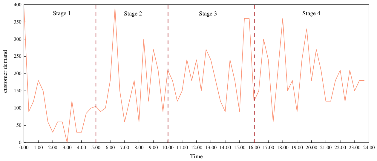
Figure 8.
Aggregate count of vehicles picked up and dropped off at stations.
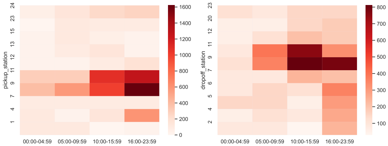
Figure 9.
The start and end times of the dispatcher scheduling.
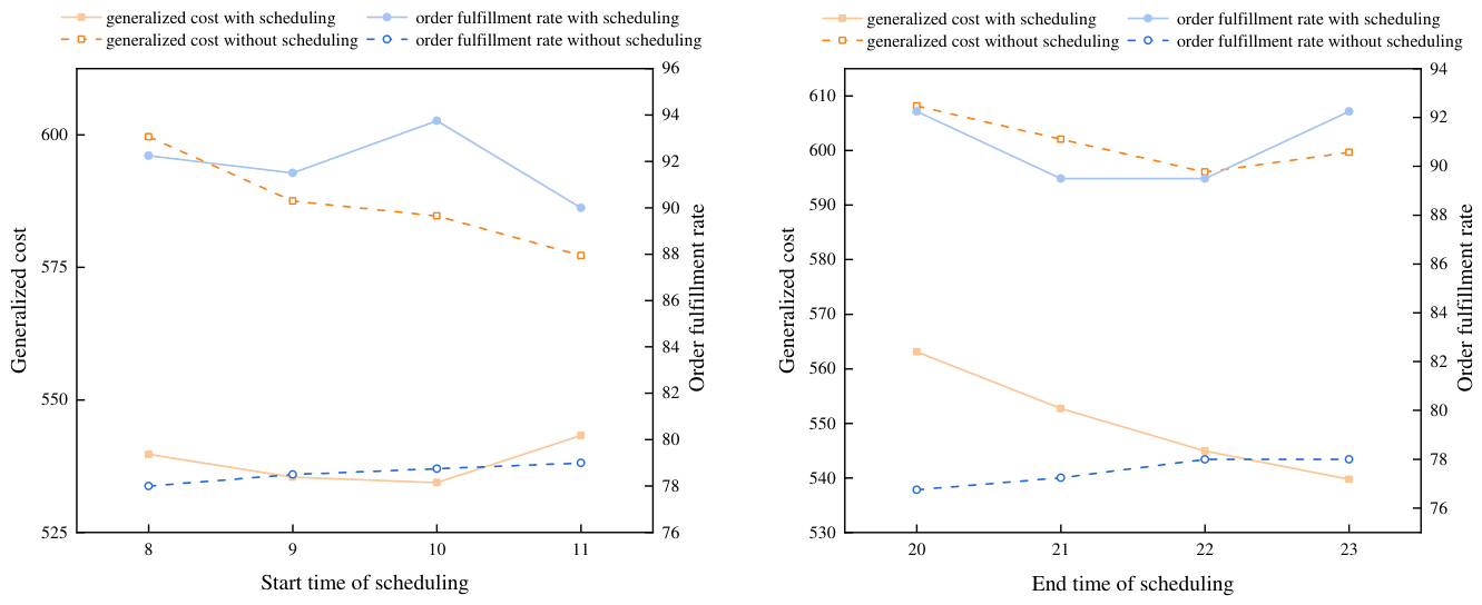
Figure 10.
Performance comparison of different fleet sizes.
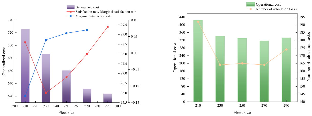
Figure 11.
Performance comparison of different vehicle types under different demands
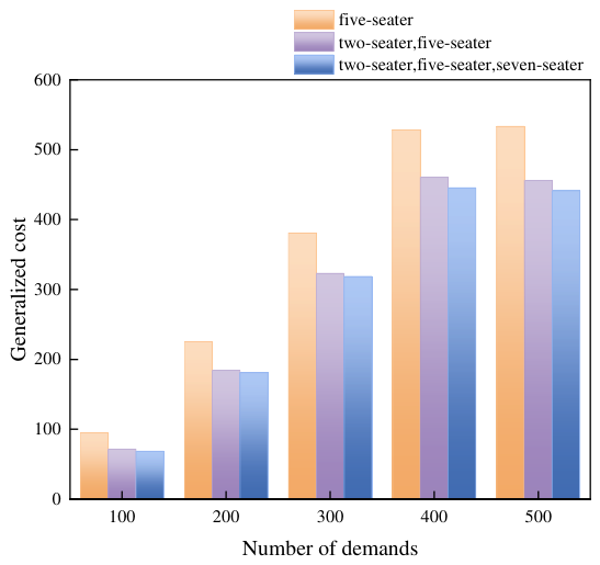

Table 1.
Comparison between the existing literature and this study.
| Reference | Integrated system | Uncertainty | Objective(s) | ||||
|---|---|---|---|---|---|---|---|
| OW | VD | FV | Un | DD | Approach | ||
| Liu et al. [9] | √ | – | Minimize system makespan | ||||
| Zhang et al. [18] | – | Maximize utility | |||||
| Xu et al. [21] | √ | – | Maximize profit | ||||
| Shui et al. [22] | √ | – | Maximize profit | ||||
| Yu et al. [23] | √ | – | Maximize profit | ||||
| Guo et al. [6] | √ | – | Maximize profit | ||||
| Yang et al. [26] | √ | – | Minimize cost | ||||
| Tian et al. [27] | √ | – | Minimize cost | ||||
| Chang et al. [10] | √ | – | Maximize profit | ||||
| Oliveira et al. [30] | √ | – | Maximize contribution margin | ||||
| Guo et al. [28] | √ | √ | – | Minimize response time and operating cost | |||
| Zhang et al. [3] | √ | √ | Stochastic programming | Maximize profit | |||
| Eilertsen et al. [11] | √ | √ | Stochastic programming | Maximize profit | |||
| Bruck et al. [24] | √ | RO with branch-and-cut | Minimize cost | ||||
| Basciftci et al. [14] | √ | √ | Stochastic MIP with branch-and-cut | Maximize profit | |||
| Hu et al. [32] | √ | Two-stage RO with LBBD | Minimize startup cost | ||||
| Smet [38] | √ | √ | Stochastic IP with SAA | Maximize profit | |||
| This study | √ | √ | √ | √ | √ | Data-driven robust optimization | Minimize generalized operating cost |
Note: OW = one-way; VD = integration of vehicle relocation and dispatcher activities; FV = heterogeneous vehicle fleet; Un = uncertain; DD = data-driven.
Table 2.
Results of multi-scenario comparison.
| Case | 100 | 200 | 300 | 400 | 500 | ||||||||||
|---|---|---|---|---|---|---|---|---|---|---|---|---|---|---|---|
| 1 | 2 | 3 | 1 | 2 | 3 | 1 | 2 | 3 | 1 | 2 | 3 | 1 | 2 | 3 | |
| 6.1 | 153.2 | 123.9 | 116.1 | 305.0 | 240.2 | 239.6 | 452.6 | 378.3 | 371.7 | 608.3 | 495.0 | 485.1 | 542.5 | 441.6 | 426.2 |
| 6.2 | 147.0 | 147.2 | 142.9 | 147.4 | 146.5 | 144.9 | 590.0 | 486.0 | 481.5 | 505.3 | 477.1 | 466.4 | 824.4 | 787.3 | 770.4 |
| 6.3 | 130.6 | 120.5 | 119.0 | 247.4 | 212.6 | 204.2 | 411.8 | 386.5 | 384.0 | 504.7 | 466.4 | 465.6 | 622.1 | 597.1 | 584.3 |
| 6.4 | 87.9 | 82.7 | 78.3 | 251.6 | 217.0 | 218.3 | 363.2 | 333.7 | 326.7 | 584.5 | 497.4 | 498.2 | 621.4 | 563.1 | 554.8 |
| 6.5 | 184.0 | 140.0 | 135.9 | 308.8 | 267.6 | 268.0 | 411.2 | 362.3 | 366.9 | 620.0 | 567.1 | 566.5 | 738.4 | 681.4 | 659.5 |
| 6.6 | 96.9 | 92.4 | 85.6 | 218.2 | 195.5 | 193.1 | 299.8 | 262.6 | 264.1 | 341.9 | 319.1 | 318.3 | 449.3 | 408.9 | 393.4 |
| 6.7 | 124.8 | 119.0 | 114.4 | 260.1 | 232.7 | 235.3 | 423.9 | 372.7 | 353.9 | 455.0 | 413.5 | 408.1 | 646.6 | 557.8 | 553.2 |
| 6.8 | 140.7 | 113.2 | 110.0 | 270.8 | 227.7 | 229.3 | 397.8 | 357.0 | 350.8 | 540.6 | 458.0 | 454.5 | 653.3 | 584.5 | 576.8 |
| 6.9 | 148.7 | 115.6 | 111.9 | 321.5 | 275.3 | 280.2 | 413.0 | 358.6 | 341.1 | 530.0 | 500.3 | 497.2 | 704.5 | 626.3 | 604.7 |
| 6.10 | 124.1 | 111.4 | 103.5 | 290.2 | 252.5 | 251.8 | 435.3 | 368.2 | 359.7 | 569.9 | 495.2 | 483.0 | 691.1 | 605.6 | 603.8 |
| 6.11 | 151.1 | 118.5 | 120.0 | 239.2 | 208.2 | 196.3 | 425.3 | 376.7 | 368.2 | 612.1 | 547.8 | 548.2 | 708.0 | 669.1 | 648.3 |
| 6.12 | 95.2 | 85.4 | 89.4 | 218.8 | 199.0 | 201.3 | 357.6 | 330.6 | 318.0 | 452.0 | 417.5 | 415.5 | 575.0 | 537.6 | 528.1 |
| 6.13 | 169.4 | 159.6 | 155.2 | 272.9 | 242.6 | 236.7 | 441.3 | 399.0 | 388.2 | 512.3 | 495.7 | 486.6 | 514.4 | 602.5 | 599.2 |
| 6.14 | 128.0 | 106.5 | 104.0 | 219.4 | 215.5 | 202.6 | 302.6 | 274.9 | 257.8 | 499.2 | 465.4 | 452.6 | 566.5 | 511.9 | 496.7 |
| 6.15 | 118.7 | 101.4 | 104.2 | 305.6 | 303.9 | 297.3 | 385.2 | 338.8 | 334.3 | 553.0 | 525.8 | 512.9 | 643.9 | 602.5 | 602.0 |
| 6.16 | 124.9 | 108.6 | 102.3 | 231.9 | 197.7 | 193.7 | 323.3 | 274.2 | 273.9 | 516.4 | 445.5 | 433.0 | 559.7 | 493.3 | 490.3 |
| 6.17 | 98.0 | 91.1 | 86.9 | 151.3 | 149.2 | 145.5 | 280.8 | 252.3 | 234.0 | 307.8 | 303.8 | 302.9 | 385.5 | 386.6 | 377.3 |
| 6.18 | 119.0 | 101.3 | 104.7 | 257.3 | 234.2 | 235.6 | 436.5 | 377.4 | 377.3 | 564.2 | 488.5 | 472.4 | 646.9 | 589.7 | 576.4 |
| 6.19 | 169.0 | 141.9 | 143.8 | 286.9 | 242.8 | 241.3 | 371.4 | 317.3 | 316.5 | 586.5 | 427.2 | 404.8 | 594.6 | 567.8 | 559.8 |
| 6.20 | 122.6 | 114.7 | 119.1 | 272.1 | 223.4 | 208.1 | 336.9 | 254.6 | 253.3 | 504.3 | 454.7 | 450.5 | 642.7 | 593.0 | 583.0 |
| 6.21 | 130.0 | 109.7 | 105.5 | 253.3 | 228.1 | 223.5 | 410.9 | 342.9 | 337.0 | 592.9 | 485.8 | 474.5 | 552.4 | 496.9 | 494.8 |
| 6.22 | 133.0 | 108.8 | 103.5 | 244.6 | 226.0 | 229.8 | 354.0 | 328.6 | 324.7 | 489.1 | 442.8 | 441.5 | 551.2 | 514.0 | 503.7 |
| 6.23 | 142.6 | 124.7 | 116.6 | 254.1 | 208.9 | 205.7 | 381.3 | 313.6 | 311.0 | 513.9 | 476.1 | 468.8 | 673.6 | 598.8 | 594.8 |
| 6.24 | 136.6 | 121.0 | 123.4 | 279.9 | 250.0 | 247.8 | 417.9 | 360.4 | 349.5 | 534.6 | 499.0 | 474.6 | 675.0 | 616.4 | 613.1 |
| 6.25 | 122.5 | 110.4 | 106.7 | 287.3 | 250.3 | 246.6 | 401.5 | 343.1 | 341.1 | 533.0 | 522.9 | 518.8 | 636.0 | 591.2 | 580.6 |
| 6.26 | 129.1 | 105.3 | 107.4 | 223.8 | 200.1 | 195.5 | 418.6 | 365.6 | 358.1 | 463.2 | 397.6 | 389.0 | 397.6 | 384.9 | 376.1 |
| 6.27 | 130.2 | 112.5 | 107.2 | 158.0 | 152.3 | 135.0 | 414.7 | 386.0 | 378.6 | 491.0 | 490.6 | 479.3 | 543.1 | 496.3 | 494.1 |
| 6.28 | 148.0 | 112.0 | 110.4 | 314.5 | 263.8 | 243.7 | 300.6 | 292.5 | 286.3 | 468.4 | 410.8 | 406.7 | 554.1 | 516.2 | 508.0 |
| 6.29 | 160.1 | 137.5 | 139.2 | 219.2 | 187.2 | 178.8 | 380.9 | 339.3 | 325.4 | 532.3 | 454.0 | 446.8 | 596.0 | 534.1 | 533.5 |
| 6.30 | 140.8 | 118.5 | 106.9 | 234.7 | 229.7 | 224.8 | 405.8 | 395.2 | 385.7 | 552.0 | 517.4 | 504.0 | 678.4 | 615.0 | 603.6 |
Table 3.
Cost analysis of different vehicle types.
| Demand | VT | Generalized cost | FR (%) | ||
| 100 | VT1 | 78.40 | 8.75 | 8.00 | 98.00 |
| VT2 | 52.40 | 11.06 | 8.00 | 98.00 | |
| VT3 | 54.83 | 13.71 | 0.00 | 100.00 | |
| 200 | VT1 | 156.80 | 52.41 | 16.00 | 98.00 |
| VT2 | 106.20 | 62.06 | 16.00 | 98.00 | |
| VT3 | 110.93 | 61.93 | 8.00 | 99.00 | |
| 300 | VT1 | 233.60 | 115.05 | 32.00 | 97.33 |
| VT2 | 157.17 | 127.18 | 38.67 | 96.78 | |
| VT3 | 162.83 | 129.26 | 26.67 | 97.78 | |
| 400 | VT1 | 310.40 | 169.96 | 48.00 | 97.00 |
| VT2 | 213.03 | 198.17 | 49.33 | 96.92 | |
| VT3 | 220.07 | 192.06 | 33.33 | 97.92 | |
| 500 | VT1 | 310.40 | 175.19 | 48.00 | 97.00 |
| VT2 | 214.27 | 190.99 | 50.67 | 96.83 | |
| VT3 | 221.07 | 182.93 | 37.33 | 97.67 | |
Note: VT1: five-seater; VT2: two-seater and five-seater; VT3: two-seater, five-seater, and seven-seater.
Disclaimer/Publisher’s Note: The statements, opinions and data contained in all publications are solely those of the individual author(s) and contributor(s) and not of MDPI and/or the editor(s). MDPI and/or the editor(s) disclaim responsibility for any injury to people or property resulting from any ideas, methods, instructions or products referred to in the content. |
© 2026 by the authors. Licensee MDPI, Basel, Switzerland. This article is an open access article distributed under the terms and conditions of the Creative Commons Attribution (CC BY) license (http://creativecommons.org/licenses/by/4.0/).
Copyright: This open access article is published under a Creative Commons CC BY 4.0 license, which permit the free download, distribution, and reuse, provided that the author and preprint are cited in any reuse.