

Submitted:
14 September 2026
Posted:
15 September 2026
You are already at the latest version
Abstract
Building on the published finite-resolution, background-independent framework for local semiclassical gravity, this work examines its phenomenological consequences across cosmology and particle physics. The underlying construction is formulated on a causal diamond equipped with a boundary-completed algebra, reflecting the non-factorization of the diffeomorphism-invariant Hilbert space. This algebra supplies the edge data needed for a local Wheeler--DeWitt description and is shared by the operational state and semiclassical reference family, whose relative entropy defines the local response. The entropic boundary capacity, with its topological term set by the Euler curvature charge, fixes an effective channel multiplicity \( N\approx1.23\times10^{11} \). Calibrating the coherent tensor response to Newton's constant then gives the matching scale \( M_s\approx3.02\times10^{13}\,{\rm GeV} \). In the equilibrium KMS regime, the leading relative-entropy Hessian separates into tensor, vector, and scalar response blocks, which a quasi-local heat-kernel expansion connects to the effective theory at the matching scale. The finite--continuum bridge uses the noncommutative-geometric algebra \( \mathcal A_F\simeq\mathbb C\oplus\mathbb H\oplus M_3(\mathbb C) \) with a common trace convention to map finite responses to Standard-Model observables. Once the boundary capacity, Newton calibration, and finite internal structure are fixed, the primary projections require no sector-specific continuous retuning. In cosmology, finite-resolution saturation identifies the scalaron pole with the matching scale, \( M_R=M_s \), and fixes the curvature stiffness \( \lambda_{R^2}=N_{\rm eff}/12 \). The isotropic boundary response gives the coherence duration \( \mathcal N_*=18\pi \), yielding \( n_s\approx0.9646\ \)and \( r\approx0.0038 \). All continuous dimensional scales cancel from the primordial scalar amplitude, leaving the finite-capacity relation \( A_s=81\pi/N \). Extensions of the same response give exploratory late-time targets for vacuum energy, structure growth, and the acceleration scale. In particle physics, single-pixel scalar saturation provides linked electroweak consistency tests, while the vector Hessian fixes correlated gauge responses. At the matching scale the construction gives \( \alpha_s^{-1}=12\pi, \alpha_{\rm em}^{-1}=36\pi \), and \( \sin^2\theta_W=7/18 \). The same finite geometry carries a Lie-theoretical filtration \( G\to\mathfrak g\to T \), whose successive accessibility levels organize the charged-lepton mass hierarchy, while canonical anticommutation relations provide the fermionic operator structure supporting the quark Yukawa hierarchy. Finally, finite-mesh simulations test the main analytical mechanisms numerically across the boundary, cosmological, gauge, and flavor sectors, including the modular filtration that selects the threefold generation carrier. The resulting cross-sector consistency makes the construction constrained and fragile in a useful sense: changing a shared input affects several sectors at once.
Keywords:
quantum gravity
; semiclassical gravity
; entropic gravity
; relative entropy
; causal diamonds
; finite-resolution boundaries
; boundary-completed algebras
; Wheeler–DeWitt equation
; modular flow
; Kubo–Mori metric
1. Introduction
A finite-resolution, background-independent framework for local semiclassical gravity was recently developed [1]. That work established an axiomatic causal-diamond architecture equipped with a relative-entropy variational principle and open-modular dynamics.
The published framework identified linked phenomenological targets across cosmology and particle physics, including a quantum-gravitational account of accelerated expansion. The present paper develops and audits these consequences across physical sectors. We take the causal-diamond algebra, topology-locked capacity, Newton-calibrated matching scale, relative-entropy Hessian, and open-modular dynamics from [1], recalling only what is needed here. We then make the finite–continuum bridge explicit and connect the finite response architecture to cosmological and Standard-Model observables.
The axioms determine the dimensionless capacity and coherence data , after which Newton’s constant enters once to set the physical matching scale . At the matched equilibrium reference state, the Kubo–Mori relative-entropy Hessian decomposes into orthogonal tensor, vector, and scalar response blocks. Its spectral representation yields the matching-scale Lagrangian. The CPTP dynamics, Lie filtration, and Walsh filtration determine the update rule, mass-response accessibilities, and generation carrier, respectively. Schematically,
In a discrete architecture, an explicit finite–continuum bridge is essential for turning microscopic dynamics into calculable continuum physics. The bridge draws on the internal algebra established in noncommutative-geometric formulations of the Standard Model and fixes a common trace convention.
Because these sectors share the same architecture and trace normalization, their constraints remain structurally linked across otherwise distinct physical responses. This shared origin turns phenomenology into a direct cosmoparticle consistency audit. Once the Newton calibration, finite boundary capacity, and internal algebra are fixed, the framework must recover the cosmological, gauge, electroweak, and mass-sector targets without new phenomenological scales. This makes the construction usefully rigid and falsifiable.
The paper is organized as follows. To keep the audit reasonably self-contained, Section 2 and Section 3 briefly recall the essential structures developed in the foundation paper [1]. Section 4 provides the finite–continuum bridge and common trace convention required for the phenomenological audit. Section 5 derives the macroscopic tensor projection and cosmological targets, while Section 6 develops the cosmoparticle sector (electroweak, gauge, charged-lepton, and quark responses). Section 7 audits their cross-sector consistency, rigidity, and failure modes. Section 8 summarizes the architecture and cross-sector audit, then outlines the remaining open problems.
2. Conceptual Foundations
This section recalls the minimal boundary architecture developed in [1] as needed for the phenomenological audit. The goal is not to repeat the full axiomatic variational derivation, but to specify the fixed structures that enter the sectoral constraints.
The finite-resolution framework for defining local quantum subsystems in semiclassical gravity is organized around the Wheeler–DeWitt (WDW) constraint [2]:
where the global state is constrained rather than time-evolved, and the operator encodes gravitational constraints and diffeomorphism invariance.
To ensure background independence, we treat dynamics as local statistical inference on causal diamonds , the fundamental units of accessible correlations [3]. Because the diffeomorphism-invariant physical Hilbert space does not factorize, each causal diamond is equipped with boundary completion that stores the edge data required for a subregion [4,5]. In the small-diamond regime, modular flow supplies the intrinsic local clock [6,7].
The local semiclassical fields are inferred from the relative-entropy mismatch between the actual boundary-completed state and the corresponding reference family [8,9,10,11]. For each member, the mismatch measures the information cost of accounting for the fixed boundary record with the corresponding candidate field configuration.
2.1. Axiomatic Basis: Minimal Architecture
In a background-independent theory, there is no external stage for local observables [3]; locality must therefore be defined operationally from finite records. The causal diamond, generated by two timelike-separated events (spatial topology ), provides the minimal covariant laboratory for this inference [4]. Within this finite region, diffeomorphism and Gauss-law constraints prevent the interior from forming an autonomous quantum subsystem. A local algebra must therefore include explicit boundary charges, fluxes, and edge data [5,12,13].
Gluing the two spatial halves across their common waist gives a topological , while modular flow provides the intrinsic clock. Together, they define the compact history manifold . Finite resolution then allows the boundary state and semiclassical reference family to be compared by relative entropy, without introducing a preferred lattice or external field content.
The boundary architecture fixes the intrinsic capacity N, while Newton calibration sets the matching scale .
The axioms below (P1–P7) isolate the minimal ingredients required to construct this algebraic arena. Topology, transport, and spin structure specify the minimal boundary sector, while constitutive relations calibrate its microscopic capacity to macroscopic gravity.
Principle A: Operational Locality and Boundary Completion
P1 (Non-factorization). The diffeomorphism-invariant physical Hilbert space does not factorize across spatial subregions (). Constraint relations tie interior data to boundary charges and fluxes, requiring explicit boundary data (edge modes) to ensure algebraic consistency between adjacent subregions [5,13,14,15].
P2 (Causal Diamonds). A finite experiment is a closed query–response loop between two timelike-separated events p and q. A causal diamond [4] covariantly defines an observer’s operational workspace. We restrict to the minimal simply connected sector: a maximal spatial slice of topology with a single closed waist . This is the minimal local topology supporting a closed boundary completion (P3); nontrivial topologies require extra gluing data and lie outside the present analysis.
P3 (Boundary Completion). Since the physical Hilbert space does not factorize (P1), a well-defined subregion algebra requires boundary completion. States are positive, normalised functionals on . This interface acts as a coherency screen at the diamond waist , reconciling overlapping past and future boundary data into a unified record. We adopt a boundary-completed algebra whose finite-resolution centre carries the gluing and charge labels needed to encode Gauss-law constraints. This ensures that and live on identical operator content and define a common variational domain [5,12,13].
Principle B: Finite Modular Resolution
P4 (Modular Locality). In the local Rindler regime, the vacuum restricted to the boundary-completed algebra is approximately KMS with respect to geometric modular flow. This applies to small causal diamonds whose size lies between the finite-resolution scale and the local curvature radius. In this intermediate regime, the modular Hamiltonian is well approximated by the local boost generator, fixing the KMS period to (compact modular cycle) [6,7].
Corollary (Canonical History Manifold). In the minimal simply connected sector, the two halves glue across the waist to form , while the KMS condition supplies a compact modular cycle , giving the minimal spectral history manifold .
P5 (Finite Resolution). Defining a local subsystem requires finite resolution to ensure a stable restriction to and a bounded mode density at the interface. Since an algebraic restriction alone cannot fix the physical bandwidth, a proper-distance cutoff is introduced via a stretched screen in the local Rindler region. This regulator makes the comparison of and operationally finite at the resolved scale, consistent with holographic bounds, giving each resolved superselection sector a finite statistical capacity [16,17,18]. For a scale-free closed screen, topological capacity is its intrinsic topological charge [19,20]; in two dimensions, this is the Euler curvature charge [21].
Corollary (Monotone Spectral Suppression). Relative entropy is monotone under the restriction of the accessible algebra (P3), while finite resolution imposes a strict limit on the information capacity per pixel (P5). In the resolved quasi-local regime, the infrared expansion is therefore organized in terms of intensive response densities and irrelevant corrections suppressed by powers of . Extensive macroscopic quantities may grow with the total number of pixels, but the distinguishability available to each pixel remains bounded by the finite-capacity algebra.
Principle C: Quantized Boundary Sectors and Isotropic Transport
P6 (Gauge Topology). Boundary charge sectors are encoded by topological current data compatible with non-factorization (P1) and closed algebraic gluing (P3). During one modular cycle, the causal-diamond waist sweeps out the closed boundary history , whose current response is represented by a Chern–Simons functional [22]. With the trace normalization fixed, large gauge transformations of compact simple groups shift this functional by integer multiples of ; path-integral phase invariance therefore requires [23]. Gauss law makes interior flux end on the spatial interface as representation-carrying punctures. These punctures generate surface states described by Wess–Zumino–Witten conformal blocks, equivalently chiral data organized by the affine Kac–Moody algebra at level k [24]. Retaining sectors compatible with KMS periodicity, large-gauge invariance, and anomaly inflow, this integer level fixes the normalization of the pure boundary-current response. The full gauge stiffness then follows from the finite trace over the internal inventory, naturally incorporating its specific representation weights.
P7 (Discrete Isotropic Transport). A finite-resolution architecture requires a local transport layer that is inversion-symmetric, isotropic after modular averaging, minimal among sets spanning three spatial directions, and compatible with spinorial matter. Inversion symmetry pairs every direction with its opposite, so minimal spanning transport consists of three antipodal unit-axis pairs. Equal-weight isotropy forces these axes to form an orthonormal triad, . Up to rotation and relabeling, the unique minimal router is therefore the signed octahedral set , with coordination and the associated step rule. Modular closure requires a transport cycle to return local excitations to the same physical state, up to spinorial sign. Supporting local spinors therefore lifts to its double cover and introduces the corresponding spin-parity grading.
Corollary (Resolved Modular Interval and Lorentz Covariance). The cutoff is placed at fixed proper distance from the causal-diamond waist. Because the background-independent diamond is defined by light rays, this local placement introduces no preferred global frame. Under local Rindler scaling , identifying the minimum resolved proper time with fixes the canonical modular threshold . Excising the unresolved neighborhoods of the modular tips then restricts the flow to , with the discrete transport layer confined to the boundary completion near these endpoints. Below , the resolved interior is described by continuum fields on a smooth manifold; this effective description is locally Lorentz invariant, with regulator artifacts appearing only through irrelevant operators suppressed by powers of .
Corollary (Tip Defect Parameter ). Routing continuous modular flow through the sub-resolution tips p and q creates an irreducible digitization cost. By P7, local isotropy fixes the mean-square transfer fraction along any resolved direction to . Four equilateral triangles meet at each of the six octahedral vertices, leaving a local Regge deficit of . The octahedral mesh therefore reproduces the isotropic fraction through both its normalized coordination deficit and its normalized Regge deficit . Normalizing the transfer fraction over the Euclidean modular cycle (P4) gives . Because p and q are the two endpoints of a single source-to-sink causal transfer, this index enters the static boundary capacity once.
Corollary (Transport-Orientation Redundancy ). The octahedral router contains three antipodal axis pairs, . Independent reversal of each orientation label generates , hence .
Corollary (Pixel). At finite resolution, a pixel represents a single resolvable algebraic patch on the boundary, defined by the triple and represented by a node in the mesh. The local algebra acts on the internal fiber , while the transport operator D provides the nearest-neighbor connectivity routing data between adjacent nodes.
The axioms operate hierarchically. P1–P3 define the subsystem: a causal diamond completed by boundary data on a closed waist. P4–P5 supply the intrinsic modular clock and finite physical bandwidth. P6–P7 provide the quantized currents and isotropic transport required for gauge and spinorial data. Operationally, the diamond is the container, boundary completion the interface, modular flow the clock, and the signed octahedral rule the router. Together, these define the selected boundary sector and the invariant data entering the capacity prescriptions below.
2.2. Intrinsic Boundary Capacity and Effective Channel Multiplicity (N)
In a background-independent, scale-free setting, topology provides an intrinsic carrier of information: when size and shape are removed, information can remain encoded in global structure, as illustrated by topological quantum memories and topological entanglement entropy [20,25,26]. This idea has a long tradition across information theory, quantum matter, topology, and operator algebras [19,27,28,29,30]. Gravity also provides a direct precedent: black-hole entropy is a horizon Noether charge [31,32]. We therefore identify logarithmic topological capacity with the Euler curvature charge , a metric-independent local curvature invariant of a closed surface [21,33].
Finite resolution gives the causal-diamond boundary a finite logarithmic capacity. In the selected sector, this capacity has three irreducible scale-free contributions: Euler charge of the closed waist, modular tip defect, and spin-parity twist.
Boundary completion requires a topologically closed interface for the Gauss-law encoding of interior charge. On the simply connected waist , the available additive, scale-free local curvature invariant is the Euler term, consistent with Hadwiger’s characterization of additive valuations [34]. With the scalar-curvature convention , Gauss–Bonnet gives rather than the Gaussian-curvature value [35,36]:
This is a global topological capacity, not an extensive thermodynamic entropy: the waist radius cancels and only the Euler class remains. The contribution is therefore counted once for the complete gluing surface, rather than independently for each resolved pixel.
At the diamond tips , the transverse cross-section falls below the resolution length (P5). Smooth modular flow can no longer be represented as a continuous transverse field and must pass through the discrete transport layer of P7. Local isotropy gives the spatial routing fraction , while one resolved modular interval contributes of the Euclidean modular circle, giving:
Thus measures the finite-resolution bottleneck associated with routing smooth modular flow through the unresolved endpoints. Because p and q are the endpoints of a single source-to-sink causal transfer, this bottleneck enters the logarithmic capacity additively exactly once.
The discrete transport structure (P7) must support local spinors, requiring the lift . This induces a nontrivial spin-parity grading that separates bosonic and fermionic transport around closed modular loops. In each fixed central and gauge sector, the corresponding parity fixed-point inclusion has index two [37], hence statistical dimension and .
The intrinsic capacity of the resolved boundary sector is therefore:
With we obtain:
As an exponentiated capacity rather than a microscopic Hilbert-space dimension, N need not be an integer.
This result is also computationally corroborated by the simulations of [38] through successive finite-mesh refinements.
This establishes the intrinsic, scale-independent entropic capacity of the finite-resolution causal diamond.
2.3. Coherent Participation and Matching Scale
The channel multiplicity N represents the boundary capacity, while is the part that participates coherently in the tensor response. In the open-modular fluctuation–dissipation closure of Section 3, the coherent fraction is identified with . To quantify it, we introduce an operator (), whose eigenvalues measure the phase survival of each channel over one modular cycle. Its normalized trace gives:
Here, Tr is an effective trace over the boundary capacity, with giving the total weight and the coherently participating part.
Intuitively, these coherent channels act like springs in parallel. Taking each to contribute a stiffness of order yields the macroscopic constitutive relation [39,40,41]:
This hierarchy mirrors Dvali species-bound scaling [41]. While sets the operational finite-resolution scale, measures the collective tensor stiffness of the boundary. The Planck scale is therefore not the microscopic regulator of an continuum limit, but a macroscopic consequence of coherent channel multiplicity.
This calibration is strictly non-circular: the boundary architecture and capacity prescription fix N, while the coherence closure fixes , both entirely independently of the observed value of G, which then determines .
We now calibrate the resolution scale against Newton’s constant G using the reduced Planck mass to align with the standard Einstein–Hilbert action. This calibration does not predict Newton’s constant; it uses the observed value of G to assign the matching scale after has been fixed by the boundary sector. The constitutive relation then gives:
Physically, represents the resolution limit of the algebra (sharp focus) where the EFT problem is well-posed: at this scale, gravitational stiffness, gauge couplings, and mass gaps enter as unified matching data, with some quantized-sector conditions reducing to closed-form constraints.
2.4. Fixed Architectural Ingredients
Table 1 summarizes the fixed minimal-sector architectural ingredients used in the present audit. The origin column identifies their published basis in [1], while the final column records their downstream roles. Its ordering makes the logical chain from the axioms to the physical matching scale explicit.
3. Relative-Entropy Hessian and Open-Modular Dynamics
This section recalls the relative-entropy Hessian and open-modular dynamics published in [1] as needed for the phenomenological audit. Full derivations and formal extensions are given in the original article.
Dynamics on a causal diamond emerge not as the time evolution of a global Wheeler–DeWitt state [2], but as local statistical inference. Because local AQFT algebras are Type III, ordinary density matrices and traces are unavailable. Finite resolution replaces the sharp local algebra with the boundary-completed effective algebra , providing a common domain with a faithful KMS reference state [42,43]. On this domain, supplies the operational data, while geometry and background fields enter through the semiclassical reference family . The resolved algebra fixes which physical distinctions the causal diamond can register.
The framework anchors the subsystem at finite resolution on a boundary-completed algebra, transforming the variational problem into a matching-scale effective theory at [44]. The local dynamics are organized by the relative entropic mismatch functional at fixed [43,45,46]. Relative entropy therefore measures the information cost of explaining the fixed boundary data with a deformed background . Around a matched reference point, its Hessian naturally decouples into independent tensor, vector and scalar blocks, making a joint matching of all three sectors well-posed.
3.1. Relative-Entropy Functional and Operational Domain
We fix the container with proper-distance regulator (), varying only the reference family on the fixed algebra . The diamond endpoints, algebra, and physical regulator are not varied; all sectors are evaluated on the same finite operator domain. We define the variational functional [46]:
3.2. Hessian Decoupling
Local background fields (metric , gauge field , scalar ) couple on the boundary algebra to three composite operators: the stress tensor , the conserved current , and the scalar density M. To fix normalizations unambiguously, the source–operator pairing is
where the factor is the usual metric-source convention.
At equilibrium, , so and the first variation vanish by the local entanglement first law. The boundary algebra resists informational deformations like a spring displaced from equilibrium. The leading response is therefore quadratic and governed by the Hessian kernel:
For centered tangent modular deformations, this evaluates to the Kubo–Mori inner product [46,48,49]:
The quadratic contribution to I is thus , and the Hessian is the local stiffness matrix of distinguishability [50].
Within the finite-resolution boundary-completed algebra , modular flow is generated by the geometric boost (P4), fixed by the causal diamond and its waist. The source-label symmetries preserved by the boundary architecture commute with the reference modular flow, [5,51]. Metric, gauge-connection and scalar deformations therefore transform as inequivalent source modules. Schur’s lemma and Ward identities forbid symmetry-preserving maps between these modules, giving for in the leading quadratic response.
Because modular flow acts as a geometric boost (P4) and transport-layer anisotropy averages to zero over a full orbit, the reference vacuum is isotropic and parity-even. Local deformations therefore decompose into orthogonal spin channels (transverse-traceless tensors, conserved vectors, scalars), with the grading (P7) isolating the fermionic sector. By symmetry, Kubo–Mori cross-pairings between these representations vanish:
At the symmetric matched KMS reference, the Hessian therefore block-diagonalizes for the leading quadratic Kubo–Mori response. This is tangent-space decoupling, not dynamical isolation: while mixed terms vanish under projection, nonlinear or mixed interactions can reappear at higher variations.
The supplementary script hessiansectordecoupling.py tests this separation on an octahedrally refined boundary [38]. Starting from a generic dense local-fiber Hessian with tensor, vector, and scalar mixing, it applies the finite octahedral Reynolds projection. Figure 1 shows the resulting trace-free response blocks.
3.3. Spectral Factorization and Matching-Scale Action
For slowly varying sources, the finite modular structure is not resolved at leading order, and noncommutativity with the modular background is suppressed. In this regime, the discrete transport admits a continuum description through the covariant operator , giving the Kubo–Mori Hessian a leading quasi-local spectral representation:
The same finite resolution that defines the stretched horizon also sets the physical EFT cutoff (Nyquist frequency). Deformations with physical momentum are unresolved and integrated out of the effective description (effectively aliased away). Evaluated on the history manifold, the heat-kernel trace extracts the local EFT coefficients. Operationally, the heat kernel counts the resolved modes available to carry each response and packages them into local EFT coefficients.
For slowly varying sources, quasi-locality factorizes the trace into three ingredients: an effective four-volume, the internal channel multiplicity, and the bandwidth scale. Absorbing the universal density-of-states factors yields [52,53]:
This acts as the finite-resolution analogue of Weyl’s law. The spectral trace counts the total response modes resolved by the finite boundary algebra. Dividing it by the internal capacity N and the bandwidth density strips away sub-resolution details, leaving only the coarse-grained four-volume seen by the infrared EFT. Volume is therefore read from the resolved spectral count, not assumed as a primitive continuum measure.
This spectral–volume factorization generates the macroscopic scale hierarchy. The tensor sector samples the coherent subset , making Einstein stiffness extensive in channel number. By contrast, vector and scalar responses are normalized per channel, so and the mass susceptibilities remain intensive at .
The spectral trace over the minimal compact operational history then establishes a spectral–volume correspondence. In the small-diamond/KMS regime, modular time forms a thermal circle [6,42]. Identifying the spatial part as two halves glued across the waist (), the minimal manifold for the trace is [52].
Tensor response. The operators derived above govern the low-curvature regime. The Einstein term contains no intrinsic saturation scale. As approaches , finite boundary resolution supplies the first saturation correction to Einstein stiffness, marking the two-derivative operational limit.
We therefore restrict the completion to the homogeneous and isotropic scalar-curvature sector. In this reduced projection, is the only retained local four-derivative invariant: the Gauss–Bonnet density is topological, while anisotropic curvature structures lie outside the projection. The term therefore constitutes this leading local completion.
In four-dimensional Einstein-normalized gravity, this mode is the scalaron. Taking the trace of the vacuum field equations, its pole satisfies [54,55]
Operationally, is the compliance length of Einstein stiffness. While a generic EFT may introduce an independent scale for each higher-curvature correction, the selected finite-resolution sector has only one physical bandwidth. The minimal one-resolution saturation condition therefore sets . This yields
This reproduces the coefficient obtained by the spectral matching in [1], now expressed through the scalaron condition. The same pole relation follows from the scalar–tensor representation. The factor is the universal four-dimensional scalaron normalization of Einstein-normalized gravity; the framework-specific input is the one-resolution condition .
This exact pole relation follows equivalently from the scalar–tensor representation. The factor is the universal four-dimensional scalaron normalization of the Einstein-normalized theory; the framework-specific input is the one-resolution matching .
The boundary bandwidth therefore does more than regulate the theory: it fixes the onset of its leading scalar-curvature completion. The reduced high-curvature response enters the Starobinsky plateau universality class without introducing a second curvature scale. In this sense, the Starobinsky regime is the elastic limit of the finite-resolution vacuum, reached when Einstein stiffness begins to saturate at .
Below , this relation serves as the matching-scale boundary condition for the reduced scalar-curvature sector. Standard running and threshold effects govern the retained couplings, while Wilsonian decoupling suppresses additional higher-dimensional finite-resolution operators by powers of . Within the selected one-resolution sector, no independent curvature scale or continuous matching parameter is introduced.
Vector response. For a compact current algebra with fixed generator and charge normalization, quantum consistency under large gauge transformations quantizes the Chern–Simons/WZW level, so [22,24,56].
Dividing the pixel susceptibility by the common modular aperture removes the endpoint dependence, yielding the normalized pixel susceptibility . The selected value simply represents one minimal finite readout; the normalized stiffness is unchanged.
We fix the continuum normalization with a transverse field satisfying . The Hessian response is then . We use the standard infrared convention . Matching this current block to the canonical Yang–Mills term gives
This relation applies to the pure current block. The full stiffness follows from the finite trace over the inventory. Representation weights add rational shifts without altering the integer current. The closed interface normalizes the global flux.
Section 6.2 audits the macroscopic gauge responses.
Scalar response. Applying the Hessian mapping to , the scalar block measures the susceptibility of the selected scalar density; for fermions, the minimal gauge-invariant density is . Because is a Lorentz scalar, mass resides in this block. Mass therefore emerges as the energetic cost of maintaining local fermion occupancy.
At the symmetric KMS reference, Schur’s lemma and Ward identities separate the metric, vector, and scalar/spinorial responses at leading quadratic order. In the quasi-local regime, derivative counting maps them to the gravitational, Yang–Mills, and Dirac terms in the Lagrangian:
These blocks have distinct epistemic status. The tensor block yields the Einstein–Hilbert term, anchored by the macroscopic calibration, and its reduced completion, fixed by the universal pole relation and the framework-specific one-resolution matching. The vector block yields the Yang–Mills kinetic term, whose normalized current response is fixed by . The scalar/spinorial block supplies the leading mass deformation and Dirac transport; the detailed mass accessibilities and spectrum are developed later from the internal response structure. No continuous fit coefficient is introduced.
This Lagrangian does not quantize gravity; it defines the continuum branch of a bipartite effective theory. For energies , it recovers the Einstein–Yang–Mills–Dirac limit. At , continuum fields no longer resolve the dynamics, which reduce to computationally explicit, discrete algebraic updates. The Lagrangian coefficients therefore characterize the finite-resolution observation layer (the lens), not the underlying microscopic object.
As recently conjectured [1], the Kubo–Mori Hessian with DeWitt indices may interpolate between these regimes: at finite resolution, the indices act as discrete algebraic labels; after coarse-graining, they recover the macroscopic spectral expansion.
3.4. Open-Modular Time, Walsh Carrier, and Lie Filtration
The Hessian governs the restoring response within a causal diamond. Physical evolution begins when the operational domain shifts to the next diamond. Because the tip neighborhoods lie below the resolution scale , data leaving the shifted boundary are coarse-grained, and the resolved algebra is only a subalgebra of the full algebra, .
The resolved state may remain correlated with inaccessible algebraic degrees of freedom, requiring an open reduced description. The resulting Schrödinger-picture update is therefore completely positive and trace preserving (CPTP) [57,58]:
Local irreversibility is thus an operational consequence of finite-resolution inference, not a violation of global Wheeler–DeWitt stationarity. In the Heisenberg picture, the dual channel acts as a dynamical filter, selecting the shared observables that remain stable under diamond-to-diamond evolution.
Dissipation introduces no independent scale. In the selected fluctuation–dissipation closure, the Kubo–Mori response also controls the coarse-grained leakage, with its normalization fixed by the tip parameter [48,49]. The same finite-resolution bottleneck therefore controls tensor stiffness and open-modular irreversibility.
For the Markovian open-modular update rule introduced above, the entropic arrow follows from the contractivity of relative entropy under CPTP evolution [59,60], ensuring that state distinguishability decreases monotonically across successive updates. When the reference is stationary, or when the same update acts on both state and reference, contractivity makes relative entropy decrease along the flow:
As a result, the thermodynamic arrow of time (the irreversible loss of distinguishability) follows from the finite-resolution architecture and its Markovian update rule.
A generic CPTP map does not by itself select a threefold generation carrier. The mechanism used here is more specific: graph transport on the finite boundary combined with localized pole aliasing at the six octahedral defects. This update preserves the invariant sector while damping non-invariant boundary data.
The generation-relevant structure comes from the signed boundary transport algebra. The signed octahedral transport layer carries three independent orientation signs, forming . Since is a finite sign-flip group, its Fourier basis is the Walsh basis, with parity characters . The Walsh transform decomposes the eight orientation modes by Hamming degree into invariant, single-axis, two-axis and three-axis sectors,
The invariant sector is fixed. The kinematic candidate carrier is the degree-one tangent module
Thus the threefold carrier is the dimension of the elementary tangent module selected by the signed boundary transport algebra, not the number of stages in .
The two-axis sector also has dimension three, but it encodes composite two-axis data such as , and . It is therefore grouped with the three-axis sector as , giving the diagnostic split : one fixed sector, three elementary tangent modes and four higher multi-axis modes.
The open update makes this split dynamical. Because symmetric pole aliasing acts independently on the three axes, the damping factors multiply, giving degree-m Walsh modes eigenvalues with . This creates a spectral gap between the tangent sector and the composite sector . Since remains fixed, decays slowest and is therefore selected as the carrier, while damps with the remaining multi-axis modes.
This generation carrier also has the right spectator structure for gauge labels. For a gauge representation , the matter space takes the form . The gauge action acts only on and leaves the three-dimensional generation carrier untouched. The same gauge representation can therefore sit over three identical slots without inserting three independent copies by hand.
The Lie filtration is not used to count generations; that role is assigned to the Walsh filtration of the signed transport algebra. Instead, the open-modular update organizes mass response. As coarse-graining removes non-shared distinguishability, the accessible internal response contracts through the canonical Lie-theoretical filtration .
These three levels define accessibility regimes for scalar mass response. Global access (G) supplies the full phase-volume domain entering the electron denominator; tangent-generator access () supplies the local-generator domain entering the muon denominator; and Cartan access (T) supplies the commuting domain entering the tau denominator. These are geometric restrictions, not fitted flavor choices. For charged leptons, the resulting accessibility domains supply the denominator structure used in the scalar-sector mass-gap derivation (Section 6.3).
A useful intuition is navigation in a city. Full access sees the whole city map and probes the global phase volume. Tangent access restricts the observer to one intersection, where only the locally available directions remain visible. Cartan access restricts the network to independent closed loops: motion remains possible around each circuit, but the intersections that mix different loops are removed.
3.5. Fixed Dynamical Structures
Table 2 summarizes the fixed dynamical structures used in the present audit. The origin column identifies their published basis in [1], while the final column records their downstream roles. Its ordering makes the logical chain from the relative-entropy functional and Hessian decoupling to the matching-scale Lagrangian, open-modular dynamics, and matter-sector projections explicit.
4. Finite–Continuum Bridge: Internal Response Structure
Section 3 identifies the Kubo–Mori Hessian as the quadratic response kernel. In the quasi-local regime, a heat-kernel expansion of the regulated spectral trace yields the leading continuum operators in the tensor, vector, and scalar sectors. This section completes that map by fixing the internal response content: which charge and scalar channels contribute, how they are replicated, and how their contributions enter the common trace.
The boundary-completed description treats geometry, currents, and scalar response on the same operator domain and at the same finite resolution. Relative entropy sets the response metric, while modular flow and signed transport organize orientation and multiplicity across the internal sectors.
The regulated spectral trace governs the geometric continuum expansion, while the finite internal trace counts the retained charge and scalar content. Both belong to the resolved effective description; neither turns the underlying Type III algebra into a finite-dimensional one [42,43,61]. The finite trace therefore describes the response inventory rather than the continuum local algebra. It also keeps fermionic multiplicity separate from the invariant scalar sector and fixes one trace convention for all internal projections.
Operationally, the bridge follows a simple chain: the resolved algebra supplies the modular response, Walsh transport fixes the retained internal inventory, and one finite trace converts that inventory into the continuum gauge coefficients,
Below, this three-dimensional carrier becomes the generation space: gauge response treats its directions alike, while flavor can mix them. In the NCG picture, these gauge, scalar, conjugation, and flavor sectors fit into one operator structure.
4.1. Transport Sectors and Internal Inventory
As established in Section 3, the discrete transport dictated by axiom P7 generates the signed orientation group , which decomposes into Walsh sectors,
For the symmetric pole-aliasing update, (). Hence is the least-damped elementary non-invariant sector. At finite resolution, these are the non-invariant modes that survive longest under repeated updates, making the natural carrier. We therefore use it as a gauge-neutral, three-dimensional fermionic multiplicity carrier. This supplies a generation-sized carrier, not a complete flavor model.
The radial scalar is orientation-even and carries no signed transport label in the selected response decomposition. It therefore lies in the invariant sector and is not triplicated by . One Higgs doublet remains part of the adopted minimal SM inventory.
For the charge sector, we adopt the conventional finite algebra [62,63,64,65,66]:
The three summands organize the Abelian, weak-doublet, and color sectors.
For an internal generator X, let and denote its actions on the one-generation fermions and the scalar doublet. This boundary construction supplies the multiplicity structure; it does not presently derive itself.
Signed transport acts on fermionic responses but leaves the radial scalar invariant. We therefore place the fermionic module in the degree-one Walsh sector and the Higgs doublet in the invariant sector :
The first term supplies three gauge-identical fermionic slots; the second gives one orientation-invariant scalar response. The single Higgs doublet is adopted from the minimal SM inventory, while its absence of Walsh replication follows from the transport symmetry.
For an internal generator X, the response operator acting on this inventory is
Since is proportional to the identity on , it commutes with operators mixing the three Walsh directions. The gauge response is therefore basis-independent: it neither enlarges the gauge algebra nor distinguishes the three directions.
4.2. Common Internal Trace Convention
Under standard charge conventions ( and ) [67], the internal quadratic response traces over the inventory and factorizes exactly:
Here tr denotes the response-weighted trace: on the fermionic block , while on the Higgs block , with Tr the ordinary matrix trace.
On an explicit particle-Weyl inventory, this response trace therefore assigns weight to fermion entries and unit weight to the Higgs entries, without an additional copy of antiparticles. This fixes the three fermionic copies and the single scalar contribution before any sector is evaluated. Once the representation and channel conventions are fixed, sector dependence enters through the generators, not through changes in multiplicity or counting rules. Because the finite response space is resolution-independent, continuum matching preserves its internal trace convention.
The same trace convention is used for every quadratic gauge projection. The fermionic completion can change the flavor dynamics without changing the number of gauge copies. In particular, its eight-dimensional CAR Fock space does not represent eight gauge copies. Gauge response acts on the physical one-particle sector , while the , , and sectors belong to the auxiliary flavor completion. The gauge trace therefore still counts three identical fermionic copies.
Under the maximum-entropy closure of Section 3, the regulated spectral trace supplies the geometric weighting, while the finite trace fixes the internal channel content. Together, they form the two factors of the same modular response. The latter is a response-weighted inventory trace, distinct from the trace used in the standard NCG spectral action; the correspondence below concerns the internal operator structure.
With the conventions above, the one-generation fermionic norms in the color, weak, and electric directions are 1, 1, and [66,67]. The invariant scalar doublet contributes 0, , and 1, respectively. The arithmetic then displays the full bridge in compact form:
The strong and electromagnetic projections evaluate to the integers and . The weak projection yields , as the invariant Higgs doublet contributes its fundamental index . Under the matching relations of Section 3, the weak mixing angle therefore follows as .
4.3. Generation Space and Flavor Response
The quark analysis sharpens the role of the three-dimensional carrier . The bare Walsh algebra is commutative; fermionic structure appears only after the orientation-changing shifts are included. In the selected minimal fermionic transport completion, the Walsh signs and shifts generate an exact three-mode CAR algebra. The one-particle sector is therefore naturally identified with the screen carrier,
This turns the three Walsh directions from a mere multiplicity count into a genuine generation space. Operators mixing those directions form
which we call the generation matrix algebra . The corresponding CAR pair operators furnish its matrix units, so this algebra is generated internally by the fermionic completion rather than added as a second copy of color. It is not the already present in : that matrix algebra acts on color, while this one acts on generations.
This distinction also clarifies why the common trace remains generation blind. Gauge generators act as the identity on , whereas flavor operators may act nontrivially inside . The quadratic Kubo–Mori response therefore controls gauge stiffness without resolving the two Yukawa branches. This is not a defect of the bridge; it tells us where flavor information cannot live. In the quark sector, branch information first appears in the connected fourth KMS response of the completed Yukawa closure. The two response orders have different jobs.
The fraction appears twice: in the weak-mixing ratio and in the down-type hypercharge susceptibility of the quark closure. Both arise from quadratic traces of the same electroweak hypercharge inventory, but probe it differently: one through the full gauge response, the other through the neutral down-type closure variance. Their equality is therefore a nontrivial consistency relation, not a shared normalization.
The CAR completion also supplies a unique top-grade state. Eliminating it by a Schur complement produces a rank-one operator on generation space, proportional to . Sequential flavor rank lifting can therefore emerge from the finite operator structure rather than from an arbitrary texture. Finite KMS matching then redistributes response among intermediate closure states. If denotes the cost of a commuting closure grade,
In the quark sector, neutral Yukawa closures make the KMS factors telescope, redistributing the intermediate response without changing the overall suppression (Section 6.4).
4.4. Structural NCG Correspondence
The finite algebra organizes gauge transformations within the internal multiplets, while the finite Dirac operator carries the off-diagonal maps between left- and right-handed sectors, including the Yukawa structure. The same architecture also provides a natural route to the NCG order relations. Internal transformations leave the resolved geometry and Walsh routing unchanged. When the retained finite module carries a compatible realization of the modular opposite action, the order-zero relation becomes
The first-order separation has a concrete finite-transport meaning. In the selected one-sided completion, a direct Kraus update acts on the direct module while commuting with the opposite representation, and the conjugate update acts oppositely. Equivalently, the two one-sided pieces satisfy and . Together with , this gives the familiar NCG condition
Thus, because the finite-to-continuum matching preserves these one-sided commutation relations, the first-order condition is inherited from the finite update rather than introduced as an independent algebraic decoration. This remains a structural compatibility statement for the selected completion, not a derivation of from P1–P7 alone. The SM algebra remains adopted, but its multiplicity and order relations are no longer appended independently to the continuum theory.
The bridge therefore runs in both directions. NCG identifies the roles of the gauge algebra, Higgs, conjugation, and Yukawa maps in the continuum theory. The finite screen, in turn, supplies a three-dimensional carrier with a transport origin and CAR completion. Gauge interactions treat the three directions alike; Yukawa dynamics can distinguish and mix them, allowing flavor structure and hierarchy to emerge. The same finite transport carries the commutation pattern behind the NCG order-zero and first-order relations through the modular opposite action and the one-sided updates. The screen offers an origin for the generation carrier, while NCG provides its operator structure.
5. Cosmology: Tensor Projection and Accelerated Expansion
Cosmology in this framework is not a separate global construction. It is the macroscopic, homogeneous tensor projection of the same relative-entropy Hessian developed in Section 3. Accelerated expansion therefore appears as a quantum-gravitational response rather than an independent classical phenomenon.
The result is tightly constrained: is fixed by finite-boundary coherence rather than cosmological data, while follows after all continuous dimensional scales cancel. The same resolution scale sets an independent Schwarzschild-horizon crossover. In the infrared, the framework turns late-time acceleration into concrete fixed-point and susceptibility targets rather than added phenomenology.
During quasi-de Sitter evolution, the causal-diamond waist aligns with the apparent horizon, so the homogeneous cosmological response is carried by the Kubo–Mori tensor block, . Its spectral trace gives the curvature terms, while fixes their normalization. Gauge and matter sectors decouple from this projection. The chain is therefore
The finite–continuum bridge (Section 4) converts the projected response into the leading local curvature terms.
Finite-mesh simulations [38] test the six-pole projection and isotropic factor, while continuum integrations test the plateau through attractor convergence and one-resolution matching, without fitting primordial observables.
5.1. Plateau Stiffness from One-Resolution Saturation
A homogeneous and isotropic universe is conformally flat. When the relative-entropy Hessian is carried through the finite–continuum bridge on this background, the Weyl sector vanishes. Up to the four-dimensional Euler term, the quadratic curvature expansion therefore has a single dynamical representative, . The term is thus not an external inflationary ansatz, but the quadratic high-curvature response selected by the homogeneous tensor projection, placing the response in the Starobinsky plateau universality class [54].
In the low-curvature regime (), this same tensor block yields the standard Einstein–Hilbert action. However, the pure Einstein term contains no intrinsic saturation scale. As approaches , finite boundary resolution supplies the first saturation correction to Einstein stiffness, marking the two-derivative operational limit.
Finite resolution (P5) supplies the physical bandwidth . As established in Section 3, the minimal one-resolution condition identifies the scalar compliance length with this boundary resolution, , hence:
(Inferred: [68]; Relative deviation: )
For the standard Einstein-normalized action , the scalaron pole satisfies . Combining with the macroscopic Newton calibration yields the reduced stiffness:
(Inferred: [68]; Relative deviation: )
The homogeneous tensor projection selects as the dynamical quadratic response, while the resolution limit fixes its pole scale. Together, these determine and from quantities fixed earlier by the boundary architecture (Section 2). The scalaron integration shows percent-level consistency with the continuum plateau. In this sense, the plateau is a geometric consequence of the projection rather than a phenomenological choice, and Einstein gravity, the stiffness, and the primordial plateau appear as different curvature regimes of the same finite-resolution tensor response.
5.2. Minimal Isotropic Coherence Time ()
During the quasi-de Sitter phase, geometric flow is routed through the finite boundary algebra. The unresolved diamond tips generate an irreducible loss of distinguishability. The plateau duration follows from a minimal isotropic first-passage closure.
Axiom P7 supplies six equivalent oriented channels . Since the homogeneous scalar-curvature response has no preferred direction, isotropy shares the tip impedance equally among the six channels. Each channel therefore carries a scalar distinguishability loss . The finite-resolution update is CPTP (Section 3), and relative-entropy contractivity makes these losses accumulate monotonically under repeated updates. Once one resolved unit of distinguishability has been lost, coherence is exhausted, fixing the modular coherence time to .
Expansion and modular time satisfy . On the plateau, and , giving . The coherent plateau duration is thus:
The same normalization can be read geometrically as three spatial axes, one modular orbit, and the inverse tip fraction. The CPTP argument supplies the first-passage mechanism; the geometric count provides an independent check.
The supplementary code sixpolehorizonresponse.py [38] tests the six-pole projection on refined octahedral meshes. Starting from , the stationary weights converge to , giving the homogeneous loss used in the coherence-time closure (Figure 2). The calculation checks this finite-boundary step; it does not derive or the first-passage threshold itself.
The plateau approximation used in this derivation is not imposed on the scalaron evolution. As verified by the continuum integration below, the integrated background at gives , differing from the plateau limit by approximately .
5.3. Primordial Observables and Capacity Readout ()
The coherence time fixes the primordial plateau shape. At leading slow-roll order:
The finite-boundary calculation fixes the duration; the scalaron integration then asks what continuum evolution follows from that duration.
The resulting continuum evolution is computationally audited with primordialplateauresponse.py [38]. Starting from six different initial states, the scalaron trajectories all converge onto the same slow-roll attractor before reaching (Figure 3). The value is supplied by the framework, while , r, , and are not used as numerical targets. The spread in at the selected point is below .
The one-resolution relation is tested computationally in the continuum simulation [38]. Combining the numerical with the coherence condition gives the diagnostic ratio . At , the integration gives and therefore (Figure 4), with the ratio approaching unity deeper on the plateau. The scalaron dynamics thus support at the percent level, without using cosmological observables as numerical targets. This is a consistency test, not an independent derivation.
The same coherence duration selects a definite point on the primordial plateau. From the integrated scalaron background we extract the Hubble-flow parameters and , giving at first order and .
Figure 5 compares this numerical trajectory with the leading-order relations and . At , the numerical values are and , against and at leading order. The curves converge deeper on the plateau and separate gradually toward smaller , as finite- corrections grow. No cosmological fit selects the point, and r remains a direct target for future CMB B-mode searches [69,70,71].
The scalar amplitude completes the finite–continuum bridge. Substituting the structural identities , , and exactly cancels all continuous dimensional scales:
(Inferred: [68]; Consistent)
This exact cancellation displays the finite–continuum bridge directly. The tensor Hessian fixes the response, the first-passage closure fixes , and the one-resolution Newton calibration reduces the scalar amplitude to , set entirely by the finite boundary capacity. No extra mass scale or fitted coupling enters, and gauge and matter traces drop out. The result is therefore a direct, non-circular signature of finite capacity, while its vanishing in the classical limit identifies the primordial amplitude as a finite-capacity effect.
5.4. Schwarzschild Horizon Crossover ()
The same matching scale gives an independent black-hole check. Equating the Schwarzschild radius with the resolution length, , defines the crossover mass at which a classical horizon reaches the finite-resolution scale:
This scale marks where the semiclassical Schwarzschild description reaches the finite-resolution limit. Since the same enters this independent horizon problem, also provides a cross-check of the one-resolution architecture. This converts the loss of semiclassical Schwarzschild resolution into a concrete mass scale, without new fields or a tuned remnant parameter. A stable remnant is not implied and would require a separate treatment of backreaction, evaporation, and the discrete boundary dynamics.
5.5. Late-time IR Fixed-Point Projection
Repeated diamond updates define an open-modular flow whose stable observables form a fixed algebra. At cosmological scales, this surviving response is obtained by projecting the Kubo–Mori Hessian onto the modes that remain active at the horizon:
The projector removes massive and confined directions far below their gaps. The tensor sector contributes two graviton polarizations, while the unbroken electromagnetic contributes two transverse photon polarizations. This motivates a minimal candidate fixed sector of rank four, .
The three late-time targets probe different aspects of the same projected IR response: its stationary weight, its scalar decay gap, and its modular boost susceptibility. They can therefore be formulated within one finite-matrix framework, schematically:
Until the IR projector, scalar decay eigenvalue, and boost susceptibility are computed explicitly, , , and remain exploratory targets, probing respectively the fixed-sector weight, scalar decay, and acceleration response.
5.6. Vacuum-Energy Density Parameter () — Exploratory
The vacuum-energy density parameter gives the fraction of the critical density associated with vacuum energy, and therefore quantifies its role in late-time accelerated expansion. In this framework, a natural analogue is the stationary part of the horizon response: repeated open-modular coarse-graining suppresses massive and unstable directions, while a vacuum-like contribution must remain homogeneous, isotropic, and persistent at the cosmological horizon. This motivates identifying with the normalized trace weight of the surviving fixed sector.
If the candidate rank-four fixed sector carries equal Kubo–Mori weight within the six-channel boundary response, the minimal target is:
(Inferred: [74]; Relative deviation: )
The value is therefore a structural target, not yet a full prediction. A horizon calculation must establish the rank-four sector, its weights, and the stationary vacuum response. These are tests of the finite Hessian, not fitted cosmological parameters.
5.7. Scalar Spectral Gap and Structure Growth () — Exploratory
The parameter measures how strongly matter has clumped on large cosmological scales by the present epoch, combining the clustering amplitude with the overall matter density. In this framework, that growth is reduced by the gradual loss of scalar coherence at late times. The quantity is the leading decay rate of this scalar response in the infrared open-modular dynamics.
Normalizing to the horizon update rate, , equal isotropic sharing over four geometric directions gives the minimal exploratory target . At the onset of vacuum domination, . Using the exploratory value gives the surviving scalar coherence . With the standard growth-index approximation [75] and the reference value , this yields
The key quantity still to compute is itself. A finite-mesh calculation of this eigenvalue would provide a direct computational test of the predicted scalar suppression, after which the resulting kernel can be propagated from and .
5.8. Horizon Acceleration Scale () — Exploratory
The low-acceleration scale is not introduced here as a new phenomenological constant. The framework already contains the needed ingredients: a horizon KMS temperature, modular flow, and a Kubo–Mori susceptibility that measures the local response to modular acceleration. For a de Sitter-like horizon, , while an accelerated observer sees . Equating them gives the natural horizon scale . The remaining factor is the normalized boost susceptibility of the Kubo–Mori Hessian. The exploratory target then gives
The acceleration scale is therefore tied to the cosmological horizon rather than introduced independently. A direct boost-Hessian calculation of would then test whether the modular response produces the coefficient . If confirmed, the same calculation would fix both the normalization of and its characteristic dependence .
5.9. Structural Rigidity and Falsifiability
- Inputs. The boundary architecture fixes , N, and . Newton’s constant calibrates . No inflaton potential or independent scalaron scale is introduced.
- Outputs. The one-resolution tensor projection gives and . The minimal isotropic first-passage closure gives , fixing the primordial plateau point and hence and r. Together with the finite boundary capacity, these relations give . The same resolution scale independently gives .
- Computational audit. The script sixpolehorizonresponse.py checks the six-pole projection and the loss, while primordialplateauresponse.py integrates the dynamics, confirming attractor convergence, percent-level one-resolution consistency, and the finite- shift of . No measured primordial observable is fitted. The finite-mesh simulation can be extended to the IR Hessian, where , , and remain exploratory targets for the fixed-sector weight, scalar decay, and boost response.
- Falsifiability. The framework fails if the scalar amplitude violates or if the rigid primordial plateau is excluded. The IR extension fails if the projected horizon response does not support the proposed fixed-sector structure, scalar suppression, or scaling .
6. Cosmoparticle Physics: Internal Trace Cross-Linking
6.1. Electroweak Saturation Relations
This section evaluates scalar saturation in the selected SM-like electroweak boundary sector. The resulting relations follow from the activation budget of a single resolved boundary pixel, without introducing a fitted Higgs potential or continuous parameters.
Through the finite–continuum bridge of Section 4, the algebra fixes the electroweak trace representation and supplies the quaternionic weak-doublet content. Commutant separation isolates the Higgs radial mode as a single scalar capacity, distinct from the generation-replicated fermionic sector. The minimal register fixes its distinguishability cost, while the scalar relative-entropy Hessian maps this finite response to continuum electroweak quantities.
The upstream capacity N and matching scale fix the pixel activation scale . This common budget sets three linked projections: the vacuum expectation value v through phase averaging, the Higgs gap through weak-doublet distinguishability, and the fermionic cap through minimal gauge-invariant closure. Numerical comparisons use standard mass conventions and collider extractions where needed [74,79].
These relations are projections of the same scalar Kubo–Mori block on the bridge module . The scalar sector supplies the Higgs and vacuum responses, while the finite Dirac/Yukawa sector supplies the left–right structure entering the fermionic mass bound.
Per-Pixel Energy Budget ()
The characteristic scale of the electroweak sector is determined by the saturation of the per-pixel scalar capacity , evaluated through the scalar block of the relative-entropy Hessian introduced in Section 3 [48,49]. This single-pixel energy budget is inherited from the topology-locked channel capacity N, the non-twist scalar channel count , and the Newton-calibrated matching scale . The capacity factorizes as . The spin-twist () is a topological boundary grading, not an addressable scalar channel. Trace normalization therefore applies only to , fixing . This sets the activation scale without any electroweak mass parameters. Distributing the resolution scale across the available non-twist channels gives:
Heavier localized excitations would require multi-pixel encoding.
Higgs Boson: Distinguishability Cost
The Higgs field is the radial scalar response of the selected weak-doublet sector. For a boundary pixel, this scalar gap is physical only when the corresponding deformation is distinguishable on the regulated algebra. The pixel therefore cannot treat the Higgs as a single undivided scalar; it must resolve the full complex doublet before the broken-phase infrared Goldstone quotient is taken. Because this doublet belongs to the scalar response of one boundary pixel, rather than to the Walsh transport carrier , its activation budget is not generation-replicated.
The finite–continuum bridge assigns the weak doublet to the quaternionic fiber . Because its four real directions are not mutually exclusive alternatives, they must be simultaneously representable on the boundary. Each direction requires exactly one primitive binary distinction: fewer leaves the doublet unresolved, while more introduces spurious internal labels. This fixes the minimal register to:
This is a distinguishability cost on the boundary algebra, not a count of four propagating scalar particles. The boundary must represent the full weak doublet before the infrared Goldstone quotient removes the three angular modes. Those directions therefore enter only through the resolution cost, not as independent physical Higgs excitations.
The scalar matching prescription identifies the one-pixel compliance of this Higgs direction with its distinguishability cost per available activation energy. The Higgs mass is the corresponding Hessian gap, measuring this inverse compliance (the more information needed to resolve it, the smaller the resulting mass):
(Measured: GeV [74]; Relative deviation: )
Vacuum Expectation Value
The vacuum expectation value v is the root-mean-square of a real quadrature of the Higgs response. The condensate survives as an RMS order parameter rather than a linear average. Evaluated within the Higgs module , this averaging introduces no Walsh or generation multiplicity. With the phase coarse-grained at finite resolution, the linear response vanishes and the quadratic average yields :
(Inferred: GeV [74]; Relative deviation: )
Top Sector: Saturation Bound
The top-sector cap follows from gauge-invariant closure of the same single-pixel scalar budget. An isolated fermion leg does not define a gauge-invariant scalar observable of the completed boundary algebra [5,13,42]; mass appears only through a closed scalar deformation. Fermions are routed through the Walsh generation carrier, while the Higgs radial mode remains a single boundary scalar response. The minimal scalar mass closure therefore contains two fermionic legs (), whose gauge-invariant electroweak representative is the Higgs-dressed left–right bilinear (Section 4). The single-pixel activation budget is then shared equally among these q fermionic legs:
(Measured: GeV [74]; Relative deviation: )
The residual percent-level offset is expected because is a scalar-sector saturation bound, while the collider-extracted top mass is a colored-quark quantity subject to strong-interaction and scheme conventions [79].
Top Yukawa and Scalar Boundary Condition
As direct ratios of the same scalar projections, these relations introduce no new fitted couplings. The top-sector cap and vacuum scale yield:
(Inferred: [74]; Relative deviation: )
The Higgs relation likewise fixes the scalar boundary condition:
(Inferred: [74]; Relative deviation: )
Structural Rigidity and Falsifiability
- Inputs. Once the minimal SM-like boundary sector is fixed, the only inputs are the channel capacity N and the matching scale . Together they give and , with no continuous fit parameter.
- Outputs. The primary dimensional targets are GeV, GeV, and GeV. The same projections also fix two dependent dimensionless quantities: and . Both are algebraic consequences of the primary projections and serve as phenomenological consistency checks.
- Falsifiability. The selected minimal electroweak scalar-saturation sector fails if the linked relations remain inconsistent with data after standard scheme conversion, threshold corrections, and RG evolution; if an elementary single-pixel fermion exceeds in the same scalar sector; or if the Higgs quartic violates the predicted scalar boundary condition.
- The scales v, , and all trace back to through phase averaging, Higgs distinguishability, and two-leg gauge structure, respectively.
6.2. Gauge Couplings as Entropic Stiffness
This section evaluates gauge responses from the vector block of the Kubo–Mori relative-entropy Hessian [43,46,50,82]. Two macroscopic observables emerge as distinct projections of this common finite current response: the local gauge stiffness at the matching scale , and the zero-frequency static electromagnetic susceptibility .
The finite–continuum bridge (Section 4) fixes the gauge-response domain, its current inventory, and the finite trace mapping boundary currents to continuum gauge sources. The internal algebra acts on the charge module , carrying the color, weak-isospin, hypercharge, and electric-charge labels [62,64]. Commutant separation replicates fermionic channels through , while the Higgs remains an isolated scalar.
Large-gauge consistency quantizes the pure-current level, with canonical normalization giving . The full sector stiffness follows from the finite trace over the inventory. Numerical comparisons use standard empirical values [74].
Entropic Gauge Matching Rule
Section 3 constructs this Kubo–Mori response by coupling a weak background connection to a conserved Chern–Simons/WZW boundary current. The finite–continuum bridge defines its trace domain and charge convention. For the compact current blocks considered here, consistency under large gauge transformations quantizes the affine level, so [22,24,56]. For Abelian directions, the chosen fundamental unit charge determines the corresponding convention. On the resolved modular orbit, the ratio of the raw current fluctuation to the common aperture cancels the kinematic endpoint dependence, yielding the normalized stiffness:
For the pure-current block, the vector Hessian retains the affine level, giving
The completed finite inventory determines the physical sector stiffnesses through the common current Gram form (Section 4). The inventory itself—the threefold Walsh carrier together with the isolated scalar—remains fixed; only the projected generator changes between sectors. The factor is the standard conversion , and below the resulting couplings follow the usual renormalization-group running.
Strong Sector ()
The strong stiffness is the color projection of the common current Gram form, . Its evaluation reduces to the representation index of the colored states in the factorized space . Because the vector gauge kinetic term is parity even, both chiral components contribute together as complete Dirac fermions.
The color-neutral Walsh carrier supplies the three generations, as fixed by the open-modular filtration. In each generation, the charge module contains one up-type and one down-type Dirac quark in the fundamental representation of , giving the six standard quark flavors in total. Each fundamental color channel carries the quadratic index [67]. The boundary level is thus given by the formal representation trace:
The standard normalization over two quark channels yields exactly one unit per generation. The threefold Walsh carrier then fixes , which also coincides with the dual Coxeter number , providing an independent Lie-algebraic consistency check on the normalization. Changing this result requires altering the upstream carrier, representation content, or generator normalization.
Applying the universal vector coupling rule yields the matching-scale strong coupling:
Electromagnetic Sector ()
The electromagnetic stiffness is the electric-charge projection of the same current Gram form, . Its explicit evaluation is the charge-squared trace over the fixed boundary inventory, where the Abelian generator Q is conventionally normalized to the positron to measure all charges in electron-magnitude units. This inventory splits into a generation-replicated fermion sector () and a single Higgs channel.
The Walsh carrier supplies three generations. The charge module assigns each generation one charged lepton and three colors of up and down quarks (squared charges and ). The single charged Higgs scalar completes the electromagnetic trace:
The Higgs contributes once (). Commutant separation keeps it outside fermion replication, so it does not acquire the factor. Weak and hypercharge projections must reproduce this norm, making a consistency check of the finite electroweak structure.
This integer defines a static quadratic current normalization, not a perturbative beta-function coefficient or cubic anomaly trace. In the finite boundary metric, every charged channel (fermion or scalar) contributes its squared charge exactly once. Spin-dependent loop weights emerge through continuum renormalization below . This fixes the matching-scale coupling:
(Extrapolated: [81]; Relative deviation: .)
Weak Mixing and Gauge Correlation
While standard continuum models treat gauge couplings as freely adjusted inputs, the weak mixing angle and the electromagnetic-strong ratio emerge here as correlated predictions of the discrete boundary representation. The finite-continuum bridge defines the electric-charge and weak-isospin generators on the selected module, while the boundary metric evaluates their inverse couplings through one quadratic trace using the channel weights fixed upstream in the vector-sector construction.
The electroweak inventory combines chiral fermions with a single Higgs doublet, extracting both electric and weak responses from a shared current structure. The mixing angle [74] simply compares these parallel traces.
The same Gram form gives and . Within each doublet, opposite weak-isospin values cancel against the common hypercharge, so . Since , the electric norm is therefore . In particle terms, fermions contribute 3 and 8 to the weak and electric norms, while the isolated Higgs contributes and 1. Hence, the Gram-form evaluation gives: 1
The same current normalization correlates the electromagnetic and strong responses. Its common factor cancels in their ratio at the matching scale :
Static Hessian Projection: Fine-Structure Constant
We now evaluate the static susceptibility . Let denote the vector block of the relative-entropy Kubo–Mori Hessian [46,48,49], which measures the covariance of the centered current deformation induced by the electromagnetic probe. By anchoring this source to the common inventory , both the local () and static () limits inherit identical field-strength and trace normalizations. They are therefore distinct projections of one unified response:
The static limit isolates the lowest coexact vector mode as the causal diamond expands, providing an unfitted cross-scale test against the renormalization-group evolution from . On the spherical mesh, gauge parameters, connections, and curls naturally occupy vertices, edges, and faces. With adjoints defined by the response metric, the discrete coexact projector extracts this physical transverse response, using the identity to explicitly annihilate pure-gradient gauge directions.
The current norm , modular regulator, and probe normalization are fixed upstream. The resolved geometry then determines the remaining dimensionless weights, with the canonical modular period setting the common spatial and internal units. No free continuous parameter enters the static closure.
At zero momentum, we evaluate the reduced transverse response through a selected four-channel geometric closure: bulk history, spin closure, waist relaxation, and octahedral tip closure [52,53,64]. Each mechanism contributes a respective geometric weight generating an additive sequence of pure powers of .
Bulk history volume (). In the selected unit geometry, the resolved history closes naturally on , with modular period fixed by P4. Its volume is . This geometric result has a direct spectral counterpart: the product Laplacian separates the spatial and modular modes, causing their leading heat coefficients to multiply. The geometric and spectral pictures therefore identify the same bulk weight.
Spin closure (). The spin sector contains two related effects. Physical rotations identify the two quaternionic lifts of , giving . The antipodal projector selects this rotational sector and halves the response volume to . An antiperiodic spin frame, however, cannot remain constant around the modular cycle: it must execute the nontrivial spin lift. With the two-component spin trace, its minimum squared-gradient cost over is . Thus reflects rotational identification, while records the cost of spinorial closure. Crucially, these are distinct spin-closure weights rather than additional spacetime volume; together, they encode the rotational and spin-periodicity data of the closed thermal fermionic loop.
Waist-gluing interface (). Unlike the bulk, the shared waist is not an additional response volume, but a constrained interface through which the two light-cone halves can relax against one another. In the adopted gluing prescription, the mismatch cost is distributed over the history–curvature measure, giving the collective stiffness , while the normalized source couples to its average with unit strength. Relaxing this mode lowers the source stiffness by the Schur correction . With and Gauss–Bonnet fixing , the interface contribution is .
Octahedral tip-defect closure (). Near the tips, sub-resolution Regge-type defects [83] are represented by the six signed poles of the octahedral screen (P5–P7). Because both tips lie within a single modular history, the six transport channels are counted exactly once. To evaluate the response at these boundary poles, the unresolved interior mesh is integrated out. This produces an exact six-pole first-return channel F, which sums all excursions through the interior. Applying the same reduction to the graph Dirichlet energy gives the reduced boundary stiffness . Thus stochastic transport and boundary stiffness are two complementary descriptions of the same reduced finite response. For nonsingular F, the tip readout retains its norm-preserving orthogonal polar factor U. While a trace would sum the individual channels, the determinant measures their joint six-dimensional volume. With one modular normalization per direction, the resulting weight is .
The four-channel static response then gives:
(Measured: [84]; Relative deviation: , )
The two high-precision atom-recoil determinations [84,85] differ by . Since no empirical coefficient is fitted upstream, our result discriminates between them:
The boundary-sector value lies within the LKB 2020 result [84], which also acts as an independent falsifier.
These four terms are fixed by distinct pieces of the boundary architecture and are not adjusted to . Their rational prefactors are dyadic under the adopted normalizations, while their powers of follow from the continuous and finite response geometries. Numerically, the final tip term is of order , while the completed sum agrees with LKB at . The resulting value is therefore a rigid numerical consequence of the selected four-channel closure rather than a fit to the measured fine-structure constant.
The construction is fragile in a useful sense: periodic spin closure removes the twist cost, replacing the rotational quotient changes the weight, suppressing waist relaxation removes its negative Schur correction, and changing the number of retained tip channels changes the determinant power.
This comparison is unusually precise because is already a static susceptibility, making it the sharpest test of the vector-Hessian projection.
The supplementary diagnostic finestructureconstant.py evaluates this closure on successively refined octahedral meshes [38]. It computes the surface area and Regge curvature capacity, eliminates the retained waist mode, and constructs the six-pole first-return channel. Refinement tests convergence of the geometric response and stability of the nonsingular polar-volume closure, without using a measured value of as input. The reported numerical error concerns evaluation of the prescribed sum, not the uncertainty of its physical matching.
Structural Rigidity and Falsifiability
- Inputs. Once the causal-diamond architecture P1–P7, the selected SM-like current sector, and the finite inventory are fixed, no continuous fit parameter enters the analytic gauge predictions. The matching scale is fixed upstream by the framework calibration.
- Outputs. Matching-scale strong inverse coupling: . Matching-scale electromagnetic inverse coupling: . Weak-mixing angle: . Their dependent strong–electromagnetic ratio is . The static projection gives the candidate fine-structure value .
- Computational audit. The script finestructureconstant.py reconstructs the electromagnetic response on refined meshes, testing the source–waist Schur correction, six-pole return channel, and convergence of the full response. The normalized tip term remains stable, and no measured value of enters the calculation.
- Falsifiability. The selected boundary sector fails if any linked gauge prediction is robustly excluded, or if additional charged matter below invalidates the finite current inventory.
6.3. Lepton Mass Spectrum via Spectral Filtration
This section evaluates the charged-lepton mass spectrum as a scalar-response problem governed by the finite-resolution architecture (Section 2) and dynamical operators (Section 3). Identifying physical mass with inverse scalar compliance, we test whether the minimal finite algebra, the open-modular Walsh carrier, and the Lie filtration can generate the observed hierarchy through restricted accessibility of a common internal geometry. These accessibilities admit both a direct geometric interpretation and a common operator formulation through the projected Kubo–Mori heat trace.
The canonical filtration defines global, weak-tangent, and Cartan response regimes. Their spectral capacities, , 9, and , generate the leading mass hierarchy and, in particular, the anchor-free relation . The capacities are fixed before comparison with the measured lepton masses and introduce no continuous flavor parameters.
The finite–continuum bridge (Section 4) supplies the shared internal fiber
with gauge representation and chirality inherited across generations. Cross-generation mixing, neutrino masses, and sector-specific radiative matching remain outside the present scope. Standard pole masses provide the phenomenological benchmark [74].
Dressed Hadronic Anchor ()
The proton supplies the dressed non-Abelian mass anchor through confinement [86]. With the inherited ultraviolet coupling , the stated threshold-averaged one-loop running () gives
This scale defines a confinement length . Using the rounded confinement scale, a minimal semiclassical cavity estimate gives
(Measured: [74]; Relative deviation: )
This naturally places the dressed ground state near the proton mass. Architecturally, the factor suggests a native geometric origin: a half-wave along each of the three spatial directions (). Because exact conversion from the confinement scale involves nonperturbative QCD, we treat this estimate purely as a geometric consistency check. Accordingly, the measured proton mass [74] is used directly as the common dressed anchor.
Spectral Definition of the Capacities
The quadratic Kubo–Mori response defines the scalar compliance of each projected boundary sector. We identify physical mass with inverse scalar compliance: the Kubo–Mori susceptibility and the stiffness of the dual occupancy variable are inverse quantities. Therefore, and the mass gap is , where is the dimensional anchor and is the total accessibility.
Geometrically, the three access regimes probe the same finite internal structure at different resolutions. Global access explores the full normalized response shells , weak-tangent access retains the local directions of the quaternionic shell, and Cartan access keeps only the commuting phases modulo orientation equivalence. The spectral construction below turns these intuitive response spaces into well-defined capacities.
At the symmetric reference, the Kubo–Mori quadratic form supplies the common source metric, reducing to the normalized trace metric on the finite tracial blocks. On the selected unit-source geometry, each access regime has its own response operator . Global access uses the product Laplacian . Cartan access uses the scalar Laplacian on the flat unit torus . Weak-tangent access uses a finite nonnegative generator on its three normalized response channels.
These operators enter the same spectral prescription. We define the internal accessibility capacity as the leading coefficient of the projected heat trace,
Notably, this leading coefficient is rigid under smooth, symmetry-preserving potential terms [52].
Here : the global and Cartan domains are continuous, while the tangent readout is a finite channel space. With the stated projectors, the leading coefficient gives the global orbit volume, the tangent-channel rank, or the orientation-reduced torus volume. The resolved Walsh multiplicity is counted separately, giving .
Global access probes the dressed non-Abelian sector , while weak-tangent access keeps the triplet dressing fixed and resolves only the local quaternionic directions. The central phase is not resolved until the Cartan readout. Common Kubo–Mori normalization fixes unit response amplitudes, giving the quaternionic shell and the minimal dressing shell . The latter describes shared boundary dressing, not a color degree of freedom carried by the lepton. Because these are response amplitudes rather than state rays, the common phase remains physically relevant.
Cartan access instead retains four commuting phases: one invariant phase and three directional phases associated with the degree-one Walsh modes. The orientation group reverses the directional phases while leaving the common phase unchanged:
Averaging over this finite action identifies orientation-equivalent configurations and produces the Cartan symmetry reduction used below.
With these closures fixed, the internal response projectors are
while the Walsh readouts are and . Thus for . Evaluating the three canonical filtrations yields:
Global Access (G): Global access measures the full dressed response volume. The global response domain is . Its leading heat coefficient is therefore .
Tangent Access (): Tangent access replaces global volume by the locally accessible weak directions. It is the local projection of the same quaternionic response: at the identity, contains three orthogonal normalized response channels. The finite tangent readout therefore gives .
Cartan Access (T): Cartan access removes the noncommuting directions and retains only the orientation-reduced phase volume. The response domain is the four-dimensional torus . The orientation action is isometric for the induced torus metric, so commutes with the Cartan response Laplacian. Orientation equivalence is implemented by the Reynolds projector .
Each directional reflection retains cosine modes and removes sine modes. Its projector is , so the three independent reflections give . Each halves the leading mode density, while the invariant phase is unchanged. The unpaired zero-frequency modes affect only subleading terms, hence .
The three capacities therefore have one common spectral meaning: a global response volume, a local tangent-channel rank, and a symmetry-reduced phase volume.
At fixed response metrics, channel content and projectors, smooth symmetry-preserving potential terms change only subleading heat coefficients. The leading capacities are therefore unchanged by these modifications of the response generators [52].
Anchors and Leading Mass Relations
The derived capacities are purely dimensionless; the dimensional anchor is a separate part of the response closure. Global and weak-tangent access retain the dressed non-Abelian response and use the measured proton mass. Cartan access removes that dressing and uses the upstream pixel scale .
Furthermore, Cartan restriction and the one-Walsh-slot readout are separate operations. Global and tangent responses sum over all three Walsh slots (), while the Cartan mass readout is conditioned on one resolved slot, ().
The electron–muon splitting is therefore entirely a capacity effect, while the tau relies on the anchor switch. With these response projectors and anchors fixed, the leading mass relations are:
Global Access (G): Electron
(Measured: [74]; Relative deviation: )
Tangent Access (): Muon
(Measured: [74]; Relative deviation: )
Cartan Access (T): Tau
(Measured: [74]; Relative deviation: )
In the common matching convention, this yields .
Structural Audit
The charged-lepton hierarchy emerges from the finite-resolution framework with a consistent geometric and spectral interpretation. The capacities , 9, and arise respectively as a global response volume, a local tangent rank, and an orientation-reduced phase volume, while the projected Kubo–Mori heat trace provides their common operator formulation. The anchor-free relation further isolates spectral accessibility as the organizing mechanism of the electron–muon hierarchy.
- Inputs. The minimal response closures and channel multiplicity N anchor the pixel scale . Validated by its geometric derivation, the measured proton mass then supplies the common dressed anchor for the global and tangent sectors.
- Outputs. Global, tangent, and Cartan access fix the electron, muon, and tau relations through their respective spectral capacities , , and . This explicitly yields the anchor-free ratio .
- Computational audit. The script openmodularliefiltration.py implements transport and pole aliasing on a finite mesh, checking CPTP consistency, relative-entropy contraction, and the Walsh hierarchy. Switching off aliasing provides a negative control. The calculation tests the filtering mechanism and generation carrier.
- Falsifiability. The lepton construction is falsified by three outcomes: empirical exclusion of the mass relations (especially ), failure of the anchor-switch rule, or a fourth chiral generation invalidating the Walsh carrier .
6.4. Quark Yukawa Hierarchy
In the Standard Model, quark masses arise from two complex Yukawa matrices, and , which couple the three fermion generations to the scalar sector. In the finite–continuum bridge (Section 4), spatial Walsh transport supplies the threefold generation carrier and the internal electroweak sector supplies the two scalar branches. The Standard Model permits these matrices but does not determine their entries or the hierarchy of their singular values [87,88,89].
The top-quark mass scale has already been set by pixel saturation in Section 6.1. We now ask whether the architecture can also account for the remaining quark hierarchy without introducing arbitrary continuous flavor parameters. To do so, we evaluate five top-normalized Yukawa singular-value ratios at the common matching scale , in a common renormalization scheme [90]. Spatial Walsh filtering supplies the generation carrier, fermionic operator completion supplies its transition algebra, and two finite response sectors organize the suppression stages.
Emergence of Generations and Fermionic Completion
Axiom P7 supplies the signed orientation group (Section 3). Its Walsh decomposition contains the degree-one sector , corresponding to the three spatial axes. Walsh modes are the natural harmonics of this finite orientation group, so no separate flavor space is introduced. The single-axis modes are the least damped non-invariant modes under symmetric pole aliasing, which selects as a three-dimensional carrier. Internal gauge transformations commute with its spatial projectors and act alike on all three directions. The screen therefore provides three equivalent fermionic slots. Combined with the two electroweak Yukawa closures, up and down, this gives a natural organization of the six quark channels. The remaining task is to lift the degeneracy between the three generation directions.
The three slots describe fermionic matter, so their operator completion must respect fermionic statistics. The canonical anticommutation relations (CAR) are the standard algebraic encoding of this requirement: they enforce exclusion and the sign change under exchange of fermionic modes. In operators, and [91]. This completion is natural here because the Walsh observables together with the orientation-changing shifts generate , the full matrix algebra of the minimal three-mode fermionic Fock space.
Three CAR modes generate , with dimensions . We identify the Walsh carrier with the one-particle sector . These grades organize auxiliary transport states, not additional physical quark species. The three geometric generation directions thereby become fermionic modes with their own creation, pairing, and transition algebra. CAR is therefore not an external flavor ansatz; it is the natural fermionic completion of the three transport slots already selected by P7.
Rank-One Mediation and Sequential Hierarchy
The CAR structure contains a one-dimensional top-grade sector , spanned by . Each generation direction in can couple to this same state through , with . Removing this common intermediate state from the low-energy response is a standard block reduction. The Schur complement gives for coupling vector b and nonzero mediator block , so the correction has rank at most one.
The three projectors correspond to the three resolved generation directions. Their symmetric average restores degeneracy, while resolving one axis selects one direction. A fixed mediator coupling therefore affects at most one generation direction. Additional rank requires independent resolved directions, and their successive response weights determine the hierarchy below. The one-dimensional CAR top grade thus supplies a common rank-one bottleneck without introducing a continuous flavor matrix.
The flavor chain shown below follows naturally from the finite-resolution architecture. The signed orientation group has a three-dimensional lowest non-invariant Walsh sector , giving three equivalent transport channels before any flavor structure is introduced. Since these channels carry quarks, fermionic statistics complete them as three CAR modes on . The resulting algebra is the same generated by the Walsh observables and orientation shifts, so no independent flavor space is added. The Fock grading then contains a single fully occupied top state shared by the three one-particle directions. Using this state as a common mediator makes its low-energy elimination rank one, so the generation channels are lifted sequentially rather than through an arbitrary Yukawa texture.
Breaking Branch Degeneracy
The leading quadratic response metric, the Kubo–Mori Hessian, leaves the H and scalar branches degenerate at the symmetric reference [48,49,82]. The finite audit confirms this equality for the implemented Higgs response. If the common quadratic response cannot distinguish up from down, the next discriminator must come from a higher connected response of the same KMS construction rather than from a new flavor-dependent term.
Gauge neutrality removes the first charge moment, but not the variance. For the four-state closure at , averaging the connected fourth response over the six leg orderings gives . The closure is a unit-weight four-state path with centered cumulative charges along it. The fourth response is thus the first term that retains the neutral electroweak charge pattern while the quadratic response remains branch blind.
We compare the two closures under the same electroweak sources and normalization, so their charge assignments (not the measuring convention) account for the response difference. We define . With for the up branch and for the down branch, the neutral hypercharges are . At the two physical endpoints, and . Adding the common weak-isospin contribution gives the compact branch response , hence , , and .
The branch rule follows once the common response convention is fixed. For the first nontrivial down-type closure, the electroweak quadratic Casimir is , exactly . The same coefficient therefore appears in both the gauge charge inventory and the nonlinear closure response, replacing an otherwise free flavor coefficient by a structural electroweak quantity.
Finite-Resolution and Phase-Survival Scaling
The tip impedance is the cost of one directional transfer through the finite screen. It combines the modular event rate with the choice of one of three spatial axes. The pole channel adds a separate factor for selecting one of four transverse outcomes. Since the Yukawa response is carried by this same transport, the response prescription assigns one factor to each resolved stage.
CAR dictates which fermionic coherences exist, but finite resolution governs how they survive transport. This is physically realized via a completely positive, trace-preserving (CPTP) dephasing channel (natural finite quantum evolution that preserves probabilities and state positivity): diagonal populations survive, while off-diagonal coherences are attenuated [58,59,94]. Requiring one resolved coherence crossing to carry the same quadratic transport penalty as a single directional transfer fixes the dephasing eigenvalue to . Pure attenuation selects the positive branch, . The coherent sector therefore acquires an extra factor of in the quadratic response, giving and . Thus, is not an independent parameter, but the amplitude-level realization of the fundamental transport cost.
Krylov Depth and Final Spectrum
Once the finite operators and starting modes are fixed, the remaining question is how many new response directions they can reach. The Krylov space collects exactly those directions [95,96,97]. Lanczos reduction represents the same reachable space as a nearest-neighbour chain [98,99]. Krylov depth is therefore not an additional flavor model; it is a compact measure of reachability under the operators already present.
In the direct sector, the three binary closure legs form the Boolean cube . Its unit-weight adjacency operator, seeded at the empty closure, generates a four-dimensional Krylov space . The coefficients of its Lanczos reduction determine the chain length, while the response weights come from the pole and closure factors. Combining the pole-outcome probability with the down-closure hypercharge response gives the prefactor entering the responses. This yields the explicit three-stage chain:
In the coherent sector, couples the three one-particle directions to the top-grade state. The readout selects the seed up to phase. Each axis gives the same two-stage Krylov chain:
The second step reaches , with ; the response prescription retains its per-direction factor . The specified operators and seeds therefore determine the available stages, while the readout convention determines how their coefficients enter the response. In this construction, continuous flavor textures are replaced by discrete, phase-penalized reachability in the finite operator space.
The coherent two-stage process must also be resolved rather than remain a virtual Schur excursion. An event counter distinguishes from a virtual return. The finite audit gives for one resolved step, two resolved steps, and a virtual loop. We associate the down closure, , with the direct sector and the up closure, , with the coherent sector.
For normalization, we project the scalar response S and the completed Yukawa current J onto one common dissipative direction in the KMS Dirichlet form [100]. At fixed generation and on the down branch, the CAR part contributes , while the electroweak part contributes the gauge-singlet current We set and . Their gradients are then proportional, so and, with , the Cauchy–Schwarz bound is saturated: .
The bare response laws are and . We match the resulting normalized response weights linearly to the Yukawa singular-value ratios, not to their squares. With the stated branch assignments, the three direct stages and two coherent stages give the effective powers in the order .
Finite KMS matching weights the ordered readout after the Krylov reduction, without changing the transport generators. KMS weights are exponential in a dimensionless response cost, so we use an exponential step factor once the ordered intermediate costs are fixed. We choose the leg order , contracting color in the intermediate pair. The successive electroweak costs are . Each stage changes the logarithmic matching factor by times the change in cost: . This gives with . The matching product depends only on the endpoint costs, not on their intermediate ordering. It leaves the leading unchanged, while the selected order multiplies by and by .
Defining the top-normalized vector , the leading hierarchy and its KMS-refined value are then
Here the finite response is matched linearly to the Yukawa singular-value ratios rather than to their squares. The construction determines these ratios, not the full Yukawa matrices or quark mixing.
The finite-response calculation is complete at this point: no quark-mass benchmark enters the construction above. In the accompanying implementation, the theory block is evaluated before the external RG benchmark is loaded, and no fitting step is performed.
We compare the five top-normalized ratios with the fixed high-scale benchmark recorded in the accompanying finite-operator audit, quark_response.py, at . For context, the full-matrix analysis of Antusch, Hinze and Saad [101] includes electroweak matching, CKM mixing, and two-loop RG evolution, with PDG and FLAG providing low-energy references [90,102]. The audit itself compares with a fixed benchmark row; it does not perform the RG evolution.
The relative deviations are for , for , for , for , and for . Four of the five ratios differ from the benchmark by less than , with a mean absolute percentage deviation of . These are central-value comparisons.
The construction is tested computationally on a finite operator mesh built from the signed orientation states of . On this mesh, finite-operator simulations reconstruct the transport and CAR algebras, branch responses, CPTP phase channel, and direct/coherent Lanczos chains, and verify that these ingredients mesh consistently into the predicted Yukawa hierarchy. The leading, linearized, and KMS-matched vectors are assembled before any benchmark is loaded; artificial benchmark tests leave all three predictions unchanged, showing that the comparison is external to the theory calculation. Against the high-scale benchmark, KMS matching reduces the mean deviation from to .
Structural Rigidity and Falsifiability
The quark hierarchy is strongly constrained by structures already established in Section 2 and Section 3, combined with the finite-response choices specified here. Spatial Walsh filtering provides exactly three generation slots, while the unique CAR state supplies a common rank-one bottleneck through which resolved generation directions can be lifted sequentially. Because the quadratic response is up/down blind, branch information first appears in the nonlinear gauge-completed response, giving the rule. Finite transport supplies the tip cost , while the selected phase channel distinguishes direct and coherent response weights. Krylov reachability fixes the available suppression depths, and the common response normalization and ordered matching fix their relative weights. Together these linked constraints determine five top-normalized Yukawa ratios without separate continuous flavor coefficients.
- Inputs.; for the RG benchmark. The top-quark mass is fixed independently by pixel saturation in Section 6.1.
- Outputs. Five top-normalized Yukawa ratios ; effective powers ; direct matching .
- Computational audit. The script quarkresponse.py checks CAR closure, rank-one mediation, the branch response, coherence attenuation, the direct and coherent Krylov chains, and KMS matching. The five Yukawa ratios are fixed before loading the benchmark and remain unchanged when it is replaced by artificial values.
- Falsifiability. The completion links the Walsh carrier, rank-one CAR mediation, branch response, phase-survival scaling, and Krylov stages to Yukawa ratios. An incompatible response from the declared operators, or disagreement with improved high-scale determinations beyond uncertainties, would rule out this completion.
7. Cross-Sector Phenomenological Audit
This section audits the phenomenological results derived in Section 5Section 6.3. It traces how symmetry separates response sectors while shared structural inputs link their normalizations and multiplicities. It then identifies cross-sector bridges, evaluates parameter economy, and summarizes the outputs in an integrated ledger.
7.1. Symmetry and Structural Constraints
The Hessian is defined on one resolved, boundary-completed algebra. Isotropy and parity separate the spin channels; gauge invariance and Ward identities restrict the vector response; modular source labels and spin grading suppress mixed pairings.
The same symmetries constrain the projections. KMS symmetry fixes the modular cycle; octahedral isotropy fixes the three-axis transport and tip impedance; large-gauge invariance quantizes current levels for fixed representation and normalization; commutant separation preserves gauge charges across the Walsh carrier while isolating the Higgs; and the Walsh and Lie filtrations fix the generation carrier and scalar-accessibility domains.
Symmetry therefore keeps the response blocks distinct at leading order while linking their normalizations and multiplicities through a common capacity, transport algebra, matching scale, internal representation, and trace structure. The sectors are orthogonal responses of one finite algebraic system, not independent models.
Capacity and matching scale. The chain sets the common scale. It fixes the scalaron scale, primordial amplitude, electroweak activation budget, and tau Cartan scale. Changing the capacity or Newton calibration shifts all four together.
Tip impedance. The parameter fixes coherent tensor participation, plateau duration, and open-modular leakage. These are three probes of the same finite-resolution bottleneck. Failure of one would challenge the common prescription.
Three-axis transport and Walsh structure. Signed octahedral transport yields the degree-one Walsh module . Its dimension fixes the generation carrier, gauge-current multiplicities, and global and tangent lepton factors; Cartan access retains one mode. Cosmology uses the same three-axis geometry through a separate projection, without inserting the generation multiplicity. If , the generation count, current levels, and absolute lepton factors shift together. The ratio need not change because the Walsh factor cancels.
Internal algebra and metric. The selected algebra supplies the common internal structure. Its quaternionic sector supplies the weak doublet, Higgs directions, and lepton geometry; its color sector supplies the non-Abelian currents and factor. The Higgs remains outside generation replication. This SM-like algebra is selected, not derived uniquely from P1–P7. One representation and one metric must support the electroweak, gauge, and lepton projections. Changing either disrupts their joint consistency.
Current topology and scalar accessibility. The vector branch uses quantized current levels to fix the matching-scale and static gauge responses. The scalar branch uses to fix the charged-lepton accessibility domains. The resulting masses test geometric denominators, not fitted Yukawa parameters. Failure of , 9, or challenges the scalar interpretation; failure of current quantization challenges the gauge branch without necessarily invalidating the gravitational sector.
7.2. Cross-Sector Bridges
The preceding sections establish mechanistic bridges from finite-resolution information dynamics to continuum geometry, cosmology, gauge response, and matter scales.
The plateau duration follows from first-passage distinguishability loss under open-modular CPTP updates. The modular-to-proper-time relation maps this update process to cosmological expansion, fixing the coherence interval through the transport dimension and tip impedance rather than an independent inflationary parameter.
The primordial amplitude reduces to the capacity relation because the matched architecture cancels the dimensional scales. It is therefore fixed by the finite boundary capacity rather than by an independent normalization.
The same capacity and matching scale fix the electroweak activation scale. When the projection relations are combined, both quantities cancel exactly, giving and . These dependent identities link cosmology, electroweak saturation, and matter accessibility; the gauge sector shares the same matching scale and trace structure.
The framework contains further cross-sector bridges. In cosmology, the tip defect and three-axis transport constrain coherence and leakage. In the electroweak sector, the same finite-resolution structure fixes the activation scale. The gauge sector reads the internal algebra through current traces, while the lepton sector probes scalar accessibility. The quark sector combines the Walsh carrier, electroweak branch response, and finite transport into the Yukawa hierarchy. A common trace structure links the five sectors while preserving distinct response blocks.
7.3. Compression
The ledger contains 24 direct readouts, one bridge quantity, and four dependent translations. Relative to the single continuous Newton calibration setting the dimensional scale, this gives a naive direct-output compression of , conditioned on the topology, representation, and response prescriptions. No continuous fit parameters or sector-specific tuning enter these projections. The shared structural inputs define falsifiers across capacity, coherence, current quantization, scalar saturation, Walsh multiplicity, accessibility, and particle content.
7.4. Epistemic Status and Falsifiability
Compatibility is not confirmation. The selected architecture has survived a cross-sector stress test without sector-specific continuous retuning. Known values are informative only when they were not used as calibrations and when the same structural node constrains other channels. Capacity, tip impedance, and the Walsh carrier are fixed within the selected boundary sector. Newton’s constant calibrates the matching scale; the internal algebra, representation, and trace conventions remain selected inputs. Matching-scale projections form the core audit, dependent translations test consistency, and late-time extensions remain exploratory.
Failures fall into three classes. Translation failures concern running, thresholds, mass conventions, or the finite-to-continuum bridge. Sectoral failures concern one response block, trace, or accessibility rule. Architectural failures occur when distinct sectors reject the same structural node and therefore provide the strongest falsifiers.
7.5. Cross-Sector Output Ledger
Table 3 summarizes the phenomenological audit and its epistemic classification. Each entry is labelled . Roles are D (direct readout), B (bridge quantity), and T (dependent translation); (A) marks an empirical anchor used downstream. Classes are Po (postdictive comparison), Pr (prospective target), and E (exploratory extension).
8. Conclusions and Outlook
This work develops and audits the phenomenological consequences of a finite-resolution, background-independent framework for local semiclassical gravity in a Wheeler–DeWitt setting. The construction is formulated on a boundary-completed causal diamond, where the operational and semiclassical reference states share one algebra and relative entropy defines the local response. Tensor, vector, and scalar sectors are then linked through one finite–continuum bridge and a common trace structure, producing an over-constrained network of gravitational, cosmological, gauge, and matter relations without sector-specific continuous retuning. The framework does not derive the Standard Model from geometry; it constrains a specified SM-like sector.
Topology-Locked Capacity and Response Architecture
Three organizing principles and seven axioms (P1–P7) define the causal diamond, finite modular resolution, and gauge, transport, and spin structure. Non-factorization requires boundary completion, while finite resolution supplies the physical bandwidth and effective trace domain. At the matched KMS reference, symmetry and Ward identities separate the Kubo–Mori Hessian into tensor, vector, and scalar blocks, identifying gravitational stiffness, gauge susceptibility, and scalar mass as projections of one local distinguishability metric.
The topology-locked capacity fixes the effective channel multiplicity
Its three contributions encode waist topology, tip closure, and spin-twist grading. The coherent tensor depth is , with . Newton’s constant then provides the sole dimensional calibration:
The tensor response is extensive in coherent channel number, while gauge and scalar susceptibilities remain intensive at . Through the common spectral trace, the three Hessian blocks map to the leading continuum operators:
This matching fixes in the reduced scalar-curvature sector and for each normalized gauge factor.
Open-Modular Dynamics and Matter Structure
Restriction between resolved causal diamonds induces a CPTP update whose leakage is normalized by the tip-defect parameter . In the selected pole-aliasing channel, this update filters the signed transport modes and selects the degree-one Walsh sector as the least-damped non-invariant module.
The resulting three-dimensional carrier, , supplies the generation multiplicity, while the canonical Lie filtration defines global, tangent, and Cartan access for the charged-lepton hierarchy. Higgs saturation and charged-lepton gaps then probe distinct scalar-accessibility projections. These structures do not derive the full flavor sector, but recast its mass hierarchy as a constrained accessibility problem.
The same transport architecture constrains the quark hierarchy. Starting from the top scale fixed by electroweak saturation, the Walsh carrier, CAR completion, branch response, and Krylov depth determine five top-normalized Yukawa ratios without introducing continuous flavor parameters.
Finite–Continuum Bridge
The finite–continuum bridge is specified by the algebra and a common trace convention. At finite resolution, this structure allows cross-sector comparison by placing gauge, scalar, and fermionic responses on the same footing before matching them to continuum observables. It separates Walsh transport from gauge charge, replicates fermionic responses across the three-dimensional carrier, and retains a single Higgs module, giving one response inventory for the electroweak, gauge, and matter sectors.
Epistemic Status and Falsifiability
The architecture and sectoral prescriptions fix the primary projections without independent continuous retuning. Cosmological, electroweak, gauge, lepton, and quark relations all stem from shared structural inputs. The evidential force of the framework therefore lies in this cross-linked rigidity, not in isolated numerical agreements.
Empirical compatibility alone does not confirm the framework; its credibility requires surviving three diagnostic failure classes: translation, sectoral, and architectural failures. Discrepancies in N or challenge the macroscopic capacity and calibration. Failures linked to test tensor coherence alongside the leakage prescription. Rejecting the Walsh carrier or the common trace convention would simultaneously alter multiple gauge and matter projections. This classification allows local errors to be isolated while prohibiting arbitrary, sector-specific retuning.
The accompanying computational toolbox tests the core mechanisms through simulations and successive mesh refinements. It covers horizon response, relative-entropy Hessian structure, primordial dynamics, gauge response, Lie filtration, and the quark hierarchy using finite operators, projectors, CPTP updates, and Krylov reductions. These diagnostics support transparency, reproducibility, and independent verification without replacing the analytic derivations or establishing architectural uniqueness.
Universal Entropic Variational Conjecture
Spacetime distance is a macroscopic measure of statistical distinguishability. We conjecture that relative-entropy stationarity selects the matched reference, while its Hessian defines the bulk metric under a controlled continuum limit:
The Hessian above is the Bogoliubov–Kubo–Mori distinguishability metric on the resolved source space. Its positivity defines a non-negative information geometry, while monotonicity constrains the loss of distinguishability under coarse-graining. At microscopic scales, continuum position is no longer resolved: the DeWitt indices A and B reduce to discrete algebraic labels, and the Hessian becomes a finite matrix. At macroscopic scales, its spectral expansion matches onto the Einstein–Yang–Mills–Dirac action, including the fixed Starobinsky response, quantized gauge matching, and scalar mass deformations.
Outlook
The main open challenges are the formal proof of the universal entropic variational conjecture, the continuum limit for finite transport and Hessian response, and the uniqueness of the trace inventory. The matter sector must still address chirality, anomaly cancellation, neutrino masses, and flavor mixing.
Whether the numerical alignment is structural or accidental, the symmetry-locked dependencies make the framework falsifiable across cosmology, precision metrology, and collider physics. This audit does not establish the theory, but it shows that the framework can generate a rigid, predictive network of correlated cross-sector constraints, supporting the hypothesis that the observed scales share a common finite-resolution, background-independent origin.
Funding
This research received no external funding.
Data Availability Statement
The original contributions presented in this study are included in the article. Further inquiries can be directed to the corresponding author.
Acknowledgments
The author is grateful to former colleagues at ETH Zurich and to external academic scientists for constructive discussions on the foundational aspects of this work, and to the independent peer reviewers whose feedback on earlier versions helped refine the current axiomatic structure. During the preparation of this manuscript, Gemini 3 was used for language polishing and LaTeX formatting; the author has reviewed all output and takes full responsibility for the content of this publication.
Conflicts of Interest
The author is currently employed as scientific expert at Kernkraftwerk Leibstadt AG (Leibstadt Nuclear Power Plant) in Switzerland. This work was performed as an independent fundamental research project and in the absence of any commercial or financial relationships that could be construed as a potential conflict of interest.
References
- Nusbaumer, O. Relative-Entropy Variational Principle for Semiclassical Gravity with Finite-Resolution Boundaries. Entropy 2026, 28, 606. [Google Scholar] [CrossRef] [PubMed]
- DeWitt, B.S. Quantum Theory of Gravity. I. The Canonical Theory. Phys. Rev. 1967, 160, 1113–1148. [Google Scholar] [CrossRef]
- Page, D.N.; Wootters, W.K. Evolution without evolution: Dynamics described by stationary observables. Phys. Rev. D. 1983, 27, 2885–2892. [Google Scholar] [CrossRef]
- Bousso, R. The Holographic Principle. Rev. Mod. Phys. 2002, 74, 825–874. [Google Scholar] [CrossRef]
- Donnelly, W.; Freidel, L. Local subsystems in gauge theory and gravity. J. High Energy Phys. 2016, 2016, 102. [Google Scholar] [CrossRef]
- Bisognano, J.J.; Wichmann, E.H. On the duality condition for a Hermitian scalar field. J. Math. Phys. 1975, 16, 985–1007. [Google Scholar] [CrossRef]
- Unruh, W.G. Notes on black hole evaporation. Phys. Rev. D. 1976, 14, 870. [Google Scholar] [CrossRef]
- Jacobson, T. Thermodynamics of Spacetime: The Einstein Equation of State. Phys. Rev. Lett. 1995, 75, 1260–1263. [Google Scholar] [CrossRef] [PubMed]
- Van Raamsdonk, M. Building up spacetime with quantum entanglement. Gen. Relativ. Gravit. 2010, 42, 2323–2329. [Google Scholar] [CrossRef]
- Padmanabhan, T. Dark Energy and Gravity. Gen. Relativ. Gravit. 2008, 40, 529–564. [Google Scholar] [CrossRef]
- Lashkari, N.; McDermott, M.B.; Van Raamsdonk, M. Gravitational dynamics from entanglement “thermodynamics”. J. High Energy Phys. 2014, 2014, 195. [Google Scholar] [CrossRef]
- Bianchi, E.; Myers, R.C. On the architecture of spacetime geometry. Class. Quantum Gravity 2014, 31, 214002. [Google Scholar] [CrossRef]
- Freidel, L.; Geiller, M.; Pranzetti, D. Edge modes of gravity. Part I. Corner potentials and charges. J. High Energy Phys. 2020, 2020, 026. [Google Scholar] [CrossRef]
- Giddings, S.B. Hilbert space structure in quantum gravity: an algebraic perspective. J. High Energy Phys. 2015, 2015, 099. [Google Scholar] [CrossRef]
- David, J.R.; Mukherjee, J. Entanglement entropy of gravitational edge modes. J. High Energy Phys. 2022, 2022, 150. [Google Scholar] [CrossRef]
- Bekenstein, J.D. Universal upper bound on the entropy-to-energy ratio for bounded systems. Phys. Rev. D. 1981, 23, 287–298. [Google Scholar] [CrossRef]
- Susskind, L. The World as a Hologram. J. Math. Phys. 1995, 36, 6377–6396. [Google Scholar] [CrossRef]
- Solodukhin, S.N. Entanglement Entropy of Black Holes. Living Rev. Relativ. 2011, 14, 8. [Google Scholar] [CrossRef] [PubMed]
- Fiedler, L.; Naaijkens, P.; Osborne, T.J. Jones index, secret sharing and total quantum dimension. New J. Phys. 2017, 19, 023039. [Google Scholar] [CrossRef]
- Kitaev, A.; Preskill, J. Topological Entanglement Entropy. Phys. Rev. Lett. 2006, 96, 110404. [Google Scholar] [CrossRef] [PubMed]
- Navarro, A.; Navarro, J. Uniqueness of the Gauss–Bonnet–Chern formula (after Gilkey–Park–Sekigawa). J. Geom. Phys. 2016, 101, 65–70. [Google Scholar] [CrossRef]
- Witten, E. Quantum Field Theory and the Jones Polynomial. Commun. Math. Phys. 1989, 121, 351–399. [Google Scholar] [CrossRef]
- Deser, S.; Jackiw, R.; Templeton, S. Topologically Massive Gauge Theories. Ann. Phys. 1982, 140, 372–411. [Google Scholar] [CrossRef]
- Elitzur, S.; Moore, G.W.; Schwimmer, A.; Seiberg, N. Remarks on the Canonical Quantization of the Chern-Simons-Witten Theory. Nucl. Phys. B 1989, 326, 108–134. [Google Scholar] [CrossRef]
- Dennis, E.; Kitaev, A.; Landahl, A.; Preskill, J. Topological quantum memory. J. Math. Phys. 2002, 43, 4452–4505. [Google Scholar] [CrossRef]
- Levin, M.; Wen, X.G. Detecting Topological Order in a Ground State Wave Function. Phys. Rev. Lett. 2006, 96, 110405. [Google Scholar] [CrossRef] [PubMed]
- Baudot, P.; Bennequin, D. The Homological Nature of Entropy. Entropy 2015, 17, 3253–3318. [Google Scholar] [CrossRef]
- Chen, S.; Vigneaux, J.P. Categorical Magnitude and Entropy. In Proceedings of the Geometric Science of Information;Lecture Notes in Computer Science; Springer, 2023; Vol. 14071, pp. 278–287. [Google Scholar] [CrossRef]
- Shi, B.; Kato, K.; Kim, I.H. Fusion rules from entanglement. Ann. Phys. 2020, 418, 168164. [Google Scholar] [CrossRef]
- Gao, L.; Junge, M.; LaRacuente, N. Relative entropy for von Neumann subalgebras. Int. J. Math. 2020, 31, 2050046. [Google Scholar] [CrossRef]
- Wald, R.M. Black hole entropy is the Noether charge. Phys. Rev. D. 1993, 48, R3427–R3431. [Google Scholar] [CrossRef] [PubMed]
- Iyer, V.; Wald, R.M. Some properties of Noether charge and a proposal for dynamical black hole entropy. Phys. Rev. D. 1994, 50, 846–864. [Google Scholar] [CrossRef] [PubMed]
- Gilkey, P.B. Local invariants of an embedded Riemannian manifold. Ann. Math. 1975, 102, 187–203. [Google Scholar] [CrossRef]
- Hadwiger, H. Vorlesungen über Inhalt, Oberfläche und Isoperimetrie, Die Grundlehren der mathematischen Wissenschaften; Springer-Verlag: Heidelberg, 1957; Vol. 93. [Google Scholar] [CrossRef]
- do Carmo, M.P. Differential Geometry of Curves and Surfaces; Prentice-Hall: Englewood Cliffs, NJ, USA, 1976. [Google Scholar]
- Nakahara, M. Graduate Student Series in Physics, 2 ed.; Institute of Physics Publishing: Bristol, UK; Philadelphia, PA, USA, 2003. [Google Scholar]
- Jones, V.F.R. Index for Subfactors. Invent. Math. 1983, 72, 1–25. [Google Scholar] [CrossRef]
- Nusbaumer, O. Supplementary Simulation Toolbox for Semiclassical Gravity as Local Statistical Inference; Zenodo, 2026. [Google Scholar] [CrossRef]
- Sakharov, A.D. Vacuum quantum fluctuations in curved space and the theory of gravitation. Dokl. Akad. Nauk SSSR 1967, 177, 70–71. [Google Scholar]
- Adler, S.L. Einstein gravity as a symmetry-breaking effect. Rev. Mod. Phys. 1982, 54, 729–766. [Google Scholar] [CrossRef]
- Dvali, G. Black Holes and Large N Species Solution to the Hierarchy Problem. Fortsch. Phys. 2010, 58, 528–536. [Google Scholar] [CrossRef]
- Haag, R. Local Quantum Physics: Fields, Particles, Algebras; Springer-Verlag: Berlin/Heidelberg, Germany, 1992. [Google Scholar]
- Araki, H. Relative Hamiltonian for states of von Neumann algebras. Publ. Res. Inst. Math. Sci. 1976, 11, 809–833. [Google Scholar] [CrossRef]
- Carroll, S.M.; Remmen, G.N. What is the entropy in entropic gravity? Phys. Rev. D. 2016, 93, 124052. [Google Scholar] [CrossRef]
- Jaynes, E.T. Information Theory and Statistical Mechanics. Phys. Rev. 1957, 106, 620–630. [Google Scholar] [CrossRef]
- Casini, H. Relative entropy and the Bekenstein bound. Class. Quant. Grav. 2008, 25, 205021. [Google Scholar] [CrossRef]
- Ohya, M.; Petz, D. Quantum Entropy and Its Use, 2nd ed.; Springer-Verlag: Heidelberg, 2004. [Google Scholar]
- Kubo, R. Statistical-Mechanical Theory of Irreversible Processes. I. General Theory and Simple Applications to Magnetic and Conduction Problems. J. Phys. Soc. Jpn. 1957, 12, 570–586. [Google Scholar] [CrossRef]
- Mori, H. Transport, Collective Motion, and Brownian Motion. Prog. Theor. Phys. 1965, 33, 423–455. [Google Scholar] [CrossRef]
- Lashkari, N.; Van Raamsdonk, M. Canonical energy is quantum Fisher information. J. High Energy Phys. 2016, 2016, 153. [Google Scholar] [CrossRef]
- Takesaki, M. Theory of Operator Algebras II. In Encyclopaedia of Mathematical Sciences; Springer-Verlag: Berlin/Heidelberg, Germany, 2003; Vol. 125. [Google Scholar]
- Vassilevich, D.V. Heat kernel expansion: user’s manual. Phys. Rep. 2003, 388, 279–360. [Google Scholar] [CrossRef]
- Gilkey, P.B. Invariance Theory, the Heat Equation, and the Atiyah-Singer Index Theorem, 2nd ed.; CRC Press, 1995. [Google Scholar]
- Starobinsky, A.A. A New Type of Isotropic Cosmological Models Without Singularity. Phys. Lett. B 1980, 91, 99–102. [Google Scholar] [CrossRef]
- De Felice, A.; Tsujikawa, S. f(R) theories. Living Rev. Relativ. 2010, 13, 3. [Google Scholar] [CrossRef] [PubMed]
- Di Francesco, P.; Mathieu, P.; Sénéchal, D. Conformal Field Theory; Graduate Texts in Contemporary Physics; Springer: New York, 1997. [Google Scholar] [CrossRef]
- Nielsen, M.A.; Chuang, I.L. Quantum Computation and Quantum Information: 10th Anniversary Edition; Cambridge University Press: Cambridge, UK, 2010. [Google Scholar] [CrossRef]
- Breuer, H.P.; Petruccione, F. The Theory of Open Quantum Systems; Oxford University Press: Oxford, 2002. [Google Scholar]
- Lindblad, G. On the generators of quantum dynamical semigroups. Commun. Math. Phys. 1976, 48, 119–130. [Google Scholar] [CrossRef]
- Petz, D. Sufficient subalgebras and the relative entropy of states of a von Neumann algebra. Commun. Math. Phys. 1986, 105, 123–131. [Google Scholar] [CrossRef]
- Witten, E. Notes on Some Entanglement Properties of Quantum Field Theory. Rev. Mod. Phys. 2018, arXiv:hep90, 045003. [Google Scholar] [CrossRef]
- Connes, A. Noncommutative Geometry; Academic Press: San Diego, 1994. [Google Scholar]
- Connes, A. Gravity coupled with matter and the foundation of non-commutative geometry. Commun. Math. Phys. 1996, 182, 155–176. [Google Scholar] [CrossRef]
- Chamseddine, A.H.; Connes, A. The Spectral Action Principle. Commun. Math. Phys. 1997, 186, 731–750. [Google Scholar] [CrossRef]
- Chamseddine, A.H.; Connes, A.; Marcolli, M. Gravity and the Standard Model with Neutrino Mixing. Adv. Theor. Math. Phys. 2007, 11, 991–1089. [Google Scholar] [CrossRef]
- van Suijlekom, W.D. Noncommutative Geometry and Particle Physics; Mathematical Physics Studies; Springer: Dordrecht, 2015. [Google Scholar] [CrossRef]
- Georgi, H. Lie algebras in particle physics: from isospin to unified theories; Westview Press, 1999. [Google Scholar]
- Aghanim, N.; et al. Planck 2018 results. VI. Cosmological parameters. Astron. Astrophys. 2020, 641, A6. [Google Scholar] [CrossRef]
- Akrami, Y.; et al. Planck 2018 results. X. Constraints on inflation. Astron. Astrophys. 2020, 641, A10. [Google Scholar]
- BICEP/Keck Collaboration; Ade, P.A.R.; Ahmed, Z.; Amiri, M.; Barkats, D.; et al. Improved Constraints on Primordial Gravitational Waves using Planck, WMAP, and BICEP/Keck Observations through the 2018 Observing Season. Phys. Rev. Lett. 2021, 127, 151301. [Google Scholar] [CrossRef] [PubMed]
- CMB-S4 Collaboration.; Abazajian, K.; Addison, G.E.; Adshead, P.; Ahmed, Z.; Akerib, D.; Ali, A.; Allen, S.W.; Alonso, D.; Alvarez, M.; et al. CMB-S4: Forecasting Constraints on Primordial Gravitational Waves. Astrophys. J. 2022, arXiv:astro926, 54. [Google Scholar] [CrossRef]
- Bekenstein, J.D. Black holes and entropy. Phys. Rev. D. 1973, 7, 2333–2346. [Google Scholar] [CrossRef]
- Hawking, S.W. Particle creation by black holes. Commun. Math. Phys. 1975, 43, 199–220. [Google Scholar] [CrossRef]
- Navas, S.; et al. Review of Particle Physics. Phys. Rev. D. 2024, 110, 030001. [Google Scholar] [CrossRef]
- Linder, E.V. Cosmic growth history and expansion history. Phys. Rev. D. 2005, 72, 043529. [Google Scholar] [CrossRef]
- Abbott, T.M.C.; et al. Dark Energy Survey Year 3 results: Cosmological constraints from galaxy clustering and weak lensing. Phys. Rev. D. 2022, 105, 023520. [Google Scholar] [CrossRef]
- Famaey, B.; McGaugh, S.S. Modified Newtonian dynamics (MOND): observational phenomenology and relativistic extensions. Living Rev. Relativ. 2012, 15, 10. [Google Scholar] [CrossRef] [PubMed]
- Lelli, F.; McGaugh, S.S.; Schombert, J.M.; Pawlowski, M.S. One Law to Rule Them All: The Radial Acceleration Relation of Galaxies. Astrophys. J. 2017, 836, 152. [Google Scholar] [CrossRef]
- Hoang, A.H. The Top Mass: Interpretation and Theoretical Uncertainties. Ann. Rev. Nucl. Part. Sci. 2020, 70, 225–255. [Google Scholar] [CrossRef]
- Degrassi, G.; et al. Higgs mass and vacuum stability in the Standard Model at NNLO. J. High Energy Phys. 2012, 2012, 098. [Google Scholar] [CrossRef]
- Buttazzo, D.; Degrassi, G.; Giardino, P.P.; Giudice, G.F.; Sala, F.; Salvio, A.; Strumia, A. Deconstructing the vacuum stability analysis. J. High Energy Phys. 2013, 2013, 089. [Google Scholar] [CrossRef]
- Petz, D.; Sudár, C. Geometries of Quantum States. J. Math. Phys. 1996, 37, 2662–2673. [Google Scholar] [CrossRef]
- Regge, T. General relativity without coordinates. Il Nuovo Cim. 1961, 19, 558–571. [Google Scholar] [CrossRef]
- Morel, L.; Yao, Z.; Cladé, P.; Guellati-Khélifa, S. Determination of the fine-structure constant with an accuracy of 81 parts per trillion. Nature 2020, 588, 61–65. [Google Scholar] [CrossRef] [PubMed]
- Parker, R.H.; Yu, C.; Estey, B.; Müller, H. Measurement of the fine-structure constant as a test of the Standard Model. Science 2018, 360, 191–195. [Google Scholar] [CrossRef] [PubMed]
- Wilson, K.G. Confinement of quarks. Phys. Rev. D. 1974, 10, 2445. [Google Scholar] [CrossRef]
- Froggatt, C.D.; Nielsen, H.B. Hierarchy of Quark Masses, Cabibbo Angles and CP Violation. Nucl. Phys. B 1979, 147, 277–298. [Google Scholar] [CrossRef]
- Fritzsch, H.; Xing, Z.z. Mass and Flavor Mixing Schemes of Quarks and Leptons. Prog. Part. Nucl. Phys. 2000, 45, 1–81. [Google Scholar] [CrossRef]
- Altmannshofer, W.; Greljo, A. Recent Progress in Flavor Model Building. Annu. Rev. Nucl. Part. Sci. 2025, 75, 201–322. [Google Scholar] [CrossRef]
- Takahashi, F.; et al. Review of Particle Physics. Int. J. Mod. Phys. A 2026, 41, 2630011. [Google Scholar] [CrossRef]
- Weinberg, S. The Quantum Theory of Fields, Volume 1: Foundations; Cambridge University Press, 1995. [Google Scholar]
- Furey, C. Three Generations, Two Unbroken Gauge Symmetries, and One Eight-Dimensional Algebra. Phys. Lett. B 2018, 785, 84–89. [Google Scholar] [CrossRef]
- Gillard, A.B.; Gresnigt, N.G. Three Fermion Generations with Two Unbroken Gauge Symmetries from the Complex Sedenions. Eur. Phys. J. C 2019, 79, 446. [Google Scholar] [CrossRef]
- Gorini, V.; Kossakowski, A.; Sudarshan, E.C.G. Completely positive dynamical semigroups of N-level systems. J. Math. Phys. 1976, 17, 821–825. [Google Scholar] [CrossRef]
- Viswanath, V.S.; Müller, G. The Recursion Method: Application to Many-Body Dynamics; Springer, 1994. [Google Scholar]
- Saad, Y. Iterative Methods for Sparse Linear Systems, 2nd ed.; SIAM, 2003. [Google Scholar]
- Parker, D.E.; Cao, X.; Avdoshkin, A.; Scaffidi, T.; Altman, E. A Universal Operator Growth Hypothesis. Phys. Rev. X 2019, 9, 041017. [Google Scholar] [CrossRef]
- Lanczos, C. An Iteration Method for the Solution of the Eigenvalue Problem of Linear Differential and Integral Operators. J. Res. Natl. Bur. Stand. 1950, 45, 255–282. [Google Scholar] [CrossRef]
- Nandy, P.; Matsoukas-Roubeas, A.S.; Martínez-Azcona, P.; Dymarsky, A.; del Campo, A. Quantum Dynamics in Krylov Space: Methods and Applications. Phys. Rep. 2025, 1125–1128, 1–82. [Google Scholar] [CrossRef]
- Fagnola, F.; Umanità, V. Generators of KMS Symmetric Markov Semigroups on B(h): Symmetry and Quantum Detailed Balance. Commun. Math. Phys. 2010, 298, 523–547. [Google Scholar] [CrossRef]
- Antusch, S.; Hinze, K.; Saad, S. Updated Running Quark and Lepton Parameters at Various Scales. Phys. Rev. D. 2026, 113, 095011. [Google Scholar] [CrossRef]
- Aoki, Y.; et al. FLAG Review 2024. Phys. Rev. D. 2026, arXiv:hep113, 014508. [Google Scholar] [CrossRef]
| 1 | The result reported in [1] followed from imposing the electroweak normalization . Here we evaluate the and Y responses from the quadratic Gram form, yielding ; the two results should not be conflated. |
Figure 1.
Symmetry-projected finite-boundary Hessian. The octahedral projection separates the trace-free tensor, vector and scalar source modules into orthogonal response blocks; off-block entries vanish to numerical precision. Computed via [38].
Figure 1.
Symmetry-projected finite-boundary Hessian. The octahedral projection separates the trace-free tensor, vector and scalar source modules into orthogonal response blocks; off-block entries vanish to numerical precision. Computed via [38].
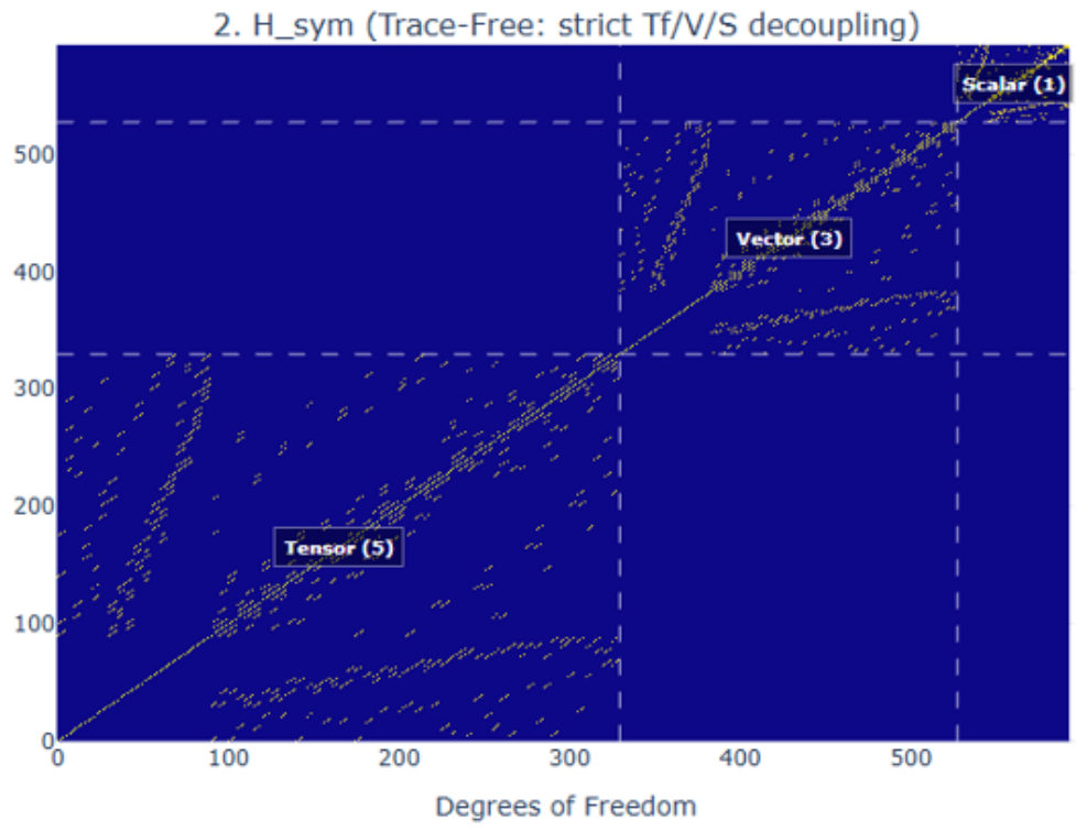
Figure 2.
Finite-mesh projection of the refined octahedral horizon onto the six pole channels . The stationary weights converge to , so gives the homogeneous distinguishability loss . The calculation checks the geometric factor entering the coherence closure; it does not derive or the first-passage threshold. Computed via [38].
Figure 2.
Finite-mesh projection of the refined octahedral horizon onto the six pole channels . The stationary weights converge to , so gives the homogeneous distinguishability loss . The calculation checks the geometric factor entering the coherence closure; it does not derive or the first-passage threshold. Computed via [38].
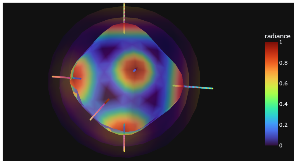
Figure 3.
Scalaron phase-space evolution from six initial conditions. The trajectories converge onto the same attractor before , with a spread in below . No measured primordial observable is fitted. Computed via [38].
Figure 3.
Scalaron phase-space evolution from six initial conditions. The trajectories converge onto the same attractor before , with a spread in below . No measured primordial observable is fitted. Computed via [38].
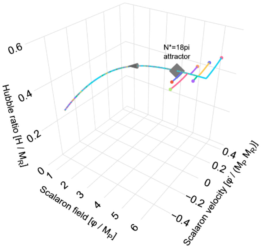
Figure 4.
Dynamical audit of the one-resolution closure. At , the scalaron integration gives , approaching unity deeper on the plateau and supporting percent-level consistency with . Computed via [38].
Figure 4.
Dynamical audit of the one-resolution closure. At , the scalaron integration gives , approaching unity deeper on the plateau and supporting percent-level consistency with . Computed via [38].
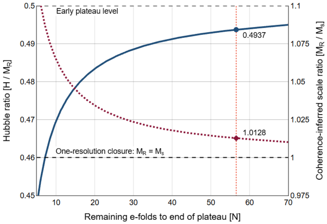
Figure 5.
Numerical Hubble-flow trajectory extracted from the integrated scalaron background, compared with the leading-order plateau relation. At , the numerical solution gives and , while the leading-order relations give and . Their gradual separation toward lower measures the finite- correction. Computed via [38].
Figure 5.
Numerical Hubble-flow trajectory extracted from the integrated scalaron background, compared with the leading-order plateau relation. At , the numerical solution gives and , while the leading-order relations give and . Their gradual separation toward lower measures the finite- correction. Computed via [38].
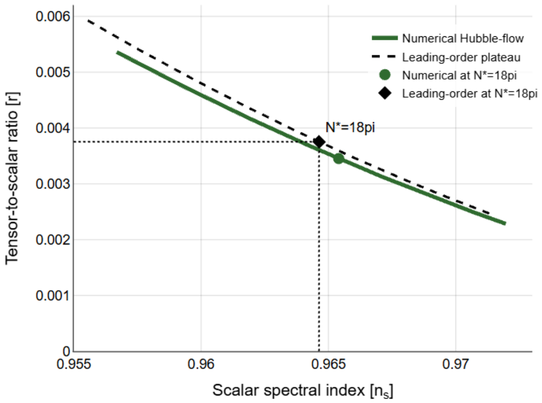

Table 1.
Fixed minimal-sector architectural ingredients used in the phenomenological audit.
| Ingredient | Fixed structure | Published origin | Used below in |
|---|---|---|---|
| Axiomatic architecture | Axioms P1–P7 | [1] | Minimal boundary sector |
| Operational locality | [1] | Local trace domain | |
| Boundary completion | waist | [1] | Edge data and gluing |
| Finite resolution | [1] | Physical bandwidth | |
| Modular history | [1] | Heat-kernel response | |
| Waist topology | [1] | Capacity prescription | |
| Tip defect | [1] | Capacity, coherence, leakage | |
| Spin/twist closure | [1] | Spinorial structure | |
| Topology-locked capacity | and N | [1] | Boundary response depth |
| Coherent tensor depth | [1] | Gravitational stiffness | |
| Constitutive relation | [1] | Newton calibration | |
| Physical matching scale | [1] | All sectoral targets |
Table 2.
Fixed dynamical structures used in the phenomenological audit.
| Ingredient | Fixed structure | Published origin | Used below in |
|---|---|---|---|
| Operational domain | [1], Sec 2.1 | Common trace domain | |
| Relative entropy | [1], Sec 2.1 | Mismatch functional | |
| Matched KMS state | [1], Sec 2.2 | Quadratic response | |
| Kubo–Mori Hessian | [1], Sec 2.2 | Stiffness matrix | |
| Sector split | [1], Sec 2.2 | Orthogonal separation | |
| Spectral volume | [1], Sec 2.3 | Four-volume extraction | |
| Tensor response | [1], Sec 2.4 | Plateau cosmology | |
| Vector response | () | [1], Sec 2.5 | Current normalization |
| Scalar response | [1], Sec 2.6 | Mass deformation | |
| Lagrangian | [1], Sec 2.7 | Effective action | |
| CPTP update | [1], Sec 2.9 | Open-modular dynamics | |
| Walsh filtration | [1], Sec 2.9 | Matter generation carrier | |
| Lie filtration | [1], Sec 2.9 | Lepton accessibilities |
Table 3.
Phenomenological output ledger and epistemic classification.
| Quantity | Framework Output | Benchmark | Comparison | Audit |
|---|---|---|---|---|
| Cosmology: Coherence, Capacity, and Entropic Response (Section 5) | ||||
| Scalaron mass | [68] | |||
| Plateau stiffness | [68] | |||
| Coherence | – | – | ||
| Scalar tilt | [68] | |||
| Tensor ratio r | [70] | Consistent | ||
| Scalar amplitude | [68] | |||
| BH threshold | – | – | ||
| Vacuum | [74] | |||
| Struct. growth | [68,76] | Consistent | ||
| Accel. floor | [77,78] | Consistent | ||
| Electroweak Saturation Relations (Section 6.1) | ||||
| Higgs mass | [74] | |||
| VEV v | [74] | |||
| Top mass cap | [74] | |||
| Top Yukawa | [74] | |||
| Higgs quartic | [74] | |||
| Gauge Couplings as Entropic Stiffness (Section 6.2) | ||||
| Strong | [74,81] | |||
| EM | [81] | |||
| Weak-mixing | [74,81] | |||
| Internal lock | [81] | |||
| Fine-structure | [84] | |||
| Lepton Mass Spectrum via Spectral Filtration (Section 6.3) | ||||
| Proton mass | [74] | |||
| Electron mass | [74] | |||
| Muon mass | [74] | |||
| Tau mass | [74] | |||
| Quark Yukawa Hierarchy (Section 6.4) | ||||
| Bottom | [101] | |||
| Charm | [101] | |||
| Strange | [101] | |||
| Down | [101] | |||
| Up | [101] | |||
Disclaimer/Publisher’s Note: The statements, opinions and data contained in all publications are solely those of the individual author(s) and contributor(s) and not of MDPI and/or the editor(s). MDPI and/or the editor(s) disclaim responsibility for any injury to people or property resulting from any ideas, methods, instructions or products referred to in the content. |
© 2026 by the authors. Licensee MDPI, Basel, Switzerland. This article is an open access article distributed under the terms and conditions of the Creative Commons Attribution (CC BY) license (http://creativecommons.org/licenses/by/4.0/).
Copyright: This open access article is published under a Creative Commons CC BY 4.0 license, which permit the free download, distribution, and reuse, provided that the author and preprint are cited in any reuse.