

Submitted:
26 August 2026
Posted:
02 September 2026
You are already at the latest version
Abstract
We prove two deterministic inapproximability results. First, for every fixed \(0<\epsilon<1/2\), Euclidean \(\mathrm{GapCVP}^{(2)}\) is NP-hard with gap factor \(n^{1/2-\epsilon}\) under deterministic polynomial-time many-one reductions, where \(n\) denotes the lattice rank. Consequently, the Euclidean closest vector problem is NP-hard to approximate within the same factor. This improves the previous \(n^{1/400}\) hardness factor in Chapter 7 of the OpenAI report [Ope25]. Aharonov and Regev gave short certificates for both the YES and the NO case of \(\operatorname{GapCVP}^{(2)}\) at gap factor \( C\sqrt n \), placing that problem in \(\mathrm{NP}\cap\mathrm{coNP}\) for an absolute constant \(C>0\) [AR05]. An NP-hard problem lying in \(\mathrm{coNP}\) would give \(\mathrm{NP}=\mathrm{coNP}\), so the factor \(n^{1/2-\epsilon}\) above cannot be improved to \( C\sqrt n \) unless the two classes coincide. Second, for every fixed \(0<\epsilon<1\), the gap versions of binary nearest codeword and binary syndrome decoding are NP-hard with factor \(n^{1-\epsilon}\) under deterministic polynomial-time many-one reductions, where \(n\) denotes the binary block length. Consequently, both optimization problems are NP-hard to approximate within the same factor. This improves the previous \(n^{1/200}\) hardness factor in Chapter 7 of the OpenAI report [Ope26].
Keywords:
complexity
; hardness
1. Introduction
The gap version of the closest vector problem provides the standard decision formulation for studying approximation hardness. Let be nonsingular. Its columns generate the full-rank lattice , whose rank is n. Given a target and a norm , the optimization version of the closest vector problem asks for minimizing ; see Micciancio and Goldwasser [MG02, Chapter 3] for standard background.
For an approximation factor and a positive rational radius r, the promise problem asks one to distinguish
where . Instances whose optimum lies between the two thresholds are outside the promise. A -approximation algorithm for the optimization problem solves this promise problem by comparing the distance of its output with . Thus NP-hardness of rules out such an approximation algorithm unless .
The Euclidean closest vector problem is the specialization to the norm. We write
and denote its gap version by . Van Emde Boas [vEB81] proved NP-hardness of exact Euclidean CVP. Arora, Babai, Stern, and Sweedyk [ABSS97] established hardness within every fixed constant. For every fixed , they also proved hardness within under the assumption [ABSS97]. Dinur, Kindler, and Safra [DKS98], in work subsequently refined by Dinur, Kindler, Raz, and Safra [DKRS03], strengthened this to for some absolute constant . Although this factor dominates every fixed power of , its exponent tends to zero and hence does not give hardness for any fixed . The OpenAI report [Ope26, Chapter 7] subsequently obtained the fixed polynomial factor by a deterministic reduction from 3SAT. Fixed-polynomial lattice inapproximability had previously been obtained conditionally on the Projection Games Conjecture by Moshkovitz [Mos15, Section 5.1] and Mukhopadhyay [Muk22]. Those conditional results are qualitatively different from the unconditional deterministic reduction from ordinary 3SAT proved here. The Exponential Time Hypothesis (ETH), introduced by Impagliazzo and Paturi [IP01], has also served as the basis for recent fine-grained lower bounds for constant-factor approximations of CVP and related problems [AGMZ26,HKW26]. These results concern the running time of constant-factor approximation rather than unconditional NP-hardness for polynomial approximation factors.
The square-root scale forms a complexity-theoretic barrier. Goldreich and Goldwasser [GG00] established interactive-proof upper bounds that constrain the nonapproximability of lattice problems. Aharonov and Regev [AR05] subsequently proved that, for some absolute constant ,
Consequently, NP-hardness at that scale under deterministic polynomial-time many-one reductions would imply . The reduction given here achieves every fixed exponent below .
Binary nearest codeword is an optimization problem over . Given a k-dimensional binary linear code and a target word , the task is to find a codeword in C minimizing its Hamming distance from y [BMT78]. Binary syndrome decoding takes as input a binary parity-check matrix H and a syndrome , and asks for a minimum-weight binary vector e satisfying [BMT78]. The two formulations are equivalent. Indeed, if and , then the map identifies codewords with vectors e satisfying . Consequently, the two instances have the same optimum value, and the correspondence preserves approximation ratios. Conversely, given a consistent syndrome instance , Gaussian elimination finds y with , and the same correspondence reduces it to nearest codeword for .
Berlekamp, McEliece, and van Tilborg [BMT78] proved that binary syndrome decoding is NP-complete. For binary nearest codeword, Arora, Babai, Stern, and Sweedyk [ABSS97] proved unconditional NP-hardness of approximation within every constant factor. For every fixed , they also proved hardness within under the assumption that NP has no quasipolynomial-time algorithms, namely . Arora’s thesis [Aro94, Section 6.4] gives a contemporaneous account and explicitly records the stronger exponent for nearest codeword. For nearest codeword with preprocessing, Alekhnovich, Khot, Kindler, and Vishnoi [AKKV05] proved hardness within under the same quasipolynomial-time assumption. Khot, Popat, and Vishnoi [KPV14] strengthened the factor to under . For ordinary nearest codeword, Bhattiprolu, Guruswami, and Ren [BGR25] subsequently gave a PCP-free proof of the same two bounds: unconditional NP-hardness within every constant factor and hardness under the assumption that NP has no quasipolynomial-time algorithms. Their contribution is a new proof rather than a stronger approximation factor. Bhattiprolu, Guruswami, Lee, and Ren [BGLR25] subsequently studied the inapproximability of finding sparse vectors in codes, subspaces, and lattices via randomized reductions; their lattice result does not yield deterministic fixed-polynomial hardness for Euclidean CVP. Methodologically, Bennett and Peikert [BP23] also combine Reed–Solomon codes [RS60] with an integer-lattice lift to obtain randomized hardness for approximate SVP and identify derandomization as a central obstacle.
Bitansky, Harsha, Ishai, Rothblum, and Wu [BHI+24] showed that ETH rules out -time approximation within a certain constant factor, using the equivalent formulation that minimizes the number of unsatisfied linear equations. Subsequently, Corollary 15 of the OpenAI report [Ope26] established, without an additional complexity assumption, NP-hardness of approximation within for binary nearest codeword and binary syndrome decoding under deterministic polynomial-time many-one reductions. The result proved here uses the same unconditional reduction model and improves the approximation factor to for every fixed .
On the algorithmic side, Alon, Panigrahy, and Yekhanin gave several deterministic approximation algorithms and time–ratio tradeoffs [APY10]. Their general polynomial-time algorithm achieves an approximation. Berman and Karpinski gave, for every fixed constant , a deterministic algorithm with approximation factor and a randomized algorithm with factor [BK02]. Alon, Panigrahy, and Yekhanin observed that the latter analysis yields approximation factor [APY10].
1.1. Our Results
We first record the two Euclidean lattice problems used below.
Definition
(Euclidean closest vector). An instance consists of a nonsingular matrix and a target . The matrix B generates the full-rank lattice . The objective is to output a vector minimizing . Its optimum value is .
Definition
(Euclidean GapCVP). Let . An instance of consists of a nonsingular matrix , a target , and a radius . It is promised that either , which is the YES case, or , which is the NO case. The task is to distinguish the two cases.
We now state our main Euclidean result. It improves the hardness factor in Theorem 1 on page 184 of the OpenAI report [Ope26].
Theorem 1.3
(Euclidean closest vector, informal version of Theorem 8.1). For every fixed , there is a deterministic polynomial-time mapping that assigns to each 3SAT formula φ a nonsingular matrix , a target , and a radius such that
Consequently, is NP-hard under deterministic polynomial-time many-one reductions.
Remark 1.4.
Our Theorem improves the Euclidean closest-vector hardness factor established in Theorem 1 of the OpenAI report [Ope26] to . Aharonov and Regev proved that lies in for an absolute constant [AR05]. No NP-hardness result under deterministic polynomial-time many-one reductions can reach that scale unless .
We next formally define the two binary problems.
Definition
(Binary nearest codeword). An instance consists of a binary linear code , given by a generator matrix, and a target word . The objective is to output a codeword minimizing . We denote the optimum value by
Definition
(Binary syndrome decoding). An instance consists of a binary matrix and a syndrome . The objective is to output a vector of minimum Hamming weight subject to . We denote the optimum value by
To state approximation hardness, we use the gap versions of these two optimization problems. Both are promise problems parameterized by a radius and an approximation factor.
Definition
(Binary gap nearest codeword and gap syndrome decoding). Let . An instance of is a binary nearest-codeword instance together with a positive integer radius R; it is promised that either or . An instance of is a binary syndrome-decoding instance together with a positive integer radius R and the analogous promise or . In both cases n is the binary block length, and the task is to distinguish the two promised cases.
The following theorem improves the hardness factor established by Corollary 15 on page 213 of the OpenAI report [Ope26].
Theorem 1.8
(Main result, informal version of Theorem 7.1). For every fixed , and are NP-hard under deterministic polynomial-time many-one reductions, where n is the binary block length. Consequently, binary nearest codeword (Definition 1.5) and binary syndrome decoding (Definition 1.6) are NP-hard to approximate within .
2. Technique Overview
This section compares the mechanism behind the OpenAI reduction [Ope26] with the two quadratic estimates that permit a sharper choice of parameters. We focus on the reduction to binary nearest codeword and syndrome decoding (Theorem 1.8). The Euclidean closest-vector result (Theorem 1.3) then follows from the dimension-preserving parity-lift reduction, which converts a binary weight gap into the square root of that gap in Euclidean distance. Section 2.1 reviews the approach in the OpenAI report, whereas Section 2.2 explains how our sharper analysis improves the resulting hardness factors.
2.1. Overview of the OpenAI Approach
Chapter 7 of the OpenAI report [Ope26] factors the reduction as
The first arrow contains the main algebraic construction. Let be the input formula, let s be its encoding length, and let m and ℓ be its numbers of variables and clauses. We define and . The variables are indexed by and represented by distinct anchors in a characteristic-two field . A Boolean assignment determines the unique polynomial of degree less than m satisfying , where is the bit assigned to variable i. The reduction evaluates this polynomial on .
The binary variables are arranged into evaluation tables. For a clause C, let be the set of its variable indices and let be its satisfying local assignments. The table types are : type 0 is the global table, and is the subtype asserting that clause C receives the local assignment . Write for the binary coordinate selecting the field value in table at , and define its fiber by .
Fix a moment budget T. For , the ordinary power sum of table at p is
For , , and , the shifted power sum is
where is the bit assigned to variable i by . The affine constraints require these pointwise quantities to be evaluations of low-degree polynomials and require the clause tables to reproduce the global table modulo two. Let denote the resulting binary affine system, let be its number of binary coordinates, and, when the system is consistent, define If satisfies the formula, each active fiber is the singleton , exactly one subtype is active for every clause, and the resulting binary solution has weight .
For soundness, start with a low-weight binary solution. For a fiber cutoff , define the good evaluation set of table by . Markov’s inequality shows that contains all but a small set of evaluation points. Reed–Solomon interpolation turns the pointwise moments into polynomials in the indeterminate X. Lemma 10 of the OpenAI report [Ope26] uses the associated Hankel matrix to construct a monic separable polynomial . Its roots in a common splitting field have the prescribed power sums. The shifted moments are then examined using a valuation above . They force every root associated with subtype to reduce to the bit at the anchor . Finally, the clause decomposition and a Vandermonde argument match a global root with a satisfying subtype for every clause. Using the same valuation for a variable wherever it occurs makes these local assignments consistent, producing a global satisfying assignment.
The three parameters , T, and q serve different purposes, but the soundness proof couples them. The cutoff must be large enough that a low-weight solution has few heavy fibers: if , then
Increasing improves this estimate, but it makes both algebraic steps more expensive. Thus one cannot choose the cutoff, the moment budget, and the field size independently.
Lemma 12 of the OpenAI report [Ope26] uses a large moment budget because of its local valuation argument. For a reconstructed polynomial of degree , it first bounds the coefficients of an inverse Vandermonde matrix. In the notation of that argument, the successive bounds are
With and , these quantities have scales , , and , respectively. The proof uses the moments with indices from z through to isolate one root at a time. Consequently, the moment budget must be larger than this range; the choice provides ample slack. This is the local-valuation moment cost; it does not come from the Reed–Solomon encoding itself.
Lemma 10 of the OpenAI report [Ope26] imposes two further costs, both quadratic in the fiber cutoff. Its Hankel determinant has degree at most ; hence, uniformly for , as many as retained sample points may fail to have maximum fiber size. Moreover, after clearing the common denominator , the j-th root-moment discrepancy has degree at most , which is bounded by for . Thus the reconstruction lemma requires
We call the subtractive term the determinant-zero cost and the right-hand term the denominator-clearing cost. For , , and , the right-hand side is of order . Hence the field must be substantially larger than . Moreover, it must remain large after the heavy fibers are discarded. Taking makes both requirements hold with considerable uniform slack: since and , the preceding discarded-point bound is for the target factor . The exact exponents 30 and 200 are therefore deliberately generous choices, but the original proof genuinely requires a large separation among these scales.
Finally, gives . Soundness against solutions of weight yields the coding gap. The standard parity lift outputs a lattice basis B and a target t satisfying , so this becomes the Euclidean gap.
2.2. Overview of Our Approach
We retain the outer reduction through a sparse binary affine system, but replace its inner encoding and soundness mechanism. Multi-axis exponent reconstruction replaces anchor-based interpolation, and soundness is proved by a high-rank/low-rank dichotomy combining rank charging with short-recurrence atomization.
Sparse quadratic encoding and assignment compression. Instead of interpolating an assignment by a polynomial through anchors, we first replace the formula by a system of homogeneous quadratic forms in which each form has at most five monomials (Lemma 3.2), and we then compress an assignment into one field element, where the are independent over , so that is injective. Consistency between occurrences of a variable is enforced by linear equations in the quadratic encoding rather than by a valuation at an anchor, so no local analysis at anchors is needed at any point below.
Axis-wise interpolation and multi-axis exponent reconstruction. Fix a power of two d and a number of axes r, and put . For each axis j the reduction uses the polynomial of degree less than with , which exists because is a basis, and whose coefficients are -linear in x because is a power of two and the Frobenius map is additive (Lemma 3.3). Writing an exponent in base d as gives by Lemma 3.4. This is the quantitative heart of the construction: r axis polynomials represent consecutive powers of the assignment encoding, while the interpolation degree needed to carry them grows only linearly in d. Thus the construction represents consecutive powers while the interpolation-degree dependence on the radix remains linear in d.
The table has one block for every pair , every label ℓ in the label set , and every sample point s in the sample set ; for fixed ℓ and s these form a block .
Definitions 3.7 and 3.9 introduce the derived quantities f, F, and u.
From interpolants to exponent-indexed moments. Definition 3.8 controls how the table is converted into scalar moments. The degree bound keeps interpolation within the available budget, while the consistency condition ensures that depends only on the scalar exponent . Thus the exponent-indexed moments are well defined.
Algebraic identities of honest moments. Definition 3.10 imposes the three algebraic identities satisfied by honest moments. Doubling an exponent squares the moment, the linear-combination identity advances the exponent through the assignment encoding, and matrix-inner-product vanishing enforces every quadratic encoding form. These constraints are affine over ; in particular, squaring is affine because it is the Frobenius automorphism (Lemma 3.12).
Direct constraints on table blocks. Definition 3.11 acts directly on the table blocks. Symmetry makes each block behave like a matrix of pairwise products, while anchor normalization fixes the homogenizing coordinate and removes the scaling ambiguity. Accordingly, the completeness witness places one rank-one block at the honest label of each sample point (Lemma 3.13).
Charging rank instead of discarding a discriminant. Soundness splits on the rank of the polynomial moment matrix over . If that rank is at least , we do not ask any determinant to be nonzero at any particular sample point. Instead we choose one minor with nonzero determinant , note that the rank lost at a sample point s divides to that order, and sum:
Here the Kronecker factorization gives the first inequality (Lemma 4.1). Determinantal divisibility gives the second: if , then , and therefore (Lemma 4.3). For fixed r, is linear in the radix d, equivalently proportional to up to the displayed factors; in particular, no quadratic -factor appears. Thus the high-rank branch replaces the determinant-zero cost in Eq. (1). Rather than discarding every sample point where a maximal-fiber Hankel determinant vanishes, it charges each pointwise rank deficit to the vanishing order of one fixed nonzero minor.
Atomization instead of local valuation. In the complementary case the rank is below , so every scalar moment sequence obeys a short linear recurrence (Lemma 5.2). View the sequence as a functional g on the finite-dimensional recurrence algebra it generates. Before passing to the reduced algebra, generalized nilpotent components may still occur, while arbitrary coefficients could permit cancellation between candidate assignments. The doubling-is-squaring identity in Definition 3.10-(a) removes exactly these freedoms: the identity makes g vanish on the nilradical and forces the idempotent values to satisfy , hence to lie in . So every moment sequence is a plain sum over an entrywise set of distinct atoms with all coefficients equal to one (Lemma 5.3). Constraint-local Vandermonde isolation then synchronizes these entrywise atom sets and decodes a satisfying assignment (Lemma 6.2). This low-rank branch avoids the denominator-clearing cost in Eq. (1): the atom identities are proved inside the recurrence algebra and synchronized by a constraint-local Vandermonde system, rather than by inverse-Vandermonde local valuation followed by interpolation of a denominator-cleared global root identity.
Nearest codeword and syndrome decoding. A light table therefore yields a satisfying assignment, so an unsatisfiable formula forces weight at least , whereas completeness costs only . The block length is , because the table has one sample coordinate, r label coordinates, and one matrix block. The actual gap satisfies . With and , the block length is , whereas . Thus the gap exponent is , which approaches as for fixed r and then can be made arbitrarily close to 1 by choosing r large. Consequently, for every fixed , the reduction gives an gap for binary nearest codeword and syndrome decoding (Theorem 7.1).
Euclidean GapCVP. The parity-kernel lattice lift identifies Hamming weight with squared Euclidean distance exactly, through . Taking square roots halves the binary gap exponent. Because the binary theorem permits arbitrary slack, reserving part of it for radius rounding yields an hardness factor for Euclidean GapCVP for every fixed (Theorem 8.1). That endpoint is the square-root scale of Aharonov and Regev [AR05], which no reduction of this kind can reach unless .
2.2.0.1. Roadmap.
Section 3 defines basic notation, reduces 3SAT to a sparse quadratic system, introduces the assignment encoding and the folded axis polynomials, defines the binary affine system, and proves completeness. Section 4 proves the rank-charging bound for tables whose moment matrix has large rank. Section 5 proves that in the complementary case the moment sequences are sums over entrywise sets of fewer than atoms with unit coefficients. Section 6 combines the two cases and decodes an atom into a satisfying assignment. Section 7 chooses the parameters and proves the hardness result for binary nearest codeword and binary syndrome decoding. Section 8 lifts the binary instance to a full-rank integer lattice while preserving the optimum as a squared Euclidean distance, which gives the hardness result for Euclidean GapCVP.
3. Preliminaries and The Binary Affine System
Section 3.1 defines basic notation and field conventions. Section 3.2 introduces index maps and bounded lifts; Section 3.3 converts 3SAT into a sparse quadratic encoding; Section 3.4 develops axis-wise interpolation and multi-axis exponent reconstruction; and Section 3.5 assembles these ingredients into the binary affine system and establishes its completeness properties.
3.1. Notation
For a positive integer n, we define . We write for the integers and for the real numbers. For a matrix A, denotes its transpose and its rank. If A is square, denotes its determinant. For matrices A and B, denotes their Kronecker product, so that .
For a vector , its Hamming weight is , and the same notation is used for the number of nonzero entries of a matrix. For binary vectors , their Hamming distance is . For a nonempty set , we define . For , its Euclidean norm is , and for and a nonempty we define . In every application below, V is a lattice or a finite set, so the infimum is attained.
Throughout, q is a power of two and . We write and for the polynomial ring and the rational-function field over . For a nonzero , denotes its degree, and we set . defines basic notation and field conventionsFor , denotes the order of vanishing of at .
3.2. Index Maps and Bounded Lifts
To formulate the affine system, we need to translate bounded multi-indices into scalar exponents and back. The following index and lift maps provide this translation while respecting the prescribed coordinate range.
Definition
(Index map and bounded lift). Fix a power of two , an integer , and an integer . For a multi-index , its exponent index is
For every integer , the bounded lift
is the multi-index obtained by greedily expanding a from the highest base-d position to the lowest. It is chosen so that
Thus ind converts a multi-index into its scalar exponent, while selects a bounded multi-index representing a given scalar exponent.
The bounded lift exists throughout the stated range. Indeed, the largest attainable index is . Set and process , maintaining . At position h, choose
If the cap is inactive, then . If it is active, then . Thus the invariant propagates, and at it gives . When , this is the ordinary base-d expansion. Moreover, linearity of the index map gives
whenever both bounded lifts are defined.
3.3. Sparse Quadratic Encoding
Let be a 3SAT formula of encoding length N. Delete tautological clauses, repeated literals, and unused variables. If deleting repeated literals leaves a clause with fewer than three literals, repeat one of the survivors until it has exactly three; this changes neither the truth value of the clause nor the analysis below, in which two of the three falsity bits then coincide. The cases of an empty clause and of no remaining clauses are handled by fixed promise instances.
Give every occurrence of a variable its own bit, and tie the occurrences of one global variable to its lexicographically first occurrence by equalities. This keeps the number of equalities linear in the number of occurrences, rather than quadratic. For a clause with falsity bits , introduce one auxiliary bit y and impose and . Adjoin one homogenizing coordinate and let collect it together with all occurrence and auxiliary bits, where is the homogenizing coordinate. For each falsity bit , let be or , according as the corresponding literal is negated or unnegated. The clause equations become and , while an occurrence equality becomes . Thus every constraint above becomes a homogeneous quadratic form with at most five nonzero coefficients, since each falsity bit is either a coordinate or the sum of a coordinate and . Let be the encoding forms. Both n and L are .
Lemma
(Sparse quadratic encoding). The formula φ is satisfiable if and only if there is such that satisfies for every .
Proof.
Set . The equalities force all occurrences of one global variable to agree, so the occurrence bits define a Boolean assignment, and conversely. Fix a clause and its falsity bits. If , then the first equation forces and the second holds for every . If , then the first equation forces and the second forces , so the third literal is true. If , the two equations are inconsistent. Hence the pair is solvable in y exactly when , which is exactly the condition that the clause is satisfied. □
3.4. Axis-Wise Interpolation and Multi-Axis Exponent Reconstruction
Let be an extension of of degree , generated by , and chosen so that . Fix that are linearly independent over ; such elements exist because . For , we define the assignment encoding
Since the are independent over , the map is injective.
We define the moment threshold . The point of the reconstruction is that consecutive powers of are carried by r axis polynomials whose degrees grow only with d.
Lemma
(Axis-wise interpolation). For every and every there is a unique with and . Its coefficients are -linear functions of x.
Proof.
The set is a -basis of , so every element of is for a unique of degree less than c, which gives existence and uniqueness. Since is a power of two and , the Frobenius map gives
Writing with gives , whose coefficients are -linear in x. □
Lemma
(Multi-axis exponent reconstruction). For every and every ,
Proof.
By Lemma 3.3, the h-th factor contributes exponent to . The total exponent is therefore , proving the claim. □
3.5. The Binary Affine System
We define the sample set and the label set . The synchronization step of Section 6 isolates atoms against a union of at most atom sets, so the moment window has to be wider than . We collect the resulting budgets in one definition.
Definition
(Window and degree parameters). We use four named budgets because different stages of the proof require different ranges.
First, define the synchronization factor by
It provides enough slack to combine the atom sets arising from the at most matrix entries in a linear-combination equation.
Second, define the isolation-window length by
This is the number of Hankel rows. The soundness proof uses the consecutive moments with indices for recurrence propagation and Vandermonde isolation.
Third, define the largest exposed moment index by
The affine system exposes moments with indices . Thus is an endpoint, rather than the length of an isolation window.
Finally, define the degree budget by
It bounds the degrees of the interpolants obtained from products of the r axis polynomials: each admissible exponent is at most and each axis polynomial has degree less than c.
We require and . The latter condition gives .
These four budgets determine both the allowed digit range and the moment indices exposed by the affine system. We now collect the multi-indices whose coordinates respect that range.
Definition
(Admissible multi-indices). The admissible multi-index set is
For every , we have , so every admissible exponent lies in the exposed moment range.
For the row and column indices used below, we abbreviate for .
For every and the system has one binary variable
so a coordinate of the system is named by a row index i, a column index j, a label ℓ, and a sample point s. For fixed ℓ and s these variables form the block whose entry is , and the whole table is denoted . The number of binary coordinates is therefore
Definition
(Weighted interpolants).
The following quantities are derived linearly from the table . For , , and , the table is read through
For every and every , let be the unique polynomial of degree less than q satisfying for every . Such a polynomial exists and is unique because has q distinct points.
These interpolants package the dependence on the sample point s into the polynomial variable X. We next bound their degrees and require that evaluation at depend only on the exponent encoded by the multi-index.
Definition
(Degree and exponent consistency). The following two families constrain the interpolants.
- (a)
- Bounded degree. For every and every ,
- (b)
- Index-fiber consistency. For every and all with ,
When these constraints hold, any two multi-indices with the same ind give the same value at . This allows us to replace the multi-indexed evaluations by a single sequence indexed by the scalar exponent k.
Definition
(Exponent-indexed moments). For each , fix once and for all a representative with ; such representatives exist by the greedy construction above with . For every , we define
Whenever the index-fiber consistency constraint holds, this equals for every with .
The quantities are the scalar moments used in the soundness argument. We now impose the algebraic identities satisfied by the honest moments, coming from the doubling-is-squaring identity, the linear-combination identity, and the quadratic encoding.
Definition
(Algebraic moment constraints). These three families constrain the moments. Let be the index budget defined in Definition 3.5.
- (a)
- Doubling is squaring. For every and every k with ,
- (b)
- Linear combination. For every and every k with ,
- (c)
- Matrix inner product is zero. For every and every ,
The preceding conditions constrain the table only through its derived moments. Two final conditions act directly on the table blocks, enforcing symmetry and normalizing the anchor entry.
Definition
(Table symmetry and normalization). The following two families constrain the entries of the table directly, without passing through the moments.
- (a)
- Symmetry in the matrix indices. for all i, j, and .
- (b)
- Row summation in is one. for every .
The binary affine system consists of the two families of Definition 3.8, the three families of Definition 3.10, and the two families of Definition 3.11.
Lemma
(The system is affine). Every condition in Definitions 3.8, 3.10, and 3.11 is an affine condition over on the table bits.
Proof.
Each is a fixed -linear combination of table bits, hence an -linear function of them; interpolation on and evaluation at are -linear and therefore -linear. Writing
each coefficient is an -linear function of the table bits. Family Definition 3.8-[item:degree](a) is precisely the vanishing of these coefficients for . Evaluation also shows that every is an -linear function of the table bits. The remaining families Definition 3.8-[item:folding](b), Definition 3.10-[item:identifier](b), Definition 3.10-[item:source](c), Definition 3.11-[item:symmetry](a), and Definition 3.11-[item:anchor](b) are then -linear or affine by inspection. For Definition 3.10-[item:frobenius](a), the map is the Frobenius automorphism of , which is -linear, so is an -linear function of the table bits as well. Expanding each -valued equation in an -basis of turns every family into binary affine equations. □
Let denote the resulting binary affine system, where collects the table bits.
Lemma
(Completeness). If φ is satisfiable, then has a binary solution of weight at most
Proof.
Let be as in Lemma 3.2 and put . At each sample point s, we define the honest label
and we set and for . Exactly one block is nonzero at each sample point, so the weight is , which gives Eq. (3).
We verify the seven families. For every ,
and the polynomial has degree at most by Lemma 3.3, so it is the unique interpolant of Definition 3.7, so ; in particular, Definition 3.8-[item:degree](a) holds. Evaluating at and applying Lemma 3.4 gives
which depends only on and hence gives Definition 3.8-[item:folding](b). For Definition 3.10-[item:frobenius](a),
where the first step follows from Eq. (4), the second step follows from and together with the fact that squaring is additive in characteristic two, and the third step follows again from Eq. (4). For Definition 3.10-[item:identifier](b),
where the first step follows from Eq. (4) and for , the second step follows from the definition of , and the third step follows from Eq. (4) and . For Definition 3.10-[item:source](c), by Lemma 3.2. Family Definition 3.11-[item:symmetry](a) holds because is symmetric, and Definition 3.11-[item:anchor](b) holds because . □
4. Rank Loss and Determinantal Charging
A low-weight table cannot support a moment matrix of large rank. The reason is that rank is subadditive and is bounded by the number of nonzero bits, while a determinant of a large minor cannot vanish to high order at too many sample points. Charging the amount of rank lost at each sample point, rather than merely whether rank is lost there, is what keeps the estimate linear in the moment threshold.
We define the polynomial block matrix , with rows indexed by and columns by for , , and , by
This is well defined: the entries of are at most , so , and . Consequently, whenever the index-fiber consistency family Definition 3.8-[item:folding](b) holds, . The row window is wider than the column window, which is what the synchronization step of Section 6 consumes.
Lemma
(Specialization). For every , define and by and . Then, for every ,
Proof.
By Definition 3.7, the polynomial agrees with at every , so
where the first step follows from the definition of applied to , and the second step follows from the definitions of and . This is the asserted Kronecker decomposition. Taking ranks,
where the first step follows from subadditivity of rank, the second step follows because a Kronecker product with a rank-one matrix does not increase rank, and the third step follows because every matrix is the sum of as many rank-one matrices as it has nonzero entries. □
To aggregate rank losses across the sample points, we need a local connection between specialization rank and determinant vanishing. The next lemma provides this connection: a rank deficit forces the determinant to vanish to order at least at .
Lemma
(Determinantal divisor). Let and , and define . If , then divides .
Proof.
Localize at . The ring is a discrete valuation ring, so C admits a Smith normal form with invertible over that ring and diagonal with entries . Specializing at gives , so at least of the exponents are positive, and therefore . □
The preceding lemma measures the rank lost at a sample point by the zero multiplicity of a nonzero minor. Summing these multiplicities over all sample points charges the total rank deficit to the degree of that minor, yielding the global weight bound below.
Lemma
(Rank charging). Suppose the table satisfies Definition 3.8-[item:degree](a) and . Define . Then
Proof.
Since the rank is at least , there is a submatrix of with . Every entry of has degree at most by Definition 3.8-[item:degree](a), so . Setting , Lemma 4.2 gives for every , and distinct sample points give coprime factors, so
Therefore
where the first step is the definition of the total weight, the second step follows from Lemma 4.1, the third step follows because is a submatrix of , the fourth step follows from the definition of and , and the fifth step follows from the displayed bound on . □
5. Short Recurrences and Atomic Moments
We now treat the complementary case, in which the moment matrix has rank below . A short recurrence gives a finite-dimensional recurrence algebra, which may initially contain generalized nilpotent components and arbitrary coefficient weights. The doubling-is-squaring condition in Definition 3.10-[item:frobenius](a) kills the nilradical and forces every surviving coefficient to be one, so each entrywise sequence is the plain sum over a set of fewer than atoms. No bound on the global union is needed; synchronization later uses only constraint-local unions.
Lemma
(Atomization). Let have characteristic two and let be a sequence in satisfying a monic linear recurrence with characteristic polynomial of degree , and suppose for every . Then there is a set Ξ of at most ρ distinct roots of χ in a splitting field with
Proof.
Let be a splitting field of and put . Define by . This is well defined, because the map sending to annihilates every multiple of , which is precisely the recurrence at every shift.
We first show for every . Writing and using that squaring is additive in characteristic two, , so
where the first step follows from the definition of g, the second step follows from the hypothesis , available because , the third step follows again from additivity of squaring, and the fourth step follows from the definition of g.
Next, g vanishes on the nilradical of . Indeed, let be nilpotent. Some power with vanishes, and iterating the previous paragraph gives , so because is a field.
Consequently g factors through , where denotes the ideal of nilpotent elements of . By the Chinese remainder theorem, is a product of t copies of , one for each of the t distinct roots of , where . Let be the primitive idempotents and for . From we get , and in a field this forces .
Finally, the image of T in is , so maps to and . Taking completes the proof, and . □
When the polynomial moment matrix has rank , its entries satisfy algebraic dependencies of bounded order. The next lemma converts this rank deficiency into a short linear recurrence for each scalar moment sequence, providing the starting point for the atomization argument.
Lemma
(Short recurrence). Suppose the table satisfies the index-fiber consistency family Definition 3.8-[item:folding](b) and . Then for every there is a monic linear recurrence of order (where order zero means that the sequence vanishes) satisfied by at every index
Proof.
All minors of of size vanish identically, hence also after substituting , so . By the folding hypothesis, fixing i and j and letting and range gives the Hankel submatrix of , whose rank is therefore at most . Hence its first columns are linearly dependent. Let be minimal such that its columns are linearly dependent; such an index exists because the rank is at most . By minimality are independent, so is a combination of them, which is a monic recurrence of order holding at every row index , that is, at every index with . □
Because the recurrence of Lemma 5.2 is verified at every row index below , the sequence it extends agrees with the true moments on the whole window , and Lemma 5.1 applies with . This gives the following form of the moments. The atom sets are indexed entrywise, and no claim is made that one set serves all entries; the synchronization is carried out constraint by constraint in Section 6, where each constraint couples at most entries.
Lemma 5.2 gives a short recurrence for each moment sequence, but a recurrence alone may still involve arbitrary coefficients and repeated roots. The Frobenius identity removes this ambiguity by forcing the sequence to be a sum of pure exponentials with distinct atoms and unit coefficients, as formalized next.
Lemma
(Atomic moments). Suppose the table satisfies Definition 3.8-[item:folding](b) and Definition 3.10-[item:frobenius](a), and suppose . Then for every there is a set of at most ρ distinct elements of a fixed algebraic closure of with
Consequently, for any set of at most index pairs, the union satisfies .
Proof.
Fix and let be the order supplied by Lemma 5.2. If , then the relation produced there reads for every , and satisfies Eq. (6) on the whole window, so we may assume below. Its characteristic polynomial is called , and the recurrence is valid at every index . Let be the sequence determined by the first moments and by that recurrence. By induction on k, for every , and in particular on the window : the two agree below by construction, and for the recurrence expresses both in the same way from earlier terms.
Since and , . Moreover, whenever , .
For every , both k and lie in the range on which agrees with , and . Hence the doubling-is-squaring condition gives
Thus Lemma 5.1 applies to and produces a set of at most distinct roots of with for every , which is Eq. (6) on the window where and agree.
The final bound is immediate: a union of at most sets of size at most has at most elements, and holds by the choice of and the requirement . □
Remark 5.4.
It is tempting to shorten the argument by writing the block Hankel matrix as with and concluding , which would bound the total number of atoms by and make the synchronization immediate. The standard factorization proving that identity uses linear independence of the vectors . Without this hypothesis the identity need not hold. Over , take the atoms 0, 1, and p with , two moment coordinates , and for each of the three atoms. Then , whereas
has determinant and hence rank one. This is why the argument above keeps the atom sets entrywise and pays for the union with the synchronization factor .
6. Soundness Criterion
We now combine the two cases. If the table is light, rank charging forces the moment matrix to have rank below . Atomization then represents every matrix entry through its own set of fewer than atoms, and constraint-local Vandermonde isolation synchronizes precisely the entries in each linear-combination, symmetry, encoding, or anchor equation and recovers a satisfying assignment.
Lemma
(Isolation). Let be a field, let be finite with distinct elements, and let satisfy for every . Then for every ξ.
Proof.
The system has coefficient matrix , which is a Vandermonde matrix on the distinct elements of and hence invertible. □
The preceding lemmas provide two complementary tools: rank charging rules out low-weight solutions in the high-rank case, while atomization and Vandermonde isolation decode a satisfying assignment in the low-rank case. The next lemma combines these two branches. It shows that every solution lighter than must arise from a satisfiable formula.
Lemma
(Soundness criterion). Assume . Suppose a binary solution of has weight less than . Then φ is satisfiable.
Proof.
Because the binary vector solves , it satisfies Definition 3.8-[item:degree](a). Lemma 4.3 in contrapositive form therefore gives . The solution also satisfies Definition 3.8-[item:folding](b) and Definition 3.10-[item:frobenius](a), so Lemma 5.3 gives entrywise atom sets of size at most with Eq. (6) valid for . We define
and we let , so that for . No bound on the total number of atoms is claimed. Each constraint below couples at most entries, so by Lemma 5.3 the union of the atom sets it involves has fewer than elements, and Lemma 6.1 applies to it on the window .
Symmetry. By Definition 3.11-[item:symmetry](a), for every and . Uniqueness of interpolation gives , and Definition 3.9 hence gives for every . The two entries involve at most atoms, so Lemma 6.1 applied to the differences gives for every .
Linear combination. By Definition 3.10-[item:identifier](b), for every j and every ,
where we used Eq. (6) on both sides of Definition 3.10-[item:identifier](b) and collected the coefficient of . This relation involves the entries and for , whose atom sets have union of size at most . Thus the moments indexed by suffice, and Lemma 6.1 gives
Structure of the coefficient matrices. Fix with . If , then Eq. (7) gives , and the are independent over , so the whole column j vanishes. Hence there is some j with , and for every such j Eq. (7) gives with . Since is injective, this vector is the same for all such j; call it and put . Every column of is therefore , that is, with . Symmetry gives . If then and , contrary to assumption, so and
Encoding equations. By Definition 3.10-[item:source](c), for every encoding form and every , using that has at most five nonzero coefficients and hence involves at most five entries, with at most atoms involved, so Lemma 6.1 gives for every . Substituting Eq. (8) turns this into .
Nonemptiness. By Definition 3.11-[item:anchor](b), for every s, so the interpolant of Definition 3.7 is the constant polynomial 1 and Definition 3.9 gives . By Eq. (6) and Eq. (8), counts modulo two the atoms with , so that number is odd and in particular nonzero.
Pick any with . Then satisfies every encoding form, so is satisfiable by Lemma 3.2. □
7. Hardness of Binary Nearest Codeword and Syndrome Decoding
It remains to choose the parameters. The radix d controls both the moment threshold and the degree budget , but it enters them very differently: grows like , whereas grows only linearly in d. Since the sample field is taken greater than , the gap can be made almost as large as , and the block length pays . The ratio of these two exponents is what produces .
Theorem
(Main result, formal version of Theorem 1.8). Fix an integer and a real . Then and are NP-hard under deterministic polynomial-time many-one reductions, where M is the binary block length. Consequently, binary nearest codeword and binary syndrome decoding are NP-hard to approximate within . For every fixed , their corresponding gap problems are NP-hard with factor , and the optimization problems are NP-hard to approximate within the same factor.
Proof.
Because r and are fixed rather than part of the input, all constants depending on them are hardwired into the reduction. If is irrational, choose a rational ; hardness for the larger factor obtained with implies the claimed factor by monotonicity.
Let have encoding length N, and let n and L be as in Lemma 3.2, so . Fix an integer , depending only on the fixed r and , as chosen below. All sufficiently-large-n thresholds below are therefore constants. By adjoining unused Boolean variables before fixing the remaining parameters, we may assume that and that n exceeds all these thresholds. This preserves satisfiability and the sparsity of the encoding forms, and still gives . Every parameter below is a function of n alone, and the exponent is measured against M, so no lower bound on n in terms of N is needed. We define d to be the least power of two with , and
Then and , as Section 3 requires. We let be the field with elements, which contains , we let generate over , and we let be the first n members of an -basis of , which exist because .
The parameter inequalities. We first check . Indeed
where the first step follows from Definition 3.5, together with , , and , the second step follows from , and the third step follows from . Hence , and by Eq. (5)
Since and up to one factor of two, taking logarithms base n gives
where r and B are constants and the terms tend to zero as n grows. We define the fixed exponent
which is the ratio of the two displayed quantities in the limit. As B tends to infinity tends to , so we may fix B with . Writing for the target exponent, the strict inequality leaves positive slack, so
once n exceeds a fixed threshold. By the preceding padding, every instance entering the construction satisfies this threshold.
Completeness and soundness. Lemma 3.13 gives a solution of weight at most whenever is satisfiable, and Lemma 6.2 gives, in contrapositive form, that if is unsatisfiable then every solution has weight at least . Writing for a consistent system,
Conversion. Gaussian elimination computes a solution ℓ of and a generator matrix of the binary linear code . The solution set of is the coset , so
where the first step follows from the definition of Hamming distance together with over , the second step follows because the solution set is , and the third step follows from the definition of . Output , the target ℓ, and the radius ; its block length is M. For syndrome decoding, output H, the syndrome b, and the radius , whose optimum is and whose block length is again M.
Exceptional branches. If preprocessing finds an empty clause, or if is inconsistent, then is unsatisfiable, the second case because a satisfiable formula produces a solution by Lemma 3.13. For nearest codeword output the fixed code , the target 11, and the radius 1, whose distance is 2; for syndrome decoding output , the syndrome , and the radius 1, whose optimum is also 2. If no clauses remain, then is satisfiable; output the code with target 00 and radius 1, or the syndrome instance with and radius 1, both of optimum zero.
Running time. For fixed r and B we have and , so , which is because . Write . By Shoup’s deterministic construction [28], first over in degree m and then over the resulting representation of in degree c, we can construct and a monic irreducible polynomial of degree c in time polynomial in and c; the small-characteristic guarantee applies because the characteristic is two. Any polynomial-factorization steps over the fixed prime field are deterministic and polynomial-time, so this construction introduces no randomized subroutine. Set and . The product of the standard bases of over and of over gives the explicit -basis from which are selected, and elements of are stored as c-tuples over . The interpolation matrix on and its inverse are computed over , so all coefficients are explicit linear forms. We impose for . There are coefficient conditions, equal-exponent conditions, Frobenius conditions, linear-combination conditions, encoding conditions, and direct table conditions. A -valued condition expands into binary equations, and an -valued condition expands into binary equations. Since and , all conditions can be enumerated in polynomial time. Gaussian elimination is polynomial. Hence the whole mapping is deterministic polynomial time.
Conclusion. An -approximation algorithm for either problem would compare its returned cost with and thereby distinguish the two cases, so no such algorithm exists unless . Since , this proves the first claim. For the second, given choose and apply the first claim with . Then Therefore an -approximation would also be an -approximation, contradicting the first claim. □
8. Hardness of Euclidean GapCVP
The preceding section produces a gap in the minimum Hamming weight of a binary affine system. To obtain a Euclidean closest-vector instance, we realize the kernel code as the residue modulo two of a full-rank integer lattice and use a representative of the affine coset as the target. The minimum squared Euclidean distance to this lattice is exactly the minimum Hamming weight in the coset: odd coordinates cost at least one, and a minimum-weight binary representative attains equality. Consequently, a Hamming gap of becomes a Euclidean-distance gap of , which explains the exponent in this section.
Theorem
(Euclidean closest vector, formal version of Theorem 1.3). Fix a real . There is a deterministic polynomial-time mapping that assigns to each 3SAT formula φ a nonsingular matrix , a target , and a radius such that
Consequently, is NP-hard under deterministic polynomial-time many-one reductions.
Proof.
Fix the theorem’s . The squared-distance identity below halves a binary gap exponent. We apply Theorem 7.1 with
which that theorem supplies for every fixed . The target exponent is weaker than , leaving the slack needed to absorb the rounding of the radius. We use the binary affine system constructed in the proof of Theorem 7.1. Before its conversion to nearest codeword, that proof deterministically produces a binary matrix , a syndrome , and an integer , where is the number of binary constraints. For a consistent system, write
We use the unused-variable padding in that proof with one additional fixed threshold, depending only on , so that . This preserves satisfiability and polynomial output size, and ensures . Lemma 3.13 supplies the completeness guarantee. For soundness, we apply Lemma 6.2 and reuse the parameter verification from the proof of Theorem 7.1. These completeness and soundness conclusions are
We convert every consistent affine system to a full-rank integer lattice without changing the dimension.
Let and compute a solution of . Gaussian elimination computes u and a basis for C. We define . Choose h linearly independent coordinate columns of a generator matrix, move them to the first h positions, and use invertible row operations to put the generator into systematic form for some . The row operations only change the chosen basis of C, while the coordinate permutation preserves Hamming weight. The permuted code is therefore
All entries of A are henceforth represented by their lifts in . The block form of B is chosen so that reduction modulo two remembers exactly the code , while the factor makes the lattice full rank and ensures that it contains . Consequently, parity records the Hamming support of a coset representative, and the squared Euclidean norm charges at least one for each nonzero binary coordinate.
Define
We use the usual block-matrix conventions when or . The determinant of B is , so B is nonsingular.
We next identify its lattice. The first h columns of B, reduced modulo 2, generate , and the remaining columns reduce to zero. Moreover, is a column of B for . If and is the i-th column of B, then
Hence . Every column of B reduces modulo 2 to an element of , so . For the reverse containment, let satisfy . The first h columns reduce to a basis of , so there is with . Then , and hence . Therefore
Let be the integer vector obtained by applying the same coordinate permutation to u. The affine coset is the permuted solution set of .
For any , we define . Then , so is the coordinate permutation of a solution to . Since the permutation preserves Hamming weight, . Every nonzero coordinate of comes from an odd integer coordinate of , whose absolute value is at least one. Therefore
where the first step follows because every coordinate on which is nonzero corresponds to an odd integer coordinate of , and the second step follows because represents a solution of . Conversely, let x attain and let be its coordinate permutation. Write for some . We define . Then , so the lattice characterization above gives . Moreover, we can show
where the first step follows from , the second step follows because is binary, the third step follows because the coordinate permutation preserves Hamming weight, and the fourth step follows from the choice of x as a minimum-weight solution. We have proved the exact identity
The natural completeness radius is , which need not be rational. We round it up to the integer r so that the reduction has a valid rational output. This loses at most a factor two in distance, or a factor four after squaring. The padding condition above ensures that the unused exponent slack absorbs this factor.
Set This is a positive integer and can be computed by deterministic integer binary search. We can show
where the first step follows from , the second step follows from the defining property of the ceiling function, the third step follows from .
If is satisfiable, we have
where the first step follows from Eq. (10), the second step follows from completeness, and the third step follows from the definition of r.
Suppose that is unsatisfiable and is consistent. If
then we can show
where the first step follows from the assumed upper bound on the Euclidean distance and Eq. (10), the second step follows from (Eq. (11)), and the third step follows from and the padding guarantee .
This contradicts soundness. Thus
The lattice rank is M, which is denoted by n in the theorem statement, so this is precisely the claimed NO threshold.
It remains to specify the exceptional branches. If preprocessing finds an empty clause, or if is inconsistent, output
This is a one-dimensional NO instance: its rank is , so , whereas . A satisfiable formula never reaches the inconsistent branch by completeness. If no clauses remain after preprocessing, output
which is a YES instance.
For fixed , Theorem 7.1 constructs H, b, and in deterministic polynomial time. Gaussian elimination, the coordinate permutation, construction of B, and integer square-root computation are also deterministic polynomial-time operations. The basis has dimension exactly M and entries in , while t is binary. Equations (3) and (2) give , and hence the bit length of r is . Hence the complete mapping has polynomial output size. A polynomial-time algorithm for composed with this mapping would decide 3SAT in polynomial time, proving the stated NP-hardness. □
Acknowledgments
The AI tool used in preparing this paper is Codex 5.6 Sol. The author first provided the model with the OpenAI paper [Ope26], from which it derived a finite-k inapproximability exponent of for the binary nearest codeword problem, tending to as . With further efforts, the author figured out the bound can be improved to , whose limit is . After another level of deep discussion, the author and the AI together improved the bound to . After using a different multi-axis construction and lifting, the author figures out how to obtain the present exponent for every fixed . All proofs in this paper have been carefully verified by the author. This paper has been substantially revised by the author in response to comments and feedback from Johan Håstad and Omri Weinstein. The author would like to thank Josh Alman and Omri Weinstein for helpful discussions. The author would like to thank Johan Håstad for providing several useful writing suggestions.
References
- Arora, Sanjeev, László Babai, Jacques Stern, and Z. Sweedyk. 1997. The hardness of approximate optima in lattices, codes, and systems of linear equations. J. Comput. Syst. Sci. 54, 2: 317–331. [Google Scholar] [CrossRef]
- Aggarwal, Divesh, Rishav Gupta, Aditya Morolia, and Chuanqi Zhang. 2026. Mind the gap? not for SVP hardness under ETH! 53rd Int. Colloq. Autom. Lang. Program. volume 374: 8:1–8:24. [Google Scholar]
- Alekhnovich, Mikhail, Subhash A. Khot, Guy Kindler, and Nisheeth K. Vishnoi. Hardness of approximating the closest vector problem with pre-processing. Proceedings of the 46th Annual IEEE Symposium on Foundations of Computer Science, 2005; pp. pages 216–225. [Google Scholar]
- Ajtai, Miklós, Ravi Kumar, and D. Sivakumar. A sieve algorithm for the shortest lattice vector problem. Proceedings of the 33rd Annual ACM Symposium on Theory of Computing, 2001; pp. pages 266–275. [Google Scholar]
- Alon, Noga, Rina Panigrahy, and Sergey Yekhanin. 2010. Deterministic approximation algorithms for the nearest codeword problem. Algebr. Methods Comput. Complex. volume 9421: 1–13. [Google Scholar]
- Aharonov, Dorit, and Oded Regev. 2005. Lattice problems in NP ∩ coNP. J. ACM 52, 5: 749–765. [Google Scholar] [CrossRef]
- Arora, Sanjeev. 1994. Probabilistic Checking of Proofs and Hardness of Approximation Problems . Princeton technical report CS-TR-476-94. PhD thesis. Revised version available as. Berkeley: University of California. [Google Scholar]
- Babai, László. 1986. On Lovász’ lattice reduction and the nearest lattice point problem. Combinatorica 6, 1: 1–13. [Google Scholar] [CrossRef]
- Bhattiprolu, Vijay, Venkatesan Guruswami, Euiwoong Lee, and Xuandi Ren. Inapproximability of finding sparse vectors in codes, subspaces, and lattices. Proceedings of the 66th Annual IEEE Symposium on Foundations of Computer Science, 2025; pp. pages 1295–1303. [Google Scholar]
- Bhattiprolu, Vijay, Venkatesan Guruswami, and Xuandi Ren. 2025. PCP-free APX-hardness of nearest codeword and minimum distance. Electron. Colloq. Comput. Complex. TR25-029. [Google Scholar]
- Bitansky, Nir, Prahladh Harsha, Yuval Ishai, Ron D. Rothblum, and David J. Wu. Dot-product proofs and their applications. Proceedings of the 65th Annual IEEE Symposium on Foundations of Computer Science, 2024; pp. pages 806–825. [Google Scholar]
- Berman, Piotr, and Marek Karpinski. Approximating minimum unsatisfiability of linear equations. Proceedings of the Thirteenth Annual ACM-SIAM Symposium on Discrete Algorithms, 2002; Society for Industrial and Applied Mathematics, pp. pages 514–516. [Google Scholar]
- Berlekamp, Elwyn R., Robert J. McEliece, and Henk C. A. van Tilborg. 1978. On the inherent intractability of certain coding problems. IEEE Trans. Inf. Theory 24, 3: 384–386. [Google Scholar] [CrossRef]
- Bennett, Huck, and Chris Peikert. 2023. Hardness of the (approximate) shortest vector problem: A simple proof via Reed–Solomon codes. Approx. Randomization Comb. Optim. Algorithms Tech. volume 275: 37:1–37:20. [Google Scholar]
- Dinur, Irit, Guy Kindler, Ran Raz, and Shmuel Safra. 2003. Approximating CVP to within almost-polynomial factors is NP-hard. Combinatorica 23, 2: 205–243. [Google Scholar] [CrossRef]
- Dinur, Irit, Guy Kindler, and Shmuel Safra. Approximating CVP to within almost-polynomial factors is NP-hard. Proceedings of the 39th Annual IEEE Symposium on Foundations of Computer Science, 1998; pp. pages 99–111. [Google Scholar]
- Goldreich, Oded, and Shafi Goldwasser. 2000. On the limits of nonapproximability of lattice problems. J. Comput. Syst. Sci. 60, 3: 540–563. [Google Scholar] [CrossRef]
- Huang, Jeremy Ahrens, Young Kun Ko, and Chunhao Wang. 2026. On the (classical and quantum) fine-grained complexity of approximate CVP and Max-Cut. 53rd Int. Colloq. Autom. Lang. Program. volume 374: 111:1–111:17. [Google Scholar]
- Impagliazzo, Russell, and Ramamohan Paturi. 2001. On the complexity of k-SAT. J. Comput. Syst. Sci. 62, 2: 367–375. [Google Scholar] [CrossRef]
- Khot, Subhash A., Preyas Popat, and Nisheeth K. Vishnoi. 2014. Almost polynomial factor hardness for closest vector problem with preprocessing. SIAM J. Comput. 43, 3: 1184–1205. [Google Scholar] [CrossRef]
- Micciancio, Daniele, and Shafi Goldwasser. 2002. Complexity of Lattice Problems: A Cryptographic Perspective. Springer: volume 671. [Google Scholar]
- Moshkovitz, Dana. 2015. The projection games conjecture and the NP-hardness of lnn-approximating set-cover. Theory Comput. 11, 7: 221–235. [Google Scholar]
- Mukhopadhyay, Partha. 2022. The projection games conjecture and the hardness of approximation of Super-SAT and related problems. J. Comput. Syst. Sci. 123: 186–201. [Google Scholar] [CrossRef]
- Micciancio, Daniele, and Panagiotis Voulgaris. 2013. A deterministic single exponential time algorithm for most lattice problems based on voronoi cell computations. SIAM J. Comput. 42, 3: 1364–1391. [Google Scholar] [CrossRef]
- OpenAI. Ten advances in mathematics and theoretical computer science. Technical report, 2026. [Google Scholar]
- Reed, Irving S., and Gustave Solomon. 1960. Polynomial codes over certain finite fields. J. Soc. Ind. Appl. Math. 8, 2: 300–304. [Google Scholar] [CrossRef]
- Schnorr, Claus-Peter. 1987. A hierarchy of polynomial time lattice basis reduction algorithms. Theor. Comput. Sci. 53, 2–3: 201–224. [Google Scholar] [CrossRef]
- Shoup, Victor. 1990. New algorithms for finding irreducible polynomials over finite fields. Math. Comput. 54, 189: 435–447. [Google Scholar] [CrossRef]
- Boas, Peter van Emde. 1981. Technical Report MI-UvA-81-04. Another NP-complete partition problem and the complexity of computing short vectors in a lattice. Mathematisch Instituut, University of Amsterdam.
Figure 1.
The soundness pipeline.
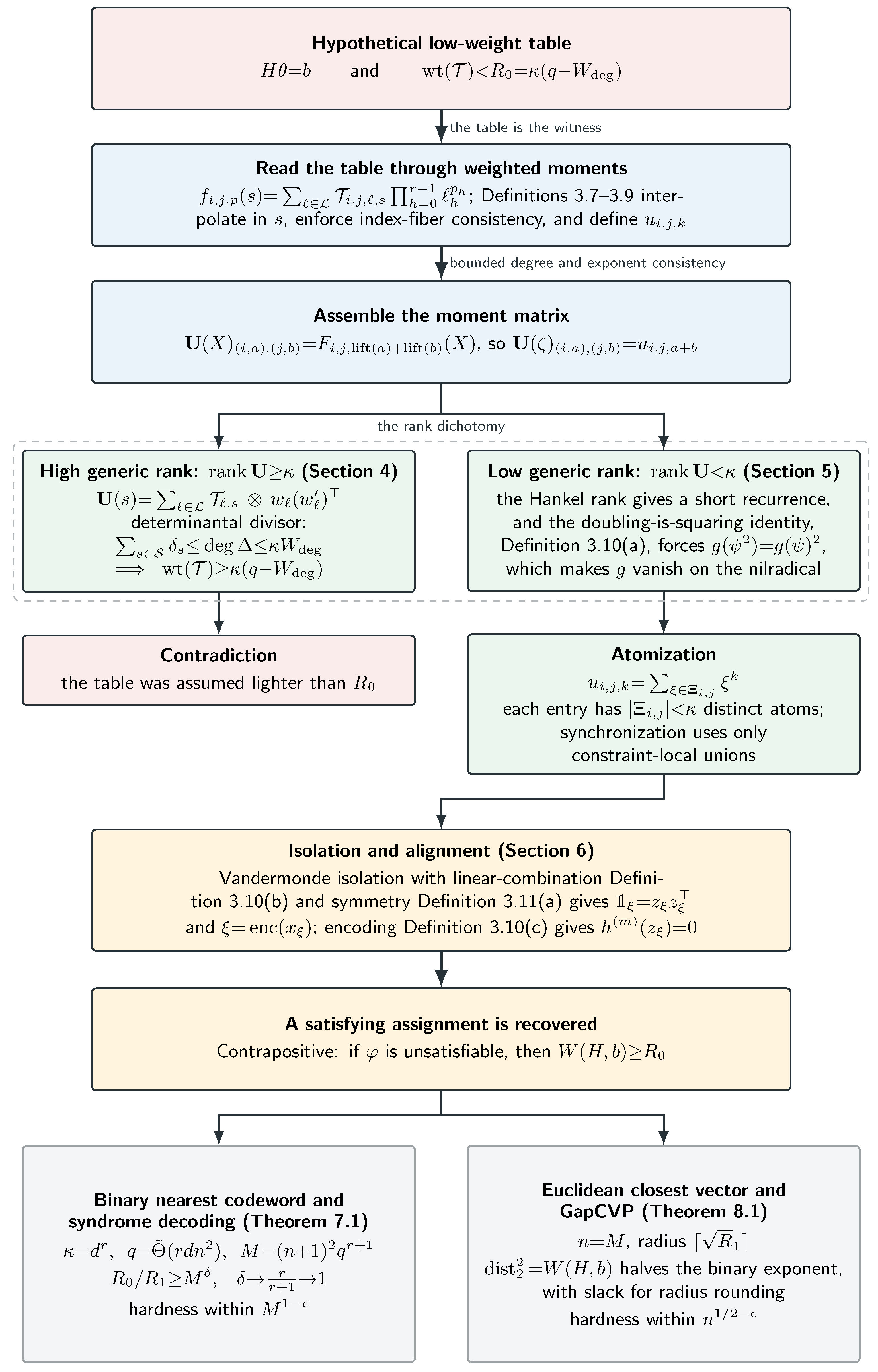
Figure 2.
A comparison of the bounded lift under two bases. With the same scalar , lift bound , and length , base gives and , whereas base gives and . The superscripts and subscripts record the base only for this comparison; in the construction, d is fixed and therefore suppressed from the notation.
Figure 2.
A comparison of the bounded lift under two bases. With the same scalar , lift bound , and length , base gives and , whereas base gives and . The superscripts and subscripts record the base only for this comparison; in the construction, d is fixed and therefore suppressed from the notation.
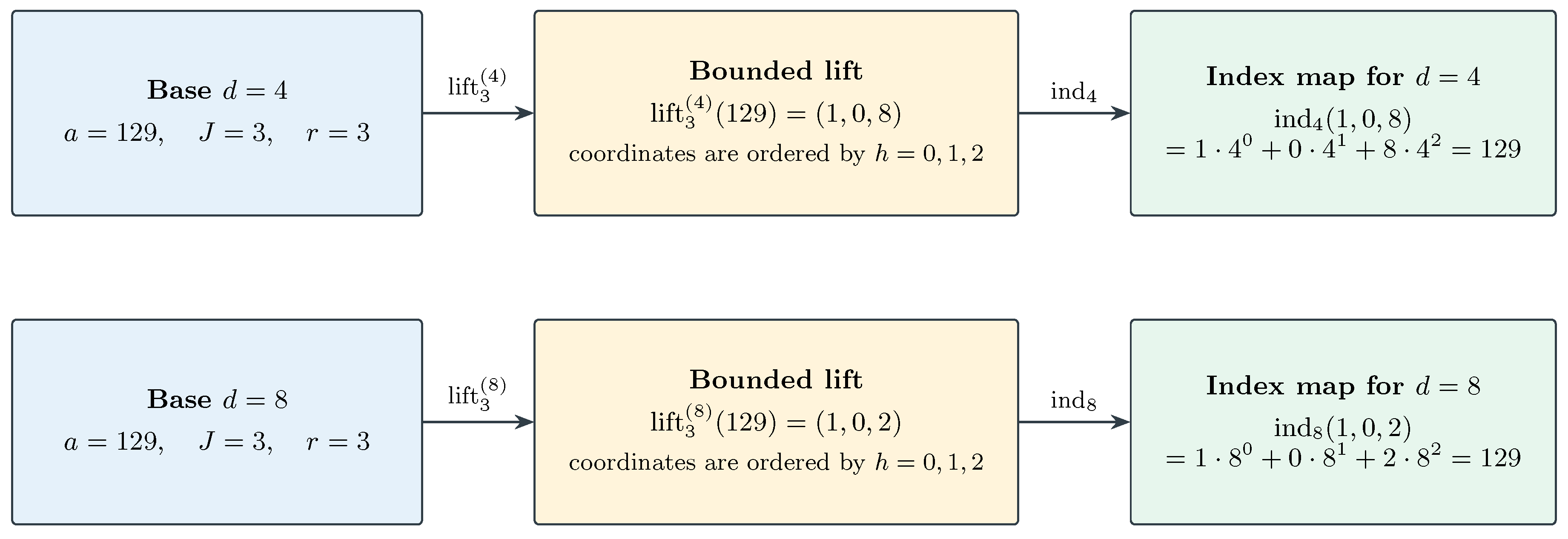
Figure 3.
Rank charging. The same deficit appears both as rank lost in the local weight bound and as the multiplicity of the zero of at s. The degree of therefore controls the total loss over all sample points.
Figure 3.
Rank charging. The same deficit appears both as rank lost in the local weight bound and as the multiplicity of the zero of at s. The degree of therefore controls the total loss over all sample points.
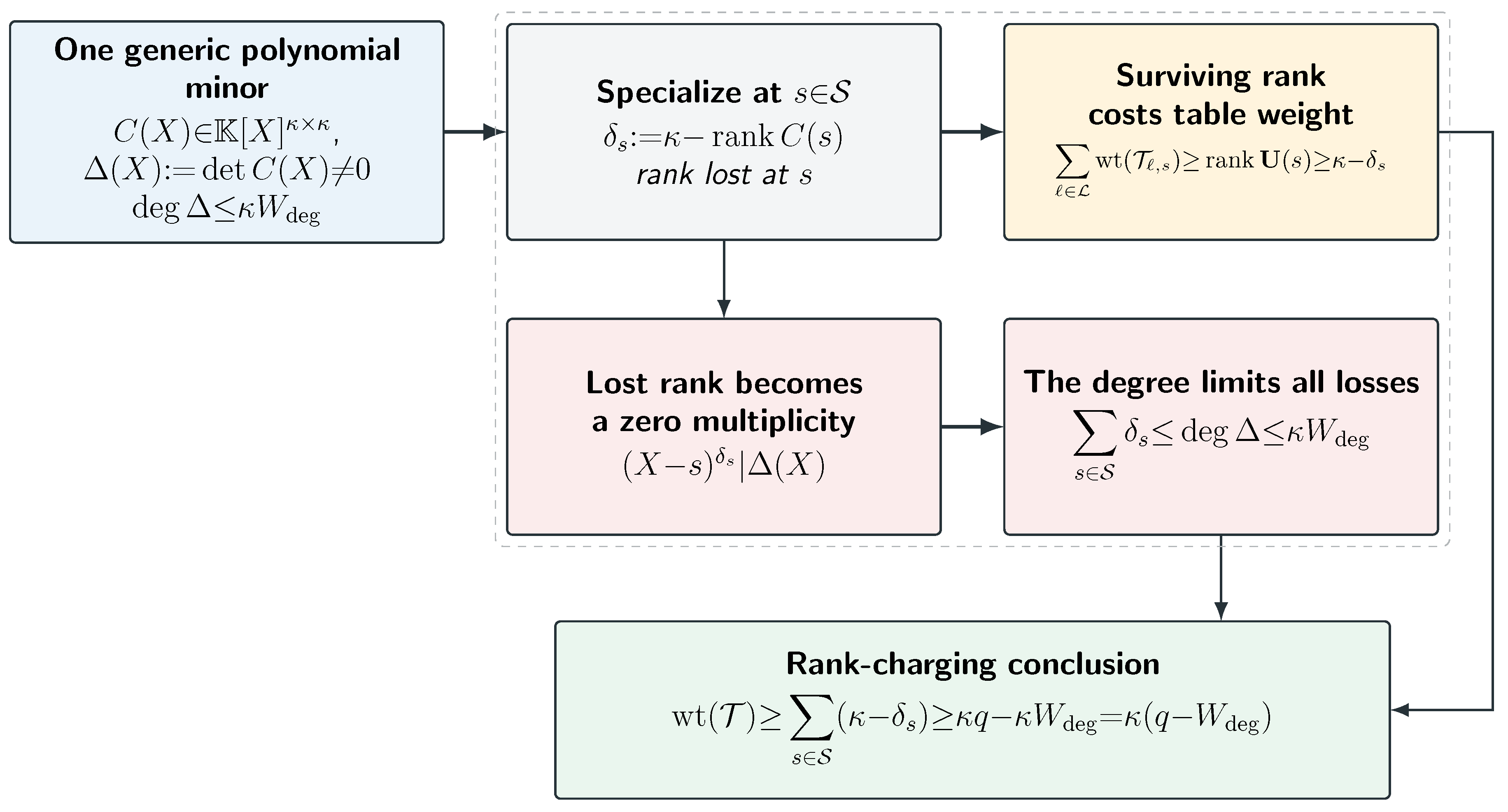
Figure 4.
Short-recurrence atomization for a fixed matrix entry. Low Hankel rank gives a short recurrence and candidate atoms. The doubling-is-squaring identity makes g vanish on nilpotents and forces every surviving coefficient to equal one, producing the entrywise set .
Figure 4.
Short-recurrence atomization for a fixed matrix entry. Low Hankel rank gives a short recurrence and candidate atoms. The doubling-is-squaring identity makes g vanish on nilpotents and forces every surviving coefficient to equal one, producing the entrywise set .
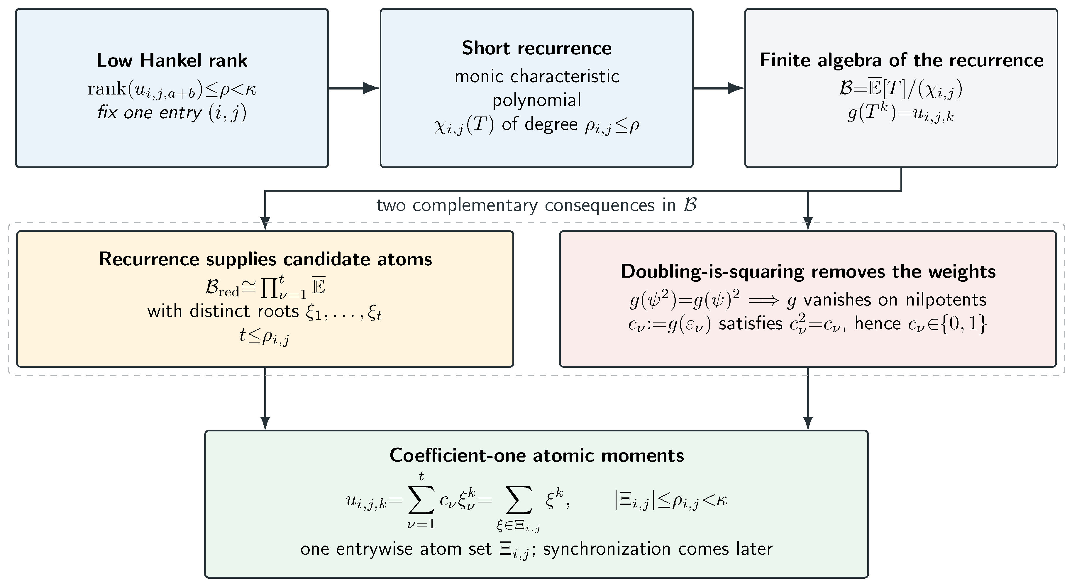
Figure 5.
Constraint-local synchronization. No bound is imposed on the global union of the entrywise atom sets. Instead, each constraint uses fewer than atoms, so Vandermonde isolation converts its moment identity into atomwise symmetry, linear-combination, encoding, or anchor conditions.
Figure 5.
Constraint-local synchronization. No bound is imposed on the global union of the entrywise atom sets. Instead, each constraint uses fewer than atoms, so Vandermonde isolation converts its moment identity into atomwise symmetry, linear-combination, encoding, or anchor conditions.
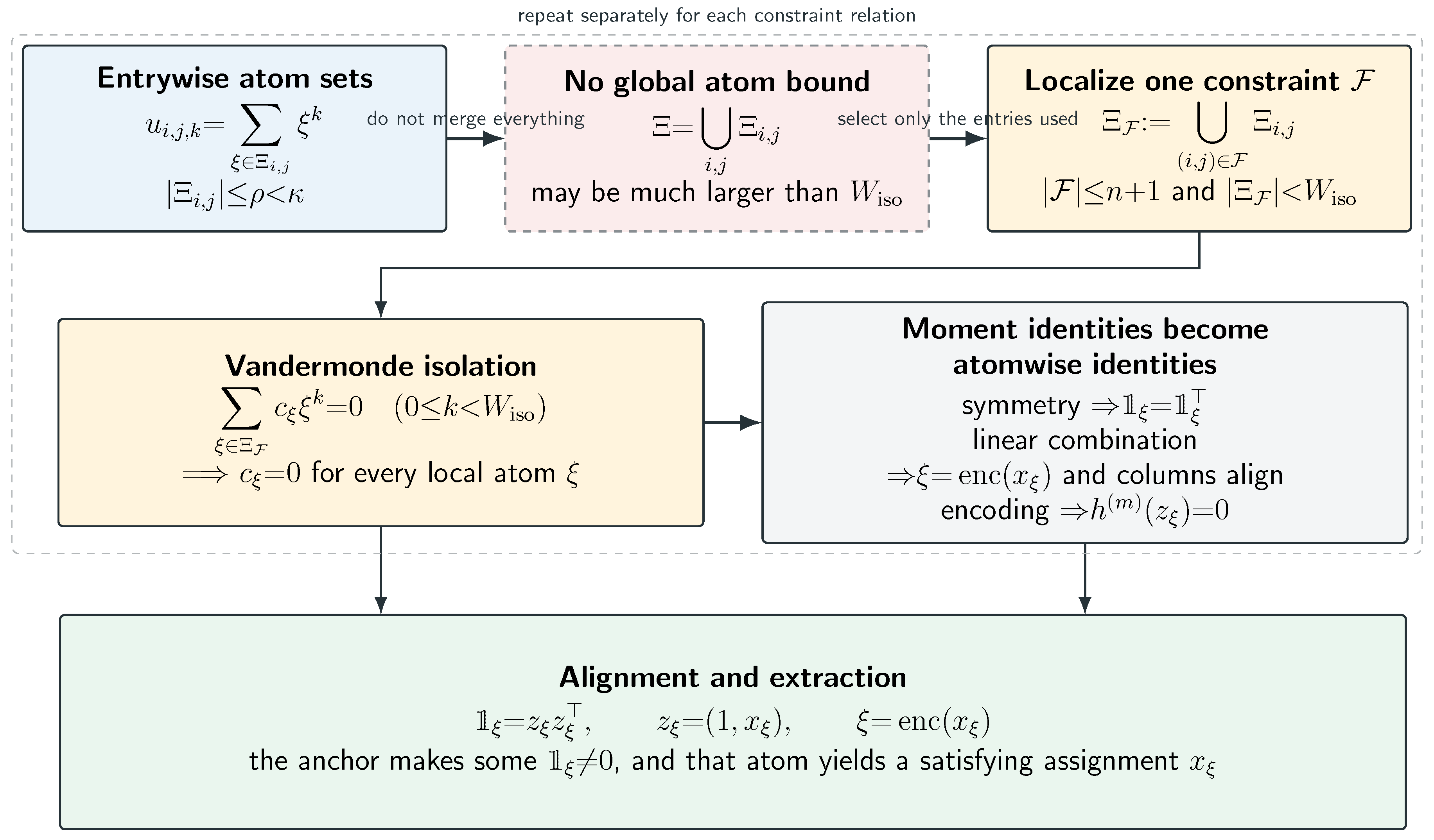

Table 1.
Historical hardness lower bounds and algorithmic upper bounds for Euclidean closest vector, measured as a function of the lattice rank n. In the second panel, D and R denote deterministic and randomized algorithms, respectively, and poly abbreviates polynomial time. In the 1997 row, the constant-factor hardness is unconditional, whereas the factor assumes . In the 2003 row, is an absolute constant. The final hardness row holds for every fixed .
Table 1.
Historical hardness lower bounds and algorithmic upper bounds for Euclidean closest vector, measured as a function of the lattice rank n. In the second panel, D and R denote deterministic and randomized algorithms, respectively, and poly abbreviates polynomial time. In the 1997 row, the constant-factor hardness is unconditional, whereas the factor assumes . In the 2003 row, is an absolute constant. The final hardness row holds for every fixed .
| Year | Authors | Reference | Ratio |
|---|---|---|---|
| 1997 | Arora, Babai, Stern, and Sweedyk | [ABSS97] | Every constant; |
| 2003 | Dinur, Kindler, Raz, and Safra | [DKRS03] | |
| 2026 | OpenAI | [Ope26] | |
| 2026 | This paper | Theorem 1.3 |
Table 2.
Historical hardness lower bounds and algorithmic upper bounds for binary nearest codeword. In the first panel, the 2005 and 2014 rows concern nearest codeword with preprocessing; all other rows concern ordinary nearest codeword or the equivalent syndrome-decoding formulation. The constant-factor statements in the 1997 and 2025 rows are unconditional. The statements in those rows, as well as the 2005 row, assume ; the 2014 row assumes . Both 2026 hardness results are unconditional, and the final row holds for every fixed . In the second panel, n denotes the binary block length, k denotes the code dimension, and R and D denote randomized and deterministic algorithms, respectively. The randomized 2002 row records the sharper guarantee that Alon, Panigrahy, and Yekhanin observed from Berman and Karpinski’s analysis; Berman and Karpinski themselves stated . In the first row of the second panel, is an arbitrary fixed constant. The parameter s is a fixed positive integer, and denotes the s-fold iterated logarithm.
Table 2.
Historical hardness lower bounds and algorithmic upper bounds for binary nearest codeword. In the first panel, the 2005 and 2014 rows concern nearest codeword with preprocessing; all other rows concern ordinary nearest codeword or the equivalent syndrome-decoding formulation. The constant-factor statements in the 1997 and 2025 rows are unconditional. The statements in those rows, as well as the 2005 row, assume ; the 2014 row assumes . Both 2026 hardness results are unconditional, and the final row holds for every fixed . In the second panel, n denotes the binary block length, k denotes the code dimension, and R and D denote randomized and deterministic algorithms, respectively. The randomized 2002 row records the sharper guarantee that Alon, Panigrahy, and Yekhanin observed from Berman and Karpinski’s analysis; Berman and Karpinski themselves stated . In the first row of the second panel, is an arbitrary fixed constant. The parameter s is a fixed positive integer, and denotes the s-fold iterated logarithm.
| Year | Authors | Reference | Ratio |
|---|---|---|---|
| 1997 | Arora, Babai, Stern, and Sweedyk | [ABSS97] | Every constant; |
| 2005 | Alekhnovich, Khot, Kindler, and Vishnoi | [3] | |
| 2014 | Khot, Popat, and Vishnoi | [KPV14] | |
| 2025 | Bhattiprolu, Guruswami, and Ren | [BGR25] | Every constant; |
| 2026 | OpenAI | [Ope26] | |
| 2026 | This paper | Theorem 1.8 |
Disclaimer/Publisher’s Note: The statements, opinions and data contained in all publications are solely those of the individual author(s) and contributor(s) and not of MDPI and/or the editor(s). MDPI and/or the editor(s) disclaim responsibility for any injury to people or property resulting from any ideas, methods, instructions or products referred to in the content. |
© 2026 by the authors. Licensee MDPI, Basel, Switzerland. This article is an open access article distributed under the terms and conditions of the Creative Commons Attribution (CC BY) license (http://creativecommons.org/licenses/by/4.0/).
Copyright: This open access article is published under a Creative Commons CC BY 4.0 license, which permit the free download, distribution, and reuse, provided that the author and preprint are cited in any reuse.