Hardness of Euclidean Closest Vector Within n^1/8−ϵ and Binary Nearest Codeword Within n^1/4−ϵ

1. Introduction

The gap version of the closest vector problem provides the standard decision formulation for studying approximation hardness. Let $B\in {\mathbb{Z}}^{n\times n}$ be nonsingular. Its columns generate the full-rank lattice $\mathcal{L}\left(B\right):=B{\mathbb{Z}}^n$, whose rank is n. Given a target $t\in {\mathbb{Q}}^n$ and a norm $\parallel ·\parallel$, the optimization version of the closest vector problem asks for $z\in {\mathbb{Z}}^n$ minimizing $\parallel t-Bz\parallel$; see Micciancio and Goldwasser [2][Chapter 3] for standard background.

For an approximation factor $\gamma :\mathbb{N}\to [1,\infty )$ and a positive rational radius r, the promise problem ${GapCVP}_{\gamma }^{\parallel ·\parallel }$ asks one to distinguish

$${dist}_{\parallel ·\parallel }(t,\mathcal{L}\left(B\right))\le r\mathrm{from}{dist}_{\parallel ·\parallel }(t,\mathcal{L}\left(B\right))>\gamma \left(n\right)r,$$

where ${dist}_{\parallel ·\parallel }(t,\mathcal{L}\left(B\right)):={min}_{z\in {\mathbb{Z}}^n}\parallel t-Bz\parallel$. Instances whose optimum lies between the two thresholds are outside the promise. A $\gamma \left(n\right)$-approximation algorithm for the optimization problem solves this promise problem by comparing the distance of its output with $\gamma \left(n\right)r$. Thus NP-hardness of ${GapCVP}_{\gamma }^{\parallel ·\parallel }$ rules out such an approximation algorithm unless $\mathrm{P}=\mathrm{NP}$.

The Euclidean closest vector problem is the specialization to the ${\ell }_2$ norm. We write

$${dist}_2(t,\mathcal{L}\left(B\right)):=\underset{z\in {\mathbb{Z}}^n}{min}{\parallel t-Bz\parallel }_2$$

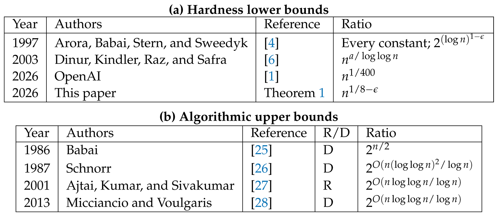
and denote its gap version by ${GapCVP}_{\gamma }^{\left(2\right)}$. Van Emde Boas [3] proved NP-hardness of exact Euclidean CVP. Arora, Babai, Stern, and Sweedyk [4] established hardness within every fixed constant. For every fixed $ϵ>0$, they also proved hardness within $2^{{(logn)}^{1-ϵ}}$ under the assumption $\mathrm{NP}\neg \subseteq \mathrm{DTIME}\left(2^{{(logn)}^{O\left(1\right)}}\right)$ [4]. Dinur, Kindler, and Safra [5], in work subsequently refined by Dinur, Kindler, Raz, and Safra [6], strengthened this to $n^{a/loglogn}$ for some absolute constant $a>0$. Although this factor dominates every fixed power of $logn$, its exponent tends to zero and hence does not give $n^c$ hardness for any fixed $c>0$. The OpenAI report [1][Chapter 7] subsequently obtained the fixed polynomial factor $n^{1/400}$ by a deterministic reduction from 3SAT. Fixed-polynomial lattice inapproximability had previously been obtained conditionally on the Projection Games Conjecture by Moshkovitz [7][Section 5.1] and Mukhopadhyay [8]. Those conditional results are qualitatively different from the unconditional deterministic reduction from ordinary 3SAT proved here. The Exponential Time Hypothesis (ETH), introduced by Impagliazzo and Paturi [9], has also served as the basis for recent fine-grained lower bounds for constant-factor approximations of CVP and related problems [10,11]. These results concern the running time of constant-factor approximation rather than unconditional NP-hardness for polynomial approximation factors.

The square-root scale forms a complexity-theoretic barrier. Goldreich and Goldwasser [12] established interactive-proof upper bounds that constrain the nonapproximability of lattice problems. Aharonov and Regev [13] subsequently proved that, for some absolute constant $C>0$,

$${GapCVP}_{C\sqrt{n}}^{\left(2\right)}\in \mathrm{NP}\cap \mathrm{coNP}.$$

Consequently, NP-hardness at that scale under deterministic polynomial-time many-one reductions would imply $\mathrm{NP}=\mathrm{coNP}$. The range between the exponent $1/8$ obtained here and the square-root exponent $1/2$ remains open.

Binary nearest codeword is an optimization problem over ${\mathbb{F}}_2$. Given a k-dimensional binary linear code $C\subseteq {\mathbb{F}}_2^n$ and a target word $y\in {\mathbb{F}}_2^n$, the task is to find a codeword in C minimizing its Hamming distance from y [14]. Binary syndrome decoding takes as input a binary parity-check matrix H and a syndrome $s\in imH$, and asks for a minimum-weight binary vector e satisfying $He=s$ [14]. The two formulations are equivalent. Indeed, if $C=kerH$ and $s=Hy$, then the map $c\mapsto y-c$ identifies codewords $c\in C$ with vectors e satisfying $He=s$. Consequently, the two instances have the same optimum value, and the correspondence preserves approximation ratios.

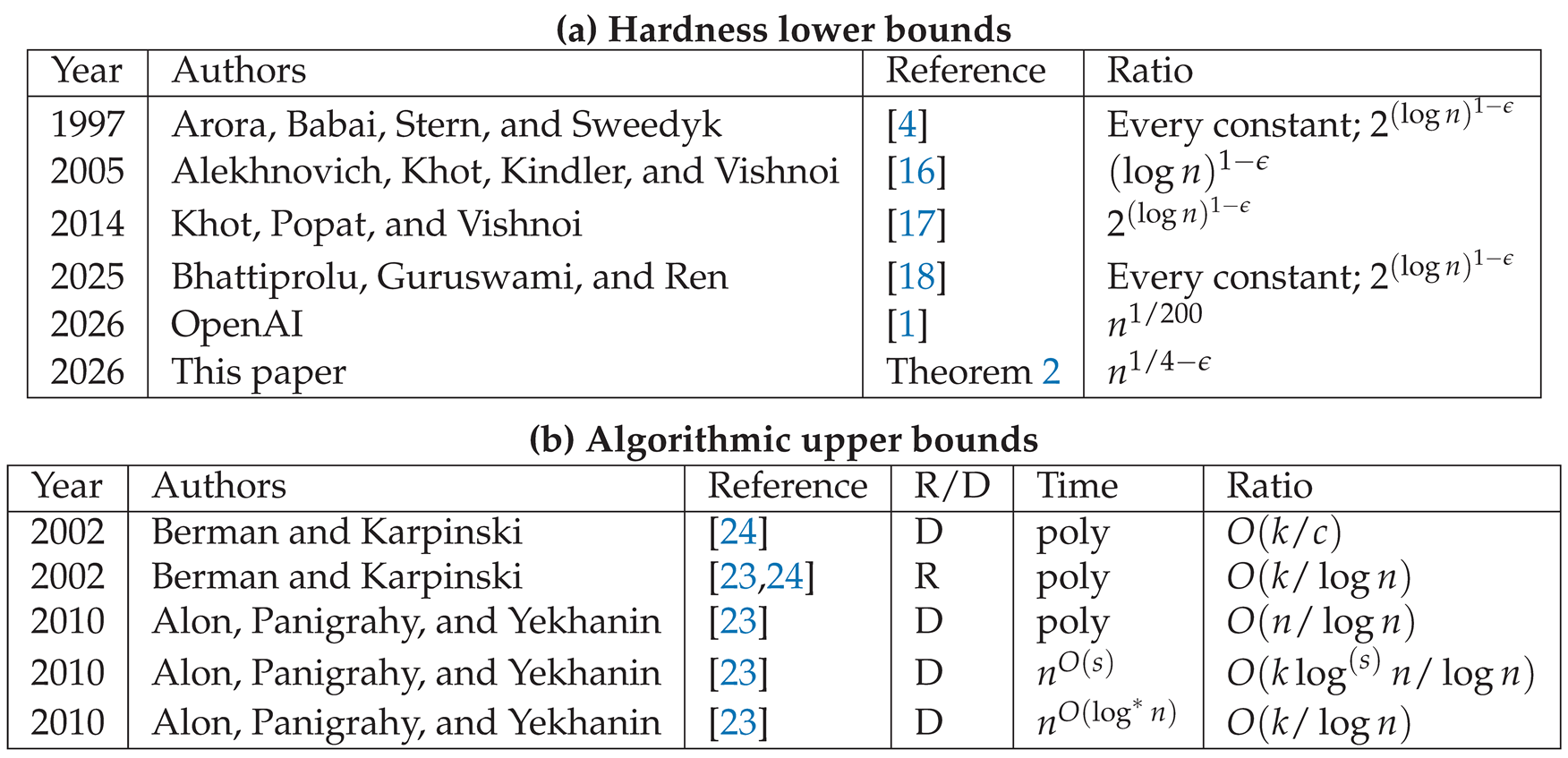
Berlekamp, McEliece, and van Tilborg [14] proved that binary syndrome decoding is NP-complete. For binary nearest codeword, Arora, Babai, Stern, and Sweedyk [4] proved unconditional NP-hardness of approximation within every constant factor. For every fixed $ϵ>0$, they also proved hardness within $2^{{(logn)}^{1-ϵ}}$ under the assumption that NP has no quasipolynomial-time algorithms, namely $\mathrm{NP}\neg \subseteq \mathrm{DTIME}\left(2^{{(logn)}^{O\left(1\right)}}\right)$. Arora’s thesis [15][Section 6.4] gives a contemporaneous account and explicitly records the stronger $1-ϵ$ exponent for nearest codeword. For nearest codeword with preprocessing, Alekhnovich, Khot, Kindler, and Vishnoi [16] proved hardness within ${(logn)}^{1-ϵ}$ under the same quasipolynomial-time assumption. Khot, Popat, and Vishnoi [17] strengthened the factor to $2^{{(logn)}^{1-ϵ}}$ under $\mathrm{NP}\neg \subseteq \mathrm{DTIME}\left(2^{{(logn)}^{O(1/ϵ)}}\right)$. For ordinary nearest codeword, Bhattiprolu, Guruswami, and Ren [18] subsequently gave a PCP-free proof of the same two bounds: unconditional NP-hardness within every constant factor and $2^{{(logn)}^{1-ϵ}}=n^{o\left(1\right)}$ hardness under the assumption that NP has no quasipolynomial-time algorithms. Their contribution is a new proof rather than a stronger approximation factor. Bhattiprolu, Guruswami, Lee, and Ren [19] subsequently studied the inapproximability of finding sparse vectors in codes, subspaces, and lattices via randomized reductions; their lattice result does not yield deterministic fixed-polynomial hardness for Euclidean CVP. Methodologically, Bennett and Peikert [20] also combine Reed–Solomon codes [21] with an integer-lattice lift to obtain randomized hardness for approximate SVP and identify derandomization as a central obstacle.

Bitansky, Harsha, Ishai, Rothblum, and Wu [22] showed that ETH rules out $2^{o\left(n\right)}$-time approximation within a certain constant factor, using the equivalent formulation that minimizes the number of unsatisfied linear equations. Subsequently, Corollary 15 of the OpenAI report [1] established, without an additional complexity assumption, NP-hardness of approximation within $n^{1/200}$ for binary nearest codeword and binary syndrome decoding under deterministic polynomial-time many-one reductions. The result proved here uses the same unconditional reduction model and improves the approximation factor to $n^{1/4-ϵ}$ for every fixed $ϵ>0$.

On the algorithmic side, Alon, Panigrahy, and Yekhanin gave several deterministic approximation algorithms and time–ratio tradeoffs [23]. Their general polynomial-time algorithm achieves an $O(n/logn)$ approximation. Berman and Karpinski gave a deterministic $O(k/c)$-approximation algorithm for every fixed constant $c>0$ and a randomized $O(k/logk)$-approximation algorithm [24]. Alon, Panigrahy, and Yekhanin observed that the latter analysis yields an $O(k/logn)$ approximation [23].

1.1. Our Results

We first record the two Euclidean lattice problems used below.

Definition 1

(Euclidean closest vector). An instance consists of a nonsingular matrix $B\in {\mathbb{Z}}^{n\times n}$ and a target $t\in {\mathbb{Q}}^n$. The matrix B generates the full-rank lattice $\mathcal{L}\left(B\right):=B{\mathbb{Z}}^n$. The objective is to output a vector $z\in {\mathbb{Z}}^n$ minimizing ${\parallel t-Bz\parallel }_2$. Its optimum value is ${dist}_2(t,\mathcal{L}\left(B\right)):={min}_{z\in {\mathbb{Z}}^n}{\parallel t-Bz\parallel }_2$.

Definition 2

(Euclidean GapCVP). Let $\gamma :\mathbb{N}\to [1,\infty )$. An instance of ${GapCVP}_{\gamma }^{\left(2\right)}$ consists of a nonsingular matrix $B\in {\mathbb{Z}}^{n\times n}$, a target $t\in {\mathbb{Q}}^n$, and a radius $r\in {\mathbb{Q}}_{>0}$. It is promised that either ${dist}_2(t,\mathcal{L}\left(B\right))\le r$, which is the YES case, or ${dist}_2(t,\mathcal{L}\left(B\right))>\gamma \left(n\right)r$, which is the NO case. The task is to distinguish the two cases.

We now state our main Euclidean result. It improves the $n^{1/400}$ hardness factor in Theorem 1 on page 184 of the OpenAI report [1][Chapter 7].

Theorem 1

(Euclidean closest vector, informal version of Theorem 4). For every fixed $ϵ>0$, there is a deterministic polynomial-time mapping that assigns to each 3SAT formula φ a nonsingular matrix $B\in {\mathbb{Z}}^{n\times n}$, a target $t\in {\mathbb{Z}}^n$, and a radius $r\in {\mathbb{Q}}_{>0}$ such that

$$\begin{array}{cc}\hfill \phi \mathrm{satisfiable}& \Rightarrow {dist}_2(t,\mathcal{L}\left(B\right))\le r,\hfill \\ \hfill \phi \mathrm{unsatisfiable}& \Rightarrow {dist}_2(t,\mathcal{L}\left(B\right))>n^{1/8-ϵ}r.\hfill \end{array}$$

Consequently, ${GapCVP}_{n^{1/8-ϵ}}^{\left(2\right)}$ is NP-hard under deterministic polynomial-time many-one reductions.

We next formally define the two binary problems.

Definition 3

(Binary nearest codeword). An instance consists of a binary linear code $C\subseteq {\mathbb{F}}_2^n$, given by a generator matrix, and a target word $y\in {\mathbb{F}}_2^n$. The objective is to output a codeword $c\in C$ minimizing $wt(y-c)$. We denote the optimum value by ${opt}_{\mathrm{nc}}(C,y):={min}_{c\in C}wt(y-c).$

Definition 4

(Binary syndrome decoding). An instance consists of a binary matrix $H\in {\mathbb{F}}_2^{r\times n}$ and a syndrome $s\in imH$. The objective is to output a vector $e\in {\mathbb{F}}_2^n$ of minimum Hamming weight subject to $He=s$. We denote the optimum value by ${opt}_{\mathrm{sd}}(H,s):=min\{wt\left(e\right):e\in {\mathbb{F}}_2^n,He=s\}.$

The following theorem improves the $n^{1/200}$ hardness factor established by Corollary 15 on page 213 of the OpenAI report [1][Chapter 7].

Theorem 2

(Main result, informal version of Theorem 3). For every $ϵ>0$, binary nearest codeword (Definition 3) and binary syndrome decoding (Definition 4) are NP-hard to approximate within $n^{1/4-ϵ}$ under deterministic polynomial-time many-one reductions, where n is the binary block length.

2. Technique Overview

This section compares the mechanism behind the OpenAI reduction with the two quadratic estimates that improve its parameters. We focus on the reduction to binary nearest codeword and syndrome decoding. The Euclidean closest-vector result then follows from the dimension-preserving parity-lift reduction, which takes a binary weight gap to the square root of that gap in Euclidean distance.

Table 1. Historical hardness lower bounds and algorithmic upper bounds for Euclidean closest vector, measured as a function of the lattice rank n. Every algorithm in the second panel runs in polynomial time; D and R denote deterministic and randomized algorithms, respectively. In the 1997 row, the constant-factor hardness is unconditional, whereas the $2^{{(logn)}^{1-ϵ}}$ factor assumes $\mathrm{NP}\neg \subseteq \mathrm{DTIME}\left(2^{{(logn)}^{O\left(1\right)}}\right)$. In the 2003 row, $a>0$ is an absolute constant. The final hardness row holds for every fixed $ϵ>0$.

Table 1. Historical hardness lower bounds and algorithmic upper bounds for Euclidean closest vector, measured as a function of the lattice rank n. Every algorithm in the second panel runs in polynomial time; D and R denote deterministic and randomized algorithms, respectively. In the 1997 row, the constant-factor hardness is unconditional, whereas the $2^{{(logn)}^{1-ϵ}}$ factor assumes $\mathrm{NP}\neg \subseteq \mathrm{DTIME}\left(2^{{(logn)}^{O\left(1\right)}}\right)$. In the 2003 row, $a>0$ is an absolute constant. The final hardness row holds for every fixed $ϵ>0$.

2.1. Overview of the OpenAI Reduction

Chapter 7 of the OpenAI report factors the reduction as

$$3\mathrm{SAT}⟶\mathrm{binary}\mathrm{affine}\mathrm{decoding}⟶\mathrm{binary}\mathrm{nearest}\mathrm{codeword}⟶\mathrm{Euclidean}\mathrm{CVP};$$

see [1][Section 1.2]. The first arrow contains the main algebraic construction. Let $\phi$ be the input formula, let s be its encoding length, and let m and ℓ be its numbers of variables and clauses. Put $N:=100+s+m+\ell$ and $d:=m$. The variables are indexed by $\left[m\right]:=\{1,\dots ,m\}$ and represented by distinct anchors $a_1,\dots ,a_m$ in a characteristic-two field ${\mathbb{F}}_q$. A Boolean assignment $\sigma \in {\{0,1\}}^m$ determines the unique polynomial $Q_{\sigma }\in {\mathbb{F}}_q\left[X\right]$ of degree less than m satisfying $Q_{\sigma }\left(a_i\right)={\sigma }_i$, where ${\sigma }_i$ is the bit assigned to variable i. The reduction evaluates this polynomial on $P:={\mathbb{F}}_q\setminus \{a_1,\dots ,a_m\}$.

The binary variables are arranged into evaluation tables. For a clause C, let $I_C\subseteq \left[m\right]$ be the set of its variable indices and let $B_C\subseteq {\{0,1\}}^{I_C}$ be its satisfying local assignments. The table types are $\Theta :=\left\{0\right\}\cup \{(C,\beta ):\beta \in B_C\}$: type 0 is the global table, and $(C,\beta )$ is the subtype asserting that clause C receives the local assignment $\beta$. Write $x_{\tau ,p,w}$ for the binary coordinate selecting the field value $w\in {\mathbb{F}}_q$ in table $\tau \in \Theta$ at $p\in P$, and define its fiber by $S_{\tau }\left(p\right):=\{w\in {\mathbb{F}}_q:x_{\tau ,p,w}=1\}$.

Fix a moment budget T. For $0\le j\le T$, the ordinary power sum of table $\tau$ at p is

$${\mu }_{\tau ,j}\left(p\right):=\sum _{w\in S_{\tau }\left(p\right)}{w}^j.$$

For $\tau =(C,\beta )$, $i\in I_C$, and $0\le j\le T$, the shifted power sum is

$${\eta }_{\tau ,i,j}\left(p\right):=\sum _{w\in S_{\tau }\left(p\right)}{\left({\displaystyle \frac{w-{\beta }_i}{p-a_i}}\right)}^j,$$

where ${\beta }_i$ is the bit assigned to variable i by $\beta$. The affine constraints require these pointwise quantities to be evaluations of low-degree polynomials and require the clause tables to reproduce the global table modulo two. Let $Hx=b$ denote the resulting binary affine system, let $M:=\left|\Theta \right|\left|P\right|q$ be its number of binary coordinates, and, when the system is consistent, define $W(H,b):=min\{wt(x):Hx=b\}.$ If $\sigma$ satisfies the formula, each active fiber is the singleton $\left\{Q_{\sigma }\left(p\right)\right\}$, exactly one subtype is active for every clause, and the resulting binary solution has weight $R:=(\ell +1)\left|P\right|$.

For soundness, start with a low-weight binary solution. For a fiber cutoff $\kappa$, define the good evaluation set of table $\tau$ by $P_{\tau }:=\{p\in P:|S_{\tau }\left(p\right)|\le \kappa \}$. Markov’s inequality shows that $P_{\tau }$ contains all but a small set of evaluation points. Reed–Solomon interpolation turns the pointwise moments into polynomials ${\mu }_{\tau ,j}\left(X\right)$ in the indeterminate X. The report’s reconstruction lemma uses the associated Hankel matrix to construct a monic separable polynomial $G_{\tau }\in {\mathbb{F}}_q\left(X\right)\left[Y\right]$. Its roots in a common splitting field have the prescribed power sums. The shifted moments are then examined using a valuation above $X-a_i$. They force every root associated with subtype $(C,\beta )$ to reduce to the bit ${\beta }_i$ at the anchor $a_i$. Finally, the clause decomposition and a Vandermonde argument match a global root with a satisfying subtype for every clause. Using the same valuation for a variable wherever it occurs makes these local assignments consistent, producing a global satisfying assignment.

Table 2. Historical hardness lower bounds and algorithmic upper bounds for binary nearest codeword. In the first panel, the 2005 and 2014 rows concern nearest codeword with preprocessing; all other rows concern ordinary nearest codeword or the equivalent syndrome-decoding formulation. The constant-factor statements in the 1997 and 2025 rows are unconditional. The $2^{{(logn)}^{1-ϵ}}$ statements in those rows, as well as the 2005 row, assume $\mathrm{NP}\neg \subseteq \mathrm{DTIME}\left(2^{{(logn)}^{O\left(1\right)}}\right)$; the 2014 row assumes $\mathrm{NP}\neg \subseteq \mathrm{DTIME}\left(2^{{(logn)}^{O(1/ϵ)}}\right)$. Both 2026 hardness results are unconditional, and the final row holds for every fixed $ϵ>0$. In the second panel, n denotes the binary block length, k denotes the code dimension, and R and D denote randomized and deterministic algorithms, respectively. The randomized 2002 row records the sharper $O(k/logn)$ guarantee that Alon, Panigrahy, and Yekhanin observed from Berman and Karpinski’s analysis; Berman and Karpinski themselves stated $O(k/logk)$. In the first row of the second panel, $c>0$ is an arbitrary fixed constant. The parameter s is a fixed positive integer, and ${log}^{\left(s\right)}n$ denotes the s-fold iterated logarithm.

Table 2. Historical hardness lower bounds and algorithmic upper bounds for binary nearest codeword. In the first panel, the 2005 and 2014 rows concern nearest codeword with preprocessing; all other rows concern ordinary nearest codeword or the equivalent syndrome-decoding formulation. The constant-factor statements in the 1997 and 2025 rows are unconditional. The $2^{{(logn)}^{1-ϵ}}$ statements in those rows, as well as the 2005 row, assume $\mathrm{NP}\neg \subseteq \mathrm{DTIME}\left(2^{{(logn)}^{O\left(1\right)}}\right)$; the 2014 row assumes $\mathrm{NP}\neg \subseteq \mathrm{DTIME}\left(2^{{(logn)}^{O(1/ϵ)}}\right)$. Both 2026 hardness results are unconditional, and the final row holds for every fixed $ϵ>0$. In the second panel, n denotes the binary block length, k denotes the code dimension, and R and D denote randomized and deterministic algorithms, respectively. The randomized 2002 row records the sharper $O(k/logn)$ guarantee that Alon, Panigrahy, and Yekhanin observed from Berman and Karpinski’s analysis; Berman and Karpinski themselves stated $O(k/logk)$. In the first row of the second panel, $c>0$ is an arbitrary fixed constant. The parameter s is a fixed positive integer, and ${log}^{\left(s\right)}n$ denotes the s-fold iterated logarithm.

The quantitative loss comes from making the reconstruction and valuation arguments hold simultaneously. The report chooses $\kappa :=N^4$, $T:=N^{30}$, and $q=\Theta \left(N^{200}\right)$. Since the number of binary coordinates is $M=O\left(N{q}^2\right)=O\left(N^{401}\right)$, soundness against solutions of weight $O\left(M^{1/200}R\right)$ gives the $M^{1/200}$ coding gap. The standard parity lift outputs a lattice basis B and a target t satisfying ${dist}_2{(t,\mathcal{L}\left(B\right))}^2=W(H,b)$, so this becomes the $M^{1/400}$ Euclidean gap.

2.2. Overview of Our Improvements

Our construction retains the evaluation tables, the ordinary and shifted Reed–Solomon moment constraints, and the completeness assignment above. The improvement comes from replacing the two most expensive parts of the soundness analysis by quadratic estimates in the fiber cutoff $\kappa$.

The first improvement is Lemma 2. Fix a table type $\tau$ and a set $P^{\prime }\subseteq P_{\tau }$ of good evaluation points. For readability, write ${\mu }_j\left(X\right):={\mu }_{\tau ,j}\left(X\right)$. Let $h:={max}_{p\in P^{\prime }}\left|S_{\tau }\left(p\right)\right|$ be the maximum fiber size on $P^{\prime }$, and form the Hankel determinant

$${\Delta }_h\left(X\right):=det{\left({\mu }_{r+s}\left(X\right)\right)}_{0\le r,s<h}.$$

At a fiber of size h this determinant is a squared Vandermonde determinant, whereas it vanishes at smaller fibers. Expanding the determinant and using $deg{\mu }_{r+s}\le d(r+s)$ gives $deg{\Delta }_h\le dh(h-1)$. Solving the Hankel system gives a recurrence for the moments and a monic polynomial $G\in {\mathbb{F}}_q\left(X\right)\left[Y\right]$. Instead of propagating the recurrence one moment at a time with a fresh denominator loss, we package it into the generating-function identity

$$Q\left(Z\right)U_T\left(Z\right)=hQ\left(Z\right)-Z{Q}^{\prime }\left(Z\right)(mod{Z}^{T+1}),$$

where Z is a formal variable, $Q\left(Z\right):=Z^{h}G\left(Z^{-1}\right)$, and $U_T\left(Z\right):={\sum }_{j=0}^T{\mu }_j\left(X\right)Z^j$. Only one copy of the Hankel denominator must be cleared. This changes the sampling requirement from the report’s product-type bound $2d{\kappa }^{2}T$ to the additive quadratic bound

$$|P^{\prime }|-d\kappa (\kappa -1)>d(T+{\kappa }^2).$$

It also recovers all moments through T and proves that G is separable.

The second improvement is Lemma 3. Fix an anchor $a_i$, a subtype bit ${\beta }_i$, and reconstructed roots ${\alpha }_1,\dots ,{\alpha }_h$ in a splitting field of G. Let v be an extension to this field of the $(X-a_i)$-adic valuation ${ord}_{X-a_i}$. Put $y_s:=({\alpha }_s-{\beta }_i)/(X-a_i)$. The shifted constraints say that the power sums of the $y_s$ have nonnegative v-valuation. Suppose, for contradiction, that some $y_s$ has negative valuation, and collect all roots of minimum valuation into one cluster. A Newton-polygon segment shows that the cluster size times the absolute slope is at least one. A logarithmic-derivative identity bounds the derivatives at the reciprocal roots, while the discriminant identity

$${\Delta }_h=\prod _{r<s}{({\alpha }_s-{\alpha }_r)}^2$$

bounds the total pairwise valuation. Summing over the entire minimum-slope cluster prevents cancellation among individual roots and yields a contradiction once $T\ge d{\kappa }^2$. Thus every reconstructed root satisfies $v({\alpha }_s-{\beta }_i)\ge 1$. The parity-matching argument can then be reused to obtain Lemma 4.

These quadratic bounds permit a substantially smaller field. Fix an integer tuning parameter $k\ge 2$, independent of the code dimension, and choose a constant A depending only on k. Define $\kappa :=A{N}^k$, $T:=N{\kappa }^2$, $q:=\Theta \left(N^2{\kappa }^2\right).$ The affine system then has $M=O_k\left(N{q}^2\right)=O_k\left(N^{4k+5}\right)$ coordinates, where the hidden constants depend only on k. Its binary block length is $n:=M$. Taking ${\delta }_k:=(k-1)/(4k+5)$ makes the low-weight cutoff $M^{{\delta }_k}R$ small enough that every table retains the evaluations needed by the two quadratic lemmas. Therefore an unsatisfiable formula has binary distance greater than $M^{{\delta }_k}R$, proving Theorem 3. Since ${\delta }_k$ tends to $1/4$, this gives $n^{1/4-ϵ}$ hardness for binary nearest codeword and syndrome decoding. After the parity lift, the resulting lattice has rank $n:=M$, and the Euclidean exponent is halved, giving the $n^{1/8-ϵ}$ consequence stated in Theorem 4.

3. The Binary Affine System

Let $\phi$ be a 3SAT formula of encoding length s. Delete tautological clauses, repeated literals, and unused variables. The cases of an empty clause and of no remaining clauses will be handled by fixed promise instances. Otherwise let $m,\ell \ge 1$ be the numbers of variables and clauses, and put

$$N:=100+s+m+\ell ,d:=m.$$

Let $\mathbb{K}:={\mathbb{F}}_q$ be a characteristic-two field, choose distinct anchors $a_1,\dots ,a_m\in \mathbb{K}$, and define

$$P:=\mathbb{K}\setminus \{a_1,\dots ,a_m\}.$$

For a clause C, let $I_C$ be its set of variable indices and let $B_C\subseteq {\{0,1\}}^{I_C}$ be the satisfying local assignments. Thus $|I_C|\le 3$ and $|B_C|\le 8$. The table types are

$$\Theta :=\left\{0\right\}\cup \{(C,\beta ):\beta \in B_C\}.$$

For every $\tau \in \Theta$, $p\in P$, and $w\in \mathbb{K}$, introduce a binary variable $x_{\tau ,p,w}$. For a binary assignment x, write

$$S_{\tau }\left(p\right):=\{w\in \mathbb{K}:x_{\tau ,p,w}=1\}.$$

Fix a moment budget T. We use the convention $z^0:=1$, including when $z=0$.

Definition 5

(Ordinary power sum). For $\tau \in \Theta$, $p\in P$, and $0\le j\le T$, define

$${\mu }_{\tau ,j}\left(p\right):=\sum _{w\in \mathbb{K}}{x}_{\tau ,p,w}{w}^j.$$

Definition 6

(Shifted power sum). For $\tau =(C,\beta )$, $i\in I_C$, $p\in P$, and $0\le j\le T$, define

$${\eta }_{\tau ,i,j}\left(p\right):=\sum _{w\in \mathbb{K}}{x}_{\tau ,p,w}{\left({\displaystyle \frac{w-{\beta }_i}{p-a_i}}\right)}^j.$$

This quantity is well defined because $p\in P$ implies $p\ne a_i$.

The affine system $Hx=b$ consists of the following constraints.

1.

For every $p\in P$,

$$\sum _{w\in \mathbb{K}}{x}_{0,p,w}=1.$$

(1)

2.

For every clause C, $p\in P$, and $w\in \mathbb{K}$,

$$x_{0,p,w}=\sum _{\beta \in B_C}{x}_{(C,\beta ),p,w}.$$

(2)

3.

For every type $\tau$ and $0\le j\le T$, the vector indexed by $p\in P$ whose p-th coordinate is the ordinary power sum ${\mu }_{\tau ,j}\left(p\right)$ from Definition 5 belongs to the Reed–Solomon evaluation code of degree at most $dj$.

4.

For every $\tau =(C,\beta )$, $i\in I_C$, and $0\le j\le T$, the vector indexed by $p\in P$ whose p-th coordinate is the shifted power sum ${\eta }_{\tau ,i,j}\left(p\right)$ from Definition 6 belongs to the Reed–Solomon evaluation code of degree at most $(d-1)j$.

All equations above are linear over $\mathbb{K}$. Expanding them in an ${\mathbb{F}}_2$-basis of $\mathbb{K}$ gives a binary affine system. Its number of variables is

$$M:=\left|\Theta \right|\left|P\right|q.$$

Lemma 1

(Completeness). If φ is satisfiable, then $Hx=b$ has a binary solution of weight $R:=(\ell +1)\left|P\right|$.

Proof. 

Identify the Boolean values with the prime subfield ${\mathbb{F}}_2\subseteq \mathbb{K}$. Let $\sigma \in {\{0,1\}}^m$ satisfy $\phi$. Since the anchors $a_1,\dots ,a_m$ are distinct, Lagrange interpolation gives a unique polynomial $Q_{\sigma }\in \mathbb{K}\left[X\right]$ of degree less than m satisfying $Q_{\sigma }\left(a_i\right)={\sigma }_i$ for every $i\in \left[m\right]$.

For each clause C, put ${\beta }^C{:=\sigma |}_{I_C}$. Since $\sigma$ satisfies C, we have ${\beta }^C\in B_C$, so $(C,{\beta }^C)$ is a valid and uniquely determined subtype. At every $p\in P$, put a one in the global coordinate $w=Q_{\sigma }\left(p\right)$ and, for each clause C, in the coordinate with subtype $(C,{\beta }^C)$ and field value $w=Q_{\sigma }\left(p\right)$. Put zeros in every other coordinate.

For each $p\in P$, the global fiber is the singleton $\left\{Q_{\sigma }\left(p\right)\right\}$, so Eq. (1) holds. Fix a clause C, a point $p\in P$, and $w\in \mathbb{K}$. On the right-hand side of Eq. (2), the only possibly nonzero summand is indexed by ${\beta }^C$, and this summand is one exactly when $w=Q_{\sigma }\left(p\right)$. The left-hand side has the same value. Thus Eq. (2) holds.

Fix $0\le j\le T$. By the definition of $\mu$ (see Definition 5), for the global table and for the selected subtype of each clause, the ordinary moments are evaluations of $Q_{\sigma }{\left(X\right)}^j$. Since $deg{Q}_{\sigma }\le d-1$, this polynomial has degree at most $(d-1)j\le dj$. Every unselected subtype has identically zero ordinary moments, which also satisfy the required Reed–Solomon constraint.

Now fix a clause C and $i\in I_C$. Because $Q_{\sigma }\left(a_i\right)={\sigma }_i={\beta }_i^C$, the factor theorem shows that $X-a_i$ divides $Q_{\sigma }\left(X\right)-{\sigma }_i$. Hence $G_i\left(X\right):=(Q_{\sigma }\left(X\right)-{\sigma }_i)/(X-a_i)$ belongs to $\mathbb{K}\left[X\right]$. Moreover, $p\in P$ implies $p\ne a_i$, so by Definition 6 the shifted moment of the selected subtype at p is $G_i{\left(p\right)}^j$. If $d\ge 2$, then $deg{G}_i\le d-2$; if $d=1$, then $G_i=0$. In either case, using the convention for zeroth powers, $G_i{\left(X\right)}^j$ has degree at most $(d-1)j$. Every unselected subtype has identically zero shifted moments. Thus all ordinary and shifted moment constraints hold.

Finally, at each $p\in P$ there is one selected global coordinate and one selected coordinate for each of the ℓ clauses. These coordinates have distinct table types, so the total weight is $(\ell +1)\left|P\right|=R$, as claimed. □

4. Quadratic Reconstruction

Lemma 2

(Quadratic polynomial-moment reconstruction). Let $P^{\prime }\subseteq \mathbb{K}$, let $d,\kappa \ge 1$, and let $T\ge 0$. For each $0\le j\le T$, suppose that ${\mu }_j\in \mathbb{K}\left[X\right]$ satisfies

$$deg{\mu }_j\le dj,{\mu }_j\left(p\right)=\sum _{w\in S\left(p\right)}{w}^j$$

for a family ${\left(S\left(p\right)\right)}_{p\in P^{\prime }}$ with $\left|S\right(p\left)\right|\le \kappa$. Assume

$$T\ge 2\kappa -1,dT<|P^{\prime }|,|P^{\prime }|-d\kappa (\kappa -1)>d(T+{\kappa }^2).$$

Put $F:=\mathbb{K}\left(X\right)$ and $h:={max}_{p\in P^{\prime }}\left|S\left(p\right)\right|$. Then there is a monic separable polynomial $G\in F\left[Y\right]$ of degree h, with root set $\mathcal{R}:=\{{\alpha }_1,\dots ,{\alpha }_h\}$ in a finite separable extension of F, such that

$${\mu }_j\left(X\right)={\displaystyle \sum _{s=1}^h}{\alpha }_s^j(0\le j\le T).$$

Moreover,

$${\Delta }_h\left(X\right):=det{\left({\mu }_{r+s}\left(X\right)\right)}_{0\le r,s<h}=\prod _{1\le r<s\le h}{({\alpha }_s-{\alpha }_r)}^2,deg{\Delta }_h\le dh(h-1).$$

Proof. 

The inequality $dT<|P^{\prime }|$ implies that $P^{\prime }$ is nonempty. If $h=0$, then $S\left(p\right)$ is empty for every $p\in P^{\prime }$, so every ${\mu }_j$ vanishes on $P^{\prime }$. Since $deg{\mu }_j\le dj\le dT<\left|P^{\prime }\right|$, each ${\mu }_j$ is the zero polynomial. Take $G:=1$ and $\mathcal{R}:=⌀$. With the conventions that the determinant of the empty matrix and the empty product are both 1, all conclusions follow. Henceforth assume $h>0$ and put

$${\Delta }_h:=det{\left({\mu }_{r+s}\right)}_{0\le r,s<h},\Omega :=\{p\in P^{\prime }:|S\left(p\right)|=h\}.$$

Since $h\le \kappa$ and $T\ge 2\kappa -1$, we have $2h-1\le T$; hence every moment used below is among the polynomials supplied by the hypotheses.

For $p\in P^{\prime }$, let $V_p$ be the matrix with rows indexed by $0\le r<h$, columns indexed by $w\in S\left(p\right)$, and entry $w^r$. The specialized Hankel matrix (see, e.g., [29]) is $V_p{V}_p^{\mathsf{T}}$. If $p\in \Omega$, enumerate $S\left(p\right)=\{w_1,\dots ,w_h\}$. Then $V_p$ is a square Vandermonde matrix on distinct field elements, so

$${\Delta }_h\left(p\right)=det{\left(V_p\right)}^2=\prod _{1\le r<s\le h}{(w_s-w_r)}^2\ne 0.$$

If $p\notin \Omega$, then $V_p$ has fewer than h columns, so the specialized Hankel matrix has rank less than h and ${\Delta }_h\left(p\right)=0$.

For a permutation $\pi$ of $\{0,\dots ,h-1\}$, the corresponding term in the determinant has degree at most

$$d{\displaystyle \sum _{r=0}^{h-1}}(r+\pi \left(r\right))=dh(h-1).$$

Thus $deg{\Delta }_h\le dh(h-1)$. By the definition of h, the set $\Omega$ is nonempty, so the preceding Vandermonde calculation also shows that ${\Delta }_h$ is not the zero polynomial. Every point of $P^{\prime }\setminus \Omega$ is a root of ${\Delta }_h$; therefore

$$\left|\Omega \right|\ge |P^{\prime }|-deg{\Delta }_h\ge \left|P^{\prime }\right|-dh(h-1)>d(T+{\kappa }^2).$$

The Hankel matrix is invertible over F. Let $c_0,\dots ,c_{h-1}\in F$ be the unique solution of

$${\displaystyle \sum _{l=0}^{h-1}}{\mu }_{i+l}{c}_l=-{\mu }_{i+h}(0\le i<h),$$

and define $G\left(Y\right):=Y^h+{\sum }_{l=0}^{h-1}{c}_l{Y}^l$. Cramer’s rule [30] gives $c_l=n_l/{\Delta }_h$ for some $n_l\in \mathbb{K}\left[X\right]$. In the determinant defining $n_l$, column l is replaced by ${(-{\mu }_{i+h})}_{0\le i<h}$. The sum of the moment indices in any determinant term is

$${\displaystyle \sum _{i=0}^{h-1}}i+({\displaystyle \sum _{r=0}^{h-1}}r-l+h)=h^2-l.$$

Consequently, $deg{n}_l\le d(h^2-l)$.

Fix $p\in \Omega$. Since ${\Delta }_h\left(p\right)\ne 0$, all coefficients of G can be specialized at p; denote the resulting polynomial by $G_p$. Write

$${\tilde{G}}_p\left(Y\right):=\prod _{w\in S\left(p\right)}(Y-w)=Y^h+{\displaystyle \sum _{l=0}^{h-1}}{\tilde{c}}_l\left(p\right)Y^l.$$

For every $0\le i<h$, this polynomial satisfies

$${\mu }_{i+h}\left(p\right)+{\displaystyle \sum _{l=0}^{h-1}}{\tilde{c}}_l\left(p\right){\mu }_{i+l}\left(p\right)=\sum _{w\in S\left(p\right)}{w}^i{\tilde{G}}_p\left(w\right)=0.$$

The specialized Hankel system is invertible, so its solution is unique and

$$G_p\left(Y\right)={\tilde{G}}_p\left(Y\right)=\prod _{w\in S\left(p\right)}(Y-w).$$

For $0\le j\le T-h$, define

$$F_j\left(X\right):={\Delta }_h\left(X\right){\mu }_{j+h}\left(X\right)+{\displaystyle \sum _{l=0}^{h-1}}{n}_l\left(X\right){\mu }_{j+l}\left(X\right).$$

For every $p\in \Omega$, the preceding factorization gives

$$F_j\left(p\right)={\Delta }_h\left(p\right)\sum _{w\in S\left(p\right)}{w}^j{G}_p\left(w\right)=0.$$

Moreover,

$$deg{F}_j\le d(h^2+j)\le d(T+h^2)<\left|\Omega \right|.$$

Therefore $F_j=0$, and division by ${\Delta }_h$ yields the recurrence

$${\mu }_{j+h}+{\displaystyle \sum _{l=0}^{h-1}}{c}_l{\mu }_{j+l}=0(0\le j\le T-h).$$

Put

$$Q\left(Z\right):=Z^{h}G\left(Z^{-1}\right)=1+{\displaystyle \sum _{r=1}^h}{q}_r{Z}^r,q_r:=c_{h-r},U_T\left(Z\right):={\displaystyle \sum _{j=0}^T}{\mu }_j{Z}^j,$$

and set $q_0:=1$. For $0\le m<h$, put $H_m:={\sum }_{r=0}^m{q}_r{\mu }_{m-r}$ and $H\left(Z\right):={\sum }_{m=0}^{h-1}{H}_m{Z}^m$. For $h\le m\le T$, the coefficient of $Z^m$ in $Q\left(Z\right)U_T\left(Z\right)$ is the recurrence above with $j=m-h$, and hence vanishes. The coefficients below degree h are the $H_m$. Therefore

$$Q\left(Z\right)U_T\left(Z\right)\equiv H\left(Z\right)(mod{Z}^{T+1}).$$

All identities in Z below are interpreted in the appropriate formal power-series ring.

For $p\in \Omega$ and every $j\ge 0$, define the pointwise moment ${\tilde{\mu }}_j\left(p\right):={\sum }_{w\in S\left(p\right)}{w}^j$. It agrees with ${\mu }_j\left(p\right)$ when $j\le T$. Define

$$U_p\left(Z\right):=\sum _{j\ge 0}{\tilde{\mu }}_j\left(p\right)Z^j=\sum _{w\in S\left(p\right)}{\displaystyle \frac{1}{1-wZ}}$$

and

$$Q_p\left(Z\right):=Z^h{G}_p\left(Z^{-1}\right)=\prod _{w\in S\left(p\right)}(1-wZ).$$

Logarithmic differentiation gives the exact identity

$$Q_p\left(Z\right)U_p\left(Z\right)=h{Q}_p\left(Z\right)-Z{Q}_p^{\prime }\left(Z\right).$$

For $0\le m<h$, only moments of order at most m contribute to the coefficient of $Z^m$. Hence specialization at p gives $H_m\left(p\right)=(h-m)q_m\left(p\right)$.

For $0\le m<h$, define

$$D_m\left(X\right):={\Delta }_h\left(X\right)(H_m-(h-m)q_m)\in \mathbb{K}\left[X\right].$$

The polynomial $D_m$ vanishes at every point of $\Omega$. Its degree is at most $d(h^2-h+m)$: the $r=0$ term is ${\Delta }_h{\mu }_m$, every term with $r\ge 1$ is $n_{h-r}{\mu }_{m-r}$, and the final term is $n_{h-m}$ when $m\ge 1$ and $h{\Delta }_h$ when $m=0$. Thus

$$deg{D}_m\le d(h^2-h+m)<d{h}^2<\left|\Omega \right|.$$

It follows that $D_m=0$. Since ${\Delta }_h\ne 0$, we obtain $H_m=(h-m)q_m$ for every $0\le m<h$, and therefore

$$H\left(Z\right)=hQ\left(Z\right)-Z{Q}^{\prime }\left(Z\right).$$

Let E be a splitting field of G over F, and list the roots ${\alpha }_1,\dots ,{\alpha }_h$ with multiplicity. Then $Q\left(Z\right)={\prod }_{s=1}^h(1-{\alpha }_{s}Z)$. Because $Q\left(0\right)=1$, it is invertible in $E\left[\right[Z\left]\right]$. Dividing the two generating-function identities gives

$$U_T\left(Z\right)\equiv h-{\displaystyle \frac{Z{Q}^{\prime }\left(Z\right)}{Q\left(Z\right)}}(mod{Z}^{T+1}).$$

On the other hand, logarithmic differentiation of the root factorization gives the exact formal-series identity

$$h-{\displaystyle \frac{Z{Q}^{\prime }\left(Z\right)}{Q\left(Z\right)}}={\displaystyle \sum _{s=1}^h}{\displaystyle \frac{1}{1-{\alpha }_{s}Z}}=\sum _{j\ge 0}\left({\displaystyle \sum _{s=1}^h}{\alpha }_s^j\right)Z^j.$$

Comparing coefficients through degree T shows that ${\mu }_j={\sum }_{s=1}^h{\alpha }_s^j$ for every $0\le j\le T$.

Since $h\le \kappa$ and $T\ge 2\kappa -1$, these identities include all moments through degree $2h-2$. Define $V_{\alpha }:={\left({\alpha }_s^r\right)}_{0\le r<h,1\le s\le h}$. Substitution into the Hankel determinant gives

$${\Delta }_h=det\left(V_{\alpha }{V}_{\alpha }^{\mathsf{T}}\right)=det{\left(V_{\alpha }\right)}^2=\prod _{1\le r<s\le h}{({\alpha }_s-{\alpha }_r)}^2.$$

Because ${\Delta }_h\ne 0$, the roots are distinct. Thus G is separable, and its splitting field $E/F$ is a finite separable extension. □

5. Quadratic Local Valuation Extraction

Lemma 3

(Quadratic local valuation extraction). Let $a\in \mathbb{K}$, put $F:=\mathbb{K}\left(X\right)$, let $E/F$ be a finite extension, and let v extend ${ord}_{X-a}$ to E. Let $d,\kappa ,T\ge 1$, let $0\le h\le \kappa$, and put ${\ell }_a:=X-a$. Let $G\in F\left[Y\right]$ be a monic polynomial of degree h that splits in E with distinct root set $\mathcal{R}:=\{{\alpha }_1,\dots ,{\alpha }_h\}$. Suppose

$${\mu }_j\left(X\right)={\displaystyle \sum _{s=1}^h}{\alpha }_s^j\in \mathbb{K}\left[X\right](0\le j\le T),$$

and

$${\Delta }_h\left(X\right):=\prod _{r<s}{({\alpha }_s-{\alpha }_r)}^2\in \mathbb{K}\left[X\right]\setminus \left\{0\right\},deg{\Delta }_h\le dh(h-1).$$

If $\beta \in \mathbb{K}$ and ${\eta }_j\in \mathbb{K}\left[X\right]$ satisfy

$${\ell }_a^j{\eta }_j\left(X\right)={\displaystyle \sum _{r=0}^j}\left({\displaystyle \genfrac{}{}{0pt}{}{j}{r}}\right){(-\beta )}^{j-r}{\mu }_r\left(X\right)(0\le j\le T),$$

and $T\ge d{\kappa }^2$, then

$$v({\alpha }_s-\beta )\ge 1(1\le s\le h).$$

Proof. 

If $h=0$, the conclusion is vacuous. Hence assume $h\ge 1$. Put

$$y_s:={\displaystyle \frac{{\alpha }_s-\beta }{X-a}},p_j:={\displaystyle \sum _{s=1}^h}{y}_s^j.$$

The shifted-moment identities give $p_j={\eta }_j\left(X\right)$ for $0\le j\le T$; hence $v\left(p_j\right)\ge 0$. Suppose for contradiction that

$$t:=\underset{s}{min}v\left(y_s\right)<0,u:=-t>0.$$

Let

$$A:=\{s:v\left(y_s\right)=-u\},r:=\left|A\right|,b:=h-r.$$

The set A is nonempty, so $r\ge 1$.

The $y_s$ are the roots of the monic degree-h polynomial ${(X-a)}^{-h}G((X-a)Y+\beta )\in F\left[Y\right]$. Complete E with respect to v. The embedding $F\hookrightarrow E$ extends to an embedding of the $(X-a)$-adic completion of F into this completed field. We may therefore apply the Newton-polygon theorem [31][Chapter 2] to this polynomial and the valuations of its roots $y_s$. The segment corresponding to the roots of valuation $-u$ has horizontal length r and endpoints of integral height. Its slope is u, so

$$ru\in {\mathbb{Z}}_{>0},ru\ge 1.$$

Define

$$Q\left(Z\right):={\displaystyle \prod _{s=1}^h}(1-y_{s}Z),A_T\left(Z\right):={\displaystyle \sum _{j=1}^T}{p}_j{Z}^{j-1}.$$

In $E\left[\right[Z\left]\right]$, logarithmic differentiation gives

$$-{\displaystyle \frac{Q^{\prime }\left(Z\right)}{Q\left(Z\right)}}=\sum _{j\ge 1}{p}_j{Z}^{j-1}.$$

Therefore

$$B\left(Z\right):=-Q^{\prime }\left(Z\right)-A_T\left(Z\right)Q\left(Z\right)=Q\left(Z\right)\sum _{j\ge T+1}{p}_j{Z}^{j-1},$$

so the polynomial B is divisible by $Z^T$. Define $C:=B/Z^T$; since $degB<T+h$, we have $degC<h$.

Write $Q\left(Z\right)={\sum }_{i=0}^h{q}_i{Z}^i$. The definition of u gives $v\left(y_s\right)\ge -u$ for every s, and hence $v\left(q_i\right)\ge -iu\ge -hu$. Together with $v\left(p_j\right)\ge 0$ for $j\le T$, this shows that every coefficient of $Q^{\prime }$, $A_{T}Q$, B, and C has valuation at least $-hu$. For $s\in A$, the element $y_s$ is nonzero. Put $z_s:=1/y_s$, so $v\left(z_s\right)=u$. Since $Q\left(z_s\right)=0$,

$$-Q^{\prime }\left(z_s\right)=B\left(z_s\right)=z_s^{T}C\left(z_s\right).$$

Because $degC<h$ and every coefficient of C has valuation at least $-hu$, we have $v\left(C\left(z_s\right)\right)\ge -hu$. Consequently,

$$v\left(Q^{\prime }\left(z_s\right)\right)\ge (T-h)u.$$

On the other hand, put

$$I_s:=\sum _{t\ne s}v(y_s-y_t).$$

The product formula gives

$$Q^{\prime }\left(z_s\right)=-y_s\prod _{t\ne s}{\displaystyle \frac{y_s-y_t}{y_s}},$$

and therefore

$$v\left(Q^{\prime }\left(z_s\right)\right)=I_s+(h-2)u.$$

Let $D_{AA}$, $D_{AB}$, and $D_{BB}$ be the sums of $v(y_s-y_t)$ over the corresponding unordered pairs. Since $y_s-y_t=({\alpha }_s-{\alpha }_t)/(X-a)$,

$$2(D_{AA}+D_{AB}+D_{BB})=v\left({\Delta }_h\right)-h(h-1).$$

Moreover, ${\Delta }_h\in \mathbb{K}\left[X\right]\setminus \left\{0\right\}$ and v restricts to ${ord}_{X-a}$ on F, so $v\left({\Delta }_h\right)\le deg{\Delta }_h$. Hence

$$2(D_{AA}+D_{AB}+D_{BB})\le deg{\Delta }_h-h(h-1)\le (d-1)h(h-1).$$

where the first step follows from the preceding identity and the bound $v\left({\Delta }_h\right)\le deg{\Delta }_h$, the second step follows from the hypothesis $deg{\Delta }_h\le dh(h-1)$.

Therefore

$$D_{AA}+D_{AB}+D_{BB}\le B_0:={\displaystyle \frac{(d-1)h(h-1)}{2}}.$$

For an $AB$-pair the two valuations are unequal, so its difference has valuation $-u$ and $D_{AB}=-rbu$. Every $BB$-difference has valuation at least $-u$, so $D_{BB}\ge -\left({\displaystyle \genfrac{}{}{0pt}{}{b}{2}}\right)u$. Therefore

$$\sum _{s\in A}{I}_s=2D_{AA}+D_{AB}\le 2B_0+(rb+2\left({\displaystyle \genfrac{}{}{0pt}{}{b}{2}}\right))u.$$

Summing the two derivative bounds over $s\in A$ yields

$$(r(T-2h+2)-rb-b(b-1))u\le 2B_0.$$

Equivalently,

$$\left(ru\right)(T-E_{h,r})\le 2B_0,E_{h,r}:=2h-2+b+{\displaystyle \frac{b(b-1)}{r}}.$$

Since $b\le h-1$ and $r\ge 1$,

$$E_{h,r}\le 2h-2+b^2\le h^2-1.$$

In particular, $T-E_{h,r}\ge T-(h^2-1)>0$. Using $T\ge d{\kappa }^2\ge d{h}^2$ and $ru\ge 1$, the left-hand side is at least

$$T-(h^2-1)\ge (d-1)h^2+1>(d-1)h(h-1)=2B_0,$$

where the first step follows from the bound $T\ge d{h}^2$, the second step follows from $d,h\ge 1$, and the third step follows from the definition of $B_0$.

Thus we get a contradiction. Hence every $v\left(y_s\right)\ge 0$, which is precisely $v({\alpha }_s-\beta )\ge 1$. □

6. Quadratic Soundness Criterion

Lemma 4

(Quadratic soundness criterion). In the binary affine construction of Section 3, suppose x is a binary solution, and let

$$P_{\tau }:=\{p\in P:|S_{\tau }\left(p\right)|\le \kappa \}.$$

If, for every table type τ,

$$T\ge 2\kappa -1,T\ge d{\kappa }^2,T+1>9\kappa ,dT<\left|P_{\tau }\right|,$$

and

$$|P_{\tau }|-d\kappa (\kappa -1)>d(T+{\kappa }^2),$$

then the original formula is satisfiable.

Proof. 

Fix a table type $\tau$ and apply Lemma 2 with $P^{\prime }:=P_{\tau }$ and $S\left(p\right):=S_{\tau }\left(p\right)$. The Reed–Solomon constraint and the definition of $\mu$ (see Definition 5) give $deg{\mu }_{\tau ,j}\le dj$ and

$${\mu }_{\tau ,j}\left(p\right)=\sum _{w\in S_{\tau }\left(p\right)}{w}^j(p\in P_{\tau },0\le j\le T).$$

By the definition of $P_{\tau }$, every retained support has size at most $\kappa$. The remaining hypotheses of Lemma 2 are precisely $T\ge 2\kappa -1$, $dT<|P_{\tau }|$, and $|P_{\tau }|-d\kappa (\kappa -1)>d(T+{\kappa }^2)$. Consequently, for each $\tau$ there is a monic separable polynomial $G_{\tau }\in \mathbb{K}\left(X\right)\left[Y\right]$ of degree

$$h_{\tau }:=\underset{p\in P_{\tau }}{max}\left|S_{\tau }\left(p\right)\right|\le \kappa$$

with distinct root set ${\mathcal{R}}_{\tau }:=\{{\alpha }_{\tau ,1},\dots ,{\alpha }_{\tau ,h_{\tau }}\}$ such that

$${\mu }_{\tau ,j}\left(X\right)=\sum _{\alpha \in {\mathcal{R}}_{\tau }}{\alpha }^j(0\le j\le T).$$

The lemma also shows that the squared Vandermonde discriminant

$${\Delta }_{\tau }\left(X\right):=\prod _{1\le r<s\le h_{\tau }}{({\alpha }_{\tau ,s}-{\alpha }_{\tau ,r})}^2$$

lies in $\mathbb{K}\left[X\right]\setminus \left\{0\right\}$ and satisfies $deg{\Delta }_{\tau }\le d{h}_{\tau }(h_{\tau }-1)$.

Work inside a fixed algebraic closure of $\mathbb{K}\left(X\right)$. The compositum of the finitely many finite separable splitting fields of the $G_{\tau }$ is again a finite separable extension. Let $E/\mathbb{K}\left(X\right)$ be this compositum, so all root sets ${\mathcal{R}}_{\tau }$ lie in one field. The moment identities and discriminant bounds above remain valid in E. Notice also that restricting from P to $P_{\tau }$ does not redefine the moment polynomials; it only selects the evaluation points used in the reconstruction argument.

For every $p\in P$, Eq. (1), the convention $w^0=1$, and the definition of $\mu$ (see Definition 5) give ${\mu }_{0,0}\left(p\right)=1$. Since ${\mu }_{0,0}$ has degree zero, ${\mu }_{0,0}=1$ as a polynomial. The zeroth root-moment identity therefore gives $1=|{\mathcal{R}}_0|·1$ in characteristic two. Thus $|{\mathcal{R}}_0|$ is odd, and in particular ${\mathcal{R}}_0$ is nonempty.

For each variable i, fix once and for all an extension $v_i$ of ${ord}_{X-a_i}$ to E; such an extension exists by the extension theorem for valuations. Fix a clause subtype $\tau =(C,\beta )$ and $i\in I_C$, and put ${\ell }_i:=X-a_i$. For every $p\in P$ and $0\le j\le T$, Definition 6 and the binomial theorem give

$${\ell }_i{\left(p\right)}^j{\eta }_{\tau ,i,j}\left(p\right)=\sum _w{x}_{\tau ,p,w}{(w-{\beta }_i)}^j={\displaystyle \sum _{r=0}^j}\left({\displaystyle \genfrac{}{}{0pt}{}{j}{r}}\right){(-{\beta }_i)}^{j-r}{\mu }_{\tau ,r}\left(p\right).$$

where the first step follows from definition of $\eta$ (see Definition 6), the identity ${\ell }_i\left(p\right)=p-a_i$, and the fact that $p\ne a_i$, the second step follows from the binomial theorem and the definition of $\mu$ (see Definition 5).

The polynomial on the left has degree at most $j+(d-1)j=dj$, and the polynomial on the right also has degree at most $dj$. Moreover, $dj\le dT<|P_{\tau }|\le |P|$. Since they agree at every point of P, uniqueness of Reed–Solomon interpolation gives

$${\ell }_i^j{\eta }_{\tau ,i,j}\left(X\right)={\displaystyle \sum _{r=0}^j}\left({\displaystyle \genfrac{}{}{0pt}{}{j}{r}}\right){(-{\beta }_i)}^{j-r}{\mu }_{\tau ,r}\left(X\right)(0\le j\le T).$$

We may now apply Lemma 3 with $a=a_i$, $G=G_{\tau }$, $h=h_{\tau }$, and $\beta ={\beta }_i$. Lemma 2 supplies the root-moment and discriminant hypotheses, the preceding identity supplies the shifted moments, and the present lemma assumes $T\ge d{\kappa }^2$. Hence

$$v_i(\alpha -{\beta }_i)\ge 1(\alpha \in {\mathcal{R}}_{(C,\beta )}).$$

(3)

It remains to match roots across the clause tables. Fix a clause C. For every $p\in P$, Eq. (2) and the definition of $\mu$ (see Definition 5) give

$${\mu }_{0,j}\left(p\right)=\sum _w{x}_{0,p,w}{w}^j=\sum _{\beta \in B_C}\sum _w{x}_{(C,\beta ),p,w}{w}^j=\sum _{\beta \in B_C}{\mu }_{(C,\beta ),j}\left(p\right).$$

Both sides have degree at most $dj\le dT<|P_0|\le |P|$, so interpolation yields the polynomial identity

$${\mu }_{0,j}\left(X\right)=\sum _{\beta \in B_C}{\mu }_{(C,\beta ),j}\left(X\right)(0\le j\le T).$$

Substitute the root-moment identities. In characteristic two, moving the two sides together amounts to adding them, and every root of even total multiplicity cancels. Let ${\mathcal{W}}_C$ be the set of distinct roots occurring an odd number of times among ${\mathcal{R}}_0$ and the ${\mathcal{R}}_{(C,\beta )}$. Then

$$\sum _{\alpha \in {\mathcal{W}}_C}{\alpha }^j=0(0\le j\le T).$$

Put $q_C:=\left|{\mathcal{W}}_C\right|$. Since each root set has at most $\kappa$ elements and $1+|B_C|\le 9$,

$$q_C\le (1+|B_C\left|\right)\kappa \le 9\kappa <T+1.$$

If $q_C>0$, the equations for $0\le j<q_C$ say that the Vandermonde matrix on the distinct elements of ${\mathcal{W}}_C$, applied to the all-ones vector, is zero. This matrix is invertible, whereas the all-ones vector is nonzero, a contradiction. Thus ${\mathcal{W}}_C$ is empty.

Every $\alpha \in {\mathcal{R}}_0$ occurs once in ${\mathcal{R}}_0$. Since its total multiplicity among all these root sets is even, it must occur in ${\mathcal{R}}_{(C,\beta )}$ for at least one $\beta \in B_C$. Choose $\alpha \in {\mathcal{R}}_0$, and for every clause C choose one such satisfying local assignment $\beta \left(C\right)$.

If variable i occurs in clauses C and $C^{\prime }$, then Eq. (3), using the extension $v_i$ fixed above, gives

$$v_i(\alpha -\beta {\left(C\right)}_i)\ge 1,v_i(\alpha -\beta {\left(C^{\prime }\right)}_i)\ge 1.$$

If the two bits differed, then $\beta {\left(C\right)}_i-\beta {\left(C^{\prime }\right)}_i=1$. The ultrametric inequality would give

$$v_i\left(1\right)=v_i((\alpha -\beta {\left(C^{\prime }\right)}_i)-(\alpha -\beta {\left(C\right)}_i))\ge min\{v_i(\alpha -\beta {\left(C^{\prime }\right)}_i),v_i(\alpha -\beta {\left(C\right)}_i)\}\ge 1,$$

where the first step follows from $\beta {\left(C\right)}_i-\beta {\left(C^{\prime }\right)}_i=1$, the second step follows from the ultrametric inequality, and the third step follows from the two preceding valuation bounds.

This contradicts $v_i\left(1\right)=0$. The chosen local assignments are therefore consistent on every shared variable. They define a global Boolean assignment, and this assignment satisfies every clause because $\beta \left(C\right)\in B_C$ for each C. □

7. Hardness of Binary Nearest Codeword and Syndrome Decoding

Theorem 3

(Main result, formal version of Theorem 2). Fix an integer $k\ge 2$ and define

$${\delta }_k:={\displaystyle \frac{k-1}{4k+5}}.$$

Binary nearest codeword (Definition 3) and binary syndrome decoding (Definition 4) are NP-hard to approximate within $n^{{\delta }_k}$ under deterministic polynomial-time many-one reductions, where n is the binary block length.

Remark 1.

The parameter k is fixed independently of the input. The exponents ${\delta }_k$ increase to $1/4$. Equivalently, for every fixed $\epsilon >0$, both problems are NP-hard to approximate within $n^{1/4-\epsilon }$. The endpoint $n^{1/4}$ is not obtained by any finite choice of k.

Proof. 

Use the binary affine construction of Section 3. Recall that $N\ge 100$, $d\le N$, $\left|\Theta \right|\le 9N$, and $R\le Nq$. Put

$$A:=2^{2(4k+5)},\kappa :=A{N}^k,T:=N{\kappa }^2,$$

and let q be the least power of two satisfying

$$q\ge 8N^2{\kappa }^2.$$

The minimality of q gives $q<16N^2{\kappa }^2$. Since $\left|P\right|<q$,

$$M=\left|\Theta \right|\left|P\right|q<9N{q}^2<2304A^4{N}^{4k+5}.$$

where the first step follows from the definition of M, the second step follows from $\left|\Theta \right|\le 9N$ and $\left|P\right|<q$, the third step follows from $q<16N^2{\kappa }^2$ and $\kappa =A{N}^k$.

Set $\delta :=(k-1)/(4k+5)$ and suppose that the affine system has a binary solution x of weight at most $4M^{\delta }R$. Fix a table type $\tau$. Since every $p\notin P_{\tau }$ satisfies $|S_{\tau }\left(p\right)|>\kappa$,

$$\kappa |P\setminus P_{\tau }|\le \sum _{p\in P}\left|S_{\tau }\left(p\right)\right|\le wt\left(x\right)\le 4M^{\delta }R.$$

where the first step follows from the definition of $P_{\tau }$, the second step follows from the definition of Hamming weight, the third step follows from the assumed bound $wt\left(x\right)\le 4M^{\delta }R$.

Using the bounds on M and R gives

$$|P\setminus P_{\tau }|<4·{2304}^{\delta }{A}^{4\delta -1}{N}^{\delta (4k+5)+1-k}q.$$

Here the exponent of N is zero, while

$$4\delta -1=-{\displaystyle \frac{9}{4k+5}},A^{4\delta -1}=2^{-18}.$$

Moreover, $\delta <1/4$ and ${2304}^{1/4}<7$, so

$$4·{2304}^{\delta }{A}^{4\delta -1}<28·2^{-18}<{\displaystyle \frac{1}{128}}.$$

Consequently,

$$|P\setminus P_{\tau }|<{\displaystyle \frac{q}{128}}.$$

Because $m,d\le N$, $\kappa \ge 1$, $N\ge 100$, and $q\ge 8N^2{\kappa }^2$,

$$m+d\kappa (\kappa -1)\le N+N{\kappa }^2\le 2N{\kappa }^2<{\displaystyle \frac{2}{5}}{N}^2{\kappa }^2\le {\displaystyle \frac{q}{20}}.$$

where the first step follows from $m,d\le N$ and $\kappa (\kappa -1)\le {\kappa }^2$, the second step follows from $\kappa \ge 1$, the third step follows from $N\ge 100$ and $q\ge 8N^2{\kappa }^2$.

Since $\left|P\right|=q-m$, it follows that

$$|P_{\tau }|-d\kappa (\kappa -1)=q-m-|P\setminus P_{\tau }|-d\kappa (\kappa -1)>q-{\displaystyle \frac{q}{20}}-{\displaystyle \frac{q}{128}}>{\displaystyle \frac{9q}{10}}.$$

where the first step follows from $|P_{\tau }|=|P|-|P\setminus P_{\tau }|$ and $\left|P\right|=q-m$, the second step follows from the two preceding bounds, the third step follows from $1-1/20-1/128>9/10$.

On the other hand,

$$d(T+{\kappa }^2)=d(N+1){\kappa }^2<2N^2{\kappa }^2\le {\displaystyle \frac{q}{4}}.$$

where the first step follows from $T=N{\kappa }^2$, the second step follows from $d\le N$ and $N\ge 100$, the third step follows from $q\ge 8N^2{\kappa }^2$.

Thus $|P_{\tau }|-d\kappa (\kappa -1)>d(T+{\kappa }^2).$ We also have

$$dT\le N^2{\kappa }^2\le {\displaystyle \frac{q}{8}}<{\displaystyle \frac{9q}{10}}<\left|P_{\tau }\right|,$$

where the first step follows from $d\le N$ and $T=N{\kappa }^2$, the second step follows from $q\ge 8N^2{\kappa }^2$, the third step follows from $1/8<9/10$, the preceding bound $|P_{\tau }|-d\kappa (\kappa -1)>9q/10$, and $d\kappa (\kappa -1)\ge 0$. Moreover,

$$T=N{\kappa }^2\ge d{\kappa }^2,$$

where the equality is the definition of T, and the inequality follows from $d\le N$ and ${\kappa }^2\ge 0$.

Finally, $N\ge 100$ and $\kappa \ge 1$ imply $T\ge 2\kappa -1$ and $T+1>9\kappa$. We have verified every hypothesis of Lemma 4. Hence any solution of weight at most $4M^{\delta }R$ yields a satisfying assignment.

Taking the contrapositive, if the formula is unsatisfiable and $Hx=b$ is consistent, then

$$W(H,b):=min\{wt\left(x\right):Hx=b\}>4M^{\delta }R.$$

Completeness, by Lemma 1, gives a solution of weight at most R whenever the formula is satisfiable.

We first produce the nearest-codeword instance in the consistent case. Gaussian elimination computes a solution $u\in {\mathbb{F}}_2^M$ of $Hu=b$ and a generator matrix for the binary linear code $\mathcal{C}:={ker}_{{\mathbb{F}}_2}H.$ The solution set of $Hx=b$ is the affine coset $u+\mathcal{C}$. Therefore

$${dist}_H(u,\mathcal{C})=\underset{c\in \mathcal{C}}{min}wt(u+c)=min\{wt\left(x\right):Hx=b\}=W(H,b).$$

where the first step follows from the definition of Hamming distance and the identity $u-c=u+c$ over ${\mathbb{F}}_2$, the second step follows from the fact that the solution set of $Hx=b$ is $u+\mathcal{C}$, the third step follows from the definition of $W(H,b)$.

Output $\mathcal{C}$, target u, and radius R. Its block length is $n:=M$. Satisfiability gives distance at most R, whereas unsatisfiability gives distance greater than $4n^{\delta }R>n^{\delta }R$.

For binary syndrome decoding in the same consistent branch, output the original binary matrix H, syndrome b, and radius R. Its optimum is exactly $W(H,b)$ and its block length is again $n=M$. Thus satisfiability gives optimum at most R, while unsatisfiability gives optimum greater than $4n^{\delta }R>n^{\delta }R$.

It remains to specify the exceptional branches. If preprocessing finds an empty clause, the formula is unsatisfiable. If the constructed system $Hx=b$ is inconsistent, the formula is also unsatisfiable, because a satisfiable formula produces a solution by Lemma 1. In either case, output the fixed code $\left\{00\right\}$, target 11, and radius 1. Its block length is 2 and its distance is $2>2^{\delta }$. For syndrome decoding, output $H:=I_2$, $b:=11$, and radius 1; its optimum is also $2>2^{\delta }$.

If no clauses remain after preprocessing, the formula is satisfiable. Output the code $\left\{00\right\}$ with target 00 and radius 1, or the syndrome instance $H:=I_2$, $b:=00$, with radius 1. Both instances have optimum zero. Hence every exceptional branch satisfies the required promise.

For completeness, we verify the running time. Since A depends only on the fixed integer k,

$$q=O_k\left(N^{2k+2}\right),T=O_k\left(N^{2k+1}\right),M=O_k\left(N^{4k+5}\right),[\mathbb{K}:{\mathbb{F}}_2]=O_k(logN).$$

A deterministic representation of ${\mathbb{F}}_q$ can be found in time polynomial in q, and hence polynomial in N for fixed k. The field elements, anchors, variables, moment constraints, and their binary expansions can all be enumerated in polynomial time because q and T are polynomial in N. Gaussian elimination determines consistency, computes u, and constructs a generator matrix for $kerH$ in polynomial time.

The reduction therefore runs in deterministic polynomial time for fixed k. An $n^{\delta }$-approximation algorithm for either problem would distinguish the two cases by comparing its returned cost with $n^{\delta }R$. Since $\delta ={\delta }_k$, this proves the theorem. □

8. Hardness of Euclidean GapCVP

Theorem 4

(Euclidean closest vector, formal version of Theorem 1). Fix an integer $k\ge 2$ and put ${\eta }_k:=(k-1)/(8k+10)$. There is a deterministic polynomial-time mapping that assigns to each 3SAT formula φ a nonsingular matrix $B\in {\mathbb{Z}}^{n\times n}$, a target $t\in {\mathbb{Z}}^n$, and a radius $r\in {\mathbb{Q}}_{>0}$ such that

$$\begin{array}{cc}\hfill \phi \mathrm{satisfiable}& \Rightarrow {dist}_2(t,\mathcal{L}\left(B\right))\le r,\hfill \\ \hfill \phi \mathrm{unsatisfiable}& \Rightarrow {dist}_2(t,\mathcal{L}\left(B\right))>n^{{\eta }_k}r.\hfill \end{array}$$

Consequently, ${GapCVP}_{n^{{\eta }_k}}^{\left(2\right)}$ is NP-hard under deterministic polynomial-time many-one reductions.

Proof. 

Put

$${\delta }_k:={\displaystyle \frac{k-1}{4k+5}}=2{\eta }_k.$$

We use the binary affine system constructed in the proof of Theorem 3. Before its conversion to nearest codeword, that proof deterministically produces a binary matrix $H\in {\mathbb{F}}_2^{\rho \times M}$, a syndrome $b\in {\mathbb{F}}_2^{\rho }$, and an integer $R\ge 1$, where $\rho$ is the number of binary constraints. For a consistent system, write

$$W(H,b):=min\{wt\left(x\right):x\in {\mathbb{F}}_2^M,Hx=b\}.$$

The completeness and soundness conclusions proved there are

$$\begin{array}{cc}\hfill \phi \mathrm{satisfiable}& \Rightarrow Hx=b\mathrm{is}\mathrm{consistent}\mathrm{and}W(H,b)\le R,\hfill \\ \hfill \phi \mathrm{unsatisfiable}\mathrm{and}Hx=b\mathrm{consistent}& \Rightarrow W(H,b)>4M^{{\delta }_k}R.\hfill \end{array}$$

We convert every consistent affine system to a full-rank integer lattice without changing the dimension.

Let $C:={ker}_{{\mathbb{F}}_2}H$ and compute a solution $u\in {\mathbb{F}}_2^M$ of $Hu=b$. Gaussian elimination computes u and a basis for C. Put $h:=dimC$. Choosing h pivot coordinates and moving them to the first h positions transforms a generator matrix of C into systematic form $\left[I_{h}A\right]$ for some $A\in {\mathbb{F}}_2^{h\times (M-h)}$. This coordinate permutation preserves Hamming weight. The permuted code is therefore

$$C^{\prime }:=\{(y,A^{\mathsf{T}}y):y\in {\mathbb{F}}_2^h\}.$$

All entries of A are henceforth represented by their lifts in $\{0,1\}$. Define

$$B:=\left(\begin{array}{cc}{I}_h& 0\\ A^{\mathsf{T}}& 2I_{M-h}\end{array}\right)\in {\mathbb{Z}}^{M\times M}.$$

We use the usual block-matrix conventions when $h=0$ or $h=M$. The determinant of B is $2^{M-h}$, so B is nonsingular.

We next identify its lattice. The first h columns of B, reduced modulo 2, generate $C^{\prime }$, and the remaining columns reduce to zero. Moreover, $2e_j$ is a column of B for $h<j\le M$. If $1\le i\le h$ and $g_i$ is the i-th column of B, then

$$2e_i=2g_i-{\displaystyle \sum _{j=1}^{M-h}}{A}_{i,j}\left(2e_{h+j}\right).$$

Hence $2{\mathbb{Z}}^M\subseteq \mathcal{L}\left(B\right)$. Every column of B reduces modulo 2 to an element of $C^{\prime }$, so $\mathcal{L}\left(B\right)\subseteq \{z\in {\mathbb{Z}}^M:zmod2\in C^{\prime }\}$. For the reverse containment, let $z\in {\mathbb{Z}}^M$ satisfy $zmod2\in C^{\prime }$. The first h columns reduce to a basis of $C^{\prime }$, so there is ${\lambda }_0\in \mathcal{L}\left(B\right)$ with ${\lambda }_{0}mod2=zmod2$. Then $z-{\lambda }_0\in 2{\mathbb{Z}}^M\subseteq \mathcal{L}\left(B\right)$, and hence $z\in \mathcal{L}\left(B\right)$. Therefore

$$\mathcal{L}\left(B\right)=\{z\in {\mathbb{Z}}^M:zmod2\in C^{\prime }\}.$$

Let $t\in {\{0,1\}}^M$ be the integer vector obtained by applying the same coordinate permutation to u. The affine coset $t+C^{\prime }$ is the permuted solution set of $Hx=b$.

For any $\lambda \in \mathcal{L}\left(B\right)$, put $x^{\prime }:=(t-\lambda )mod2$. Then $x^{\prime }\in t+C^{\prime }$, so $x^{\prime }$ is the coordinate permutation of a solution to $Hx=b$. Since the permutation preserves Hamming weight, $wt\left(x^{\prime }\right)\ge W(H,b)$. Every nonzero coordinate of $x^{\prime }$ comes from an odd integer coordinate of $t-\lambda$, whose absolute value is at least one. Therefore

$${\parallel t-\lambda \parallel }_2^2\ge wt\left(x^{\prime }\right)\ge W(H,b).$$

Conversely, let x attain $W(H,b)$ and let $x^{\prime }$ be its coordinate permutation. Write $x^{\prime }=t+c$ for some $c\in C^{\prime }$. Put $\lambda :=t-x^{\prime }$. Then $\lambda mod2=c\in C^{\prime }$, so the lattice characterization above gives $\lambda \in \mathcal{L}\left(B\right)$. Moreover, $t-\lambda =x^{\prime }$, and hence

$${\parallel t-\lambda \parallel }_2^2={\parallel x^{\prime }\parallel }_2^2=wt\left(x^{\prime }\right)=wt\left(x\right)=W(H,b).$$

We have proved the exact identity

$${dist}_2{(t,\mathcal{L}\left(B\right))}^2=W(H,b).$$

(4)

Set $r:=\lceil \sqrt{R}\rceil .$ This is a positive integer and can be computed by deterministic integer binary search. Since $R\ge 1$,

$$\sqrt{R}\le r\le \sqrt{R}+1\le 2\sqrt{R},r^2\le 4R.$$

If $\phi$ is satisfiable, Eq. (4) gives

$${dist}_2(t,\mathcal{L}\left(B\right))=\sqrt{W(H,b)}\le \sqrt{R}\le r.$$

Suppose that $\phi$ is unsatisfiable and $Hx=b$ is consistent. If

$${dist}_2(t,\mathcal{L}\left(B\right))\le M^{{\eta }_k}r,$$

then Eq. (4), the identity $2{\eta }_k={\delta }_k$, and $r^2\le 4R$ imply

$$W(H,b)\le M^{2{\eta }_k}{r}^2\le 4M^{{\delta }_k}R,$$

contradicting soundness. Thus

$${dist}_2(t,\mathcal{L}\left(B\right))>M^{{\eta }_k}r.$$

The lattice rank is $n:=M$, so this is precisely the claimed NO threshold.

It remains to specify the exceptional branches. If preprocessing finds an empty clause, or if $Hx=b$ is inconsistent, output

$$B:=\left(2\right),t:=\left(1\right),r:={\displaystyle \frac{1}{2}}.$$

This is a one-dimensional NO instance: its rank is $n=1$, so $n^{{\eta }_k}r=1/2$, whereas ${dist}_2(1,2\mathbb{Z})=1$. A satisfiable formula never reaches the inconsistent branch by completeness. If no clauses remain after preprocessing, output

$$B:=\left(2\right),t:=\left(0\right),r:={\displaystyle \frac{1}{2}},$$

which is a YES instance.

For fixed k, Theorem 3 constructs H, b, and R in deterministic polynomial time. Gaussian elimination, the coordinate permutation, construction of B, and integer square-root computation are also deterministic polynomial-time operations. The basis has dimension exactly M and entries in $\{0,1,2\}$, while t is binary. The bound $R\le Nq$ from the construction gives $logr=O(logR)=O_k(logN)$, so r also has polynomial bit length. Hence the complete mapping has polynomial output size. A polynomial-time algorithm for ${GapCVP}_{n^{{\eta }_k}}^{\left(2\right)}$ composed with this mapping would decide 3SAT in polynomial time, proving the stated NP-hardness. □

Remark 2.

The exponents ${\eta }_k$ increase to $1/8$. Equivalently, for every fixed $\epsilon >0$, ${GapCVP}_{n^{1/8-\epsilon }}^{\left(2\right)}$ is NP-hard under deterministic polynomial-time many-one reductions. This improves the $n^{1/400}$ Euclidean closest-vector hardness factor established in Theorem 1 of the OpenAI report [1].

References

- OpenAI. Ten Advances in Mathematics and Theoretical Computer Science. Technical report, 2026.
- Micciancio, D.; Goldwasser, S. Complexity of Lattice Problems: A Cryptographic Perspective; Vol. 671, The Springer International Series in Engineering and Computer Science, Springer, 2002. https://doi.org/10.1007/978-1-4615-0897-7. [CrossRef]
- van Emde Boas, P. Another NP-Complete Partition Problem and the Complexity of Computing Short Vectors in a Lattice. Technical Report MI-UvA-81-04, Mathematisch Instituut, University of Amsterdam, 1981. Technical Report MI-UvA-81-04.
- Arora, S.; Babai, L.; Stern, J.; Sweedyk, Z. The Hardness of Approximate Optima in Lattices, Codes, and Systems of Linear Equations. J. Comput. Syst. Sci. 1997, 54, 317–331. [Google Scholar] [CrossRef]
- Dinur, I.; Kindler, G.; Safra, S. Approximating CVP to within Almost-Polynomial Factors Is NP-Hard. In Proceedings of the Proceedings of the 39th Annual IEEE Symposium on Foundations of Computer Science, 1998, pp. 99–111. https://doi.org/10.1109/SFCS.1998.743433. 1998. [CrossRef]
- Dinur, I.; Kindler, G.; Raz, R.; Safra, S. Approximating CVP to Within Almost-Polynomial Factors Is NP-Hard. Combinatorica 2003, 23, 205–243. [Google Scholar] [CrossRef]
- Moshkovitz, D. The Projection Games Conjecture and the NP-Hardness of lnn-Approximating Set-Cover. Theory Comput. 2015, 11, 221–235. [Google Scholar] [CrossRef]
- Mukhopadhyay, P. The Projection Games Conjecture and the Hardness of Approximation of Super-SAT and Related Problems. J. Comput. Syst. Sci. 2022, 123, 186–201. [Google Scholar] [CrossRef]
- Impagliazzo, R.; Paturi, R. On the Complexity of k-SAT. J. Comput. Syst. Sci. 2001, 62, 367–375. [Google Scholar] [CrossRef]
- Aggarwal, D.; Gupta, R.; Morolia, A.; Zhang, C. Mind the Gap? Not for SVP Hardness Under ETH! In Proceedings of the 53rd International Colloquium on Automata, Languages, and Programming. Schloss Dagstuhl – Leibniz-Zentrum fuer Informatik, 2026, Vol. 374, Leibniz International Proceedings in Informatics, pp. 8:1–8:24. https://doi.org/10.4230/LIPIcs.ICALP.2026.8. Vol. 374. [CrossRef]
- Huang, J.A.; Ko, Y.K.; Wang, C. On the (Classical and Quantum) Fine-Grained Complexity of Approximate CVP and Max-Cut. In Proceedings of the 53rd International Colloquium on Automata, Languages, and Programming. Schloss Dagstuhl – Leibniz-Zentrum fuer Informatik, 2026, Vol. 374, Leibniz International Proceedings in Informatics, pp. 111:1–111:17. https://doi.org/10.4230/LIPIcs.ICALP.2026.111. Vol. 374. [CrossRef]
- Goldreich, O.; Goldwasser, S. On the Limits of Nonapproximability of Lattice Problems. J. Comput. Syst. Sci. 2000, 60, 540–563. [Google Scholar] [CrossRef]
- Aharonov, D.; Regev, O. Lattice Problems in NP ∩ coNP. J. ACM 2005, 52, 749–765. [Google Scholar] [CrossRef]
- Berlekamp, E.R.; McEliece, R.J.; Tilborg, H.C.A.v. On the Inherent Intractability of Certain Coding Problems. IEEE Trans. Inf. Theory 1978, 24, 384–386. [Google Scholar] [CrossRef]
- Arora, S. Probabilistic Checking of Proofs and Hardness of Approximation Problems. PhD thesis, University of California, Berkeley, 1994. Revised version available as Princeton technical report CS-TR-476-94. Princeton technical report CS-TR-476-94.
- Alekhnovich, M.; Khot, S.A.; Kindler, G.; Vishnoi, N.K. Hardness of Approximating the Closest Vector Problem with Pre-Processing. In Proceedings of the Proceedings of the 46th Annual IEEE Symposium on Foundations of Computer Science, 2005, pp. 216–225. https://doi.org/10.1109/SFCS.2005.40. 2005. [CrossRef]
- Khot, S.A.; Popat, P.; Vishnoi, N.K. Almost Polynomial Factor Hardness for Closest Vector Problem with Preprocessing. SIAM J. Comput. 2014, 43, 1184–1205. [Google Scholar] [CrossRef]
- Bhattiprolu, V.; Guruswami, V.; Ren, X. PCP-Free APX-Hardness of Nearest Codeword and Minimum Distance. Electron. Colloq. Comput. Complex. 2025, TR25-029. [Google Scholar]
- Bhattiprolu, V.; Guruswami, V.; Lee, E.; Ren, X. Inapproximability of Finding Sparse Vectors in Codes, Subspaces, and Lattices. In Proceedings of the Proceedings of the 66th Annual IEEE Symposium on Foundations of Computer Science, 2025, pp. 1295–1303. https://doi.org/10.1109/FOCS63196.2025.00068.
- Bennett, H.; Peikert, C. Hardness of the (Approximate) Shortest Vector Problem: A Simple Proof via Reed–Solomon Codes. In Proceedings of the Approximation, Randomization, and Combinatorial Optimization. Algorithms and Techniques, 2023, Vol. 275, Leibniz International Proceedings in Informatics, pp. 37:1–37:20. https://doi.org/10.4230/LIPIcs.APPROX/RANDOM.2023.37. Vol. 275. [CrossRef]
- Reed, I.S.; Solomon, G. Polynomial Codes over Certain Finite Fields. J. Soc. Ind. Appl. Math. 1960, 8, 300–304. [Google Scholar] [CrossRef]
- Bitansky, N.; Harsha, P.; Ishai, Y.; Rothblum, R.D.; Wu, D.J. Dot-Product Proofs and Their Applications. In Proceedings of the Proceedings of the 65th Annual IEEE Symposium on Foundations of Computer Science, 2024, pp. 806–825. https://doi.org/10.1109/FOCS61266.2024.00057. 2024. [CrossRef]
- Alon, N.; Panigrahy, R.; Yekhanin, S. Deterministic Approximation Algorithms for the Nearest Codeword Problem. In Proceedings of the Algebraic Methods in Computational Complexity, 2010, Vol. 9421, Dagstuhl Seminar Proceedings, pp. 1–13. https://doi.org/10.4230/DagSemProc.09421.4.
- Berman, P.; Karpinski, M. Approximating Minimum Unsatisfiability of Linear Equations. In Proceedings of the Proceedings of the Thirteenth Annual ACM-SIAM Symposium on Discrete Algorithms. Society for Industrial and Applied Mathematics, 2002, pp. 514–516. 2002.
- Babai, L. On Lovász’ Lattice Reduction and the Nearest Lattice Point Problem. Combinatorica 1986, 6, 1–13. [Google Scholar] [CrossRef]
- Schnorr, C.P. A Hierarchy of Polynomial Time Lattice Basis Reduction Algorithms. Theor. Comput. Sci. 1987, 53, 201–224. [Google Scholar] [CrossRef]
- Ajtai, M.; Kumar, R.; Sivakumar, D. A Sieve Algorithm for the Shortest Lattice Vector Problem. In Proceedings of the Proceedings of the 33rd Annual ACM Symposium on Theory of Computing, 2001, pp. 266–275. https://doi.org/10.1145/380752.380857. 2001. [CrossRef]
- Micciancio, D.; Voulgaris, P. A Deterministic Single Exponential Time Algorithm for Most Lattice Problems Based on Voronoi Cell Computations. SIAM J. Comput. 2013, 42, 1364–1391. [Google Scholar] [CrossRef]
- Iohvidov, I.S. Hankel and Toeplitz Matrices and Forms: Algebraic Theory; Birkhäuser: Boston, 1982. Translated by G. Philip A. Thijsse.
- Blyth, T.S.; Robertson, E.F. Basic Linear Algebra, 2 ed.; Springer Undergraduate Mathematics Series, Springer, 2002. https://doi.org/10.1007/978-1-4471-0681-4.
- Kedlaya, K.S. p-adic Differential Equations; Vol. 125, Cambridge Studies in Advanced Mathematics, Cambridge University Press, 2010. https://doi.org/10.1017/CBO9780511750922. Vol. 125. [CrossRef]
Disclaimer/Publisher’s Note: The statements, opinions and data contained in all publications are solely those of the individual author(s) and contributor(s) and not of MDPI and/or the editor(s). MDPI and/or the editor(s) disclaim responsibility for any injury to people or property resulting from any ideas, methods, instructions or products referred to in the content. |
© 2026 by the authors. Licensee MDPI, Basel, Switzerland. This article is an open access article distributed under the terms and conditions of the Creative Commons Attribution (CC BY) license (http://creativecommons.org/licenses/by/4.0/).
Copyright: This open access article is published under a Creative Commons CC BY 4.0 license, which permit the free download, distribution, and reuse, provided that the author and preprint are cited in any reuse.