

Submitted:
05 August 2026
Posted:
12 August 2026
You are already at the latest version
Abstract
Because of the large dynamic range of scales between 3-D turbulence and global
circulation, the effects of small scale turbulence, and indeed turbulence at many scales, often need to be parameterized in some way for input into large global-scale computer models. Ideally, it would be good to have a computer program large enough, and powerful enough, to solve all motions at all scales simultaneously, but this objective is still far from possible. Yet if implemented poorly, parameterization can lead to errors which can propagate through the model. While turbulence is
often considered as a “wastebasket” for larger scale motions, here we look in the other direction, and examine how these smaller scale motions work back to affect the larger-scale flows. The nature of background drag and diffusive forces is reviewed in the context of impact on larger scale motions, and the ways that these forces are implemented in models is discussed. The lack of use of measured (as distinct from hypothetical) small-scale turbulence data is noted. It is also noted that
vertical diffusion is conceptually more important for atmospheric coupling than horizontal diffusion, and so-called “two-dimensional (2-D) turbulence”, sometimes discussed in regard to atmospheric mixing, is less capable of vertical mixing because associated organized vertical motions are generally weak. Very strong evidence from the Global Atmospheric Sampling Program (GASP) for a
dominant gravity-wave spectral region at horizontal scales of 200-1000 km, as low in altitude as the tropopause, is presented. Errors in interpretation of earlier well-cited analyses of these data (often incorrectly cited as evidence for 2-D turbulence) are presented, which have profound impact on previous beliefs about the relative roles of gravity waves and nominally 2-D turbulence. Non- Kolmogorov diffusive processes which contribute to drag, diffusion and mixing, but that have rarely
been practically employed, are considered, including the impact of intermittency, wave saturation, “whitecaps” and Stokes Diffusion. When these processes are included, typical realistic diffusion coefficients seem to be 2-3 × higher than those predicted by the Cospar International Reference Atmosphere. Finally a comparison between diffusivities using the Whole Atmosphere Community Climate Model (WACCM6) at the National Center for Atmospheric Research in the USA, and
the Japanese Atmospheric GCM for Upper Atmosphere Research (JAGUAR), using very different strategies, is undertaken.
Keywords:
turbulence
; computer modeling
; multi-scale-integration
; coupling
; waves
; diffusion
1. Introduction
Small-scale three-dimensional turbulence computer models and global-scale computer models operate at opposite ends of a complicated spectrum of motions in the atmosphere. As a result, they are often not integrated well together. To modelers, the main interest is in the effects of turbulence on diffusion and to a lesser extent effective subsequent energy deposition. In order to gain some perspective of how turbulence affects the atmosphere, we go back to a brief review of some of the fundamental theoretical development of turbulence theory and wave theory. These items need to be discussed in order to lay the foundations for the subsequent presentations in this paper.
1.1. Basic Homogeneous 3-D Turbulence Theory
Current understanding of turbulence can be considered to have largely begun with the work of G. I. Taylor [1,2] and A. N Kolmogorov [3,4]. Taylor was the first to introduce correlation and structure functions into turbulence theory, following which Kolmogorov considered the structure function of velocity fluctuations, and concluded that in an isotropic, homogeneous, steady-state situation, the velocity fluctuations should depend statistically only on the dissipation rate of energy (denoted as , with units of ) and the separation of pairs of particles. Specifically, [3,4] proposed that the structure function could be written in the form
where is the radial velocity structure function, viz. ; see [3], Equation (2.7). (In the original work the parallel and transverse velocities were treated slightly differently, but we do not go into this level of detail here.) Equation (1) was derived based on the assumption that could only depend on the the separation r and the energy dissipation rate in an isotropic, homogeneous, steady-state situation, and on the quite reasonable assumption that dimensions on both sides must be the same: in Equation (1), the dimensions on both sides are , but no other combination of power-indices works.
This is not a proof - it is simply a statement of an inevitable consequence if one accepts the basic hypotheses. It does not involve development of a theory of understanding based on Newton’s three laws, for example, but it was a major starting point for useful studies of turbulence.
Once Equation (1) became accepted as a somewhat universal law, then the autocovariance function could easily be derived, and from that the relevant spectra could be developed. Actual understanding of turbulence developed later: a useful semi-historical overview can be found in the Obituary of John Lumley [5], but even today a full physical understanding of turbulence (as distinct from a mathematical understanding) still remains somewhat challenging.
Equation (1) has been shown to be broadly true in many atmospheric studies, and is used as a “launching point” for other scenarios, including ones that do not necessarily involve isotropic, homogeneous, steady-state situations. Anisotropic turbulence, intermittent turbulence and time-varying scenarios are examples of some such developments.
Knowledge of Equation (1) allows spectral relations to be developed through standard well-known mathematical relations between spectra, autocovariance and structure functions. Two of the main ones are
and
These are the forms of 3-D and 1-D spectra in homogeneous isotropic stationary turbulence. The first is useful for energy balance equations, as it represents a spectrum integrated over all directions. The second form ()represents the spectrum along a single direction ,with spectral wavefronts aligned perpendicular to that direction.This is especially useful for radar studies e.g. [6, 7, 8]. The spectral slope changes at smaller scales, and kinetic energy contained by the eddies drops away quickly at larger k values due to molecular viscosity, with slopes much steeper than . These scales are referred to as the viscous range, which can be even more finely divided into subregions. A scale representative of this viscous drop-off transition-scale is the so-called Kolmogorov microscale, given by
where is the kinematic viscosity.
The other primary thing that is needed for turbulence to form is an instability condition. This is usually expressed in terms of Reynolds numbers () and/or Richardson numbers (). These are well known to all atmospheric researchers, so we will not give specific formulas here; they will be more properly discussed in Section 3 of this paper.
Conceptually, wind shear is considered a source of kinetic energy, and temperature gradient is considered either a source or a sink of potential energy, depending on the temperature gradient relative to the adiabatic lapse rate. The relative balance of these terms defines the likelihood that turbulence might be created.
1.2. Deviations from Isotropy and Homogeneity
For atmospheric researchers, deviations from isotropy are of considerable interest. Evidence for anisotropy of turbulent eddies has been presented by [8,9,10,11,12]. Note that here we only discuss anisotropic turbulence - a related topic of Fresnel scattering also exists but is not considered relevant here.
These anisotropic eddies have particular importance for radar scatter. The basic theory of Kolmogorov and the associated spectra were extended to refractive index variations (rather than velocities) in the atmosphere e.g. [13,6,7] and the impact of anisotropic scattering structures is in turn of importance for radar evaluation of wind velocities.
Subsequent work on turbulence in the atmosphere have fine-tuned the scaling constants and structure functions, allowing the energy dissipation rates to be better quantified.
But in regard to Global Circulation Models (hereafter referred to as GCM’s), detailed structures within three-dimensional small-scale turbulence are largely considered un-useable. Our comments here have been included since they help define the nature of the turbulence. Energy dissipation rates and diffusion coefficients remain the primary parameters needed for global-scale modeling.
1.3. Two-Dimensional Turbulence and Wave Models
There are of course other categories of turbulence, such as two-dimensional turbulence, each with possibly different power laws, depending on the relevant scale regimes. These laws, and subsequent developments, deserve further consideration in order to set up our subsequent discussions.
Prior to the 1970’s, the general belief was that a significant fraction of motions in the atmosphere with horizontal scales less than a few thousand km were due to some form of turbulence (apart from specific organized events like atmospheric tides, (e.g.[14]), cyclones, clouds, tornadoes etc.). Most researchers agreed that smaller scales of less than a few km, where three-dimensional turbulence dominates the motions, obey some form of Kolmogorov-type turbulence.
The earlier views were that even at scales of tens and hundreds of km, turbulence still dominated the motions, but in special 2-dimensional forms. The details of this theory were formulated in the early-to-mid 1960’s [15,16,17]. (It is important to note in this regard that in a strict sense the concept of 2-D turbulence at large scales has changed since these earlier papers. Due to poor computer capabilities prior to 1970, these earlier models were often developed as single-layer models i.e. in , with no z (vertical) coordinate. By definition, this prohibited vertical motions, so the description “2-D” flows was appropriate. However, as computer capacity improved, these models began to incorporate a vertical spatial component, and hence vertical winds were now computationally possible. Nevertheless, apparent similarities between the newer 3-D models and the older 2-D models at scales of one to several thousand km led to the practice of still referring to these motions as “2-D” turbulence, even though vertical flows could exist. These vertical flows were, however, often weak and not particularly well organized. Discussion of this quasi-2D large scale motion will be further discussed later in the text.
In a major breakthrough in 1960, the notion that gravity-waves (also called buoyancy waves) were responsible for some of the supposed “turbulent-like” motions was introduced [18], and slowly gained some acceptance into the late 1960’s and 1970’s. In 1982 it was proposed that gravity waves formed a universal spectrum in the atmosphere which overpowered the 2-D turbulence spectrum [19]. From that point on, the “2-D turbulence” model and the “Universal Gravity Wave” model were considered as competing representations of mesoscale and synoptic scale motions in the atmosphere, although more recent papers (discussed shortly) have allowed for both descriptions to co-exist in a limited sense.
So discussion ensued as to what percentage of the motions were due to some sort of “2-D” turbulence and what percentage was due to waves. Large scale Rossby waves are particularly common in the stratosphere, where Rossby waves develop due to the conservation of absolute vorticity [20,21]. Other work on planetary-scale waves occurs with various GCM’s around the world (e.g. in Japan [22, 23], and with the Whole Atmosphere Community Climate Model (WACCM) at NCAR [24, 25], among others). Some researchers are convinced that much of the atmosphere is wave-driven, in contrast to the 2-D turbulence community (discussed above). All would agree that some extreme waves do exist: for example “normal modes” are created by large volcanic eruptions which travel at phase speeds as high as 300 [26]. However most waves under consideration have lower phase and group velocities. Waves certainly do exist over many scales; the issue of contention is whether they are a major or minor contributor to the total energetics of the atmosphere.
Next, we will try and sketch out all these models schematically in a single display. Figure 1 shows graphs of all models (2-D turbulence, gravity waves and large-scale waves), with representative energy sources and sinks added. The figure is schematic only, and is an upgraded version of a simpler image presented in [27]. Most sources are self-explanatory; the one titled “Land-water interface” refers to coastal zones and the associated land- and sea-breezes, which have been shown to be a major source of gravity waves [28]. The scales refer to horizontal length scales.
The length scales are plotted logarithmically. Lengths less than 1 km or so refer to the classical 3-D Kolmogorov type turbulence. Scales between 1 and about 3-5 km refer to a separate 3-dimensional turbulent group called the buoyancy sub-range. In this region, eddies are highly anisotropic, and become more so as the scales get larger [29]. A scale sometimes referred to as the “buoyancy scale” (e.g. [8]. Equation 7.46) exists between the buoyancy sub-range and the Kolmogorov inertial range; at scales larger than this value, eddies are expected to become strongly anisotropic and vertical diffusion is reduced.This sub-range is compatible with both the 2-D turbulence model and the gravity-wave model.
(There is some confusion in the literature about the nomenclature . In [8], Equation 7.46, it is considered as the scale at which turbulent eddies exist but have become substantially anisotropic. Nevertheless, these eddies still generally follow a law power law and still contain substantial rotational energy. In contrast [29] refers to this same scale as the “outer scale’, denoted as , which is given by the same formula as Equation 7.46 in [8], viz. . is referred to as the “Ozmidov scale”, given by , being the energy dissipation rate and N the buoyancy frequency. So is about 10 × . Eddies at scales of and less eventually dissipate their energy as heat at scales comparable to the Kolmogorov microscale. However, [29] used the nomenclature of “” to define an even larger scale which is comparable to the total depth of the turbulent layer.This scale still contains large energy, but not so much in the form of rotational motions. Rather, these scales are more in the form of oscillatory motions which lose energy by radiation of gravity-waves (both coherently and non-coherently) - an important difference compared to scales . In regard to rotational and quasi-rotational motions, the Ozmidov scale is really too small to be used as a useful outer limit of “eddy sizes”, and we will here-in use the nomenclature of [29] to represent the outer limits of the larger anisotropic rotational eddies. However, the reader should be aware that this scale is the same as the scale used in [8] (and references there-in).; [29] uses the symbol to refer to an even larger class of scales associated with the turbulent layer. So is used differently in the references [8] and [29].)
[27] has provided a list of scales and expected spectral laws. At the largest scales, only two length scales (denoted by and ) can really be used to resolve differences in wave and 2-D turbulence models, and indeed it might not be unreasonable to assume that these same scales might also distinguish different wave spectral regimes too. As will be presented in the “Discussion” section (Section 5), the scale is fictitious in regard to 2-D turbulent flow in a real atmosphere. This future discourse will also re-examine Figure 1 from [27], and suggests that some changes are needed to the figure before it can be considered of any value.
Differences between 2-D turbulence and waves at even larger scales than “” (i.e. > 1000-1500 km) will in the main not be considered further here: behaviour at these scales will hopefully one day be resolved through the use of better quality GCMs (among other approaches). A brief summary of these scales is presented in the Discussion later.
However, gravity waves are not always fully resolved in many GCMs, since some GCM’s have grid spacings larger than a significant percentage of gravity wave horizontal wavelengths. We will now present some brief discussion of the relevant merits (or otherwise) of gravity waves vs 2-D turbulence.
1.3.1. 2-D Turbulence vs. Gravity-Wave Models
The region with horizontal scales between about 10 km and several hundred km is a region common to both 2-D turbulence theory and gravity wave theory. Each have somewhat similar power laws for horizontal kinetic energy as a function of horizontal wavelength in this region. However, physically the 2-D turbulence and gravity-waves are fundamentally different, even though their power-law-slopes might be similar.These fundamental differences will now be discussed.
In two-dimensional (2D) turbulence theory, in the region shown in Figure 1 labelled “2-D Turbulence Reverse Cascade”, the kinetic energy may flow in a reverse-cascading direction (upscale, towards larger scales), while enstrophy (proportional to rotational kinetic energy of vortical motions) flows in the opposite direction (from larger to smaller eddies). This scenario arises from Kraichnan-Leith-Batchelor (KLB) theory [15,16,17]. In this theory, sources produce two-dimensional vortices/eddies which create even larger eddies which in turn create larger eddies.
In contrast, gravity waves (or more correctly, internal gravity waves) have no such sequential flow between successive adjacent scales - at least not for linear amplitudes. Rather, each wave source produces a gravity wave - or more generally, a narrow gravity-wave spectrum - which then travels as a group up through the atmosphere. Downward wave-travel also occurs, but upward flowing waves increase in amplitude as they rise through the atmosphere (conserving energy as the atmospheric density decreases), so these are considered the most important. Any downward-moving waves decrease in amplitude (again to conserve energy). The upward ones grow in amplitude until they break by various means (critical levels, convective breakdown, saturation etc). The spectrum that is produced is a superposition of many waves from many sources which still result in a well defined spectral slope. The slope is generally close to , though experimentally it does vary. It is sometimes cited as a slope of -2, which is actually more accurate - see shortly.
When gravity waves break, they ultimately deposit a significant portion of their energy into 3-D turbulence. Unlike 2-D turbulence, wave energy does not cascade gradually from 2000 km through intervening scales to 1000 km and so on, but can be quickly inserted into the Kolmogorov spectrum. This is due to the relatively short vertical length scales associated with gravity waves and their instability processes. (There are some aspects of cascading between scales when the gravity-waves become non-linear, as will be discussed shortly, but the point here is that, unlike 2-D turbulence, wave instability processes are not known to produce such a gradual energy cascade).
But gravity waves have other properties which 2-D turbulence does not. These waves can apply systematic drag and forcing, and are subject to filtering by the background wind via critical-level interactions. They have a distinct behaviour as a function of height, and they allow significant vertical velocities. Each gravity wave each has a vertical wavelength, and these wavelengths have been measured - 2-D turbulence has no such vertical structure. Waves can have directional anisotropy (e.g. [8], Figure 11.18), while 2-D turbulence in the horizontal plane is fundamentally isotropic.
The theory behind the development of the gravity wave model is extensive, but the following papers give a good background [19,30,31,32,33,34,35,36,37]. [32] was instrumental is showing that the vertical wavelengths of wind oscillations obeyed a power law of the type where m is the vertical wavenumber and N is the Brunt-Vaisala frequency. The introductory section of [31] gives a good concise summary of earlier work in gravity-wave theory, and [31] also correctly derived the law for the horizontal wavenumber spectrum. (Others had simply assumed a Taylor “frozen-in” hypothesis and estimated the k-spectrum from the frequency spectrum.) Figure 8b and 9a of [31] provided experimental support for their theory. Paper [36] is a simplified summary and extension of [35].
Now we will discuss a significant atmospheric process that can only be explained by gravity waves.
Above the summer pole of the Earth, there exists a very cold region. Whereas it would be expected that temperatures should be around 200-220K, the real temperatures are around 120-140 K. This allows Noctilucent clouds (NLC) to be seen visually [38, 39], and Polar Mesosphere Summer Echoes (PMSE) to be seen by radar [40,41]. The only way that these temperatures can exist there is if gravity waves alter the wind flow, causing rising air over the summer pole [34]. A detailed descriptive presentation of the reasons for this change in flow can be found in [8], sub-section 11.2.13. The main point is that it requires critical level filtering and gravity-wave forcing for the process to occur. Two-dimensional turbulence therefore cannot cause these temperature changes.
Table 1.3.1 shows comparisons between the abilities of gravity waves and 2-D turbulence to explain various types of atmospheric behaviour.
Table Section 1.3.1 Comparison of Characteristics of Gravity Waves and 2-D Turbulence. Note that the last 3 items are discussed in more detail later in the text in subSection 3.2, but are included here pre-emptively.
| Key Item | Can 2-D turbulence | Can Gravity Waves |
| explain it? | explain it? | |
| Measurable vertical wavelengths | No | Yes, |
| Forcing of mean flow | No | Yes |
| Critical level absorption | No | Yes |
| Filtering of waves directionally | No | Yes |
| Explains Cold Summer Mesopause | No | Yes |
| Angular anisotropy | No, isotropic | Yes, e.g. [8], Figure 11.18. |
| Vertical diffusion | In some cases. | Yes |
| “Downward control principle” | No | Yes |
| Brewer-Dobson Circulation | No | Yes |
So it is clear that the gravity wave spectrum must exist, and that it has to be dominant in the mesosphere. While many authors argue for one model or the other, the question has to be asked: “could the two models co-exist?”
It would indeed not be unreasonable for 2-D turbulence and gravity waves to co-exist in the atmosphere. For an analogy, consider a still pond. If a rock is thrown into the pond, it produces waves. If the pond is stirred gently with a stick, vortical motions are produced which spread to larger and larger scales as time goes by. This expansion to larger and larger eddies has been seen in our discussions above, where it was referred to as “reverse cascading”.
[28] took the approach of allowing both types of spectra, and developed a methodology to distinguish between the two models by looking at spectral slopes in a region of the spectrum between temporal periods of typically 6 hours and a few days. As discussed in [28], Doppler shifting of the waves can flatten the magnitude of the slope to values as low as 0.75, while Doppler shifting of the 2-D turbulence spectrum can steepen the magnitudes of the slopes to values as large as 2.75. The measurements presented by [28] were made in the troposphere.
So in the troposphere, it seems likely that 2-D turbulence (especially coupled with convection) plays a role, but as one goes up in height, gravity waves become more dominant, and in the mesosphere gravity waves become one of the major drivers of atmospheric flows.
Gravity waves are a major source of study for many researchers, and develop naturally in many specialised numerical models, so we will not dwell further on them here, but we do emphasise that both gravity waves and turbulence exist in the atmosphere, and that at higher altitudes in the atmosphere (especially in the mesosphere), gravity waves take on a major dynamical role.
1.4. Diffusion
We now turn to the large question-mark in Figure 1. Discussions of 2-D turbulence above have indicated that interactions in 2-D flow take place between neighbouring scales, and energy and enstrophy flow sequentially through the eddy-scales.
But gravity waves allow breaking waves of any scale to capitulate into 3-D Kolmogorov turbulence. This excess turbulence then produces eddy viscosity which in turn can act as a drag on atmospheric flows of all larger scales - even planetary and Rossby waves. In this section we look at the ways that diffusion occur in the atmosphere.
To begin, we remind the reader of the equations of molecular diffusion. The equation of diffusion of gas 1 diffusing into a second gas, (gas 2) is
where n is the number density of gas 1, is the appropriate diffusion coefficient for gas 1 diffusing into gas 2, ≡. has units of . Similar equations exist for heat diffusion (e.g. see [42], pp 186-7 as an example).
If one considers diffusion from a point source in 1 dimension for simplicity, and dropping the “1,2” subscripts, and using to represent the self-diffusion coefficient of air, the solution is
where is a constant dependent on initial densities and various terms. The peak value decreases as t increases, and the width of the function increases as t increases, so that the total integral under the curve is conserved, i.e.the total particle count remains a constant.
The key part is the term . At any time t the profile of density is a Gaussian function, albeit with peak value decreasing with time as t increases. At time t, the Gaussian portion is at half its own local peak density when where , or .
For a spherical cloud in 3 dimensions expanding by molecular diffusion from a point source, the expansion at time t satisfies
where is the density-weighted root-mean-square cloud radius and is the diffusion coefficient.
However, this equation is not directly useful for turbulent expansion, as turbulent diffusion is quite different to molecular diffusion. This is because if we start at small scales, as time progresses and the particles move further apart, larger-scale eddies become involved which hasten the diffusion. So the further apart the particles get, the faster they move apart.
If a cloud of tracer gas of radius is released in a patch of turbulence, and then expands by turbulent diffusion, the expansion rate depends on the turbulent energy dissipation rate and the resultant equation is
where is a dimensionless constant [43, 44]. This equation is clearly dimensionally correct, and is the only likely power-law form of diffusion for cases which are defined by (as here). This equation has been applied to vapour-releases from rockets to measure in the upper mesosphere [45,46], but because the release of vapour trails can involve rapid initial expansion due to non-turbulent process (like explosions or strong initial pressure gradients), determination of is problematical here. [43,44] summarise these issues in more detail.
However, as we move to larger scales, the scale at which substantial anisotropy is reached, and further expansion no longer leads particles into larger and larger eddies. The diffusion beyond these larger scales becomes again proportional to time, with the scale of the largest eddies taking on the role of the "mean free path" (MFP) (the MFP is the key parameter used in molecular diffusion calculations). Hence the expansion becomes again more like that of molecular diffusion, albeit with different fundamental scales. The "largest scales" are commonly considered to be those greater than the outer scale of Kolmogorov inertial-range turbulence () [29]. This will be discussed further in the next section.
Of course, beyond those scales the two-dimensional-turbulence region and/or gravity-wave region is reached. If 2-D turbulence were dominant, motions would be largely horizontal and spread mainly in the horizontal direction. Some forms of 2-D turbulence like Quasi-Geostrophic Macro-turbulence (QGMT) do indeed exist which can mix in the vertical, although the vertical extent is usually small (comparable to a scale-height). Some such flows are associated with secondary ageostrophic flow and some is associated with local vertical wind-shear-generating Kelvin-Helmholtz instability, but even these have limited vertical extent. Gravity waves do include vertical velocities by default. However, even in the case of gravity waves, localized production of gravity waves at the source of the windshears causes mixing that can be limited in extent. However, weaker gravity waves generated at the source can grow with height and eventually break down at much higher heights, and this type of coupling between altitudes is not available to QGMT (or indeed to any type of 2-D turbulence).
2. Theoretical Framework for Incorporating Turbulent Diffusion into GCMs
In this section, we will look at just how the relevant turbulence parameters can be utilised in large scale models like GCM’s.
We begin with by reviewing the equations of fluid motion, which are the foundation of most GCM’s. The equations considered are the standard fluid-dynamical equations viz.
where represents differentiation following the motion (also called the advective derivative) and is given by . The first equation is three-dimensional, and is the Navier-Stokes equation. It is essentially Newton’s second law for a fluid parcel. The second equation is a combination of the first law of thermodynamics, Newton’s second law and the continuity equation, the third is the continuity equation and the fourth represents Fick’s law for heat transport.
The total velocity is , the density is , is the Earth’s angular velocity (with magnitude ), “×” means cross product, is the acceleration due to gravity = , p is the pressure, is the speed of sound squared, represents the gradient differential operator and “·” means the dot product. represents potential temperature, the heat diffusion coefficient, and is the kinematic viscosity coefficient (which is of course just the molecular viscosity coefficient divided by the atmospheric density). Note the inclusion of the Coriolis pseudo-force, which arises from the decision to view the flow from a non-inertial frame of reference fixed to the surface of the rotating Earth. The term allows symbolically for additional forces. For example, if solving for motions of ionised particles in a magneto-electric field, there could be multiple such terms like this involving Coulomb and magnetic forces. Examples will be seen shortly for neutral atmospheric dynamics, where we will see forcings like Reynolds stresses. (The above equations are Eulerian - sometimes a different set of equations, referred to as the “Transformed Eulerian Mean" (TEM) equations, are used, but as we are only discussing general concepts here, we will not discuss TEM; it is rarely used in GCM’s anyway, and most of our comments below refer to either description.)
The equations can get more complicated if heat sources and sinks are included, and especially if chemistry is added, but we will consider the above equations as representative (hence avoiding further complexity).
In principle, a good computer model would just need to solve these equations for all scales. But to do that would require a grid-spacing with elements having a size of about 1cm in depth, width and length. This would allow all scales greater than the so-called “inner scale” of 3-D turbulence to be included. The inner scale is the scale at which the Kolmogorov law breaks and falls away into the various viscous ranges of turbulence. The Kolmogorov microscale is a scale deep within the viscous range, and (See [47], Figure 1, which shows the “inner scale” as a function of height from the ground to 90 km altitude: it shows values ranging from 10−2 m at the ground to ∼10m at 90 km altitude).
The surface area of earth is 5.1 × 10⁸ km2, and the volume of air below 100 km altitude is 5.1 × 108 × 100 = 5.1 × 10¹⁰ km3. If the cells used in a GCM model were cubes with length 1 cm on each side (to match the smallest value of discussed above), this means 5.1 × 1025 cells are required.(We recognize that many GCM’s do not use cube-grids (examples of real grids include hexagonal grids, Gaussian grids and cubed spheres), but this will not alter the order of magnitude of our calculations). Moderate currently-used GCMs e.g. [24, 27, 48] have grid spacings of ∼ one degree of latitude by one degree of longitude by ∼ 1 km in height. Better resolution GCMs can have resolutions of the order of 0.2° and vertical resolutions of ∼ 300m: for example, [49] employs a T639L340 model with ∼20 km horizontal resolution and ∼ 300m vertical resolution. It uses a time-step of 30 secs. Early model developmental details for this model are discussed in [50]. The ECMWF (European Centre for Medium-range Weather forecasting model [51] uses a resolution of ∼0.1° × 0.1° and 137 levels from the ground to 80 km altitude.
If the ECMWF model is considered as a “state-of-the art” example, then the number of cells in the “grid” are about about 3600 × 1800 × 137 = 1010 cells. Hence the number of grid-points required to include inner-scale turbulence sizes in a GCM is ∼ 5 × 10¹⁵ times larger than the best current models used. Also note that at each grid point, at least 3 velocity components, plus pressure and temperature are required (at minimum) for each cell, requiring extra computer storage. Often water vapour density and liquid water, ice and rain can also be included. Most models usually use a cell depth that gets larger with increasing height, and the same could be done with our proposed 1cm times 1cm × 1cm grid, with cell depths approaching ∼10m at 100 km (since is 10-20 m at 100 km altitude), but this would improve the space-requirements by at best 100 times - probably less. So we can say that in order to include inner-scale cells in a GCM would require at least 5 × 10¹³ times more storage than available with current GCM’s, and realistically even more.
Further to this, some models use finite-differencing, which have additional limitations. If the horizontal grid spacing is 55 km, as in the T240 model used by [27], then this allows resolution of horizontal wavelengths of ∼ 4-6× the grid spacing, or ∼ 220-330 km - much larger than the scales of 3-D turbulence, and larger than a substantial part of the gravity-wave spectrum. Likewise wave-like oscillations in the vertical direction are similarly not properly resolved unless the oscillation has a wavelength of 4-6 z, where z is the vertical resolution.
It is sobering to note that the number of molecules of air in 1 cubic cm at ground level is 2 × 10¹⁹, so in a sense even our proposed requirements to include represent only a small fraction of the total needs for a genuine full representation of all physical and molecular motions.
2.1. Nesting and Parameterization
In order to handle the huge data requirements indicated in the last subsection, simplifications must be made. To begin, in the past the term in Equation (9) has at times been replaced by a so-called “Rayleigh Drag”, which simplifies the drag term.The term is replaced by a term like , where is the Rayleigh drag coefficient. The term is a convenient and fast way to implement some sort of drag, though in real life, drag forces are not always proportional to . Furthermore, in some cases a breaking wave can accelerate the mean flow, which would require a negative Rayleigh drag: but negative Rayleigh drags are rarely used. (We do note at this point that we will revisit the concept of “Rayleigh drag” later in this paper in its regard to diffusion resulting from non-linear gravity-wave interactions, so we are not entirely dis-respecting Rayleigh drag. It is also useful for “sponge layers” at the top of a model to drag the mean wind to zero.)
Another (and possibly better) simplification for dealing with drag is to introduce Reynolds stresses. In this scenario, the velocity is written as where we have used cartesian coordinates as an example. The over-barred items are mean values, whereas the dashed terms are time- and space-varying. The “mean values” could be averages over space and time, or could be time-averaged but still have spatial variability, or even conversely.
The resultant equation for the x-component of velocity u then looks like (see [52], Section 1.2.2, and [8], Section 11.3);
Here is the mean density, is the mean pressure, and is the kinematic viscosity coefficient. Similar equations exist for the y and z components. Derivations of this equation can be found in [53] and [8], sec. 1.3.
For ease of display, the Coriolis force has been ignored (compared with Equation (9)), as well as the force due to gravity, but the reader should note that in a complete solution these terms should be present.
Equation (13) looks very much like the standard Navier-Stokes equation for a fluid (Equation (9)), except that the total velocity vector has been replaced by the mean velocity vector , and additional terms like now exist. Terms like are examples of “Reynolds stresses”.
(It should be noticed that the term has been left in. This is not normal practice, since it is usually assumed that the molecular viscosity is small everywhere. While this may be true below about ∼ 100-105 km altitude, it is important to note that the term is not negligible at heights where the molecular kinematic viscosity exceeds the turbulent diffusion coefficient. This happens above ∼ 100-105 km in height: the viscosity at these heights becomes so large that turbulence is damped out and molecular damping once again becomes the main form of viscosity [43]. The transition altitude at which the main form of diffusion changes from turbulent to molecular is often referred to as the “turbopause”, and can be seen visually with rocket releases of vapour trails.)
By comparing this equation to Equation (9) it is easy to see that terms like are equivalent to some variation of and so can be considered as forcing terms.
This is but one example of many applications of Reynolds stresses that can be applied. Another is the “Eliassen-Palm flux”’ [54], viz.
which is of great value in planetary-wave studies. Individual wave motions are not sought; rather, only transport energies are needed.
This concept can be extended to so-called “nested” models. In such scenarios, small scale models are developed, and results from them are fed into larger-scale models. For example a model of turbulence and gravity waves could be developed in a model with outer size of perhaps 10 km but resolution inside of maybe cm-size spacing. Then key parameters can be extracted (for example kinematic viscosity or energy dissipation rates). Then these results can be fed into larger scale models, in which other parameters could be developed, and then these can be perhaps fed into GCM’s. In this way the fundamental grid-size limits of GCM’s can be bypassed, and grid spacings of ∼ 500m to 1 km vertically and several tens of km horizontally can be usefully employed. These models are called “nested” because the first “fits” inside the other, which in turn fits inside the GCM. This process, especially in regard to turbulence, will be important in discussions shortly.
However, a problem remains. This nesting process can be implemented in many scenarios, of which turbulence is just one. But in some cases, the problem arises as to how the results can be incorporated into the larger-scale models. Should it be introduced as an extra term like in Equations (9) to 12? Should it be introduced as a diffusion coefficient, or as a heat source or sink?
The parameter chosen must be concise, and well argued. It is not unusual for different authors to propose different parameterizations, and for disputes to arise as to the best ones. There are also situations in which the small-scale motions and large scale motions are intimately entangled; examples will be given later.
2.2. Artificial Intelligence and Machine Learning
A brief mention of “Artificial Intelligence” (AI) and “Machine Learning” (ML) is appropriate here. Machine learning algorithms are currently being used to accelerate the simulation of fluid flows, but they typically do not rely on standard finite difference or spectral methods to solve the governing differential equations (D-E).The Graphical and Convolutional Neural Networks used in Machine Learning are based on gradient descent optimization of cost functions which relies heavily on matrix operations.
Instead of using traditional D-E solving strategies and standard Central Processing Units (CPU?s) in the computer, AI is most efficient on massively parallel GPU?s (Graphics Processing Units) and TPU?s (Tensor Processing Units). GPU’s and TPU’s are designed to efficiently perform mathematical operations like matrix multiplication in parallel, rather than carry out thousands of different commands like a standard CPU. Rather than the few cores present in a standard CPU, each GPU or TPU has thousands or tens of thousands of cores and so may process the data significantly faster. Standard CPU’s can perform many different operations, but time must be spent seeking out different commands within the CPU. In contrast, because AI-based cores often each only have one operation, they do not need to spend time choosing which operation to apply, making them far faster.
Machine learning algorithms also rely on some form of initial training which is computationally expensive, especially for general circulation dynamics, and often involves many weeks or months of computer time. Once the training is completed, ML models can produce forecasts much more quickly than standard D-E solvers. Some ML weather forecast models, e.g. GraphCast, Pangu, and FourCastNet, are trained with ECMWF’s historical ERA5 reanalysis weather data which has 0.25 degree horizontal resolution (see the references in [55] and [56]). Alternate approaches use Physics-Informed Neural Networks (PINNS) in which the network is trained to find solutions that are consistent with the dynamical equations governing fluid flow, e.g. (9-12). Hybrid models such as NeuralGCM [56] employ a traditional D-E solver combined with neural-network-based parameterizations of sub-grid scale processes such as cloud formation, radiative transport and precipitation.
In deciding which combination of position-velocity coordinates to use, a computer can use the concept of “phase-space”, a display method introduced in the 1800?s by mathematicians at that time (e.g. [57]). Each particle is given six separate axes - 3 positional and 3 momentum (or velocity) components. If there are N particles, a display system with 6N coordinates is envisaged. If there are 10,000,000 particles, there are 60,000,000 orthogonal axes. The state of any one full data-set of particles is a single point in this phase-space. This concept has been used extensively in the field of Statistical Mechanics for over 100 years (e.g. see [58], pp 626-628). Multiple successive AI simulations can be plotted on these axes. While humans struggle with envisaging even as little as 4 dimensions, a computer has no more difficulty envisaging 6 × 10⁷ orthogonal axes than it does with as little as 2, 3 or 4.
In principle the computer could just test millions of proposed coordinate-combinations until it finds one that “fits”. But it can do better. If a known solution to a D-E is given to AI (where the “known” solution has been developed by traditional D-E solvers, perhaps with assimilated observations),and if the solution dataset is plotted as points in phase-space, then Machine Learning techniques can potentially “see” patterns that humans cannot. When the computer is asked to solve a new initial value problem, it can use the knowledge of prior learning experiences to fine-tune its selection of possible solutions.
Use of such practices may significantly improve smaller scale simulations like those in [59], and can be used in GCM?s themselves. While the possibility of solving a GCM with centimetre resolution (as discussed earlier) is still a remote hope, it may be getting a little closer.
On the other hand, it is not clear that Machine Learning algorithms can be relied on to find the correct path in phase space for subgrid scale processes such as turbulence when the governing principles are not fully known.
In summary, the application of machine learning to weather and climate General Circulation models is a relatively new field of investigation that is showing much promise. Ensemble simulations with D-E-based forecast models have been used for decades to establish uncertainties in weather forecasts. The greatly improved speed of machine learning weather models makes them well-suited to the task of producing ensemble forecasts and establishing forecast uncertainties. However, there are some caveats that need to be mentioned. For example, [55] have examined the ability of models to reproduce the so-called "Butterfly Effect". When the Pangu Machine Learning model is initialized with relatively small initial perturbations, they found that it produces ensemble spreads that remain small for days. In contrast, traditional DE-solvers (in this case the ICON model) initialized with the similarly small perturbations produce the expected large ensemble spreads in 12 to 24 hours. [60, 61] have explored the nature of predictability and the Butterfly Effect in the original Lorenz strange attractor model. It was found that in certain areas of the attractor phase space, states that are initially close experience relatively small amounts of spreading in phase space, and are therefore relatively predictable. However, other sets of initially confined states undergo drastic spreading, even into separate lobes in the attractor. Such initial states are inherently unpredictable. [60, 61] argue that by analogy, the evolution of some atmospheric states may be far less predictable than others, and that this is due to the inherent cascade of energy to smaller scales and the singular nature of the governing equations (9-12). Ultimately, it is hoped that Machine Learning weather prediction models should be able to reproduce realistic and reliable forecast uncertainties, but some care is needed. and the need for “nesting” of different levels of programs is not going to disappear any time soon.
3. Contributions of 3-D Turbulence to GCMs
In the previous sections the groundwork has been laid in regard to what GCM’s can and cannot do. The different models assumed have been discussed. The general picture of 2-D turbulence looks largely at sequential flow between different designated bands (see Figure 1). A wave-driven model is more flexible and allows coupling between non-adjacent bands.
The discussion in this new section looks backwards. Whereas in the previous sections Kolmogorov 3-D turbulence was considered as a sink to all other motions, now the intent is to look back up the scales and see how these smaller-scale motions can potentially impact the larger scale flows.
As discussed earlier, these smaller-scale motions mainly act to (i) possibly supply extra sources of heat and kinetic energy and (ii) alter the background state so that the rates of diffusion of heat and kinetic energy change, thereby providing extra drag on atmospheric flows. Option (ii) is generally considered the most important.
It is emphasised that gravity waves can not only change the drag coefficients but can also force the mean flows to accelerate. This can happen for example in critical level interactions with mean flows, planetary waves and even atmospheric tides e.g. [62]. Here we will concentrate mainly on drag effects.
While diffusion can act in all directions, it is vertical diffusion that is often considered to be more important. This is because of its importance with regard to vertical atmospheric coupling.
3.1. Kolmogorov Turbulence in regard to GCM’s
Here-in “Kolmogorov turbulence”, means 3-D quasi-isotropic turbulence which acts at scales smaller than the outer scale of turbulence (denoted as earlier in association with Figure 1 (also see [29]) and was given as where was referred to as the “Ozmidov scale”).
At scales somewhat larger than , gravity waves dominate and 2-D turbulence may play a role in atmospheric dynamics. The scale-region smaller than is where atmospheric motions are most chaotic, and energy passes to smaller and smaller scale eddies until it reaches eddy sizes at which energy is dissipated by viscous forces as heat. This turbulent subrange is also a key activator of turbulent diffusion in the atmosphere.
Diffusion can of course occur in any direction, but in regard to understanding atmospheric motions across the whole atmosphere, it is vertical diffusion that matters the most. Vertical diffusion is therefore a key aspect that has to be incorporated into GCM’s.
3.2. Vertical Mixing
Evaluation of vertical mixing is fundamentally one of the most important objectives of measuring mixing. Transport of momentum and velocity from one altitude of the atmosphere to another is crucial to understanding atmospheric vertical coupling. Whereas gravity waves provide a mechanism to move energy and momentum even from the troposphere to the upper levels, 2-D turbulence even in 3-D models is generally expected to have weak vertical motions, although nominally 2-D cases relating to Macro-turbulence (QGMT) which can indeed produce strong vertical diffusion were discussed in subSection 1.4.
In the case of the troposphere, a mechanism that produces strong vertical velocities does indeed exist, namely convection. Tropospheric motions are driven primarily by baroclinic processes that are enhanced by deep convection. QGMT theory explains baroclinic processes, and the weak secondary vertical circulations that accompany it are responsible for maintaining Quasi-Geostrophic balance. Gravity waves do exist in the troposphere, as may 2-D turbulence and even wave-generation like Rossby waves. But gravity waves are not so dominant in the troposphere: they become dominant higher up. In the troposphere, gravity wave production varies from site to site [28]. So convection is a key driving mechanism for vertical motions and diffusion in the troposphere, with heating at the ground driving strong vertical motions. Other sources of strong vertical motions include hurricanes and cyclones. Convection is therefore a significant mechanism for coupling 2-D turbulence into 3-D turbulence in the troposphere, and convection also produces its own turbulence regime. So vertical transport is key, and exist at all levels. 2-D turbulence alone cannot always efficiently convert its horizontal momentum to 3-D turbulence, but it can with the help of vertical motions produced by convection and the processes discussed above.
It also has to be acknowledged that Rossby planetary waves and gravity waves forced in the midlatitude troposphere propagate upward into the stratosphere where their dissipation produces a drag on the midlatitude mean zonal flow. According to the ”Downward control principle” [63, 64] this drag is responsible for (among other things) inducing the meridional Brewer-Dobson circulation, with upwelling in the tropics and downwelling in polar regions. Although the forcing is dominated by Rossby waves that are well-resolved in models, small-scale gravity waves contribute as much as 20% of the forcing. This process clearly shows the importance of strong wave-driven coupling effects between layers of the atmosphere separated by tens of km and more vertically: 2-D turbulence alone can offer no mechanism to explain the existence of the Brewer-Dobson circulation (see Table 1.3.1).
We now turn to a generalised discussion of diffusive processes, particularly with regard to vertical mixing.
While equations like (5) are useful for representing diffusion coefficients, they may also be formulated in terms of Reynolds stresses, as in Equation (13). This is particularly of use when dealing with asymmetric diffusion. For example, the following expressions are alternatives for expressing the vertical momentum diffusion coefficient and the vertical heat (or temperature) diffusion coefficient in the vertical direction [43]. (These relations are parameterizations based on so-called first-order closures.)
Specifically, Equation (15) represents the vertical diffusion of the horizontal component of zonal momentum, while Equation (16) represents the vertical diffusion of potential temperature fluctuations.
Similar terms exist for diffusion in other directions; for example, in isotropic turbulence
and this represents the vertical diffusion of the horizontal component of meridional momentum. (The notations etc. are introduced here as a representative momentum-related diffusivity - shortly it will be modified to a more proper tensor-type definition).
We could also write
which represents (in principle) the diffusion of the vertical momentum in the x direction.
However, as noted in the previous subsection, for large-scale coupling studies, equations like (15) and (16) are the most important, as they describe vertical coupling. Horizontal coupling is less important because the rates of diffusion are much less than the speeds of horizontal transport. Furthermore, in Equation (18), the term would in principle be zero anyway if the mean vertical velocity is zero.
The nomenclature for momentum diffusivity can become a little confusing. In Equation (15) was used to represent vertical diffusion, with m meaning “momentum”. But in numerical modeling it is common to refer to this term as where one subscript “z” represents the fact that this is vertical diffusion, and one represents the fact that is involved. Ideally there might be an extra subscript to denote the involvement of “u”, but that gets too messy, so is something of a ”standard” nomenclature in modeling.
But to complicate matters further, some papers relating to experimental studies refer to a single diffusion coefficient denoted typically as , which is in fact ! The ratio of the diffusion coefficients and (sometimes written as or even ), is the Prandtl number, viz.
For purely molecular flow, is close to 0.71, but for turbulent flow, it is variable and depends on the Richardson number (among other dependencies); see [43] and [8], Figure 11.26. Often in modeling calculations, is taken to be unity. In order to be consistent with modeling papers, henceforth we will use the notation for vertical diffusion
While it is possible to measure and experimentally, for example by measuring the rate of spread of cloud releases from rockets, such measurements are not trivial, as discussed by [43]. It is more common to measure the kinetic energy dissipation rate , and deduce and (sometimes jointly referred to as K in cases where is assumed to be unity) from . To do that, it is assumed that diffusion at scales greater than the outer scale (discussed earlier) is dominated by scales of the order of in size, and that eddies of this size have rotation times and life-times of the order of the Brunt-Vaisala frequency N. Then dimensional analysis suggests . Hence , and is often the primary parameter measured experimentally e.g. [43, 65-67]. [68] is also a useful review with many extra references there-in.
We write
where is a constant. However [43] discusses the “constant” in some detail, and there is some evidence that is dependent on the local Richardson number. Of course it can happen that is negative in some locally unstable regions; in such places, any turbulent eddies continue to rise, rather than cause diffusion, and so then vertical transport becomes a case of advection, not diffusion. However, such regions are limited in extent, and eventually any rising air encounters a stable region. For GCM’s,which utilise large-scale averages, it makes sense to use a value of averaged over large fractions of the global atmosphere. [69] has suggested a value of .
Representative values of , (sometimes denoted ), and for the mesosphere can be found in [43, 65-70], and for the stratosphere can be found in [71, 72, 73]. For the troposphere, representative values are presented in [74]. (Additional publications listed within these publications also present useful summaries).
3.3. Stability and Instability Criteria in Practice and in Models
Of course it is well known that certain criteria need to be satisfied before turbulence develops. The best known are the Reynolds number and the Richardson number. The Reynolds number is used in flow in pipes as a criterion for stability, though for a region of Kolmogorov turbulence in the atmosphere it can be useful to know that [43]. But here we will concentrate on the Richardson number, defined as
where and are adiabatic and environmental lapse rates respectively, and is the mean horizontal wind vector.
Generally it is taken to be true that if then the region is unstable and turbulence will develop. But in truth, this is too simplistic. First, once turbulence is initiated, it may persist for values of up to 1.0 [43]. Secondly, turbulence may cause local heating, and of course it will cause diffusion. If diffusion out-performs local heating, the region cools. [43] and references there-in discuss this in some detail, and conclude that the local region of energy production heats if and cools by diffusive effects if . More detailed discussion about this occurs in [43]. However, it is also important to note that gravity-wave breakdown can also occur due to convective instabilities, for which e,g, [33], sec. 6 and [75]. Other types of wave-breaking also exist (e.g. [76], and [8], ch. 11).
However, even more important to this paper is the way in which is employed in GCM’s. Despite the fact that real measurements of and K exist, these data are rarely used in GCM’s. For example, in some GCM’s, a Mellor-Yamada [77] vertical diffusion scheme is used, which is a vertical parameterization that depends on the local Richardson number. Not only does does the value of indicate when the turbulence will occur, but it also defines the strength of the resultant turbulence. It is a convenient model which keeps the GCM’s well behaved, but the resolution of depends on the vertical grid-spacing of the model, and that can be quite large, so that can even be potentially unrealistic. Further, [78] has argued that the model even has deficiencies from a computational perspective. Certainly the difficulty in developing a GCM is well appreciated by the authors of this paper, and the need for special mathematical processes like hyper-diffusion and mathematical vertical diffusion schemes is understood as a way to keep the algorithms “under control”, but the possibility of allowing at least some level of experimental turbulent parameters to be inputted should be entertained as model resolutions improve.
4. Contributions to GCMs of non-Kolmogorov Diffusion and Heating
As noted earlier, Kolmogorov turbulence is not the only contributor to diffusion and heating in the atmosphere. Other contributors exist, some only barely related to Kolmogorov turbulence. In this section, we address some of these processes.
4.1. Non-linear Waves, Resonances and Diffusion
One possible source of diffusion and heating is waves which are dissipating but which have not yet broken, or nonlinear wave-wave interaction. For example, [79, 80] has proposed that waves may nonlinearly convert to waves of other wavenumbers and frequencies by various processes including parametric instabilities. But the proposal by [80] is more than just “waves producing other waves”. As the gravity-wave amplitude increases, the original triad resonance broadens and fills in entirely. As nonlinearity increases, a type of energy cascade results, leading to disturbances that broaden the horizontal and vertical wavenumber spectra, principally transferring energy to other scales. While weakly non-linear, such processes might not lead to direct energy deposition into the background flow, but once strongly non-linear waves develop in the process, then direct energy deposition in the air is possible. These various types of wave-wave processes have been succinctly summarised in [81] and references therein.
Indeed [82] proposed that waves which were strongly nonlinear, but below overturning amplitudes, could still deposit energy and cause genuine atmospheric diffusion by generation of turbulent eddies. These effects could cascade all the way down to the scales of Kolmogorov turbulence. Such diffusion was referred to as “non-linear diffusion”, and was more specifically described in [83] by the following statement. “In our view, nonlinear interactions within the background wave field induce turbulent eddies (via instabilities) in a particular wavenumber component. These fluctuations randomly perturb fluid particles from the path that would be induced by the coherent part of the wave alone. Such fluctuations are practically unpredictable, and so may be treated statistically”. This work was in part the basis of [35], and [80] established that all internal wave “breaking” instabilities actually start at amplitudes well below overturning.
Specifically, [82] introduced a so-called “generalised friction coefficient” denoted as . For a single wave,
where is the vertical diffusion coefficient, is the total horizontal wavenumber (includes both zonal and meridional components), is the vertical wavenumber, and is the zonal wavenumber.
This can be used in a similar way to the “Rayleigh drag coefficient” discussed earlier, but [81] makes it clear that it is something more powerful and accurate than a Rayleigh drag term. For multiple waves, summations over the wave modes is needed.
In an important paper, [34] introduced a parameterization referred to as the “Lindzen parameterization”, which looked at the impact of wave-breaking associated with overturning in the mean flow, and proposed that the resultant flow led to turbulence and forcing at various levels. [34] proposed a new equation for the effective diffusion as
where is the wave phase-speed relative to the mean flow, k is a typical horizontal wave number, H is the scale height and N is the Vaisala-Brunt frequency ([34] had extra terms but this expression is sufficient for our general discussion.
This formula has been incorporated into many GCM’s in order to represent the effects of unresolved waves in the model. Different modelers treat c and u differently - ideally the values for each and every wave produced within the model should be considered, but even recognising all the waves is an issue! Hence, again, some sort of parameterization of c is needed. Particular attention must be paid to the breaking levels for each wave used. Normally the value of is introduced as a representative mean value averaged (in principle, at least) across the phase speeds of all unresolved gravity waves in the model. Further, more specific details about application of Equation (23) will appear later in subSection 5.2.1.
The reader is also reminded again about the importance of the turbopause, discussed earlier in SubSection 2.1. Diffusion above a height of typically at ∼ 100 km altitude is dominated by molecular diffusion, and turbulent diffusion is largely damped out in this region. Papers have been published which do not recognize this fact, leading to totally incorrect interpretations of the role of turbulence in the upper atmosphere.
4.2. Highly Intermittent Turbulence
The next item to be discussed is the impact of intermittent turbulence in creating diffusion. The discussions regarding “Kolmogorov” turbulence above assumed in essence that the turbulence is wide-spread and moderately uniform. But this is often not the case. In particular, the stratosphere is a region renowned for being quite stable at times, and where flow can be quite laminar, but interspersed with regions of moderate to strong turbulence. For example, stratospheric passenger aircraft flight is often very smooth, but punctuated by periods of short but severe clear-air turbulence.
This means that turbulent diffusion rates have to be calculated differently to earlier determinations. Figure 2 demonstrates the idea. A turbulent patch (often referred to as a "white-cap", by analogy with white-caps which appear in the ocean as some waves break) is assumed to appear. We concentrate on the diffusion of some arbitrary contaminant (or even potential temperature) which has a mean density decreasing with increasing height, as shown on graph at the left. The turbulence mixes the gradient within the layer: in an extreme case the layer might become uniformly mixed, so that the density is a constant across the layer. In a less extreme case, the density profile might not become constant, but approach constancy. Discontinuities will appear at the top and bottom. The nature of the turbulence does not have to be Kolmogorov - any type of localized mixing will suffice.
Once the turbulence dies out, the adjusted density profile will remain. Other "white-caps" may appear at any location in the surrounding volume. Most will not impact the re-distributed particles discussed above. But eventually, a new white-cap will appear in a position which overlaps the territory covered by the whitecap shown in Figure 2(a). The old layer is shown by sloping striped dash-type shading. The new layer overlaps, as shown, so that particles in the overlap region may now diffuse turbulently to the top of the new layer. Over time, particles will be moved further and further upward through successive appearance of new overlapping turbulent layers.
[84] has analysed this process theoretically, and finds that an effective diffusion coefficient can be developed given by
where is the mean square layer depth, and F is the fraction of the total depth of the region of interest which is turbulent. The quantity is defined as “the average time between an observation of the profile and turbulent onset”. Details can be found in [84].
[85] has applied this model to radar data recorded with the Arecibo Incoherent Scatter radar. Figure 3 of that paper is a very nice illustration of the layers and “white-caps” that occur from 10 to 30 km altitude. (Note that Figure 3 and 4 in that paper have been accidentally transposed - the figure to which we refer is incorrectly presented as Figure 4 - the figure captions in [85] do not match the figures).
[85] also extended the analysis of [84] to deal with different types of “whitecap” layers and events, including layers that drift vertically during their lifetimes (referred to as “sweeping layers”). There are also some subtle differences in details compared to [84], which include some debate about whether the constant “8” in Equation (24) should be 12, but we will not dwell on these minor points here - the main point is that the above mechanism is an additional cause of diffusion that is generally ignored in GCM’s.
4.3. Stokes Diffusion
Another form of diffusion involves the so-called “Stokes’ drift” of particles driven by a wave. The Stokes’ drift for a single wave often arises with waves that have elliptical or circular orbits. The drift is found from the difference of the Lagrangian and Eulerian displacements calculated over one period of the wave [86].
[86] and [87] have examined the effect of particle displacements for a spectrum of multiple waves and have found that the combination of Stokes drifts from all waves determined over an integer number of cycles follows a random walk as a function of cycle number that looks very much like turbulent diffusion. [86] presents a detailed mathematical treatment, while [87] concentrated a little more on a physical description. [87] in particular differentiated Boussinesq waves and fully compressible waves, and then discussed differences between single and multiple wave-sets. Further details about the basics of Stokes drift can be found in [88].
A single Boussinesq wave does not have an elliptical orbit in the plane (particle motions are purely transverse), and so it has no significant Stokes drift. A collection of multiple Boussinesq waves does produce Stokes drifts [86]. [86] and [87] studied cases of waves which had periods of , , , cycles where n is an integer; i.e. the waves were harmonically related. This was done to ensure that after a period , all contributing waves had completed an integer number of cycles, so that any nett drift was due entirely to a combination of Stokes drifts from all waves.
Figure 3 shows some key aspects of Stokes drift. Figure 3(a) shows the total path followed by a particle driven by a set of Boussinesq waves with periods as described in the previous paragraph (see [86] for specific details about wavenumbers etc.). The particle starts at S in the figure and finishes at F. The figure shows that the particle does not end up where it started, and the final displacement has both a vertical and a horizontal component.
As discussed earlier in this paper, it is often the vertical diffusion that matters most for studies of vertical coupling. Likewise, [86] concentrated largely on the vertical component of the Stokes drift, and this will be our focus here too.
Figure 3(b) shows a schematic of the Stokes drift for a single compressible gravity wave. There are components both parallel to the phase velocity and parallel to the group velocity. Just as in Figure 3(a), the total Stokes drift in the x-z plane in Figure 3(b) is from point S to point F.
[87] in particular discussed differences between Boussinesq and fully compressible waves. It was noted that while in the Boussinesq case the Stokes drift appeared to wander in a quasi-erratic pattern reminiscent of diffusion, the motion (even for multiple waves) was confined to surfaces of constant potential temperature (i.e. fixed entropy, or “isentropic surfaces”). This does not represent true diffusion, so the authors of [87] referred to it as “pseudo-diffusion”. Parcels driven by waves in a compressible model can indeed stray from any isentropic surfaces and so do largely produce true diffusion, but there may also be an isentropic component that needs to be extracted. In the trajectory simulations of [86], parcels drifted vertically because of lateral drifts parallel to isentropic surfaces and additionally because, for fully compressible atmospheres, the system does not conserve potential temperature following parcels.
Nevertheless, [86] estimated diffusion coefficients of ∼170 - 200 m2s−1, which are comparable to values presented by [43].
But an extra issue now arises in relation to the impact of 3-D turbulence on Stokes diffusion. Figure 3(c) shows a hypothetical scenario in which small-scale Kolmogorov-type turbulence occurs within a system of gravity waves. For the sake of argument, assume that this patch of turbulence forms independently (perhaps formed by other processes earlier, before the new waves arrived). Then parcels of air which are drawn from isentropic surfaces into this turbulent patch get mixed around and may exit the patch of turbulence on other isentropic surfaces. Two particles that were originally on the same isentropic surface may end up on different isentropic surfaces, and then each may move on its own new isentropic surface for large distances. The particles may then end up widely separated. The separation is even more extreme for compressible waves. A simple analogy is 2 trains on separate tracks, each of which enters a railway station. Passengers may move from one train to another at the station (analogously to our atmospheric particles changing isentropic surfaces), and so may leave the station on a different train, ending up far from their fellow passengers on the previous train.
So even if the original waves were Boussinesq, the Stokes Boussinesq “pseudo diffusion” may become real diffusion due to the encounter with this patch of turbulence. in this scenario, the diffusion due to the patch of turbulence, and the diffusion associated with the gravity waves, work together to produce a nett diffusion which is larger than the sum of the parts.
This could mean that the total diffusion in GCM’s might need to be even bigger than values reported by [43]. This is a point worthy of study, and will be pursued in subSection 5.2. The process is very hard to integrate into GCMs, however, since it involves direct interaction between the largest and smallest scales, making “nesting” very difficult to implement.
5. Discussion and some Key Simulation Comparisons
5.1. Discussion of
In subSection 1.3, the status of the “scale” was discussed and queried, but in order not to distract from the discussions surrounding Table 1.3.1, a detailed assessment of that quantity has been left to now.
Briefly recapping, [27] lists a variety of spectral forms and transition points which would be associated with different types of hypothetical 2-D turbulence. We do not argue here with scales in the 3-D turbulence range and even into the buoyancy range: some of the proportionality constants can be questioned, but we will not dwell on that here. In the so-called 2-D range, [27] discusses ”2-D” turbulence types labelled as GT, QGMT, SMT and ST (for Geostrophic Turbulence, Quasi-Geostrophic Macro-turbulence, Stratified Macro-turbulence, and Stratified Turbulence). The transition between the first and the second is labelled by [27] as and referred to as the Baroclinic Injection Scale. The second scale is labelled as and represents the transition from QGMT to SMT. Almost all classes at scales in the SMT-range and smaller have proposed laws, for different reasons. The purpose of [27] for these categorizations is to apply a process called “scaling analysis” to justify the hypothetical 2-D theory. The argument is that if data reflects spectral power-laws in accordance with the theory ( for GT, for QGMT and for all scales below QGMT), and if the data also shows transition points between the different theoretical power laws which match the above, then the theory must be valid. For studies at scales greater than 1000 km, the only relevant power laws are in the GT, in the QGMT and in the SMT, and the only relevant transition scales are and . So only 5 things need to be tested - 3 slopes and 2 scales. This is not a lot - as an example, a horse has 4 legs, a head, ears, a mane, a tail and it can walk - that is 6 items. If an object is found that has all these characteristics, must it then be a horse? Clearly Lions, Zebras, some cattle etc. also would then be horses? Of course the argument could be changed by choosing different “key” items, but the fact remains that the relation between the theory and the scales is not exclusive.
A key item in the argument is the existence of the scale . We therefore look at the physical reality of the key scale . Figure 4 shows Figure 3 from [89], overlaid with various extra coloured markings. This figure, in its original form, has often been held up as an outstanding example demonstrating the spectral structure of large-scale 2-D turbulence spectra in the upper troposphere right out to the QGMT scales. The key “findings” by [89] were that a spectrum existed at scales greater than about 900 km, and a k−5/3 law existed at scales below 200 km scales. Interpolation of these 2 power laws should, it was assumed, give . The figure shows three graphs, but the second and third have been offset horizontally by 1 and 2 decades respectively (for display purposes only).
Based on an expectation that the spectra must indeed be due to 2-D turbulence, the authors interpolated the low wave-number and high wave-number parts of the spectra; they intersect at points shown by the three large black dots at a spectral density of around 105 m3s−2, and at a scale of about 600 km. The same scale applies to all three dots, since the second and third graphs have been offset by 1 and 2 decades respectively. The scale at the black dot is identified by [27] as .
It is clear that not a single measured point appears coincident with any of the three large dots. Concentrating on the zonal winds, it is seen that a line of measured points occurs to the right of the black dot. A blue straight line of slope -2 (log-log coordinates) is plotted over these points on the graph. The agreement between the data points and the straight line are excellent. The blue line has also been extrapolated as a broken blue line down to 10-metre scales, but this is for interest only. The key point is the excellent fit to the blue line between scales of 200 to 900 km.
To an untrained observer, it appears that the data covered by the blue line is of less significance than the data below 200 km scales. But this is an artefact of the use of log-plots. The fit is based on data from scales of ∼ 10 km to 200 km, yet ignores data with scales from 200 to 900 km - a region almost four times larger than the former data! Even more extraordinarily, the power densities associated with this “2-D” region at 10-200 km are 10 to 100 times weaker than those in the region. So with the fitting applied in the original paper, a region with 1/4 of the scale coverage and almost two decades weaker in power “overpowers” and completely bypasses the entire scale-range!
The fit is exactly as predicted by gravity-wave theory [31]. The in-built expectation of the authors of [89] that all motions in the upper troposphere must be due to 2-D turbulence has led to inappropriate fitting practices and hence hidden the very real evidence of a dominant gravity-wave spectrum between scales of 200 and 900 km!
For further verification, the reader is directed to Figure 5, which shows an expanded view of the relevant section of Figure 4. The gravity-wave portion ( power-law) of the spectrum is clearly visible, and the data are fitted with a blue straight line of slope -2, based on standard gravity-wave spectral theory e.g., [31] . The proposed value of here is around 400-500 km, but as has been seen, it is of little value, as it lies inside the gravity wave band!
Combining the results of Table 1.3.1 with the evidence of a gravity wave spectrum presented in Figure 4 and Figure 5, it is clear that gravity waves are indeed a dominant process in the atmosphere. The results of [89], rather than supporting a purely 2-D model, actually confirm the existence of a dominant gravity-wave spectrum at scales of 200 km to 900 km, even at heights as low as the UTLS (Upper Troposphere and Lower Stratosphere). Gravity waves grow with height and become even more dominant into the upper stratosphere and the mesosphere.
The data in Figure 4 and Figure 5 at scales between 10 and 200 km could indeed be said to be better fitted by a 2-D k−5/3 law than a gravity-wave law, but the much larger region between 200 and 900 km scales is by far better fitted by a gravity-wave spectrum. So 2-D and gravity-wave spectra can co-exist (although not necessarily in the same region of space at the same time), as proposed by [28].
As shown by [28], in the lower troposphere a mixture of 2-D turbulence and gravity-waves exists, with considerable spatial variability (depending on local wave sources), but by the time the waves reach the UTLS, gravity waves have developed dominance over the entire globe at scales between 200 and 900 km [89].
It seems undeniable that [89] were mistaken in their extrapolation, and that the quantity proposed by [27] as is of no value - it is in fact a scale in the midst of the gravity-wave spectral range!
Figure 4 and Figure 5 also have some extra orange markings. The orange circles show intersection points for the and laws, and the left-hand vertical arrow also points to this intersection point.
The orange ellipses surround points that appear to have some variable behaviour. These occur at approximately 9-10 km scales and 200 km scales. While not dramatic, the variability here does seem to stand out. These could be interpreted as discontinuities, but a better interpretation could be that they represent a bi-modal behaviour. The points at 200 km scale (upper ellipses) seem to suggest flipping back and forth between 2-D turbulence and gravity wave spectra from aircraft flight to flight. The behaviour at 9-10 km scales (lower ellipse) may be a transition between 3-D Kolmogorov-like turbulence at buoyancy scales, and 2-D turbulence.
At this point, it is pertinent to refer again to Figure 1 in [27]. We will not reproduce the figure here, but will describe it. The key point is that Figure 1b in that paper proposes the idea that at smaller scales, 2-D and 3-D turbulence spectra are driven by an overlying gravity-wave spectrum. The figure gives all scales symbolically, and never mentions actual magnitudes. One key scaling parameter is the Ozmidov scale, which we have referred to as . For the reader’s benefit, we have calculated values of for values of the kinetic energy dissipation rate varying between and W kg−1. varies between 1m and 30 m for a Brunt-Vaisala period of 300 secs. As mentioned earlier, a better parameter to use in place of is , but even if we use that, the scales are of the order of 10 - 300m. Irrespective of which is chosen, it is clear that Figure 1b of [27] is dealing with scales of a few metres up to perhaps a few km- -maybe a few tens of km at the far left of Figure 1b. It does not approach anything like scales of 400-500 km (the location of the black dots in Figure 4 and Figure 5 here-in, which we now recognize to be the approximate location of a dominant gravity-wave spectrum).
Only Figure 1b in [27] mentions gravity waves, and there are no proposed gravity wave motions in Figure 1a. So the range of allowed gravity waves is unrealistically small. The figures in [27] need to be altered so that the “gravity feeder waves” also exist in Figure 1a, and extended all the way to 900 km and more. In fact [31], Figure 8b, shows measured spectra out to over 2000 km scales in the mesosphere. So Fig 1a of [27] must include gravity waves. But the energy density of the waves must exceed that of the supposed 2-D turbulence spectra like the so-called SMT 2-D scales, in order that the waves can drive the SMT turbulence! So the imprint of these gravity-waves will overpower any weak 2-D turbulence that could be produced. Hence no 2-D velocity signatures can be produced under such circumstances, and the model contradicts itself.
If for some reason part of the gravity-wave spectrum is diminished, then a weak 2-D SMT/ST circulation might develop. This may be the case in Figure 4, so that the region between 10 and 200 km scales could conceivably develop as a weak ST/SMT circulation in the UTLS at times. But the UTLS is relatively low in altitude compared to the upper stratosphere and mesosphere, and so even this scale-region will be filled by gravity waves in the upper stratosphere and mesosphere.This is indicated in Figure 1 of this paper, where we have shown a gravity-wave spectrum overpowering the 2-D spectra from about 20 km scales and upward. Note that 2-D spectra cannot co-exist with gravity-wave spectra at the same time and height - the two spectral types can alternate in dominance, but once the gravity waves grow large enough, they disrupt the 2-D flow and will dominate.
5.2. General Comparisons of Model and Experimental Diffusion Rates.
In this subsection, we compare some specific examples of model and experimental measurements of diffusion rates. We begin by examining diffusion rates deduced in a run of the WACCM6 GCM, which used the “Lindzen parameterization” [34], and then make some comparisons with experimental data. Following that, we present new results deduced from an alternate GCM which does not use a “Lindzen parameterization” at all, but relies on higher resolution. The comparisons are intriguing.
5.2.1. WACCM6 Simulations
Figure 6, represents diffusion coefficients used by the WACCM6 model in the paper by [90] (R.R. Garcia, private communication). The WACCM6 model in this case used a horizontal resolution of 0.95∘ × 1.25∘) (about 100 km × 125 km at the equator) and with 70 levels between ground and about 140 km altitude (an average of 2 km depth per layer). It is seen that the values are broadly consistent with experimental data presented in [43]. In the original paper discussing this so-called “Lindzen parameterization” [34], estimates of were based to some extent on diffusion coefficients from CIRA72. Data in [43] were larger in quantity but largely consistent with CIRA72, so the results shown in Figure 6 might not be considered to be a surprise. However, a note of caution is definitely needed here. Diffusion coefficients for CIRA72 were largely defined by rocket data, which covers scales of a few tens of metres out to a few km. However, other diffusive processes exist which occur at larger scales, as was discussed in subSection 4.3. A complete computer model should ideally also incorporate such larger scale effects, so using CIRA72 to calibrate the model may not be entirely accurate.
Other issues arise. Despite the simple appearance of Equation (23), some discussion is needed in regard to application of the “Lindzen parameterization” for non-orographic gravity-wave drag. The basic concept proposed in [34] was that when waves start to overturn (i.e. when the zonal wind speed approaches the wave velocity c) they saturate. It is assumed that these waves transfer energy into much smaller scales, and the resulting small-scale dissipation curtails the amplitude growth of the wave. The main wave continues on upward, maintaining its saturated amplitude until it meets a critical level, at which point the diffusion vanishes. Note that [34] provides no prescription for wave absorption at critical levels encountered at altitudes before the wave breaks: Equation (23) only prevents further growth of the wave. In fact [34] and [91] allowed to exponentially decrease below the breaking level. The motivation of [91] for including wave damping below the overturning height was likely to prevent the abrupt development of large localized diffusion and drag in the dynamical model. Such strong localized forcing can produce spurious accelerations in the flow. [91] physically justified this as accounting for sporadic wave-breaking events associated with larger-than-average tropospheric sources. Within WACCM, [92] also proposed a more sophisticated strategy using a broad spectrum of waves that would break over a range of levels, and used reduced damping; this strategy was also implemented by [90]. [93] has also performed investigations of optimal gravity-wave drag parameterization strategies.
5.2.2. Experimental Measurements of Diffusion
How about experimental measurements of ? In the past, experimental measurements of diffusion rates have often depended critically on rockets, balloons, in-situ data and radar data. This covers scales of the order of a few hundred metres to 2 to 5 km, and therefore catches the region of three-dimensional and anisotropic three-dimensional diffusion, but does not capture scales on the order of several tens of kilometres. As is shown in this paper, there are diffusion processes which are active at scales of ∼ 60 km. Stokes diffusion, as seen in Figure 3, cannot be measured by these techniques.While that figure concentrates on the nett Stokes drift after an integer number of cycles, Stokes drift acts (and accumulates) throughout the entire trajectory, which covers -20 to +30 km in this particular figure. Bear in mind that while these motions are diffusive, they do not have associated energy dissipation, so are not traditional turbulence.
Knowledge of this diffusion at all scales is important for a proper understanding of the atmospheric motions. It may be fair to say that neither experimental results nor computer modeling results yet fully reflect a complete description of diffusion in the atmosphere. Experimental results may be a little small, since they do not include large-scale diffusive effects, but large-scale modeling at low horizontal resolution ( km or so) does not capture enough of the GW spectrum to be useful, while results at "fine" (∼20km × 20km × 300m) resolution may be impacted by artificial damping introduced to stabilize the models. (Computer-based models add extra diffusive terms in order to deal with smaller-scale dissipative motions which exist in real life but are unresolved in the model itself.)
Separating out these 2 distinct roles is not trivial, and their joint application, while necessary, complicates determining what the “real” values of diffusion are.
5.2.3. JAGUAR Simulations
WACCM6 model simulations were discussed above. Here, we present an alternative model. [49] used the JAGUAR (Japanese Atmospheric GCM for Upper Atmosphere Research) program for their studies and chose to not use a Lindzen parameterization (or indeed any other non-orographic parameterization). Rather, they used a T639L340 model with ∼20 km horizontal resolution (approximately 0.2∘ latitudinal and longitudinal resolution), ∼ 300m vertical resolution and a 30s time step. This is excellent resolution, and covers much of the gravity-wave scales demonstrated in Figure 4 and Figure 5. [49] still produced a cold summer mesopause, and indeed all the features presented in Table 1.3.1.
In our studies, we looked again at the diffusion coefficients produced by JAGUAR, and compared them to the WACCM6 results as well as experimental data. In JAGUAR there was considered no need for a Lindzen parameterization - the model dealt with the gravity-wave-mean-flow interactions within itself to a reasonable degree.
However, in order to assess the results of the JAGUAR analysis, it is necessary to yet again re-examine the meaning of the diffusion coefficient. In the WACCM analysis, the diffusion that we are concerned with here was represented by a term like which corresponds to in Equation (9). In this case, is determined by a spectral representation of the Lindzen parameterization. But the term in Equation (9) strictly only applies to molecular expansion, and perhaps expansion and turbulence due to Kolmogorov at scales greater than the outer scale.
As seen in Equation (8), turbulent diffusion does not need to follow this mathematical form. In Equation (8), expansion of the mean square radius was proportional to time cubed because as the constituent particles diffused apart, larger scales become operative, speeding up the expansion process. The molecular derivation essentially depends on the existence of a molecular “mean free path”. If there is no real “outer scale” to the motions, then the molecular analogy essentially collapses. Yet we have already seen several situations in which gravity waves (both damped and undamped) have been proposed as causing diffusion, even without breaking down completely (e.g. [34, 82] and subSection 4.3), There is no real “outer scale” for these situations - and if indeed there is some sort of outer scale, it would refer to the largest gravity-wave scales, which could be many tens or hundreds of km.
So the use of to describe diffusion needs to be recognized as a proxy - and perhaps not even a really good one.
Secondly, the WACCM model with modest resolution cannot properly simulate a significant part of the gravity wave spectrum; it is the effect of these unresolved waves that the parameterization is designed to emulate. In contrast, the JAGUAR model, with higher resolution, tries to simulate a larger scale-range of waves, so has a higher percentage of resolved waves. The need for the Lindzen parameterization is considered to be reduced in this case.
Thirdly, in the Jaguar model, a diffusion coefficient is introduced to smooth out regions of low Richardson number (see subsection 3.3). Specifically, this type of diffusion coefficient is generated to mix regions within the model that are about to become unstable with respect to shear or convective instabilities. By dissipating these structures, the program avoids the need to resolve the processes involved in wave collapse (which it is of course unable to properly represent due to insufficient resolution). In this case, realism is not considered important - the process is employed mainly to stop the program calculating erroneous derivatives near sharp gradients. This was briefly discussed earlier in regard to [77] (also see subsection 3.3 here-in), and is based on the gradient Richardson number. The intent is to smooth out the gradients quickly, damping out the excess energy via a vertical diffusion process. This requires large artificial diffusion coefficients, even up to thousands of m2 s−1, but active only in small regions and for short time intervals. . This is quite a common practice in many GCM?s, even those that include gravity wave drag parameterizations. However, we do not “count” this “diffusion” as real atmospheric diffusion, so we need to find another way to determine what may be considered as ”real”, in the sense of finding something to compare with the values from WACCM6. We expect that the JAGUAR model itself will resolve enough wave activity to produce suitable diffusion coefficients. In order to focus on diffusion produced by the actual gravity waves, we must consider a different way of calculating diffusion. For this, we turn to Reynolds stresses, which are of course related to wave momentum fluxes.
We therefore turn to Equation (15) and determine an effective via the following equation:
Having done that, we have a parameter that we can use to compare with the WACCM results. But the Reynolds stresses are more versatile, since can be either positive or negative. Accordingly, Equation (25) shows that “negative” values of can result. In “normal” diffusion, a constituent spreads out, reducing the associated constituent gradients as time proceeds. Negative values of correspond to upgradient transport, which means the Reynolds stresses in the fluid are reinforcing the mean shear, rather than weakening it. This is not a diffusive process, so if negative do occur in this way, they are not really a source of gravity-wave drag; they can potentially be ignored as a retarding process. At the same time they do not in any sense produce a “negative” drag but rather just temporarily reinforce existing wind shears (which may themselves lead to later turbulence production in any case).
Positive and negative values of have been recognized elsewhere in the literature and are referred to as down-gradient and up-gradient transport - sometimes called diffusion and anti-diffusion, although those terms can be a little misleading. In many ways, use of the Reynolds stresses makes more sense than a representation for drag. It is not unusual to expect that there might be occasions when might show unusual changes as a function of height, especially since is conserved for linear waves of sufficiently small amplitude. Furthermore, when we interpret values of deduced in this way, it needs to be recognized that this is primarily being done for purposes of comparison with the WACCM model. These particular were never specifically used in the JAGUAR analysis. Indeed if the GCM is sufficiently well developed, the “diffusion” (and “anti-diffusion”) may be even better represented in the model by higher-order closures than even the first-order closure of Equation (15).
The parameter was therefore calculated over cells of various sizes. Results from a cell size of 200 km × 200 km × 3.9 km (1300 times larger than the resolution of the model) were chosen. Mean values of u and w within each cell were found and then and were found within each cell.
Reynold’s stresses from a run of JAGUAR on 4 days of June, 2022 (June 1 to June 4) were determined and converted to . Various cell sizes were tried - ones smaller than the sizes discussed above tended to be noisier, and larger one tended to smooth out information. So we concentrate on the cells of size 200 × 200 × 3.9 km3.
Positive “” substantially out-numbered negatives: only about one quarter of the values were negative. Since only positive ones represent diffusion and drag, we concentrate on those. The role of “negative” values could be debated, but we will leave discussion of this till later publications: for now, we recognize that they are not a form of drag and consider them no further.
Figure 7 shows a contour plot of , where only positive values have been accepted. It is apparent that the general pattern of roughly matches that of the WACCM model. Heights of peak activity slightly differ, being at 90-100 km for WACCM and 70-90 km for JAGUAR. Note that Figure 6 and Figure 7 were taken in January and June respectively, so they are flipped in annual phase by ∼ 180∘, i.e. the winter hemisphere in Figure 6 is on the right, while in Figure 7 the winter hemisphere is on the left.
The two solutions can be said to have broadly similar trends, but there are noticeable differences.
Before discussing the differences, note that the WACCM graph is a monthly average, while the JAGUAR data are for 4 days only (only four days of data was available for the JAGUAR data, and re-runs to obtain more data were too expensive to perform).
Interestingly, WACCM6 is capable of 0.25∘ horizontal resolution, but this is very expensive to run (As a reference, [90] provides a table of costs to run different models for WACCM). Used in this mode, most of the parameterized GW forcing can be dispensed with, similarly to [49].
While Figure 7 shows general trends similar to Figure 6, two other things stand out. The first noticeable difference is the magnitude of , with values from JAGUAR being as high as 400 m2 s−1, whereas Figure 6 shows maximum values of 160 m2 s−1. The values for Figure 6 were chosen to match CIRA72, as were those presented in [34]. But CIRA72 was based on rocket and in-situ data, which looked mainly at scales of a few km. However, Stokes diffusion (discussed in subSection 4.3) covers scales up to several tens of km (e.g. see Figure 3), and should be included additively in a realistic estimate of diffusion coefficients. These diffusion coefficients may be even further increased when it is recognized that gravity waves often appear as packets of intermittent activity [94]; the decaying stages of the packets probably also have associated diffusive actions, which may combine with Stokes diffusion to enhance it further. (It is also worth noting that a more recent versions of CIRA exists in [95], and comparisons with that might be of value).
On the other hand, [49] makes no a-priori assumptions about “optimal” values of and so in some ways may be a more valid assessment: it is quite possible that the values in Figure 7 are more realistic since Stokes diffusion is included in the calculations, even if unknowingly so by the operators! (JAGUAR does still have some adjustable parameters, but fewer than WACCM.)
In any case, at least the values of are within a factor of 3 of each other, and that in itself is encouraging, The fact that values for JAGUAR are larger than WACCM is intriguing support for their real impact of Stokes diffusion.
Secondly, attention is drawn to the fact that both models show dominant diffusivity at different hemispheres and at different altitudes. First, the WACCM data show maximum diffusion in winter, whereas the JAGUAR data maximize in summer. The differences are not large, however, and it needs to be remembered that they act on a pole-to-pole flow, so both result in drag in the same direction. They do not “cancel” each other, but rather re-inforce each other, so whether one or the other dominates is of little consequence. Furthermore, there was a major Sudden Stratospheric Warming (SSW) that started on March 20, 2022. This was one of the strongest and latest Final Warmings on record. Owing to increasing solar radiation, the westerly stratospheric polar vortex never recovered, and the stratosphere transitioned straight into it’s summer state. Tropospheric weather was disrupted throughout April and May, with heat waves in Asia and cold spells in North America. The unusually high mesospheric diffusion in Summer 2022 could be a consequence of enhanced gravity-wave associated with this SSW.
5.3. Larger scale motions, “2-D” Turbulence and Gravity Waves.
While the issue of large-scale motions is somewhat secondary to our main discussion, it does impact the nature of supposed 2-D turbulence at the very larger scales, and especially the law hypothesized in Figure 1. The assumption of a law is central to the discussion of , which has already been demonstrated to be non-existent. However, as further information, the reader is directed to [96], who also used a very high resolution model in the simulations there-in. A T1279 model was used which was able to resolve horizontal wavelengths from about 80 to 500 km. A key point noted is that models predict a larger range of scales satisfying a law than that evident in Figure 1. Yet the schematics shown in Figure 1 are robust, and Figure 4 clearly showed and regions in the mesoscale region. According to the introduction of [96], proposed reasons for this include (i) that “the energized mesoscale results from an upscale quasi-geostrophic nonlinear Kinetic Energy cascade from smaller scales where the Kinetic Energy is stirred by moist convective processes” and/or (ii) “ that the motions in the mesoscale range are forced by downscale nonlinear cascades possible in systems that allow divergent gravity wave motions”.
Our re-analysis of Figs. Figure 4 and Figure 5 further supports the second hypothesis and supports our belief that gravity-waves dominate much of the mesoscale region. It also supports our proposal in subSection 5.1 that Figure 1a and 1b from [27] must be modified (if indeed they apply at all) to allow gravity waves to be sufficiently dominant out to scales of 800-1000 km that they overpower any supposed 2-D turbulence in this region.
Other useful references regarding these very large-scale oscillations from a wave-based-perspective (as distinct from a 2-D turbulence perspective) can be found in e.g. [97,98] and references there-in.
From time to time, alternative theories for waves and tubulence arise. One such newer model of turbulence and waves, referred to as QNSE (Quasi-Normal Scale Elimination), attempts to unify both waves and various levels of turbulence [99, 100] under a common umbrella. This model has potential applications in the oceans and atmophere for turbulence with stable and weakly unstable stratification. In regard to the atmosphere it has has been tested in a WRF (Weather Research and Forecasting) model, where its role was limited to providing theoretically based stability dependencies to the vertical diffusion coefficients with a potential to consistently modify the horizontal diffusion. However, QNSE has never been tested on GCMs, which are much larger in scope than WRF. While it may find potential future applications, it is too soon to discuss it further in this paper.
6. Conclusions
1. Different levels of the atmosphere have distinctly different characteristics. The planetary boundary layer is in general a fully 3-dimensional flow, especially because of the importance of convection and baroclinic processes there, producing strong vertical motions at times. Higher up, tropospheric flow is in general close to quasi-geostrophic. Geostrophic advection disrupts hydrostatic and thermal wind balances, which tend to be restored by 3D circulations involving ageostrophic horizontal and vertical motions. Gravity waves play a role, but are not as dominant as they are higher up. [28] has demonstrated experimentally that tropospheric flows are a mixture of processes including gravity waves and possibly also 2-D turbulence, with considerable variability in the ratio of the two, depending on geographic location. The stratosphere is driven by rotational balance and waves. The mesosphere is especially dominated by waves, and gravity waves play a dominant role there.
2. Even at heights as low as the UTLS (Upper Troposphere Lower Stratosphere), mid-scale 2-D turbulence is limited to scales of 20 to 200 km and maybe even less (see Figure 1 and Figure 5) - at larger heights, the range of 2-D turbulence control largely disappears even further. The discussion in subSection 5.1 shows that the scale is a fiction, so “proofs” of the relevance of medium-scale two-dimensional turbulence at scales of ∼ 200 to 2000 km are incorrect, as demonstrated by Figs. Figure 4 and Figure 5. Evidence has been provided for key contributions of gravity waves to the kinetic energy spectrum of atmospheric motions, with gravity-wave dominance increasing with increasing height.
3. Understanding the role of diffusion is a key aspect of large-scale modeling, but diffusion comes in many forms, not just Kolmogorov turbulence. Even treatment of diffusion due to Kolmogorov turbulence is not simple, and other aspects like intermittency need to be considered. Gravity waves may produce diffusion even before breaking, and this is an extra unknown contributor. Larger scale motions due to Stokes drift adds further to the nett diffusion.
4. Computer models add diffusion for at least two reasons - first, to try to simulate the effects of real diffusion and secondly as a way to keep the models from building too much energy at the smaller scales. Separating the two is often difficult.
5. If computer models can achieve resolutions comparable to [49] (a T639L340 model with ∼20 km horizontal resolution, ∼300m vertical resolution, and 30s time-steps) then there appears to be significantly reduced need for a “Lindzen parameterization” [34], although even the resolution of [49] is still coarser than ideal.
6. Experimentally, rockets and radar study of turbulence at small scales mainly only measure impacts over scales of a few km. They therefore underestimate terms like large-scale diffusive processes such as Stokes diffusion. Our comparisons between WACCM6 and JAGUAR show larger values for JAGUAR, which is tentative evidence that JAGUAR might be including Stokes diffusion.
7. It is likely that current experimental measurements underestimate , but on the other hand computer models require extra, physically un-real (but necessary), stability-control diffusion mechanisms, resulting in considerable variability between models. So neither experiments nor models have yet revealed the true, complex, nature of atmospheric diffusion.
8. Closer collaboration between modelers and experimentalists is needed to resolve these differences and determine more realistic values of (and/or other parameterizations related to diffusion).
Author Contributions
Conceptualization, W.H.; methodology, W.H., S.W., K.S.; software, S.W.; validation, W.H., S.W. and G.K. formal analysis, W.H.; investigation, W.H., G.K.; resources, W.H., S.W., K.S.; data curation, S.W.; writing—original draft preparation, W.H.; writing—review and editing, W.H.; visualization, W.H.; supervision,W.H.; project administration, W.H.; funding acquisition, W.H., S.W., G.K. All authors have read and agreed to the published version of the manuscript.
Funding
This research received no external funding.
Institutional Review Board Statement
No ethical approval or institutional review was required.
Data Availability Statement
The article is largely a review and all pertinent sources of information have been cited.
Acknowledgments
Helpful comments from Dr. Rolando Garcia of the US National Center for Atmospheric Research of the National Science Foundation are gratefully acknowledged. He also supplied Figure 6. Support from Dr. Kaoru Sato is also recognized. SW was supported by JSPS KAKENHI Grant Number JP22H00169 and the MEXT Program for Advanced Studies of Climate Change Projection (SENTAN) Grant Number JPMXD0722681344. JAGUAR simulations were performed using the Earth Simulator at JAMSTEC. We acknowledge that the University of Western Ontario is located on the traditional territories of the Anishinaabek, Haudenosaunee, Lunaapewak, and Chonnonton Nations, on lands connected with the London Township and Sombra Treaties of 1796, and the Dish with One Spoon Covenant Wampum.
Conflicts of Interest
The authors declare no conflicts of interest.
References
- Taylor, G. I. Statistical Theory of Turbulence, Parts 1-4. Proc.Roy. Soc. A 1935, 151, 421–478. [Google Scholar]
- Batchelor, G. K. The Theory of Homogeneous Turbulence, 1953; Cambridge University Press: New York.
- Kolmogorov, A. N. The local structure of turbulence in incompressible viscous fluid for very large Reynolds numbers (Russian). Proc. USSR Acad. Sci. 1941, 30, 299–303. [Google Scholar]
- Kolmogorov, A. N. Dissipation of energy in locally isotropic turbulence (Russian). Proc. USSR Acad. Sci. 1941, 32, 16–18. [Google Scholar]
- Leibovich, S.; Warhaft, Z. John Leask Lumley: Whither Turbulence? Annu. Rev. Fluid Mech. 2018, 50, 1–23. [Google Scholar] [CrossRef]
- Doviak, R. J.; Zrnić, D. S. Reflection and scatter formula for anisotropically turbulent air. Radio Sci. 1984, 19, 325–336. [Google Scholar] [CrossRef]
- Hocking, W. K.; Roettger, J. Pulse-length dependence of radar signal strengths for Fresnel backscatter. Radio Sci. 1983, 18, 1312–1324. [Google Scholar] [CrossRef]
- Hocking, W.K.; Roettger, J.; Palmer, R.D.; Sato, T.; Chilson, P. B. Atmospheric Radar: Application and Science of MST Radars in the Earth’s Mesosphere, Stratosphere, Troposphere, and Weakly Ionised Regions; Cambridge University Press: Cambridge, UK, 2016; ISBN 9781316556115. [Google Scholar] [CrossRef]
- Woodman, R. F.; Chu, Y. H. Aspect sensitivity measurements of VHF backscatter made with the Chung-Li radar: Plausible mechanisms. Radio Sci. 1989, 24, 113–125. [Google Scholar] [CrossRef]
- Hooper, D. A.; Thomas, L. Aspect sensitivity of VHF scatterers in troposphere and stratosphere from comparison of powers in off-vertical beams. J. Atmos. Terr. Phys. 1995, 57, 655–663. [Google Scholar] [CrossRef]
- Tsuda, T.; Sato, T.; Hirose, K.; Fukao, S.; Kato, S. MU radar observations of the aspect sensitivity of backscattered VHF echo power in the troposphere and lower stratosphere. Radio Sci. 1986, 21, 971–980. [Google Scholar] [CrossRef]
- Hocking, W. K.; Hamza, A. M. A Quantitative measure of the degree of anisotropy of turbulence in terms of atmospheric parameters, with particular relevance to radar studies. J. Atmos. Sol.-Terr. Phys. 1997, 59, 1011–1020. [Google Scholar] [CrossRef]
- Tatarski, V. I. Wave Propagation in a Turbulent Medium; McGraw-Hill: New York, 1961. [Google Scholar]
- Forbes, J. M. Atmospheric tides, I, Model description and results for the solar diurnal component. J. Geophys. Res. 1982, 87, 5222–5240. [Google Scholar] [CrossRef]
- Kraichnan, R. H. Inertial ranges in two-dimensional turbulence. Phys. Fluids 1967, 10, 1417–1423. [Google Scholar] [CrossRef]
- Leith, C. E. Diffusion approximation for two-dimensional turbulence. Phys. Fluids 1968, 11, 671–673. [Google Scholar] [CrossRef]
- Batchelor, G. K. Computation of the energy spectrum in homogeneous two-dimensional turbulence. Phys. Fluids 1969, 12, 233–239. [Google Scholar] [CrossRef]
- Hines, C. O. Internal atmospheric gravity waves of ionospheric heights. Can. J. Phys. 1960, 38, 1441–1481. [Google Scholar] [CrossRef]
- Van Zandt, T. E. A universal spectrum of buoyancy waves in the atmosphere. Geophys. Res. Lett. 1982, 9, 575–578. [Google Scholar] [CrossRef]
- Rossby, C. -G. Planetary flow patterns in the atmosphere. Quart. J. Roy. Meteor. Soc. 1940, 66 (Suppl.), 68–87. Available online: https://rmets.onlinelibrary.wiley.com/doi/10.1002/. [CrossRef]
- Zaqarashvili, T. Rossby waves: an introduction, 2017. Available online: https://www.issibern.ch/teams/rossbywaves/wp-content/uploads/sites.
- Matsuno, T. Lagrangian Motion of Air Parcels in the Stratosphere in the Presence of Planetary Waves. Pageoph 1980, 118, 189–216. [Google Scholar] [CrossRef]
- Sato, K.; Dunkerton, T. J. Estimates of momentum flux associated with equatorial Kelvin and gravity waves. J. Geophys. Res. 1997, 102(D22), 26247–26261. [Google Scholar] [CrossRef]
- Garcia, R.R.; Smith, A.K.; Kinnison, D. E.; de la Camara; Murphy, D.J. Modification of the Gravity Wave parameterization in the Whole Atmosphere Community Climate Model: Motivation and Results. J. Atmos. Sci. 2017, 74, 275–291. [Google Scholar] [CrossRef]
- Lee, H. - K.; Chun, H. - Y.; Richter, J.; Simpson, I.; Garcia, R. R. Contributions of parameterized Gravity Waves and Resolved Equatorial Waves to the QBO Period in a Future Climate of CESM2. J. Geophys. Res. Atmos. 2024, 129, e2024JD040744. [Google Scholar] [CrossRef]
- Mary Somerville (translated from Pierre Simon de Laplace), Mechanism of the Heavens; Publ. J. Murray, 1831; p. 710pp. ISBN /ASIN 1108001572.
- Avsarkisov, V.; Becker, E.; Renkwitz, T. Turbulent Parameters in the Middle Atmosphere: Theoretical Estimates Deduced from a Gravity Wave-Resolving General Circulation Model. J. Atmos. Sci. 2022, 79, 933–952. [Google Scholar] [CrossRef]
- Hocking, W. K.; Dempsey; Wright, S.; Taylor, M.C.; Fabry, P.A.F. Studies of Relative Contributions of Internal Gravity Waves and 2-D Turbulence to Tropospheric and Lower Stratospheric Temporal Wind Spectra measured by a Network of VHF Windprofiler Radars using a Decade-long Data-set in Canada. Q. J. R. Meteorol. Soc. 2021, 147(740), 3735–3758. Available online: https://rmets.onlinelibrary.wiley.com/doi/10.1002/qj.4152. [CrossRef]
- Weinstock, J. On the theory of turbulence in the buoyancy subrange of stably stratified flows. J. Atmos. Sci. 1978, 35, 634–649. [Google Scholar] [CrossRef]
- Smith, S. A.; Fritts, D. C.; Van Zandt, T. E. Evidence for a saturated spectrum of gravity waves. J. Atmos. Sci. 1987, 44, 1404–1410. [Google Scholar] [CrossRef]
- Gardner, C. S.; Hostetler, C. A.; Franke, S. J. Gravity Wave Models for the Horizontal Wave Number Spectra of Atmospheric Velocity and Density Fluctuations. J. Geophys. Res. 1993, 98, 1035–1049. [Google Scholar] [CrossRef]
- Dewan, E. M.; Good, R. E. Saturation and the "universal" spectrum for vertical profiles of horizontal scalar winds in the atmosphere. J. Geophys. Res. 1986, 91, 2742–2748. [Google Scholar] [CrossRef]
- Fritts, D. C.; Alexander, M. J. Gravity wave dynamics and effects in the middle atmosphere. Rev. Geophys. 2003, 41, 1003. [Google Scholar] [CrossRef]
- Lindzen, R.S. Turbulence and stress owing to gravity wave and tidal breakdown. J. Geophys. Res. 1981, 86, 9707–9714. [Google Scholar] [CrossRef]
- Medvedev, A. S.; Klaassen, G. P. Vertical evolution of gravity wave spectra and the parameterization of associated wave drag. J. Geophys. Res. 1995, 100, 25841–25853. [Google Scholar] [CrossRef]
- Medvedev, A. S.; Klaassen, G. P. Parameterization of gravity wave momentum deposition based on nonlinear wave interactions: basic formulation and sensitivity tests. J. Atmos. Sol.-Terr. Phys. 2000, 62, 1015–1033. [Google Scholar] [CrossRef]
- Hines, C. O. A critical Comparison of Theories of Gravity Wave Saturation, C: Mathematical and Physical Sciences, NATO, 1993, v387; Thrane, E. V., Blix, T. A., Fritts, D. C., Eds.; Kluwer Academic Publishers: Dordrecht, Boston and London; pp. 233–239.
- Thomas, G. E. Are noctilucent clouds harbingers of global change in the middle atmosphere? Adv. Space Res. 2003, 32(9), 1737–1746. [Google Scholar] [CrossRef]
- Lübken, F.-J.; Berger, U.; Baumgarten, G. On the anthropogenic impact on long-term evolution of noctilucent clouds. Geophys. Res. Lett. 2018, 45(13), 6681–6689. [Google Scholar] [CrossRef]
- Röttger, J.; Rietveld, M. T.; La Hoz, C.; Hall, T.; Kelley, M. C.; Swartz, W. E. Polar mesosphere summer echoes observed with the EISCAT 933MHz radar and the CUPRI 46.9MHz radar, their similarity to 224MHz radar echoes, and their relation to turbulence and electron density profiles. Radio Sci. 1990, 25, 671–687. [Google Scholar] [CrossRef]
- Latteck, R.; Renkwitz, T.; Chau, J. L. Two decades of long-term observations of polar mesospheric echoes at 69N. J. Atmosph. Sol.-Terr. Phys. 2021, 216, 105576. [Google Scholar] [CrossRef]
- Tabor, D. Gases, Liquids and Solids; Penguin library of physical Sciences: Physics/Chemistry, 1969. [Google Scholar]
- Hocking, W. K. Turbulence in the Region 80-120 km. Adv. Space Res. 1987, 7, 171–181. [Google Scholar] [CrossRef]
- Hocking, W. K. The effects of middle atmosphere turbulence on coupling between atmospheric regions. J. Geomag. Geoelectr. (Suppl.) 1991, 43, 621–636. [Google Scholar] [CrossRef] [PubMed]
- Zimmerman, S. P. Discussion of paper by C. G. Justus, Energy balance of turbulence in the upper atmosphere. J. Geophys. Res. 1968, 73, 452–454. [Google Scholar] [CrossRef]
- Rees, D.; Roper, R. G.; Lloyd, K.; Low, C. H. Determination of the structure of the atmosphere between 90 and 250 km by means of contaminant releases at Woomera, May, 1968. Phil. Trans. Roy. Soc. Lond. 1972, A271, 631–663. [Google Scholar] [CrossRef]
- Hocking, W. K. Measurement of turbulent energy dissipation rates in the middle atmosphere by radar techniques: A review. Radio Sci. 1985, 20, 1403–1422. [Google Scholar] [CrossRef]
- Manson, A. H.; Meek, C. E.; Koshyk, J.; Franke, S.; Fritts, D., C.; Riggin, D.; Hall, C. M.; Hocking, W. K.; MacDougall, J.; Igarashi, K.; Vincent, R. A. Gravity wave activity and dynamical effects in the middle atmosphere (60-90 km): observations from an MF/MLT radar network, and results from the Canadian Middle Atmosphere Model (CMAM). J. Atmos. Sol.-Terr. Phys. 2002, 64, 65–90. [Google Scholar] [CrossRef]
- Watanabe, S.; Koshin, D.; Noguchi, S.; Sato, K. Gravity wave morphology during the 2018 sudden stratospheric warming simulated by a whole neutral atmosphere general circulation model. J. Geophys. Res. Atmos. 2022, 127, e2022JD036718. [Google Scholar] [CrossRef]
- Watanabe, S.; Miyahara, S. Quantification of the gravity wave forcing of the migrating diurnal tide in a gravity wave-resolving general circulation model. J. Geophys. Res. 2009, 114, D07110. [Google Scholar] [CrossRef]
- Available online: https://www.ecmwf.int/en/newsletter/172/editorial/towards-greater-resolution.
- Dieminger, W.; Hartmann, G. K.; Leitinger, R. The Upper Atmosphere, 1996; Springer-Verlag: Berlin, Heidelberg, New York.
- Houghton, J. T. The Physics of Atmospheres; Cambridge University Press, 1977. [Google Scholar]
- Eliassen, A.; Palm, E. On the transfer of energy in stationary mountain waves. Geophys. Publ. 1960, 22, 1–23. [Google Scholar]
- Selz, T.; Craig, G. C. Can artificial intelligence-based weather prediction models simulate the butterfly effect? Geophys. Res. Lett. 2023, 50, e2023GL105747. [Google Scholar] [CrossRef]
- Kochkov, D.; Yuval, J.; Langmore, I.; et al. Neural general circulation models for weather and climate. Nature 2024, 632, 1060–1066. [Google Scholar] [CrossRef] [PubMed]
- Liouville, J. Sur la Theorie de la Variation des constantes arbitraires. J. De Math. Pures Et. Appliquëes 1838, 3, 342–349. [Google Scholar]
- Reif, F. Fundamentals of Statistical and Thermal Physics; McGraw-Hill: New York, 1965. [Google Scholar]
- Fritts, D.C.; Lund, T.S.; Lund, A.C.; Wang, L. Turbulence Transitions in Kelvin-Helmholtz Instability "Tube" and "Knot", Dynamics: Vorticity, Helicity, and Twist Waves. Atmosphere 2023, 14, 1770. [Google Scholar] [CrossRef]
- Palmer, T. N. The real butterfly effect and maggoty apples. Phys. Today 2024, 77, 30–35. [Google Scholar] [CrossRef]
- Palmer, T. N. Extended-Range Atmospheric Prediction and the Lorenz Model. Bull. Am. Met. Soc. 1993, 74, 49–65. [Google Scholar] [CrossRef]
- Thayaparan, T.; Hocking, W. K.; MacDougall, J. Observational evidence of tidal/gravity wave interactions using the UWO 2 MHz radar. Geophys. Res. Letts. 1995, 22, 373–376. [Google Scholar] [CrossRef]
- Haynes, P. H.; Marks, C. J.; McIntyre, M. E.; Shepherd, T. G.; Shine, K. P. On the "Downward Control" of Extratropical Diabatic Circulations by Eddy-Induced Mean Zonal Forces. J. Atmos. Sci. 1991, 48, 651–678. [Google Scholar] [CrossRef]
- Holton, J. R.; Haynes, P. H.; McIntyre, M. E.; Douglass, A. R.; Rood, R. B.; Pfister, L. Stratosphere-Troposphere Exchange. Rev. Geophys. 1995, 33, 403–439. [Google Scholar] [CrossRef]
- Strelnikov, B.; Szewczyk, A.; Strelnikova, I.; Latteck, R.; Baumgarten, G.; Luebken, F., J.; Rapp, M.; Fasoulas, S.; Loehle, S.; Eberhart, M.; Hoppe, U. -P.; Dunker; Friedrich, T.; Hedin, M.; Khaplanov, J.; Gumbel, M.; Barjatya, J.A. Spatial and temporal variability in MLT turbulence inferred from in situ and ground-based observations during the WADIS-1 sounding rocket campaign. Ann. Geophys. 2017, 35, 547–565. [Google Scholar] [CrossRef]
- Blix, T. A.; Thrane, E. V.; Andreassen, O. In situ measurements of the fine-scale structure and turbulence in the mesosphere and lower thermosphere by means of electrostatic positive ion probes. J. Geophys. Res. 1990, 95, 5533–5548. [Google Scholar] [CrossRef]
- Luebken, F.-J. Seasonal variation of turbulent energy dissipation rates at high latitudes as determined by in situ measurements of neutral density fluctuations. J. Geophys. Res. 1997, 102, 13441–13456. [Google Scholar] [CrossRef]
- Hocking, W.K. The Dynamical Parameters of Turbulence Theory as they apply to Middle Atmosphere Studies. Earth Plan. Space 1999, 51, 525–541. [Google Scholar] [CrossRef]
- Chandra, S. Energetics and thermal structure of the middle atmosphere, Planet. Space Sci. 1980, 28, 585–593. [Google Scholar] [CrossRef]
- Hocking, W. K. Two years of continuous measurements of turbulence parameters in the upper mesosphere and lower thermosphere made with a 2-MHz radar. J. Geophys. Res. 1988, 93, 2475–2491. [Google Scholar] [CrossRef]
- Barat, J. Some characteristics of clear air turbulence in the middle stratosphere. J. Atmos. Sci. 1982, 39, 2553–2564. [Google Scholar] [CrossRef]
- Dole, J.; Wilson, R.; Dalaudier, F.; Sidi, C. Energetics of small scale turbulence in the lower stratosphere from high resolution radar measurements. Ann. Geophys. 2001, 19, 945–952. [Google Scholar] [CrossRef]
- Fukao, S.; Yamanaka; Ao, M. D.; Hocking, N.; Sato, W. K.; Yamamoto, T.; Nakamura, M. K.; Tsuda, T.; Kato, T.S. Seasonal variability of vertical eddy diffusivity in the middle atmosphere: 1. Three-year observations by the middle and upper atmosphere radar. J. Geophys. Res. 1994, 99, 18,973–18,987. [Google Scholar] [CrossRef]
- Hocking, W. K.; Mu, K. L. Upper and middle tropospheric kinetic energy dissipation rates from measurements of Cn2¯ - Review of theories, in-situ investigations, and experimental studies using the Buckland Park atmospheric radar in Australia. J. Atmos. Terr. Phys. 1997, 59, 1779–1803. [Google Scholar] [CrossRef]
- Fritts, D. C.; Wang, L.; Werne, J. A. Gravity wave fine structure interactions. Part I: Influences of fine structure form and orientation on flow evolution and instability. J. Atmos. Sci. 2013, 70, 3710–3734. [Google Scholar] [CrossRef]
- Hines, C. O. Generation of Turbulence by Atmospheric Gravity Waves. J. Atmos. Sci. 1988, 45, 1269–1278. [Google Scholar] [CrossRef]
- Mellor, G. L.; Yamada, T. Development of a turbulence closure model for geophysical fluid problems. Rev. Geophys. Space Phys. 1982, 20, 851–875. [Google Scholar] [CrossRef]
- Burchard, H. On the q2ℓ Equation by Mellor and Yamada (1982). J. Phys. Oceanogr. 2001, 31, 1377–1387. [Google Scholar] [CrossRef]
- Klostermeyer, J. Two- and three-dimensional parametric instabilities in finite-amplitude internal gravity waves. Geophys. Astrophys. Fluid Dyn. 1991, 61, 1–25. [Google Scholar] [CrossRef]
- Sonmor, L. J.; Klaassen, G. P. Toward a unified theory of gravity-wave instability. J. Atmos. Sci. 1997, 54, 2055–2080. [Google Scholar]
- Klaassen, G. P. A Brief Overview of Gravity-Wave Breaking Theory. Proc. of the 10th International Workshop on Technical and Scientific Aspects of MST radar, Piura, Peru, May 13-20,2003; pp. 189–193. Available online: https://www.igp.gob.pe/observatorios/radio-observatorio-jicamarca/uM9ILWJwHfTDhofZTjlEgL9JA0vGTip8/CD/ExtAbs/Session3/I3_022.pdf.
- Weinstock, J. Theoretical relation between momentum deposition and diffusion used by gravity waves. Geophys. Res. Lett. 1982, 9, 863–865. [Google Scholar] [CrossRef]
- Weinstock, J.; Klaassen, G. P.; Medvedev, A. S. Reply to “Comments on the Gravity Wave Theory of J. Weinstock Concerning Dissipation Induced by Nonlinear Effects”. J. Atmos. Sci. 2007, 64, 1027–1041. [Google Scholar] [CrossRef]
- Dewan, E. M. Turbulent vertical transport due to thin intermittent mixing layers in the stratosphere and other stable fluids. Science 1981, 211, 1041–1042. [Google Scholar] [CrossRef] [PubMed]
- Woodman, R. F.; P. K. Rastogi, P. K. Evaluation of effective eddy diffusive coefficients using radar observations of turbulence in the stratosphere. Geophys. Res. Lett. 1984, 11, 243–246. [Google Scholar] [CrossRef]
- Walterscheid, R. L.; Hocking, W. K. Stokes diffusion by atmospheric internal gravity waves. J. Atmos. Sci. 1991, 48, 2213–2230. [Google Scholar] [CrossRef]
- Hocking, W. K.; Walterscheid, R. L. The role of Stokes’ diffusion in middle atmospheric transport, in Coupling Processes in the Lower and Middle Atmosphere, edited by E. V. Thrane, T. A. Blix, and D. C. Fritts. In of C: Mathematical and Physical Sciences; Kluwer Academic Publishers: Dordrecht, Boston and London, 1993; vol. 387, pp. 305–328. [Google Scholar] [CrossRef]
- Coy, L.; Fritts, D. C.; Weinstock, J. The Stokes’ drift due to vertically propagating internal gravity waves in a compressible atmosphere. J.Atmos. Sci. 1986, 43, 2636–2643. [Google Scholar] [CrossRef]
- Nastrom, G. D.; Gage, K. S. A Climatology of Atmospheric Wavenumber Spectra of Wind and Temperature Observed by Commercial Aircraft. J. Atmos. Sci. 1985, 42, 950–960. [Google Scholar] [CrossRef]
- Gettelman, A.; Mills, M. J.; Kinnison, D. E.; Garcia, R. R.; Smith, A. K.; Marsh, D. R.; et al. The whole atmosphere community climate model version 6 (WACCM6). J. Geophys. Res. Atmos. 2019, 124, 12380–12403. [Google Scholar] [CrossRef]
- Holton, J. R. The Role of Gravity Wave Induced Drag and Diffusion in the Momentum Budget of the Atmosphere. J. Atmos. Sci. 1982, 39, 791–799. [Google Scholar] [CrossRef]
- Beres, J. H.; Garcia, R. R.; Boville, B. A.; Sassi, F. Implementation of a gravity wave source spectrum parameterization dependent on the properties of convection in the Whole Atmosphere Community Climate Model (WACCM). J. Geophys. Res. Atmos. 2005, 110, D10108. [Google Scholar] [CrossRef]
- Majdzadeh, M.; Klaassen, G. P. An analysis of the Hines and Warner-McIntyre-Scinocca non-orographic gravity wave drag parametrizations. Q. J. R. Meteorol. Soc. 2019, 145, 2308–2334. [Google Scholar] [CrossRef]
- Eckermann, S.D. A Spectral Parameterization of Mean-Flow Forcing due to Breaking Gravity Waves. J. Atmos. Sci. 1999, 56, 4167–4182. [Google Scholar] [CrossRef]
- Hocking, W. K. Turbulence in the region 80-120 km, [COSPAR INTERNATIONAL REFERENCE ATMOSPHERE: 1986, PART II, Middle Atmosphere Models. In Adv. Space Res.; Rees, D., Barnett, J. J., Labitzke, K., Eds.; 1990; Volume 10, no.12, pp. 153–161. [Google Scholar]
- Hamilton, K.; Takahashi, Y. O.; Ohfuchi, W. Mesoscale spectrum of atmospheric motions investigated in a very fine resolution global general circulation model. J. Geophys. Res. 2008, 113, D18110. [Google Scholar] [CrossRef]
- McArthur, J. Back to Basics: Planetary Waves and Tides. Available online: https://cedarscience.org/sites/default/files/inline-files/L1.2_plantides_mjones_v2_withnotes.pdf.
- Manson, A. H.; Meek, C. E.; Luo, Y.; Hocking, W. K.; MacDougall, J.; Riggin, D.; Fritts, D. C.; Vincent, R. A. Modulation of gravity waves by planetary waves (2 and 16 d): observations with the North American-Pacific MLT-MFR radar network. J. Atmos. Terr. Phys. 2003, 65, 85–104. [Google Scholar] [CrossRef]
- Sukoriansky, S.; Galperin, B. An analytical theory of the buoyancy-Kolmogorov subrange transition in turbulent flows with stable stratification. Philos. Trans. A Math. Phys. Eng. Sci. 1982, 2013 371, 20120212. [Google Scholar] [CrossRef] [PubMed]
- Galperin, B.; Sukoriansky, S. Quasinormal scale elimination theory of the anisotropic energy spectra of atmospheric and oceanic turbulence. Phys.-Rev. Fluids 2020, 5, 063803. [Google Scholar] [CrossRef]
Figure 1.
Schematic plots showing atmospheric wind spectra for gravity-wave spectral theory and various turbulence models, with possible sources illustrated inside the small boxes. See text for more specific details about this figure.
Figure 1.
Schematic plots showing atmospheric wind spectra for gravity-wave spectral theory and various turbulence models, with possible sources illustrated inside the small boxes. See text for more specific details about this figure.
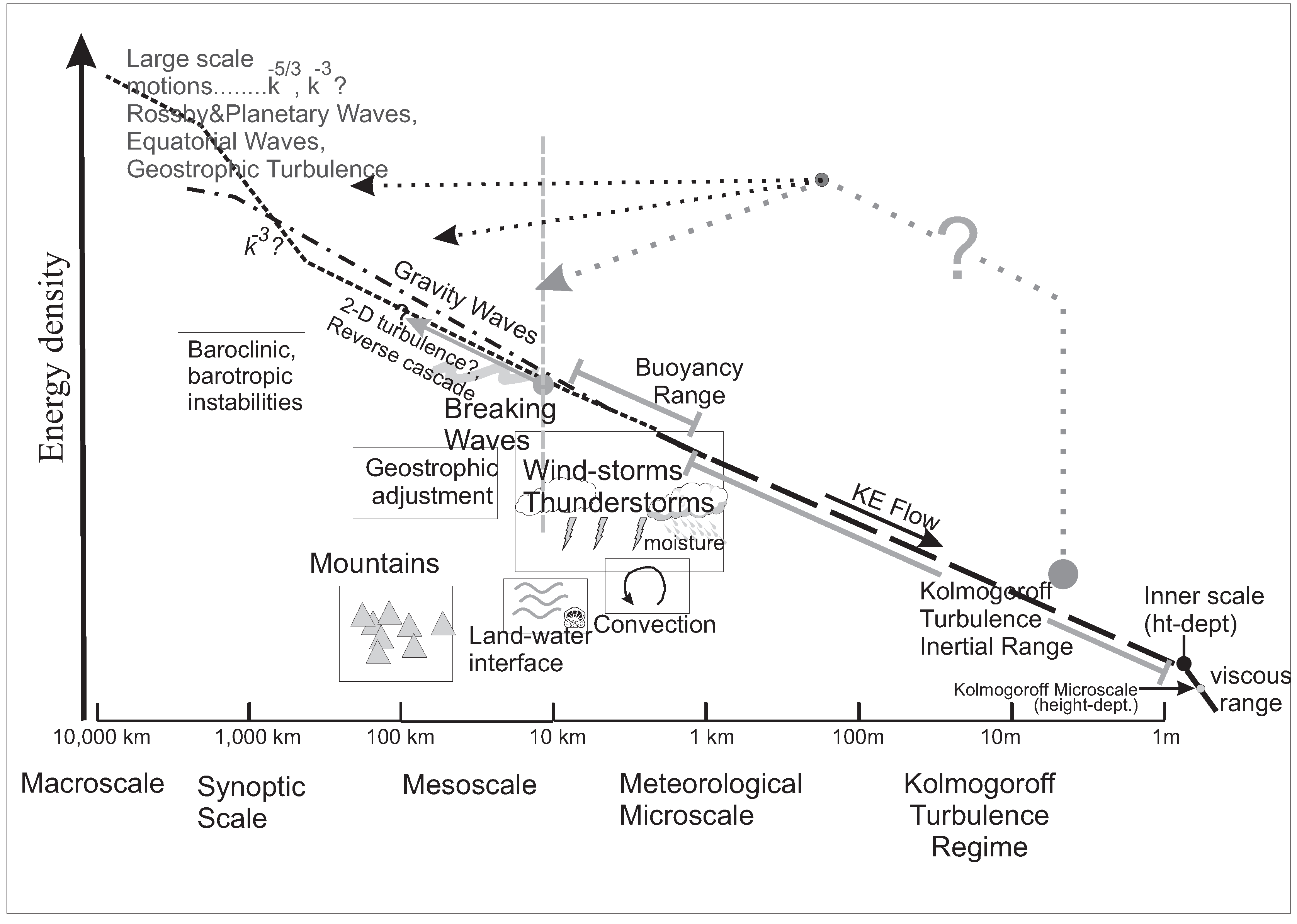
Figure 2.
Schematic illustration of particulate, potential temperature and/or momentum diffusion in regions of highly spatially intermittent turbulence. Fig (a) shows an isolated patch of turbulence, while Figure (b) shows the same region after the original layer has dissipated, but with a new layer formed slightly above the first. In (b), the “constituent density" of the original layer is close to constant, since it had been mixed to be that way while turbulence had existed there. Although we speak of “constituents”, the same applies to potential temperature, which also tends to constant values as a function of height during mixing. See text for more details.
Figure 2.
Schematic illustration of particulate, potential temperature and/or momentum diffusion in regions of highly spatially intermittent turbulence. Fig (a) shows an isolated patch of turbulence, while Figure (b) shows the same region after the original layer has dissipated, but with a new layer formed slightly above the first. In (b), the “constituent density" of the original layer is close to constant, since it had been mixed to be that way while turbulence had existed there. Although we speak of “constituents”, the same applies to potential temperature, which also tends to constant values as a function of height during mixing. See text for more details.
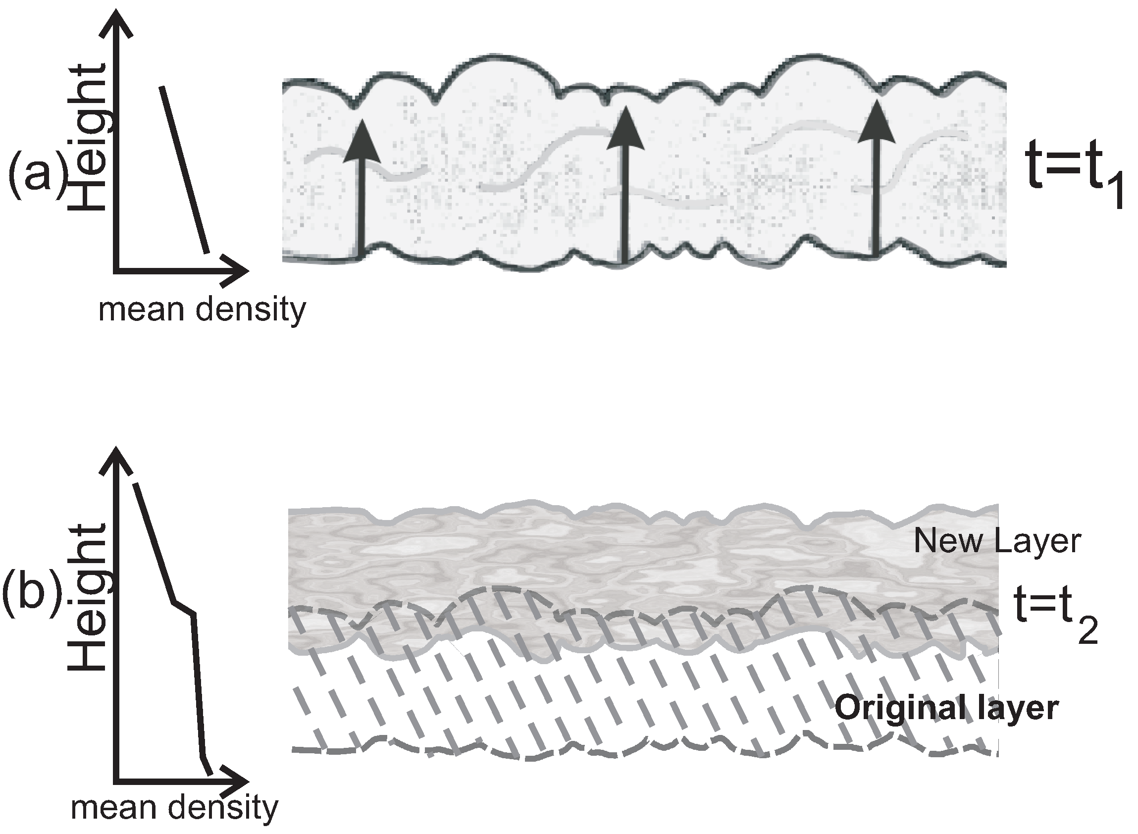
Figure 3.
(a) Total “orbit” of a set of harmonically related waves with periods of 240 mins., 120 mins., … 6.25 mins. over a time of 240 mins. (b) Conceptual diagram of the Stokes drift for a gravity wave in a compressible atmosphere and (c) action of a turbulent patch in enhancing diffusion by transferring particles between isentropic surfaces. See text for details.
Figure 3.
(a) Total “orbit” of a set of harmonically related waves with periods of 240 mins., 120 mins., … 6.25 mins. over a time of 240 mins. (b) Conceptual diagram of the Stokes drift for a gravity wave in a compressible atmosphere and (c) action of a turbulent patch in enhancing diffusion by transferring particles between isentropic surfaces. See text for details.
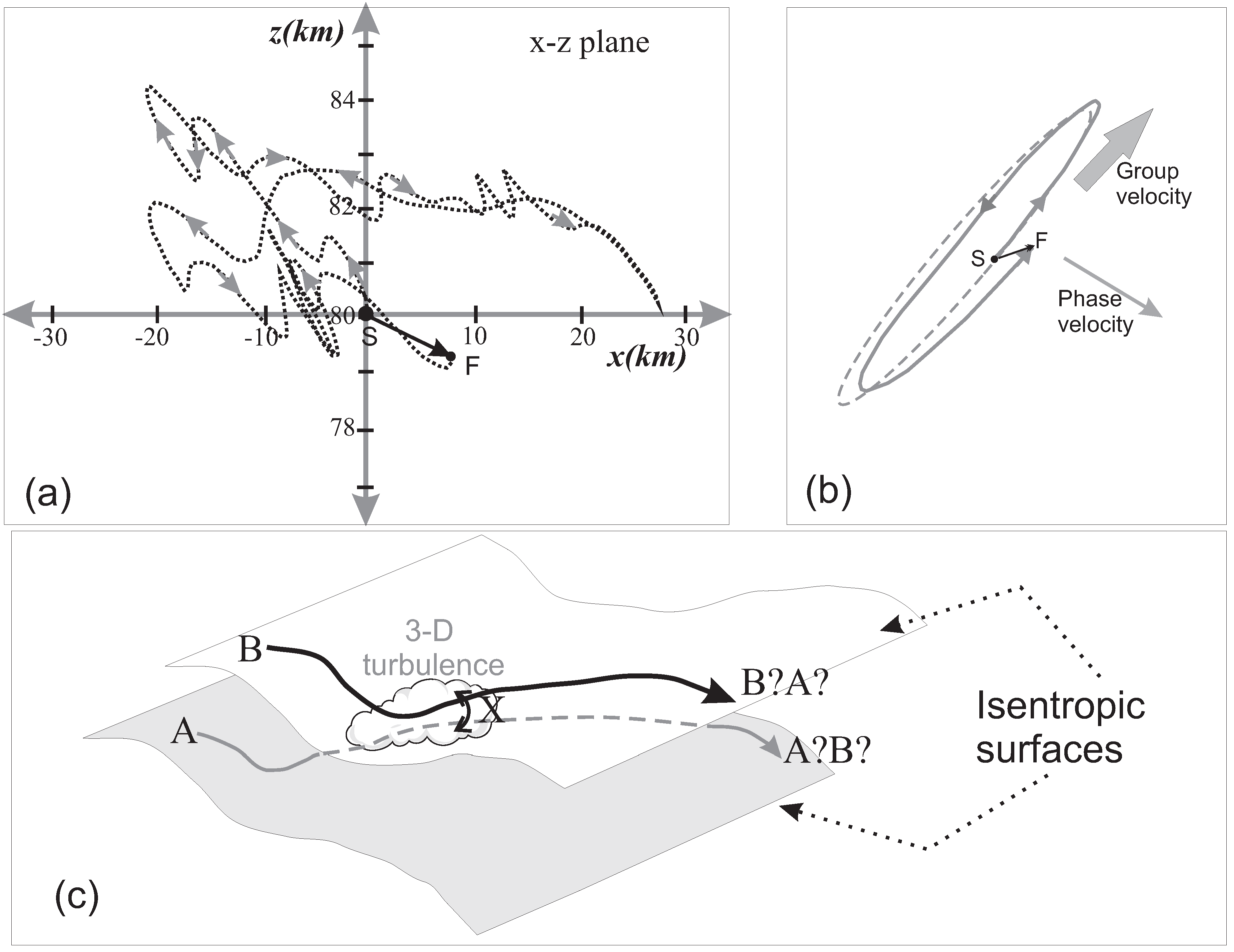
Figure 4.
Figure 1 from [89], with corrections. The original paper missed the gravity wave branch which is clearly evident with a power law between 200 and 900 km. See text for details.
Figure 4.
Figure 1 from [89], with corrections. The original paper missed the gravity wave branch which is clearly evident with a power law between 200 and 900 km. See text for details.
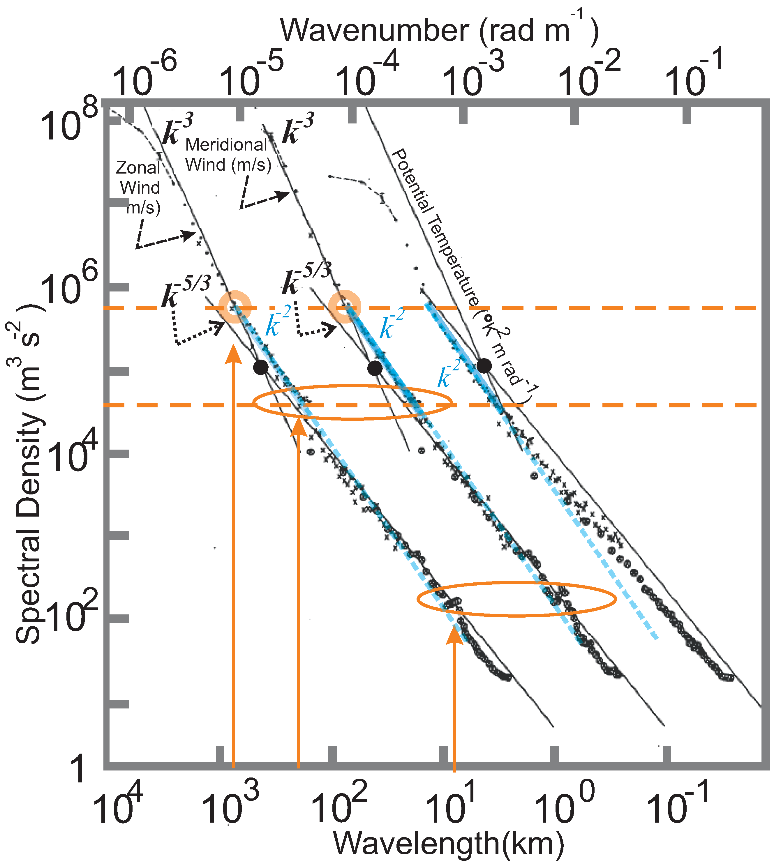
Figure 5.
Expanded view of Figure 4 concentrating around the region of the gravity-wave power law. A best-fit straight line (based on standard gravity-wave theory e.g. [31]) is shown in blue.
Figure 5.
Expanded view of Figure 4 concentrating around the region of the gravity-wave power law. A best-fit straight line (based on standard gravity-wave theory e.g. [31]) is shown in blue.
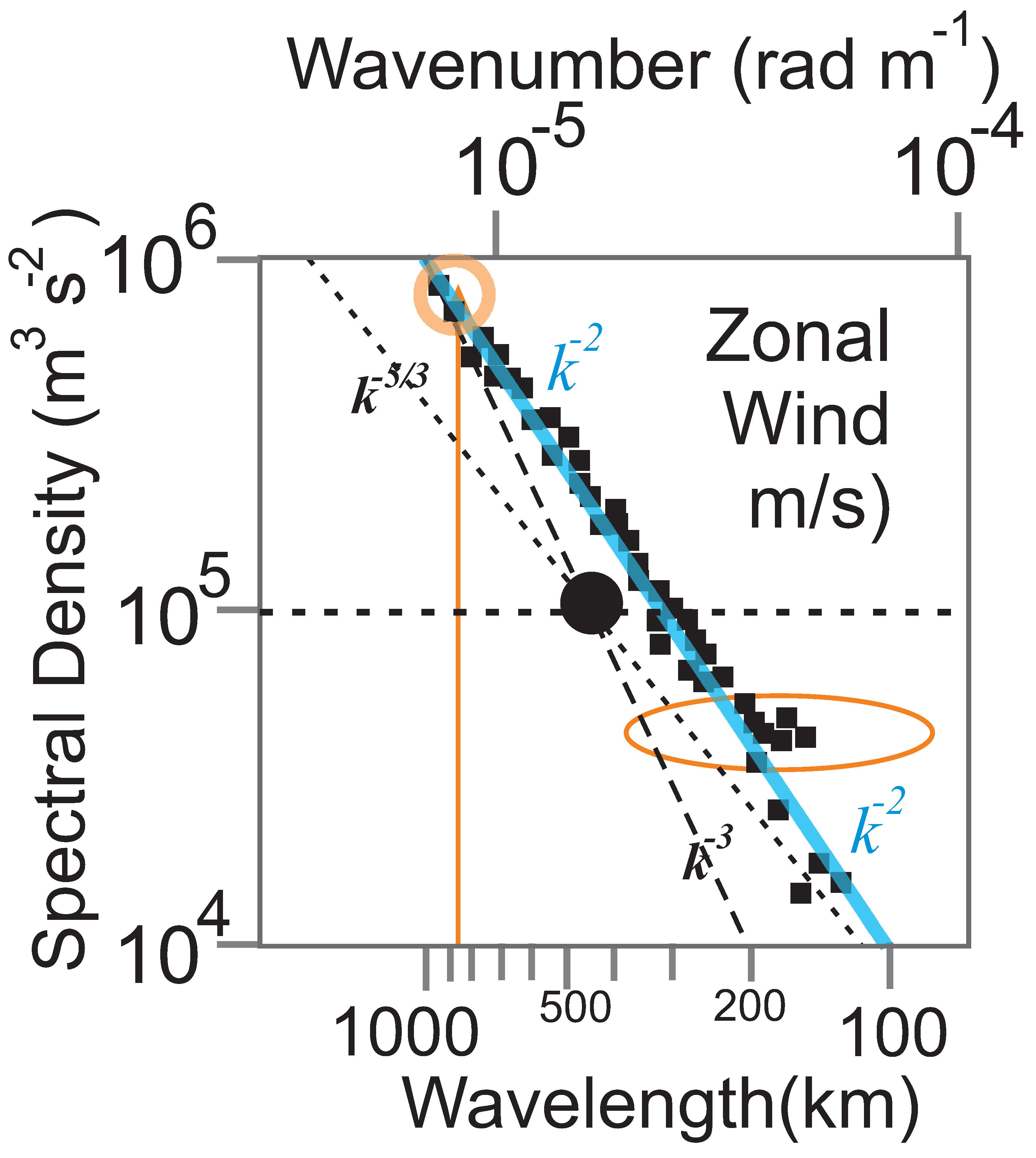
Figure 6.
Contour plot of the vertical diffusion coefficients used in [90] for January (provided from the WACCM6 model [90] by Dr. Rolando Garcia of the U.S. National Center for Atmospheric Research (NCAR), Atmospheric Chemistry Observations and Modeling Laboratory). See text for details.
Figure 6.
Contour plot of the vertical diffusion coefficients used in [90] for January (provided from the WACCM6 model [90] by Dr. Rolando Garcia of the U.S. National Center for Atmospheric Research (NCAR), Atmospheric Chemistry Observations and Modeling Laboratory). See text for details.
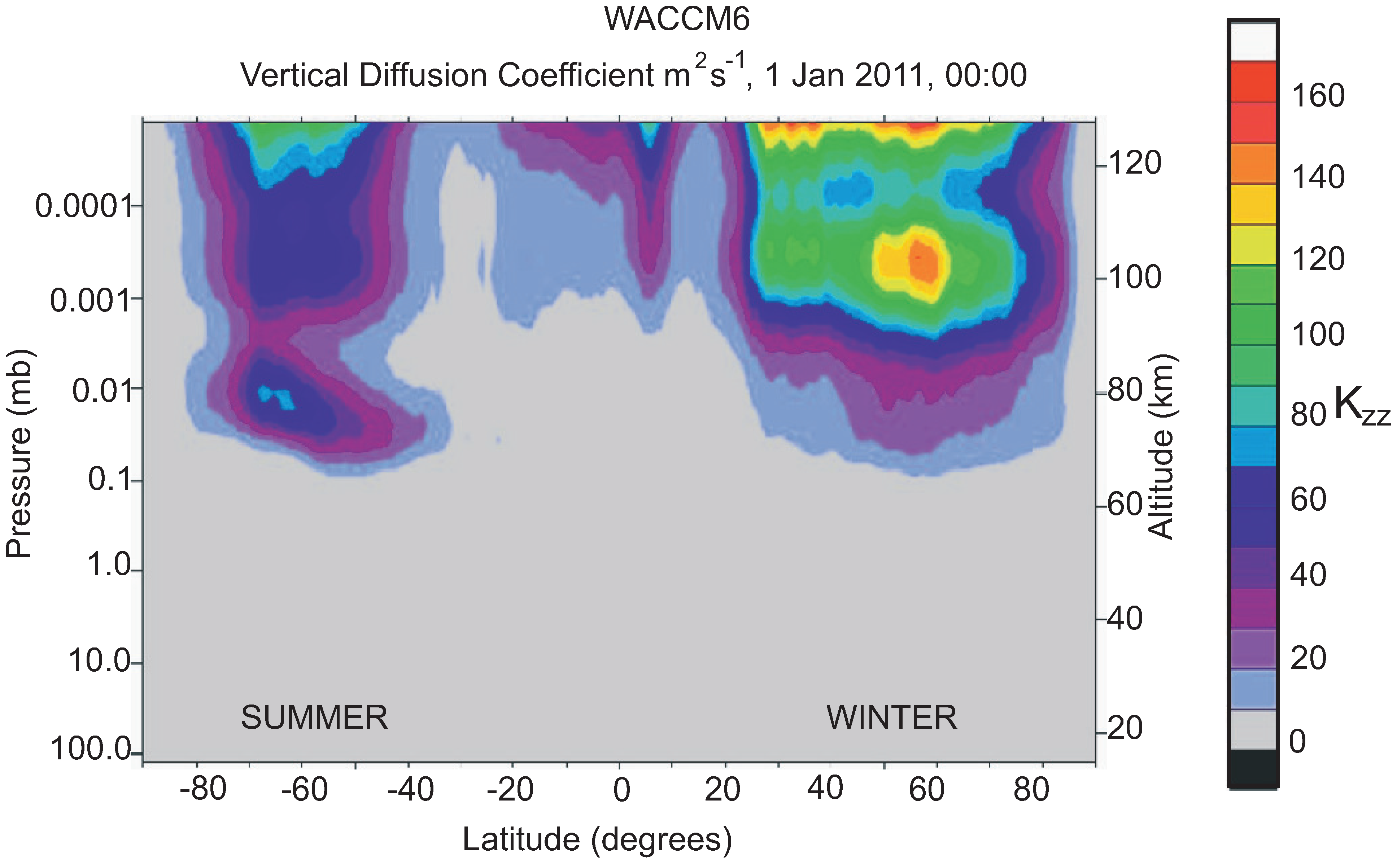
Figure 7.
Effective ”diffusion coefficients” for a JAGUAR run using 96 hours of data from June 1-4, 2022. See text for details.
Figure 7.
Effective ”diffusion coefficients” for a JAGUAR run using 96 hours of data from June 1-4, 2022. See text for details.
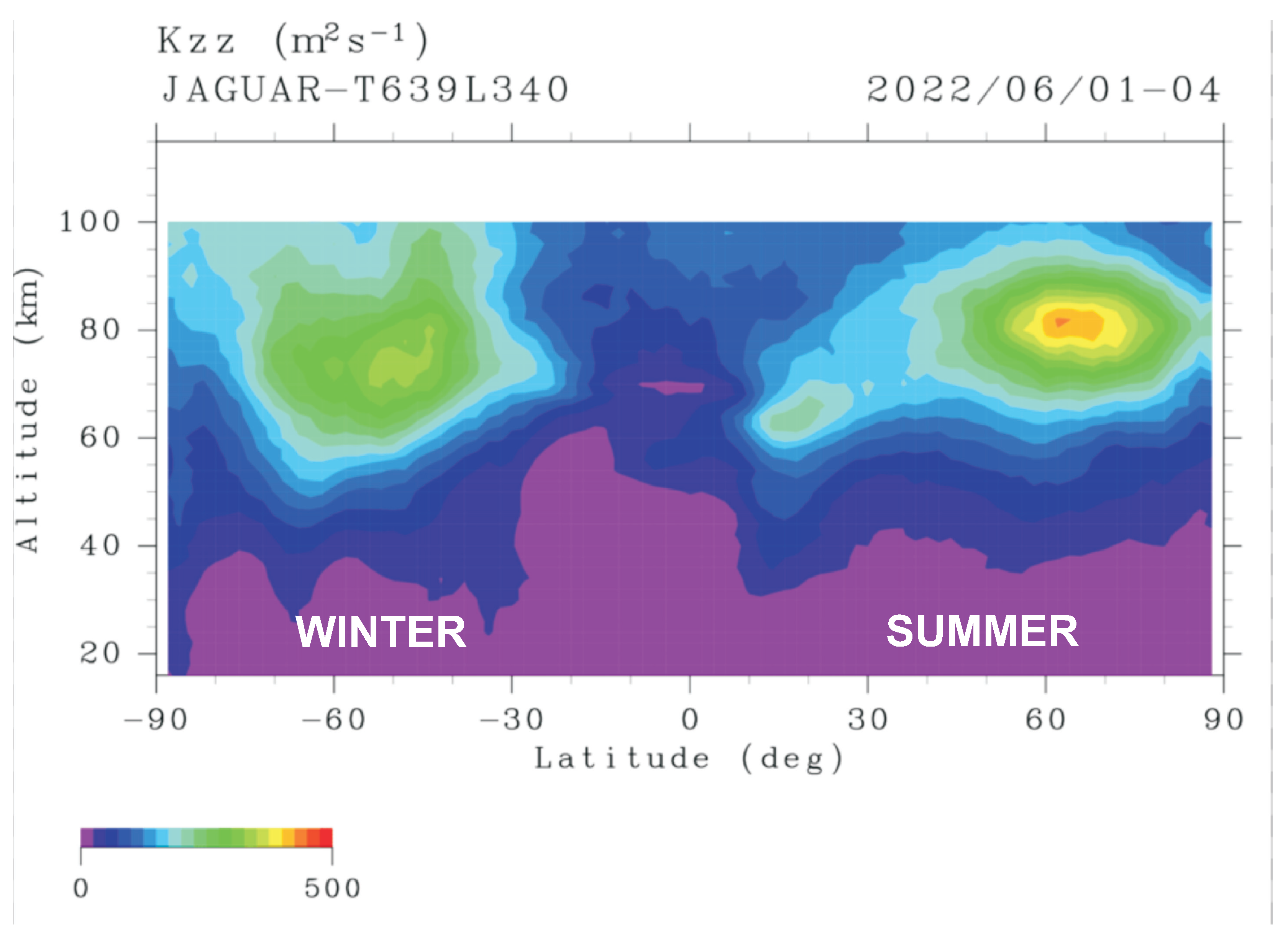
Disclaimer/Publisher’s Note: The statements, opinions and data contained in all publications are solely those of the individual author(s) and contributor(s) and not of MDPI and/or the editor(s). MDPI and/or the editor(s) disclaim responsibility for any injury to people or property resulting from any ideas, methods, instructions or products referred to in the content. |
© 2026 by the authors. Licensee MDPI, Basel, Switzerland. This article is an open access article distributed under the terms and conditions of the Creative Commons Attribution (CC BY) license (http://creativecommons.org/licenses/by/4.0/).
Copyright: This open access article is published under a Creative Commons CC BY 4.0 license, which permit the free download, distribution, and reuse, provided that the author and preprint are cited in any reuse.