
Submitted:
09 August 2026
Posted:
11 August 2026
You are already at the latest version
Abstract
Short-term fluctuations in reference signal received power (RSRP) under high-mobility conditions can repeatedly reset the time-to-trigger (TTT) timer and cause spatial dispersion of Event A3 handover triggers in high-speed railway 5G-R systems. To address this problem, this study develops a physics-driven, Doppler-aware RSRP input-calibration framework that preserves the standardized handover margin (HOM), TTT, Event A3 semantics, and Radio Resource Control (RRC) procedure. The relative residual Doppler shift is derived from train kinematics and base-station geometry and estimated online using a scalar Kalman filter. The resulting estimate is mapped to an orthogonal frequency-division multiplexing frequency-offset-induced equivalent RSRP loss subject to a physical upper bound. Geometry-based detrending, speed-adaptive causal smoothing of the residual component, and a low-weight bounded position-aided correction are subsequently applied to reconstruct the serving- and candidate-cell RSRP inputs. Event-driven simulations covering viaduct and mountainous railway scenarios, together with ablation, Doppler-sensitivity, speed-adaptability, and observation-error analyses, are conducted to evaluate the proposed method. At a train speed of 350 km/h, the method reduces the root-mean-square error of the inter-cell RSRP difference from 2.3449 to 1.9053 dB and decreases the mean handover trigger-location error from 54.79 to 42.35 m, while maintaining a handover success rate of 99.49%, comparable to the 99.29% achieved by conventional Event A3. The results further demonstrate that, under a carrier frequency of 2.1 GHz and a subcarrier spacing of 30 kHz, the overall performance improvement is governed primarily by geometric detrending, speed-adaptive residual smoothing, and bounded position correction, whereas Doppler-loss compensation provides a small but physically consistent correction of the deterministic measurement bias. The proposed framework therefore improves RSRP input quality and handover trigger-location consistency without modifying the standardized handover decision logic.
Keywords:
5G-R
; high-speed railway communications
; Doppler-aware handover
; RSRP measurement calibration
; Event A3
; mobility management
1. Introduction
With the continuous expansion of urbanization and transportation infrastructure, the construction of underground transportation facilities and linear railway systems has been rapidly increasing worldwide, resulting in more complex engineering and operational environments [1,2,3]. And the rapid digitalization and intelligent transformation of railway systems are placing increasingly stringent demands on train-ground wireless communications. In addition to conventional voice and dispatching services, next-generation railway communication networks are expected to support automatic train operation, real-time condition monitoring, high-definition video transmission, intelligent maintenance, and other safety-critical or bandwidth-intensive applications. Fifth-generation communication for railways (5G-R) has therefore emerged as a promising successor to the narrowband Global System for Mobile Communications-Railway (GSM-R), owing to its enhanced capacity, low latency, massive connectivity, and flexible service architecture [4,5]. Nevertheless, railway cellular networks differ fundamentally from conventional terrestrial networks because they are deployed along elongated linear corridors and serve groups of users moving synchronously at very high speeds. The resulting non-stationary propagation, shortened cell residence time, rapid signal variation, and frequent handovers present substantial challenges to service continuity and mobility management.
A fundamental prerequisite for addressing these challenges is an accurate understanding of the time-varying railway propagation channel. Zhou et al. [5] conducted delay-Doppler-domain measurements at a train speed of 371 km/h and established channel models for different time-varying conditions, revealing that the quasi-invariant intervals of channel fading coefficients occur on a millisecond scale. To characterize channel non-stationarity more comprehensively, Zhang et al. [6] introduced a joint Doppler-delay power-profile method and identified distinct quasi-stationary-region characteristics in viaduct and cutting environments. Measurement-based studies have also demonstrated substantial scenario dependence in railway propagation. Zhang et al. [7] investigated delay dispersion and Doppler characteristics in mountainous railway terrain and developed a tapped-delay-line model incorporating position-dependent multipath behaviour. More recently, Chen et al. [8] used passive measurements to quantify the additional large-scale losses introduced by buildings, viaducts, and depot-like structures in a 2100 MHz 5G-R network. At higher carrier frequencies, Gong et al. [9] investigated Doppler compensation for high-speed railway communications over mmWave bands and developed data-aided strategies to mitigate Doppler-induced performance degradation. These studies demonstrate that Doppler behaviour, multipath evolution, and received-power variation are strongly coupled with carrier frequency, train position, and the surrounding railway environment.
Building on these channel-characterization studies, considerable attention has been devoted to Doppler-frequency estimation and compensation. Tang et al. [10] developed cross-ambiguity-function-based Doppler estimators with performance approaching the Cramér-Rao lower bound, while maintaining lower computational complexity than least-squares estimation. Hou et al. [11] incorporated prior Doppler information from a radio environment map into a maximum a posteriori estimator for LTE-R systems, thereby improving both estimation accuracy and bit-error-rate performance. For line-of-sight-dominated high-speed railway channels, Yang et al. [12] separated the dominant line-of-sight component from multipath propagation to improve Doppler-frequency-offset estimation. In the millimeter-wave domain, Zhang et al. [13] proposed three Doppler-shift estimators and demonstrated that an enhanced equally divided structure-based estimator could approach its theoretical performance bound. Data-driven methods have also been explored: Kim et al. [14] developed an RSRP-based machine-learning Doppler estimator with an ambiguity-reduction mechanism, whereas Li et al. [15] exploited the joint relationship between azimuth and Doppler frequency to improve the speed estimation of nearby tangential targets. Collectively, these methods provide effective means of recovering Doppler or motion information, although their performance is generally assessed in terms of frequency-estimation error, bit-error rate, or target-speed accuracy rather than the stability of cellular handover measurements.
The physical relationship between Doppler information and terminal motion has further motivated its application in localization, navigation, and integrated sensing. He et al. [16] incorporated Doppler mitigation into an adaptive UWB/IMU fusion framework to improve high-speed-train localization. In satellite navigation, Gao and Xia [17] combined Doppler-frequency estimation, frequency compensation, and data-bit transition processing to accelerate weak GNSS signal acquisition. Cao and Chen [18] reconstructed acoustic reference signals according to the estimated relative speed between a mobile terminal and a base station, thereby reducing Doppler-induced positioning errors. For 5G-based railway positioning, Wen et al. [19] developed a higher-order improved extended Kalman filter that uses nonlinear statistical information to enhance localization accuracy. Li et al. [20] further employed delay-Doppler channel estimates in an orthogonal time-frequency space-based integrated sensing and communication framework, jointly estimating target motion and transmitter location through weighted least squares and semidefinite relaxation. These studies confirm that Doppler observations can provide valuable physical priors for motion-state estimation; however, their primary objectives are localization or environmental sensing rather than the calibration of measurements used by standardized cellular handover procedures.
At the mobility-management level, reliable reference signal received power (RSRP) measurement and appropriate handover triggering are essential for maintaining train-ground connectivity. Park and Park [21] derived closed-form expressions for the mean and mean-squared errors of LTE RSRP measurements and demonstrated the dependence of the optimum averaging configuration on the signal-to-interference-plus-noise ratio and channel delay spread. Based on RSRP variation, Cho et al. [22] proposed a handover-point control scheme that reduced handover failures at train speeds of up to 500 km/h. Wu et al. [23] developed a temporal-difference-learning framework to adapt LTE-R handover parameters to changing train speeds and network conditions. Instead of relying solely on received-signal measurements, Aguado et al. [24] proposed a cross-layer mobility-pattern-aware strategy incorporating train position, speed, network conditions, and traffic profiles to schedule IEEE 802.16 handovers. Polaganga and Liang [25] subsequently used ensemble learning and live 5G NR standalone network data to predict RRC Resume and Fallback transitions, enabling proactive context management while preserving signaling latency. These studies have substantially advanced handover control, parameter adaptation, and state prediction, but the measured RSRP is commonly treated as an externally supplied input rather than a physical quantity requiring systematic calibration before the handover decision.
To address the instability of A3 handover triggering caused by short-term RSRP fluctuations in high-speed railway 5G-R communications, this study proposes a physics-driven, low-complexity RSRP input calibration method that remains fully compatible with the standard A3 procedure. The method integrates Kalman-filter-based residual Doppler estimation, physically bounded Doppler-loss compensation, geometric-trend removal, speed-adaptive causal smoothing, and bounded position-based correction to reconstruct the serving- and candidate-cell RSRP inputs. Its effectiveness and robustness are evaluated through ablation, speed, Doppler-sensitivity, and multi-scenario simulations covering viaduct and mountainous railway environments.
2. System Model and Problem Description
To investigate the impact of RSRP measurement bias on A3 event triggering under high-mobility conditions, a two-cell linear coverage scenario for high-speed railway communications is established. Under a unified geometric framework, the link distance, Doppler shift, and RSRP observation process are characterized. Based on this framework, a mapping relationship between the relative residual Doppler shift and the equivalent RSRP loss is derived, thereby defining the optimization objective and constraints for input calibration.
2.1. The Switching Between Two High-Speed Railway Cells and the A3 Mechanism
High-speed railway communication systems typically employ continuous strip-shaped cellular coverage along the railway line, where trains undergo rapid serving-cell transitions within the overlapping regions of adjacent cells. Because the A3 event is triggered based on the measurement difference between a candidate cell and the serving cell, together with the duration for which the triggering condition is satisfied, both systematic RSRP bias and short-term fluctuations may alter the handover trigger location.
Consider a serving base station S and a candidate base station T deployed in a chain topology along the railway, with their projected coordinates on the track axis given by 0 and D, respectively. The lateral distance from each base station to the track is , and the height difference between the base-station antenna and the onboard antenna is −. The train travels in the positive direction at a speed of v, and its position is denoted by x. Accordingly, the geometric distances of the serving and candidate links are expressed as:
Where and are the three-dimensional distances from the train at longitudinal coordinate to the serving and target base stations, respectively, is the along-track separation between the two base-station projections, is the perpendicular distance from each base station to the track, and and are the base-station and onboard-antenna heights.
Figure 1.
The Geometric Topology of the Switching between Two Cells of the 5G-R High-speed Railway.
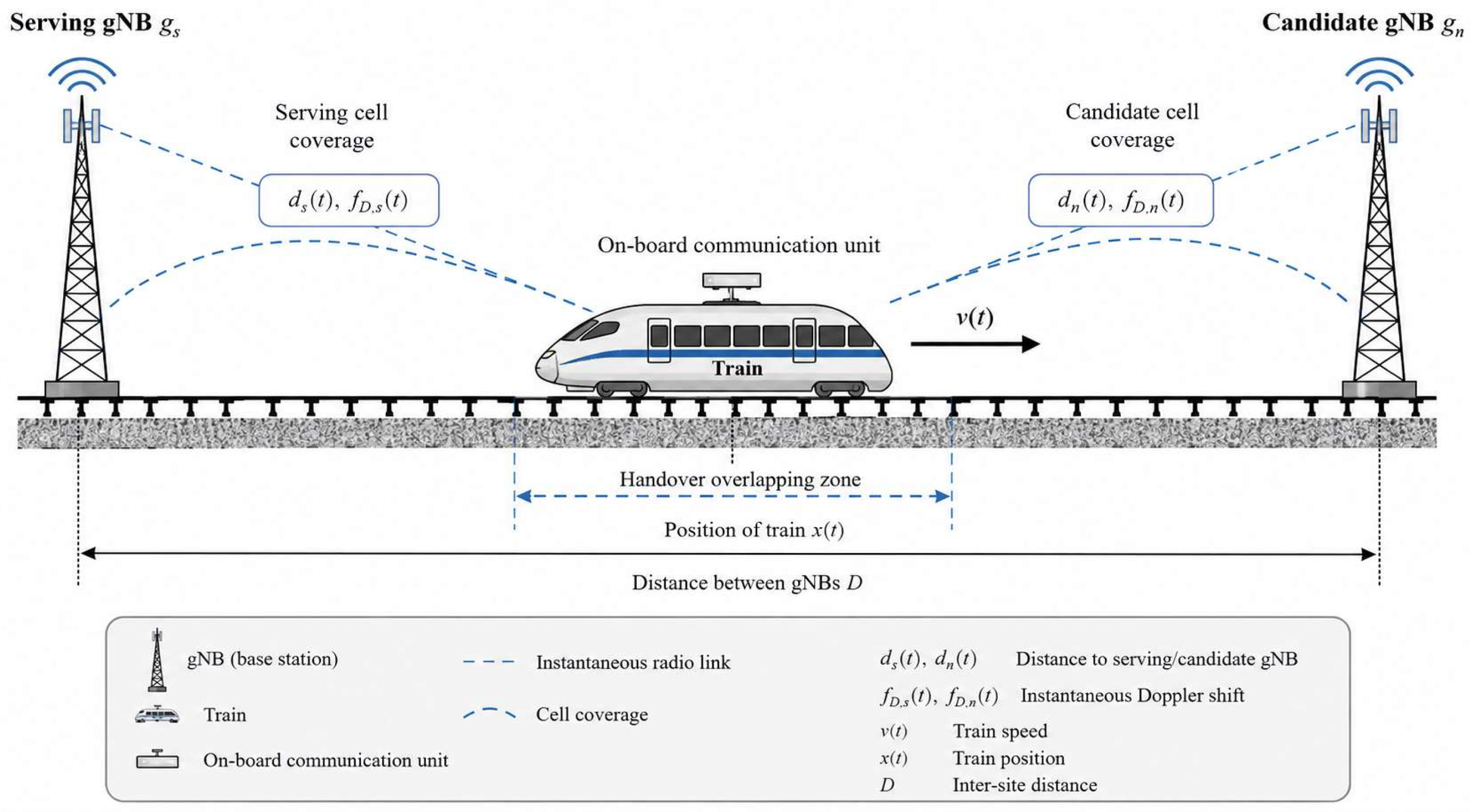
The model assumes that the train travels at an approximately constant speed within a single handover region. The base-station coordinates and antenna parameters are assumed to be known, while the train position and velocity can be obtained from the Global Navigation Satellite System GNSS or the railway traffic management system. The serving and candidate cells operate with the same carrier frequency and subcarrier configuration. The propagation model accounts for large-scale path loss, spatially correlated shadow fading, and measurement noise, whereas small-scale fast fading is partially averaged out through physical-layer measurement filtering.
Let Pt(k) and Ps(k) denote the A3 input measurements of the candidate cell and the serving cell, respectively, at the k-th measurement instant. The corresponding cell-specific offsets are denoted by Ot and Os, and the handover hysteresis margin is denoted by HOM. The Event A3 entry condition and the number of consecutive samples required to satisfy the time-to-trigger (TTT) criterion are expressed as:
Where is the minimum number of consecutive measurement samples required to satisfy Event A3, is the time-to-trigger duration, is the RSRP measurement interval, and denotes the ceiling operation.
A measurement report for handover is triggered only when the condition in Eq. (2) remains satisfied for consecutive measurement periods. If the candidate-cell measurement is persistently underestimated, the trigger location shifts toward the rear portion of the cell-overlap region. Conversely, if random fluctuations cause the condition to be satisfied continuously at an earlier position, a premature handover may occur. Let denote the ideal trigger location, the actual trigger location, and the local slope of the coverage-power difference. Under the small-bias approximation, the following relationship holds:
Where is the approximate trigger-location displacement caused by an inter-cell RSRP error , and is the local spatial gradient of evaluated at .
Eq. (4) indicates that the handover-location error is not determined solely by the HOM and TTT parameters. Measurement-input bias is also mapped into a spatial displacement through the local slope of the coverage-power difference. Therefore, while preserving the standard Event A3 and TTT logic, calibrating the RSRP inputs prior to the handover decision provides a feasible approach for improving the consistency of handover trigger locations. To identify the error components that require calibration, a Doppler and RSRP observation model under high-mobility conditions is further established.
2.2. Doppler and RSRP Measurement Models
During high-speed train operation, the serving and candidate links exhibit different radial-velocity projections, resulting in a relative Doppler difference between the two links. This difference may cause a deterministic loss of useful OFDM signal energy, whereas shadow fading and measurement noise introduce random fluctuations into the RSRP observations. To distinguish among these error sources, a model incorporating the signed Doppler shift, relative residual Doppler shift, geometric coverage trend, and composite RSRP observation is established. Based on the radial-velocity projections, the signed Doppler shifts of the serving and candidate links are respectively expressed as:
Where and are the signed Doppler shifts of the serving and target links at position , is the carrier frequency, is the train velocity, is the speed of light, and the signs follow the adopted radial-motion convention.
When the receiver uses the serving cell as its primary synchronization reference, the relative residual Doppler shift affecting the candidate-cell measurement and the corresponding frequency offset normalized by the subcarrier spacing are defined as:
Where is the relative residual Doppler offset between the target and serving links, is the OFDM subcarrier spacing, and is the corresponding normalized frequency offset.
denotes the effective frequency offset of the candidate cell relative to the serving-cell measurement reference; it is not equivalent to the absolute residual frequency offset remaining after physical-layer frequency tracking. The geometric coverage trend of cell i, excluding random perturbations, is represented using the log-distance path-loss model as:
Where is the geometry-dependent RSRP trend of cell , is the received power at reference distance , is the path-loss exponent, is the link distance, and is the additional loss associated with the propagation environment.
For an OFDM system with an N-point FFT, the normalized frequency offset reduces the useful-signal energy coefficient of the target subcarrier to:
where is the useful subcarrier-energy coefficient under normalized frequency offset , is the FFT size, and =/ denotes the normalized function used in the large- approximation.
Where is the Doppler-induced equivalent RSRP loss in decibels, is the useful-energy coefficient defined in Eq. (8), and is the second-order small-offset approximation of .
Under the small-frequency-offset approximation, Eq. (9) establishes the approximate relationship between the normalized frequency offset and the equivalent RSRP loss. For a carrier frequency of 2.1 GHz, a train speed of 350 km/h, and a subcarrier spacing of 30 kHz, the maximum relative Doppler shift is approximately 1.36 kHz, yielding ε is 0.045 and a corresponding loss of approximately 0.03 dB. This value is substantially smaller than the shadow-fading variation of approximately 3-5 dB. Accordingly, the candidate-cell measurement model can be expressed in a unified form as:
Where is the measured target-cell RSRP, is its geometry-dependent component at train position , is the deterministic frequency-offset loss, and , , and represent shadow fading, measurement noise, and anomalous observation bias, respectively.
As indicated by Eq. (10), the components to be addressed include the deterministic frequency-offset-induced loss and the observation perturbations that can be suppressed through filtering, whereas shadow fading caused by actual physical blockage should be retained as part of the channel state. This decomposition provides a physical basis for the subsequent component-specific calibration.
2.3. Research Objectives and Constraints
Based on the preceding error decomposition, the calibration objectives are defined as reducing the RMSE of the candidate-cell RSRP and the inter-cell RSRP difference, minimizing the handover trigger-location error, and controlling the radio link failure RLF rate and ping-pong handover rate without degrading the handover success rate. To balance real-time operation, physical interpretability, and protocol compatibility, the proposed method uses only current and historical observations, maintains an O(1) online computational complexity per sample, and constrains the compensation magnitude by an explicit physical upper bound. When positioning information is unavailable, the method degrades gracefully to Doppler compensation combined with causal smoothing. The entire calibration procedure preserves the standard Event A3 semantics, HOM, TTT, and the RRC handover process.
These objectives and constraints jointly define the algorithmic design boundary: handover trigger-location consistency is improved by enhancing the quality of the measurement inputs, rather than by modifying the decision thresholds or excessively compensating for genuine channel attenuation to obtain apparent performance gains.
3. Doppler Sensing RSRP Input Calibration Method
According to the preceding observation model, the RSRP bias can be decomposed into deterministic Doppler-induced equivalent loss, the position-dependent geometric coverage trend, random observation perturbations, and genuine shadow fading. Based on the distinct physical characteristics of these components, a four-stage input-calibration framework is developed, comprising relative residual Doppler estimation, physically bounded compensation, geometric detrending combined with speed-adaptive residual smoothing, and position-based differential correction.
3.1. Overall Framework
Figure 2 illustrates the overall workflow of the RSRP input-calibration framework. The inputs include the serving- and candidate-cell RSRP measurements, train position and velocity, base-station geometric parameters, and system parameters such as the carrier frequency and subcarrier spacing. The outputs are the calibrated RSRP values of the two cells and their difference. The processing chain sequentially comprises state acquisition, relative residual Doppler estimation, physical-loss compensation, geometric-trend removal, residual smoothing, position-based differential correction, and the standard Event A3 decision. The calibration module is inserted between measurement-report generation and the Event A3 decision, making it transparent to the upper-layer event semantics and the RRC signaling procedure.
3.2. Relative Residual Doppler Estimation
The relative residual Doppler shift varies continuously with the train position, whereas positioning, velocity-estimation, and frequency-observation errors primarily manifest as short-term random perturbations. To suppress observation noise while preserving the underlying spatial variation trend, the relative residual Doppler shift is modeled as a one-dimensional random-walk state and estimated online using a scalar Kalman filter. Let denote the relative residual Doppler state at the k-th instant, and let denote the observation calculated from the train position, velocity, and base-station topology. The state-space model is then expressed as:
Where, within the Doppler state-space model, and are the process and observation noise terms, respectively.
Where is the observation-noise variance at sample , , , and are the standard deviations of the position, velocity, and frequency-estimation errors, and the partial derivatives quantify the sensitivity of to position and velocity uncertainties.
The prediction, Kalman-gain calculation, and update recursions of the one-dimensional Kalman filter are given by:
Where and are the prior Doppler-state estimate and its error variance, and are the preceding posterior quantities, is the process-noise variance, is the observation-noise variance, and is the scalar Kalman gain.
Where and are the posterior state estimate and posterior error variance, is the measurement innovation, and is the estimated normalized frequency offset.
Because the filter contains only a single state variable, each recursion requires only scalar operations. It can therefore suppress zero-mean perturbations in positioning, velocity estimation, and frequency observations with low computational overhead, while tracking the dominant Doppler trend that varies continuously with the train position. The resulting estimate is subsequently used to determine the equivalent RSRP loss.
3.3. Doppler Equivalent Loss Compensation Under Physical Boundary Constraints
The equivalent RSRP loss calculated from the estimated frequency offset has a well-defined physical upper bound determined by the OFDM system. Direct compensation based on an anomalous frequency-offset observation may amplify the observation error into an unrealistic power correction. Therefore, the compensation upper bound is determined according to the maximum design speed, the base-station geometry, and the system subcarrier configuration. The equivalent loss of the candidate cell is calculated from ε̂k and defined as:
Where is the equivalent RSRP loss inferred from , is the physically admissible loss bound, and is the maximum relative residual Doppler offset permitted by the design velocity and cell geometry.
Where is the first-stage target-cell RSRP after Doppler-loss calibration, and limits the applied correction to the smaller of the estimated loss and its physical upper bound.
This compensation introduces no empirical gain; it only corrects the deterministic bias in the RSRP measurement caused by the frequency offset and should not be interpreted as recovering signal energy already lost at the physical layer. Under the current system parameters, is approximately 0.03 dB. Therefore, even when anomalous frequency-offset observations occur, the clipping mechanism prevents the compensation magnitude from exceeding the physically feasible range.
3.4. Geometric Trend Removal and Causal Residual Smoothing
After compensating for the deterministic frequency-offset-induced loss, the RSRP sequence still contains both the dominant coverage trend caused by distance variation and random observation residuals. Direct low-pass smoothing of the absolute RSRP would also delay the coverage trend, potentially shifting the Event A3 trigger location. Therefore, the geometric coverage trend is first removed according to Eq. (7), after which only the residual component is subjected to speed-adaptive causal smoothing before the corresponding trend is restored. The residual is defined as:
Where is the detrended RSRP residual of cell , is the first-stage calibrated RSRP, and is the geometry-dependent RSRP evaluated at the train position associated with sample .
The smoothing memory length is governed by the shadow-fading correlation distance . The weight assigned to the current sample and the corresponding causal recursion are given by:
Where is the velocity-adaptive weight assigned to the current residual sample, is the train velocity at measurement instant , is the sampling interval, and is the spatial correlation distance of shadow fading.
Where is the causally smoothed residual of cell , is its previous value, is the current detrended residual, and controls the balance between temporal smoothing and instantaneous tracking.
Where is the second-stage RSRP estimate of cell , obtained by restoring the geometry-dependent trend to the smoothed residual .
As the train speed increases, increases, causing the recursive filter to assign greater weight to the current sample and thereby reduce tracking lag. At lower speeds, decreases, which enhances the suppression of random noise. The geometric detrending-residual smoothing-trend restoration procedure preserves the overall slope of the inter-cell coverage difference within the overlap region while reducing repeated threshold crossings near the HOM.
3.5. Position-Constrained Correction and A3 Input Reconstruction
After frequency-offset compensation and residual smoothing, random perturbations in the inter-cell RSRP difference are substantially suppressed; however, a small number of anomalous observations may still shift the handover trigger location. Given the strong spatial determinism of high-speed railway tracks and base-station topology, a low-weight, bounded position prior is introduced to assist in correcting the inter-cell RSRP difference. This position constraint neither replaces the actual measurements nor compensates for genuine shadow fading. The second-stage processed difference, the geometric difference, and the bias to be corrected are defined as:
Where is the target-to-serving RSRP difference after residual smoothing, is the corresponding geometry-derived difference, and measures the deviation of the processed RSRP difference from the geometric reference.
Where is the final calibrated inter-cell RSRP difference, is the position-correction weight, is the correction bound, and constrains to the interval .
When positioning information is unavailable, β is set to zero, and the calibration output naturally reduces to the result of Doppler compensation and causal smoothing. When valid positioning information is available, the position prior applies only a limited correction to inter-cell RSRP differences that deviate substantially from the geometric coverage relationship. The final calibrated measurements, and , are then directly fed into the standard Event A3 criterion and TTT timer.
3.6. Computational Complexity and Protocol Compatibility
All of the preceding processing stages are implemented using recursive or closed-form operations. Each measurement period involves only a scalar Kalman update, a first-order causal recursion, geometric-parameter calculations, and a small number of elementary operations. The resulting online computational complexity is O(1), with no iterative optimization required. Compared with Grey-Markov historical-window fitting and online neural-network inference, the proposed method imposes a lower computational burden. The calibration module can be deployed either in the RRC measurement-processing procedure at the base-station side or in the measurement-report generation procedure at the onboard terminal. When positioning fails, the position-based correction is disabled; if the module malfunctions, the system falls back to the original RSRP inputs. Neither mechanism requires modification of the existing standardized interfaces.
4. Simulation Setup
To evaluate the impact of input calibration on RSRP measurement accuracy and Event A3 triggering behavior, an event-driven simulation model with two adjacent cells is developed for a high-speed railway scenario. The simulation encompasses both viaduct and mountainous propagation environments. To ensure a fair comparison between the proposed method and representative handover strategies, all methods are evaluated using identical train trajectories, channel realizations, and handover execution delays.
4.1. Scenario, Channel, and Parameter Settings
An event-driven simulation of two adjacent cells is implemented in MATLAB. The viaduct scenario adopts a path-loss exponent of 2.20, a shadow-fading standard deviation of 4.1 dB, and an additional loss of 0 dB, whereas the mountainous scenario uses a path-loss exponent of 2.55, a shadow-fading standard deviation of 3.3 dB, and an additional loss of 4 dB. Figure 3 illustrates the theoretical path-loss differences between the two scenarios. The equivalent reference-signal transmit power is back-calculated by setting the RSRP at a cell-edge distance of 1300 m to -110 dBm, thereby avoiding the direct use of the total base-station transmit power as the RSRP.
Spatially correlated shadow fading is generated using a first-order spatial autoregressive process:
Where is the spatially correlated shadow-fading sample, is the correlation coefficient between adjacent measurement locations, is the shadow-fading standard deviation, is the innovation term.
After establishing the deterministic path-loss and spatially correlated shadow-fading models, independent measurement noise and Doppler observation perturbations jointly induced by positioning, velocity-estimation, and frequency-observation errors are further superimposed to generate the complete simulated RSRP sequences. In addition to the fixed parameters listed in Table 1, all methods use identical train trajectories, channel samples, and random seeds. The number of repeated simulation runs is also provided in Table 1. Statistical results are reported as sample means together with the corresponding confidence intervals.
4.2. Compare the Algorithm with the Evaluation Index
To distinguish among the three technical pathways of measurement-input calibration, time-series prediction, and handover-parameter optimization, the conventional Event A3 method, the Grey-Markov prediction method, the IGWO-RBF parameter-optimization method, and an Event A3 method that directly applies causal smoothing to the raw RSRP measurements are selected as benchmarks. All methods use identical train trajectories, channel samples, handover execution delays, and random seeds. For the IGWO-RBF model requiring training, the test data are excluded from the training process. Ping-pong handover is uniformly defined as the reverse Event A3 condition being continuously satisfied again within 3 s after successful completion of the forward handover. Input accuracy is evaluated using the RMSEs of the candidate-cell RSRP and the inter-cell RSRP difference:
Where is the target-cell RSRP root-mean-square error, is the number of evaluated samples, and and are the calibrated and reference RSRP values for sample , respectively, with the summation taken over .
Where is the root-mean-square error of the inter-cell RSRP difference, and and are the calibrated and reference inter-cell differences for the -th sample, respectively.
Using the trigger location x*, obtained from the disturbance-free measurement sequence under the same HOM and TTT settings, as the reference, the handover trigger-location error and the composite performance metric are defined as:
Where is the absolute trigger-location error, is the trigger location obtained from the evaluated handover procedure, and is the reference trigger location derived from the disturbance-free RSRP sequence.
Where , , and denote the handover success rate, radio-link-failure rate, and ping-pong rate, respectively, , , and are their event counts, and is the total number of handover trials.
A handover is considered successful if the target-cell RSRP exceeds the access threshold upon completion of the handover execution and the serving-cell RSRP does not remain continuously below the RLF threshold before completion. The handover success rate is interpreted using the Wilson 95% confidence interval.
5. Simulation Results and Analysis
The proposed method is evaluated according to the logical sequence of state estimation, input calibration, triggering behavior, and scenario robustness. The independent contribution of each module is first identified through stagewise processing and ablation analysis. Performance variations under different Doppler levels and train speeds are then examined and compared with those of representative methods. Finally, the effects of propagation scenarios and observation-error variations on algorithmic stability are analyzed.
5.1. Calibration Mechanism and Ablation Analysis
The stagewise calibration results are used to verify whether each processing stage acts on its intended error component, while the ablation analysis further quantifies the independent contribution of each module to the accuracy of the inter-cell RSRP difference and the handover trigger location. In the representative simulation realization shown in Figure 4, the relative residual Doppler shift varies continuously with the train position, whereas the raw observations contain high-frequency perturbations of approximately 20-25 Hz. In this realization, the one-dimensional Kalman filter successfully tracks the dominant Doppler trend, reducing the estimation RMSE from approximately 25 Hz to approximately 8 Hz. Figure 5 further presents the stagewise processing results. Doppler compensation increases the candidate-cell RSRP by only approximately 0.03 dB overall; geometric detrending and residual smoothing suppress local fluctuations while preserving the coverage slope; and position-based differential correction reduces anomalous deviations near the HOM.
As shown in Table 2, the RMSE of the inter-cell RSRP difference is ultimately reduced by 18.75%, with the primary improvement arising from geometric detrending and residual smoothing. Position-based correction is mainly responsible for suppressing a small number of anomalous deviations, whereas Doppler compensation provides a physically consistent correction for the small deterministic bias. The ablation results in Table 3 lead to the same conclusion. Removing the detrending stage causes the largest increases in both the inter-cell-difference RMSE and the handover trigger-location error. By contrast, removing Doppler compensation has only a limited effect under the current configuration, although its contribution may become more significant at higher carrier frequencies or train speeds. These results indicate that, for the 2.1 GHz configuration considered here, the overall performance gain is dominated by geometric detrending, residual smoothing, and position-based correction, while the contribution of Doppler compensation remains relatively modest. To clarify the parameter range over which this conclusion holds, performance under different residual Doppler levels is further investigated.
5.2. Doppler Sensitivity Analysis
The effect of relative Doppler shift on RSRP is jointly governed by the carrier frequency, train speed, and subcarrier spacing. Figure 6 first quantifies the equivalent RSRP loss within the current parameter range, while Figure 7 and Figure 8 further compare the effects of residual Doppler variation on the handover success rate and trigger-location error. A relative residual Doppler shift of 0-1.36 kHz corresponds to a maximum equivalent loss of approximately 0.03 dB, which is only about 1% of the 3 dB HOM and is substantially smaller than the shadow-fading standard deviation. Therefore, under the current configuration of a 2.1 GHz carrier frequency and 30 kHz subcarrier spacing, Doppler shift is not the primary source of the overall performance gain. The handover success rates of all methods vary only slightly with the residual Doppler ratio. However, the trigger-location error of the conventional Event A3 method gradually increases as the deterministic underestimation becomes more pronounced. By compensating for this bias, the proposed method maintains an essentially stable trigger-location error curve.
As a parameter-extrapolation example, under the hypothetical conditions of a 28 GHz carrier frequency, a train speed of 500 km/h, and an unchanged subcarrier spacing of 30 kHz, both the relative Doppler shift and its equivalent RSRP loss increase substantially. This result only indicates that the physical compensation chain may make a greater contribution at higher carrier frequencies, higher speeds, or smaller subcarrier spacings. The specific values must still be recalculated according to the actual frequency-synchronization strategy and numerology configuration. These results demonstrate that, under the current configuration, the observed performance differences are not primarily determined by the Doppler-induced equivalent loss, but rather by the combined effects of the speed-dependent decision window and random measurement perturbations. Therefore, the adaptability of the different methods is further investigated with respect to variations in train speed.
5.3. Speed Adaptability and Algorithm Comparison
As the train speed increases, the effective duration for which the Event A3 condition remains continuously satisfied within the cell-overlap region becomes shorter, requiring a stricter balance between noise suppression and current-state tracking. Figure 9, Figure 10 and Figure 11 compare the handover success rate, RLF rate, ping-pong handover rate, and trigger-location error of the different methods at train speeds ranging from 250 to 350 km/h. By employing speed-dependent weighting, the proposed method maintains an effective balance between noise suppression and current-state tracking. At 350 km/h, it achieves a handover success rate of 99.49%, whose confidence interval overlaps with that of the conventional Event A3 method at 99.29%, while reducing the mean trigger-location error from 54.79 m to 42.35 m. The Grey-Markov method exhibits alternating positive and negative prediction residuals near the decision threshold, resulting in a relatively high ping-pong handover rate. The IGWO-RBF method triggers handover earlier by adopting smaller HOM and TTT values. Although this reduces the ping-pong handover rate, it also increases the risks of premature access and greater trigger-location deviation.
Through a joint evaluation of the handover success rate, ping-pong handover rate, and mean trigger-location error, the performance gains of the proposed method are shown to arise not from artificial tuning of handover-trigger sensitivity, but from improved measurement-input quality at the Event A3 decision stage. Although the proposed method does not outperform the Grey–Markov and IGWO–RBF algorithms across all evaluation metrics, it achieves comparable or superior performance to the conventional Event A3 method for every metric, demonstrating its overall stability. In particular, the mean trigger-location error is reduced from 54.79 m to 42.35 m, substantially improving the consistency of handover trigger locations and outperforming the benchmark methods in this respect.

Table 4.
Comparison of Switching Performance under 350 km/h Conditions.
| Algorithm | Success rate /% | 95% confidence interval /% | RLF Rate/% | Ping-Pong rate /% | Position error /m |
|---|---|---|---|---|---|
| Traditional A3 | 99.29 | 98.84~99.57 | 10.43 | 21.4 | 54.79 |
| Grey - Markov | 99.46 | 99.02~99.59 | 6.18 | 19.1 | 66.57 |
| IGWO-RBF | 99.48 | 99.05~99.62 | 4.86 | 8.9 | 82.54 |
| The method proposed in this paper | 99.49 | 99.09~99.69 | 5.47 | 15.7 | 42.35 |
The proposed scheme is complementary to parameter-adaptive handover strategies and can optimize the target performance without compromising the remaining performance metrics. However, when the two types of methods are integrated, particular attention should be paid to avoiding repeated compensation caused by the combined effects of measurement-input calibration and adaptive threshold adjustment. The variable-speed simulation results verify the adaptability of the proposed algorithm under a unified propagation model. In practical railway environments, however, path loss, shadow fading, and observation quality vary dynamically with the surrounding geographical conditions. To further assess the robustness of the above conclusions, comparative simulations are subsequently conducted under viaduct and mountainous scenarios, together with multiple observation-error settings.
5.4. Scene and Observation Error Robustness
Variations in propagation scenarios simultaneously affect path loss, shadow fading, and the available access margin, whereas positioning, velocity-estimation, and frequency-observation errors directly influence Doppler estimation and position-based correction. Using the parameter settings for the viaduct and mountainous scenarios and introducing different levels of Doppler observation error, the ability of the proposed method to distinguish genuine link attenuation from observation perturbations is evaluated. As shown in Table 5, the viaduct scenario provides relatively stable propagation conditions, under which the proposed method achieves a handover success rate of 99.58% and a mean trigger-location error of 38.95 m. In the mountainous scenario, blockage and additional loss represent genuine link attenuation, causing the handover success rates of all methods to decrease. Nevertheless, the proposed method achieves a success rate of 96.05% and reduces the mean trigger-location error of the conventional Event A3 method from 54.25 m to 41.98 m. These results indicate that position-based differential correction improves the consistency of handover timing but cannot compensate for the received-power loss caused by actual blockage.
The scenario comparison demonstrates the adaptability of the proposed method to variations in the propagation environment. Building on this analysis, the standard deviation of the Doppler observation error is further varied to evaluate the ability of the Kalman estimator and physical clipping mechanism to suppress anomalous observations. As the standard deviation of the Doppler observation error increases from 0 to 50 Hz, the handover success rate remains at 99.41%, while the mean trigger-location error increases only slightly from 45.87 m to 46.21 m. When the physical upper bound is removed, the mean trigger-location error rises to 48.35 m under the 50 Hz condition. The Kalman filter exploits state continuity to attenuate zero-mean perturbations, whereas the physical upper bound prevents overcompensation in the presence of anomalous observations.
Table 6.
Algorithm Performance under Doppler Observation Error.
| Standard deviation of observation error /Hz | Success rate /% | RLF rate /% | Average position error /m |
|---|---|---|---|
| 0 | 99.62 | 2.46 | 45.87 |
| 20 | 99.54 | 3.58 | 46.03 |
| 50 | 99.41 | 4.91 | 46.21 |
5.5. Scope of Applicability and Limitations
The results indicate that the proposed method is applicable to linear high-mobility coverage scenarios characterized by stable track topology and available position priors. Its primary advantage lies in improving the quality of Event A3 inputs and the consistency of handover trigger locations with low computational overhead. It should be emphasized that the position constraint cannot replace actual channel measurements or compensate for genuine link losses caused by tunnel entrances or severe blockage in mountainous environments. Moreover, under the configuration of a 2.1 GHz carrier frequency, a train speed of 350 km/h, and a subcarrier spacing of 30 kHz, the Doppler-induced equivalent loss remains small. Accordingly, the Doppler compensation module mainly provides a physically consistent calibration of the deterministic bias rather than serving as the principal source of performance improvement. The applicability of the proposed method across different railway lines still requires validation using field-measured 5G-R data. Its extension to multi-cell and multi-band scenarios, as well as its coordination with parameter-adaptive methods, also warrants further investigation.
6. Conclusion
To mitigate frequent TTT resets and dispersed handover trigger locations caused by short-term RSRP fluctuations in high-speed railway 5G-R systems, this study developed a Doppler-aware RSRP input-calibration framework compatible with the standard Event A3 procedure. The principal conclusions are summarized as follows:
(1) A physics-driven calibration chain was established by integrating scalar Kalman estimation of the relative residual Doppler shift, physically bounded compensation of the frequency-offset-induced equivalent RSRP loss, geometry-based detrending, speed-adaptive causal residual smoothing, and bounded position-aided differential correction. The framework operates with an online computational complexity of O(1) and preserves the original HOM, TTT, Event A3 semantics, and RRC handover procedure.
(2) The scalar Kalman filter effectively recovered the dominant spatial trend of the relative residual Doppler shift, reducing its estimation RMSE from approximately 25 to 8 Hz in the representative simulation. The inter-cell RSRP-difference RMSE was reduced from 2.3449 to 1.9053 dB, corresponding to an improvement of 18.75%. Ablation analysis demonstrated that geometric detrending and residual smoothing provided the largest contribution to measurement improvement, while position-based correction primarily suppressed anomalous deviations near the handover threshold.
(3) At 350 km/h, the proposed method reduced the mean handover trigger-location error from 54.79 to 42.35 m, representing a reduction of approximately 22.7% relative to conventional Event A3. Meanwhile, the handover success rate was maintained at 99.49%, compared with 99.29% for conventional Event A3, while the RLF rate and ping-pong handover rate decreased from 10.43% and 21.4% to 5.47% and 15.7%, respectively. These results indicate that the improved trigger-location consistency originates from enhanced RSRP input quality rather than from artificial adjustment of the handover thresholds.
(4) Under the investigated 2.1 GHz carrier frequency, 350 km/h train speed, and 30 kHz subcarrier spacing, the maximum Doppler-induced equivalent RSRP loss was approximately 0.03 dB. Doppler compensation therefore provided a physically consistent correction of deterministic bias but was not the dominant source of performance improvement. The method remained stable under variations in train speed, propagation scenario, and Doppler observation error; when the observation-error standard deviation increased from 0 to 50 Hz, the handover success rate remained above 99.4%, and the mean trigger-location error increased by only 0.34 m. Nevertheless, the position constraint cannot replace actual channel measurements or compensate for genuine link attenuation caused by severe blockage. Further validation using field-measured 5G-R data and extension to multi-cell and multi-band scenarios are therefore required.
Author Contributions
Conceptualization, M.D. (Minghao Du) and B.L. (Bin Li); methodology, P.Z.(Pengyuan Zhou) and X.L. (Xu Li); software, M.D. (Minghao Du) and X.L. (Xu Li); validation, M.D. (Minghao Du), P.Z.(Pengyuan Zhou) and B.L. (Bin Li); investigation, M.D. (Minghao Du) and B.L. (Bin Li); writing—original draft preparation, M.D. (Minghao Du) and B.L. (Bin Li); writing—review and editing, P.Z.(Pengyuan Zhou) and X.L. (Xu Li); visualization, M.D. (Minghao Du), P.Z.(Pengyuan Zhou) and X.L. (Xu Li); supervision, B.L. (Bin Li); funding acquisition, B.L. (Bin Li). All authors have read and agreed to the published version of the manuscript.
Funding
This research was funded by the National Key Research and Development Program of China, grant number 2022YFB2402900.
Data Availability Statement
The data will be made available upon reasonable request.
Conflicts of Interest
The authors declare no conflicts of interest.
Acknowledgments
The authors would like to sincerely thank all colleagues and technical staff involved in the railway field measurements and data processing for their valuable support and assistance in this work.
References
- Zhou, P.Y.; Wang, J.B.; Song, Z.P.; Tian, X.X.; Zhang, Y.W.; Xiao, W.; Yagiz, S. Theoretical prediction method for settlement of existing tunnel induced by undercrossing. Transp. Geotech. 2026, 62, 1–14. [Google Scholar] [CrossRef]
- Zhou, P.; Song, Z.; Wang, J.; Zhang, Y.; Tian, X. Prediction method for ground surface settlement induced by bias tunnel based on stochastic medium theory. Chin. J. Geotech. Eng. 2025, 47, 589–598. [Google Scholar]
- Wang, J.B.; Zhou, P.Y.; Song, Z.P.; Li, S.H.; Zhang, Q. A new calculation method for tunneling-caused stratum settlement. KSCE J. Civ. Eng. 2022, 26, 2624–2640. [Google Scholar] [CrossRef]
- Haghrah, A.; Abdollahi, M.P.; Azarhava, H.; Niya, J.M. A survey on the handover management in 5G-NR cellular networks: Aspects, approaches and challenges. EURASIP J. Wirel. Commun. Netw. 2023, 2023, 52. [Google Scholar] [CrossRef]
- Zhou, H.; Ma, Y.; Fei, D.; Liu, W.; Zhang, Z.; Yang, M.; Ma, G.; Lu, Y.; He, R.; Wang, G.; et al. Delay-Doppler domain channel measurements and modeling in high-speed railways. IEEE Trans. Wirel. Commun. 2026, 25, 15725–15740. [Google Scholar] [CrossRef]
- Zhang, J.; Sun, R.; Liu, D.; Meng, B.; Liu, L. Joint Doppler-delay quasi-stationarity region analysis for high-speed railway communication channels. Phys. Commun. 2026, 75, 102981. [Google Scholar] [CrossRef]
- Zhang, Y.; He, Z.; Zhang, W.; Xiao, L.; Zhou, S. Measurement-based delay and Doppler characterizations for high-speed railway hilly scenario. Int. J. Antennas Propag. 2014, 2014, 875345. [Google Scholar] [CrossRef]
- Chen, G.; Liu, Y.; Zhang, H.; Li, Y.; Wang, F.; Du, Y. Large-scale propagation characterization of 2100 MHz 5G-R in typical railway-line scenarios based on passive measurements. Electronics 2026, 15, 2852. [Google Scholar] [CrossRef]
- Gong, Z.; Li, C.; Jiang, F.; Win, M.Z. Data-aided Doppler compensation for high-speed railway communications over mmWave bands. IEEE Trans. Wirel. Commun. 2021, 20, 520–534. [Google Scholar] [CrossRef]
- Tang, X.; Falletti, E.; Lo Presti, L. Fast nearly ML estimation of Doppler frequency in GNSS signal acquisition process. Sensors 2013, 13, 5649–5670. [Google Scholar] [CrossRef] [PubMed]
- Hou, Z.; Zhou, Y.; Tian, L.; Shi, J.; Li, Y.; Vucetic, B. Radio environment map-aided Doppler shift estimation in LTE railway. IEEE Trans. Veh. Technol. 2017, 66, 4462–4467. [Google Scholar] [CrossRef]
- Yang, L.; Ren, G.; Qiu, Z. A novel Doppler frequency offset estimation method for DVB-T system in HST environment. IEEE Trans. Broadcast. 2012, 58, 139–143. [Google Scholar] [CrossRef]
- Zhang, C.; Wang, G.; Jia, M.; He, R.; Zhou, L.; Ai, B. Doppler shift estimation for millimeter-wave communication systems on high-speed railways. IEEE Access 2019, 7, 40454–40462. [Google Scholar] [CrossRef]
- Kim, T.; Ko, K.; Hwang, I.; Hong, D.; Choi, S.; Wang, H. RSRP-based Doppler shift estimator using machine learning in high-speed train systems. IEEE Trans. Veh. Technol. 2021, 70, 371–380. [Google Scholar] [CrossRef]
- Li, W.; Luan, Y.; Chai, Z.; Chen, L. Enhancing the correlation between azimuth and Doppler frequency for speed estimation of nearby tangential targets. Sci. Rep. 2024, 14, 20759. [Google Scholar] [CrossRef] [PubMed]
- He, W.N.; Huang, X.L.; Xu, Z.; Li, C.; Yu, S. Doppler effect mitigation for high-speed train localization with UWB/IMU fusing. IEEE Trans. Wirel. Commun. 2026, 25, 13606–13618. [Google Scholar] [CrossRef]
- Gao, F.; Xia, H. Fast GNSS signal acquisition with Doppler frequency estimation algorithm. GPS Solut. 2018, 22, 103. [Google Scholar] [CrossRef]
- Cao, S.; Chen, X. Doppler shift mitigation in acoustic positioning based on relative speed of base station for smartphones. IEEE Trans. Instrum. Meas. 2022, 71, 9507313. [Google Scholar] [CrossRef]
- Wen, T.; Jiang, H.; Cai, B.; Roberts, C. High-speed train positioning using improved extended Kalman filter with 5G NR signals. IEEE Trans. Intell. Transp. Syst. 2024, 25, 10417–10430. [Google Scholar] [CrossRef]
- Li, B.; Yuan, W.; Liu, F.; Wu, N.; Jin, S. OTFS-based ISAC: How delay Doppler channel estimation assists environment sensing? IEEE Wirel. Commun. Lett. 2024, 13, 3563–3567. [Google Scholar] [CrossRef]
- Park, C.S.; Park, S. Analysis of RSRP measurement accuracy. IEEE Commun. Lett. 2016, 20, 430–433. [Google Scholar] [CrossRef]
- Cho, H.; Shin, S.; Lim, G.; Lee, C.; Chung, J.M. LTE-R handover point control scheme for high-speed railways. IEEE Wirel. Commun. 2017, 24, 112–119. [Google Scholar] [CrossRef]
- Wu, C.; Cai, X.; Sheng, J.; Tang, Z.; Ai, B.; Wang, Y. Parameter adaptation and situation awareness of LTE-R handover for high-speed railway communication. IEEE Trans. Intell. Transp. Syst. 2022, 23, 1767–1781. [Google Scholar] [CrossRef]
- Aguado, M.; Jacob, E.; Astorga, J.; Toledo, N.; Berbineau, M. The cross layer RMPA handover: A reliable mobility pattern aware handover strategy for broadband wireless communication in a high-speed railway domain. EURASIP J. Wirel. Commun. Netw. 2012, 2012, 298. [Google Scholar] [CrossRef]
- Polaganga, R.K.; Liang, Q. Predictive modeling of RRC inactive transitions and latency impacts for energy optimization in live NR SA networks. J. Netw. Comput. Appl. 2025, 242, 104260. [Google Scholar] [CrossRef]
Figure 2.
Doppler Sensing RSRP Input Calibration Process.
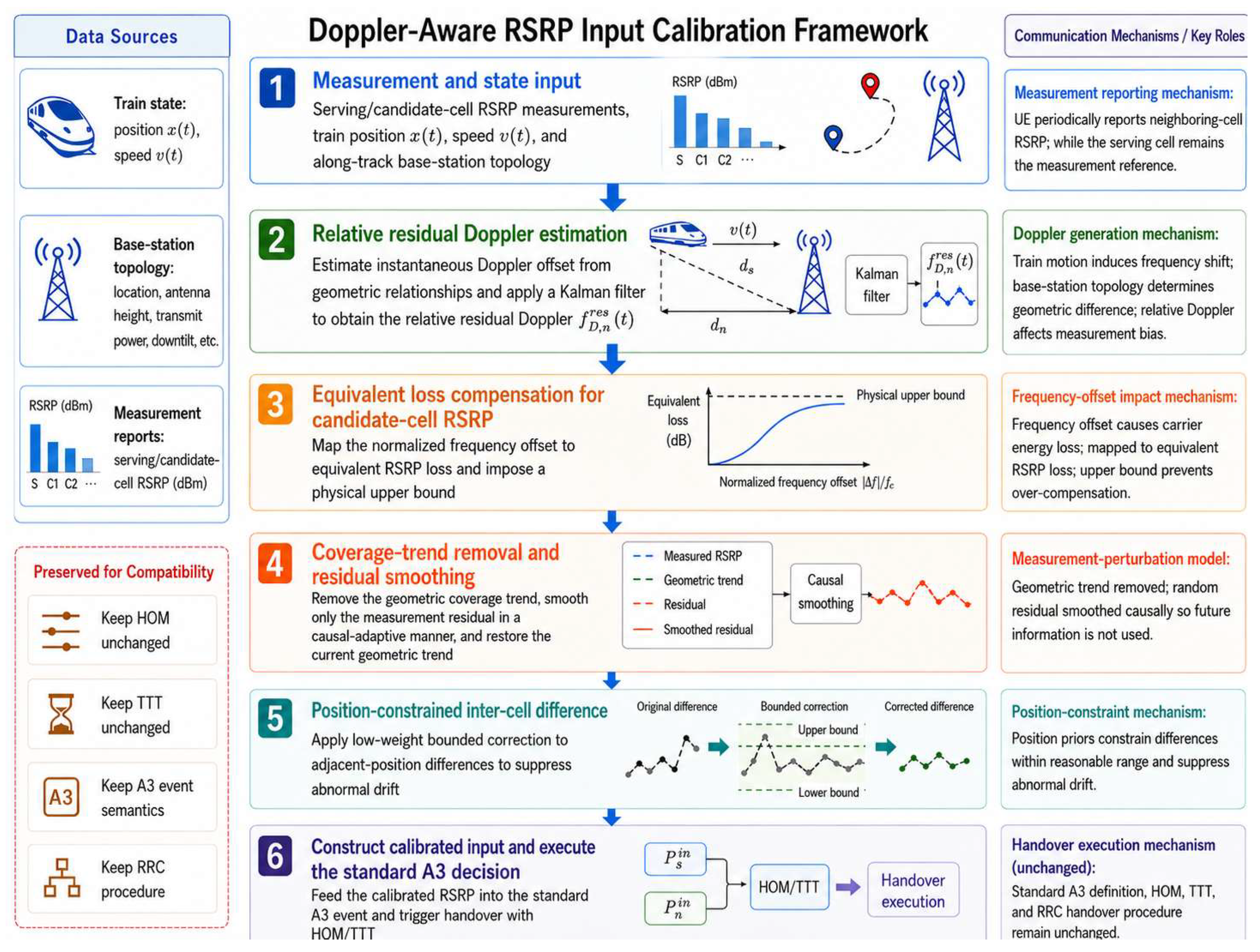
Figure 3.
Comparison of Theoretical Path Loss Between Elevated Bridges and Mountainous Area Scenes.
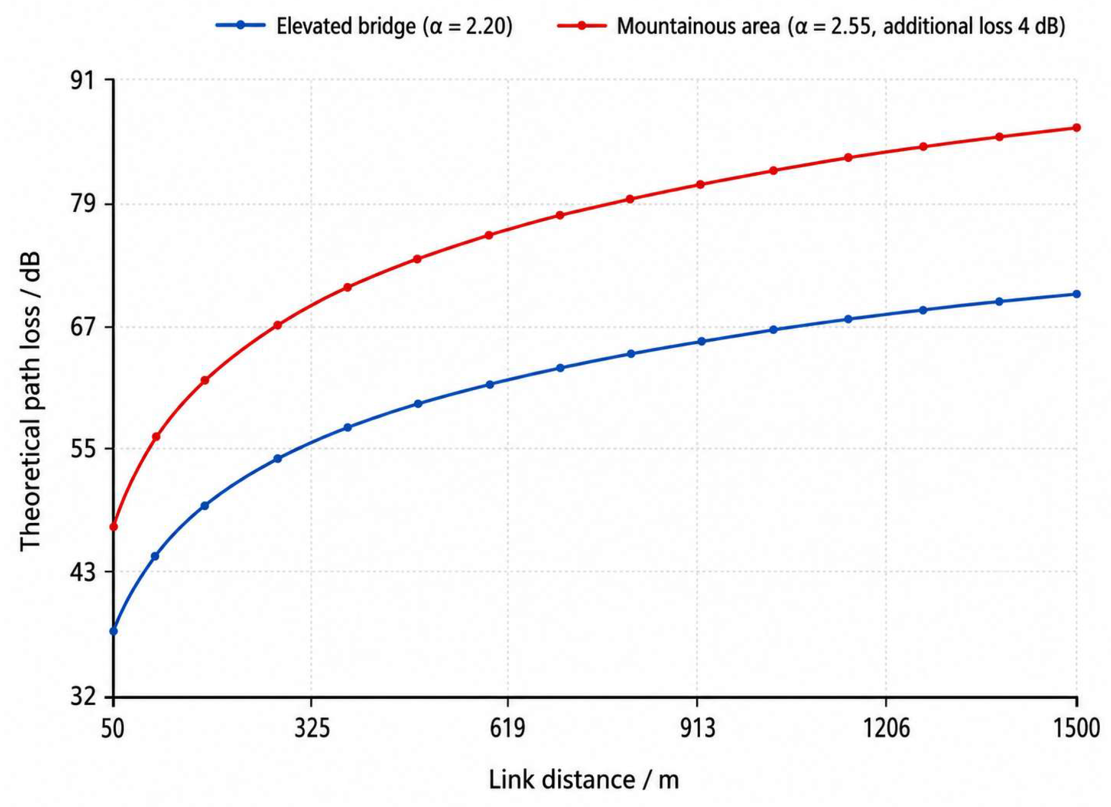
Figure 4.
Relative Residual Doppler Observations and Kalman Estimates.
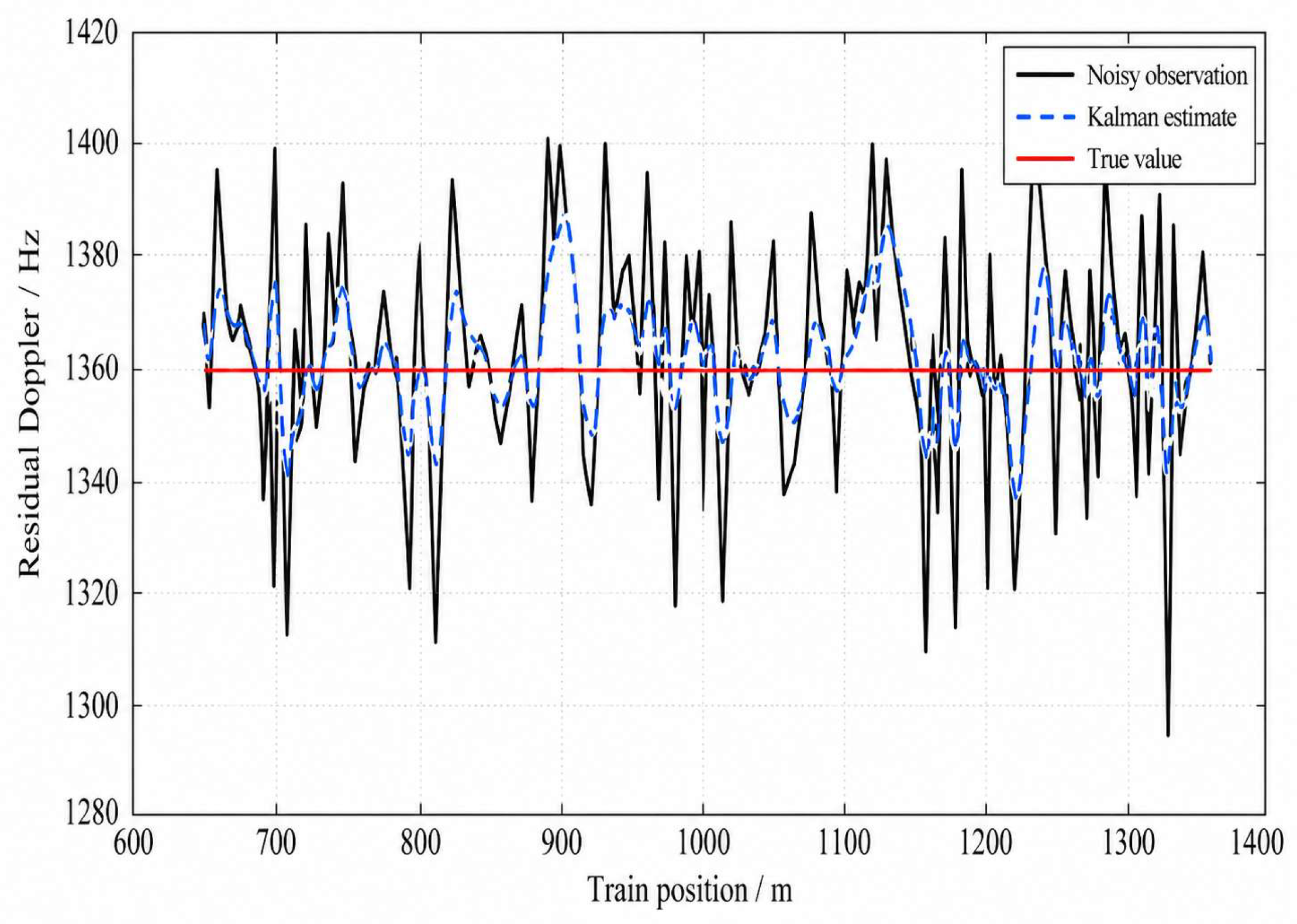
Figure 5.
Stagewise RSRP Calibration Performance of the Proposed Method.
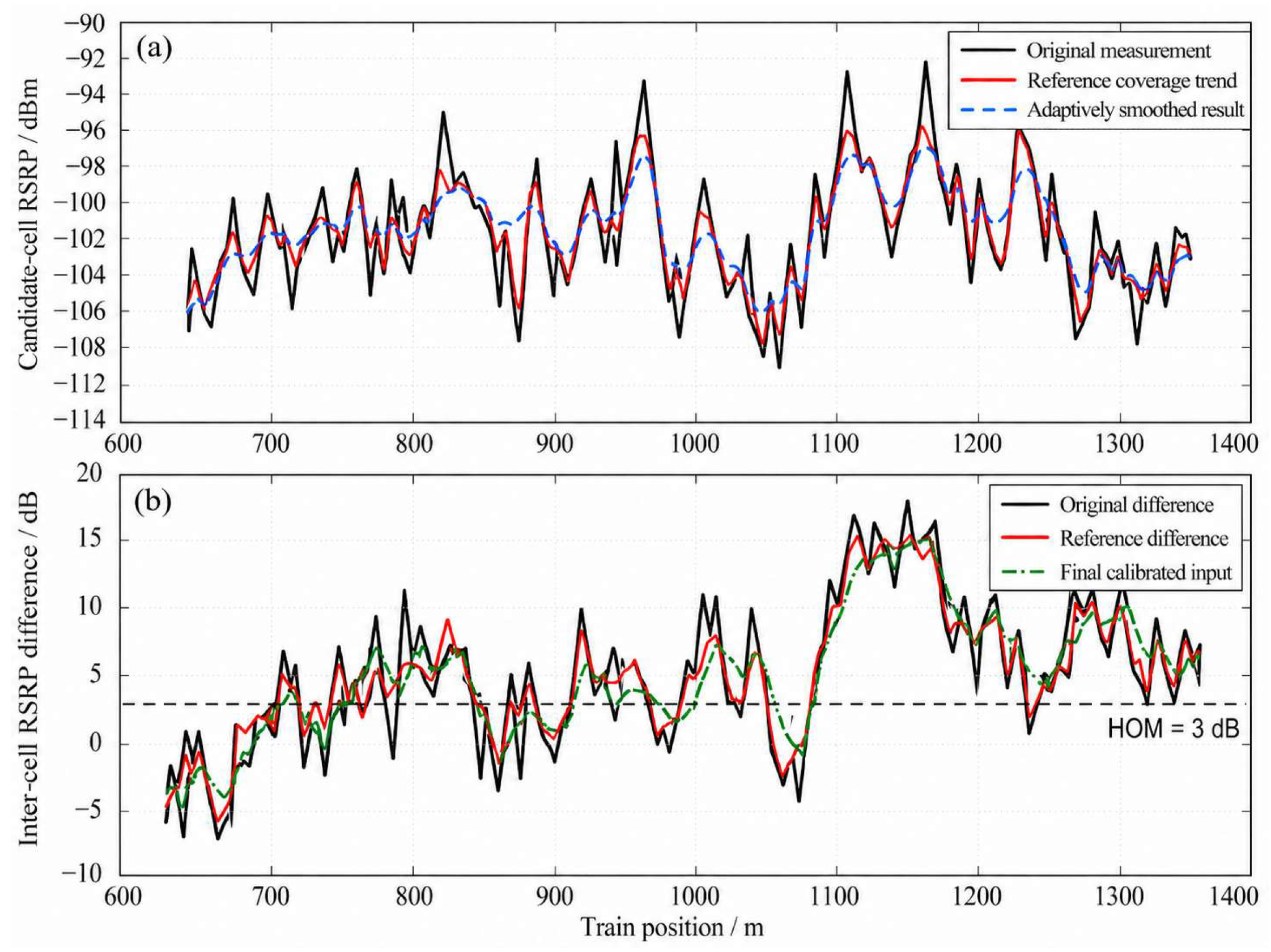
Figure 6.
Theoretical Relationship between Relative Residual Doppler and Equivalent RSRP Loss.
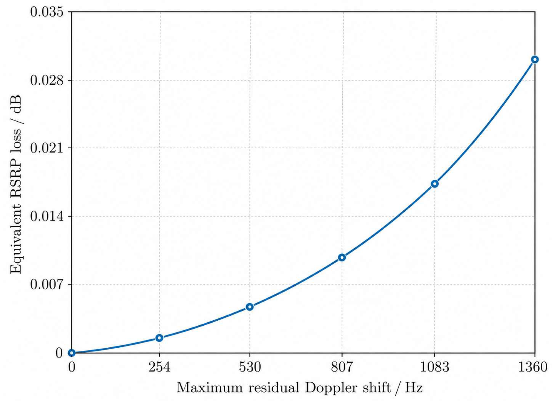
Figure 7.
Handover Success Rates under Different Residual Doppler Ratios.
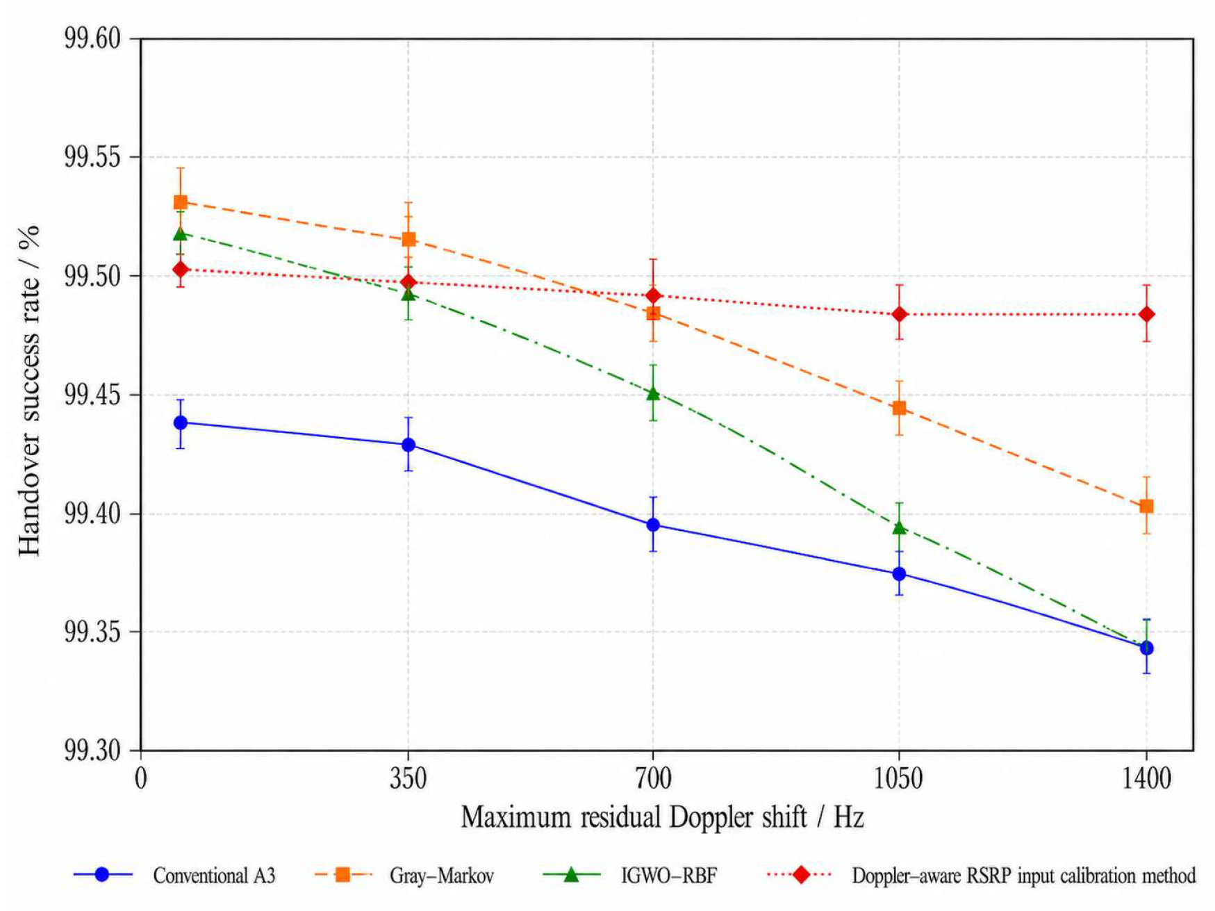
Figure 8.
Trigger Position Errors under Different Residual Doppler Ratios.
Figure 9.
The Handover Success rate and RLF Rate at Different Speeds: (a) Handover Success Rate; (b) RLF Rate.
Figure 9.
The Handover Success rate and RLF Rate at Different Speeds: (a) Handover Success Rate; (b) RLF Rate.
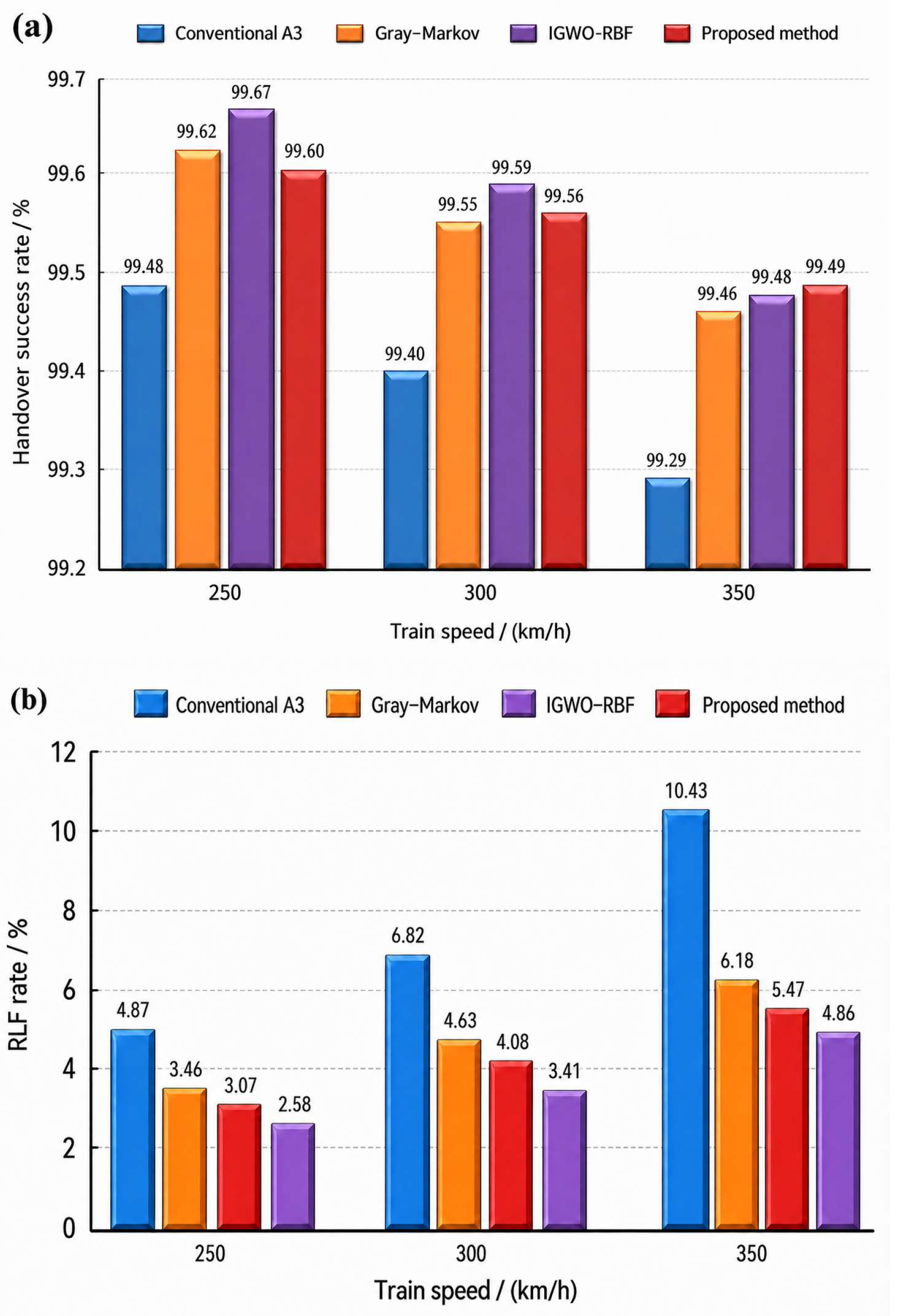
Figure 10.
Ping-Pong Handover Rates at Different Speeds.
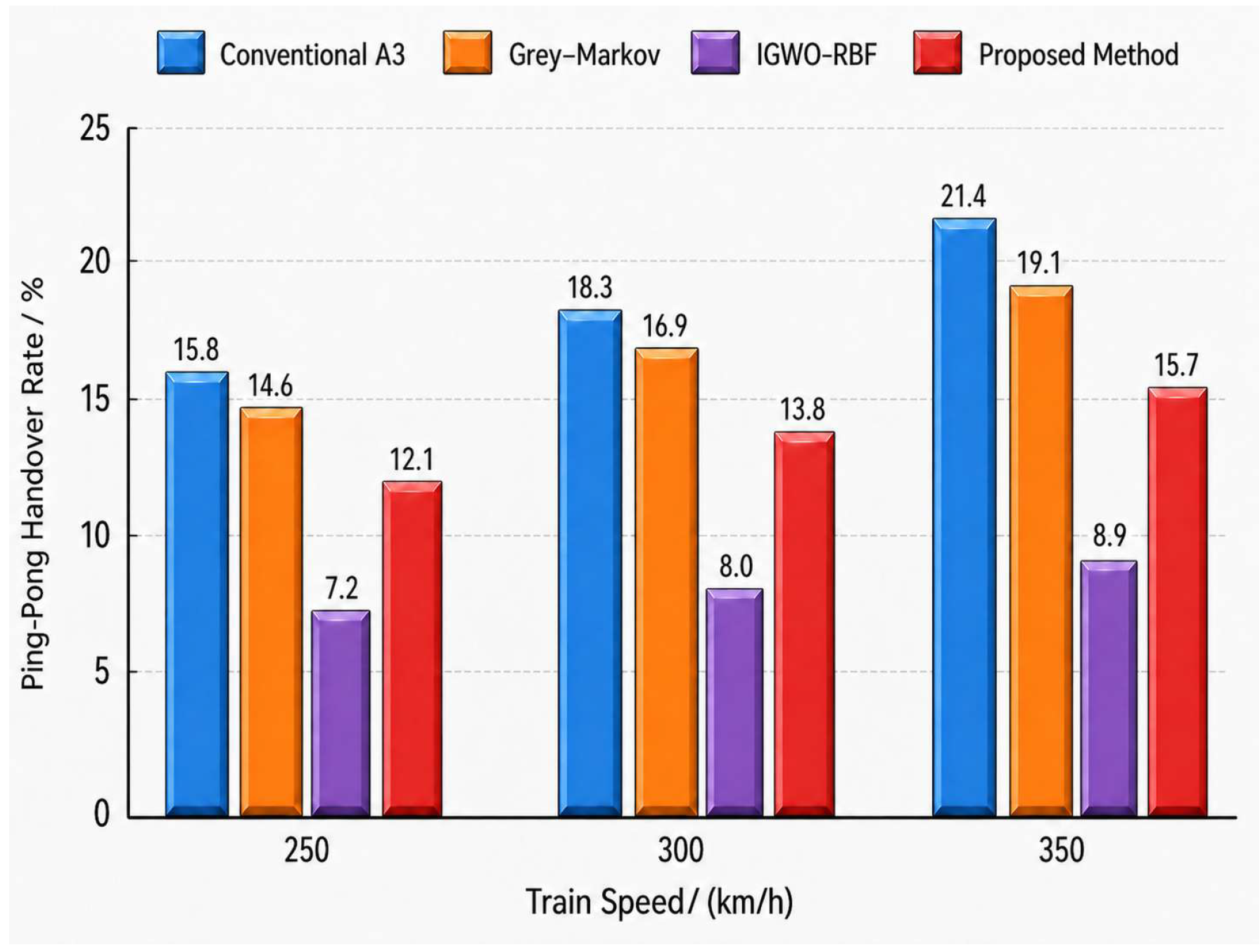
Figure 11.
The Average Trigger Position Error at Different Speeds.
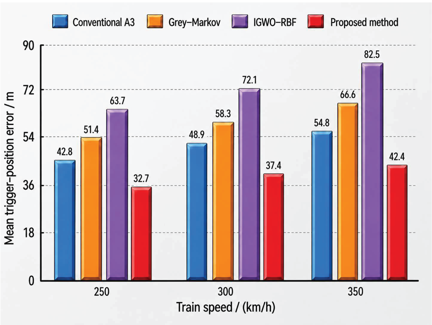
Table 1.
Main Simulation Parameters.
| Parameter | Value | Parameter | Value |
|---|---|---|---|
| Carrier frequency | 2.1 GHz | Subcarrier interval | 30 kHz |
| Base station spacing | 2000 m | Planning radius of the residential area | 1300 m |
| Lateral distance | 35 m | Base station/vehicle-mounted antenna height | 35/3.5 m |
| Train speed | 250、300、350 km/h | Measurement period | 50 ms |
| HOM | 3 dB | TTT | 200 ms |
| Execution time | 100 ms | Ping-Pong Observation window | 3 s |
| Target access threshold | -116.5 dBm | RLF threshold/duration | -120 dBm/100 ms |
| Process noise | 100 Hz2 | Position weight/limit | 0.05/3 dB |
| Number of speed tests | 2000 times per speed | Other test times | 1200 times/condition |
Table 2.
RSRP Root-Mean-Square Errors at Different Processing Stages.
| Processing stage | Candidate cell RSRP RMSE/dB | The difference between cells is RMSE/dB |
| Original measurement | 1.6612 | 2.3449 |
| After Doppler compensation | 1.6609 | 2.3446 |
| After causal adaptive smoothing | 1.5545 | 1.9124 |
| After the position difference is corrected | — | 1.9053 |
Table 3.
Ablation Experiment Results (350 km/h Elevated Bridge Scene).
| Algorithm configuration | Difference RMSE/dB | Trigger position error /m | Success rate /% |
|---|---|---|---|
| Complete algorithm | 1.9053 | 42.35 | 99.44 |
| Remove Doppler compensation | 1.9056 | 43.41 | 99.41 |
| Remove the de-trend processing | 2.0132 | 48.67 | 99.15 |
| Remove position correction | 1.9124 | 44.52 | 99.40 |
Table 5.
Robustness Results in Different Scenarios.
| Scene | Algorithm | Success rate /% | RLF rate /% | Ping-Pong rate /% | Position error /m |
|---|---|---|---|---|---|
| Elevated bridge | Traditional A3 | 99.17 | 15.36 | 19.42 | 49.98 |
| Grey - Markov | 99.50 | 11.89 | 9.97 | 52.25 | |
| IGWO-RBF | 99.47 | 9.47 | 4.31 | 67.23 | |
| The method proposed in this paper | 99.58 | 8.21 | 8.73 | 38.95 | |
| Mountainous area | Traditional A3 | 95.42 | 19.28 | 27.90 | 54.25 |
| Grey - Markov | 95.83 | 16.42 | 24.45 | 63.34 | |
| IGWO-RBF | 96.67 | 11.54 | 15.78 | 78.72 | |
| The method proposed in this paper | 96.05 | 12.77 | 23.53 | 41.98 |
Disclaimer/Publisher’s Note: The statements, opinions and data contained in all publications are solely those of the individual author(s) and contributor(s) and not of MDPI and/or the editor(s). MDPI and/or the editor(s) disclaim responsibility for any injury to people or property resulting from any ideas, methods, instructions or products referred to in the content. |
© 2026 by the authors. Licensee MDPI, Basel, Switzerland. This article is an open access article distributed under the terms and conditions of the Creative Commons Attribution (CC BY) license (http://creativecommons.org/licenses/by/4.0/).
Copyright: This open access article is published under a Creative Commons CC BY 4.0 license, which permit the free download, distribution, and reuse, provided that the author and preprint are cited in any reuse.


