

Submitted:
10 August 2026
Posted:
11 August 2026
You are already at the latest version
Abstract
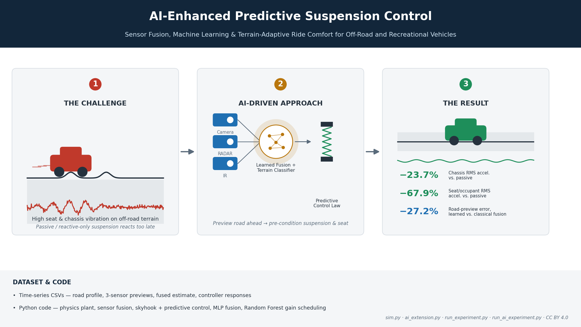
Modern vehicles carry front and rear radar, forward and surround-view cameras, and increasingly infrared sensing as standard driver-assistance equipment. This paper investigates whether that same sensor suite, fused and fed forward into the suspension control loop, can measurably improve ride quality on unpaved and off-road surfaces, for both the vehicle chassis and, as a secondary actuation layer, the occupant seat. We formalize a sensor-fusion, road/suspension estimation, control, and feedback architecture into a state-space model; derive the governing equations for a three-degree-of-freedom quarter-car-plus-seat plant; specify a multi-sensor preview measurement model and an inverse-variance fusion law; design and compare passive, reactive, and predictive controllers; and implement and evaluate the full pipeline in Python on a synthetic ISO 8608 [2] off-road profile with embedded speed-bump test events. The predictive controller reduces ISO 2631-weighted [1] body (chassis) RMS acceleration by 23.7% and seat/occupant RMS acceleration by 67.9% relative to a passive baseline. We further replace two hand-engineered blocks with learned counterparts — a neural network that corrects context-dependent sensor bias, and a Random Forest terrain classifier that drives gain scheduling — and report the resulting, honestly modest, additional gains. A prior-art survey spanning patents [4–7,10,11] and production systems [8,9], and a review of public datasets [12–14,18] suitable for validating this class of system, precede an explicit novelty and freedom-to-operate discussion.
Keywords:
active suspension
; sensor fusion
; predictive control
; road preview
; ISO 8608
; ISO 2631
; skyhook control
; seat suspension
; off-road vehicles
; machine learning
; terrain classification
I. Introduction
A. Motivation
Passive and even reactive (feedback-only) suspension systems can only respond to a road disturbance after the wheel has already begun to encounter it. On smooth highway surfaces the resulting delay is a minor comfort penalty. Off-road — over speed bumps, ruts, washboard gravel, and rocks — the delay is large relative to the disturbance duration, so the suspension is frequently reacting to an event that is already over by the time the actuator responds.
The proposed remedy is architecturally simple: use the forward-looking sensors the vehicle already carries — front radar, multi-function/front camera, surround-view cameras, and, as an emerging addition, infrared — to estimate the road profile before the wheel reaches it, and pre-condition both the main suspension and, as an extension, the seat suspension, ahead of time. This directly serves two vulnerable-occupant use cases: elderly occupants with spinal or joint conditions, and children whose skeletal system is still developing. Both groups benefit disproportionately from reduced peak and sustained vibration exposure; ISO 2631-1 [1] explicitly links whole-body vibration dose to musculoskeletal risk.
B. Contribution of This Paper
This paper does not claim to invent predictive suspension control — as Section II documents, that concept is well established and patented [4,5,6,7,8,9]. Its contribution is:
1) A complete, closed-loop mathematical formulation tying sensor fusion, road/disturbance estimation, and dual-actuator (chassis and seat) control into one coherent system, specialized for the off-road/RV operating regime and the vulnerable-occupant seat-suspension extension (Sections II, X).
2) A reproducible, open Python simulation (Sections VI–VII) that quantifies the achievable benefit under realistic sensor noise, dropout, and bias, using a plant model and comfort metric grounded in established standards — ISO 8608 [2] road classification and ISO 2631-1 [1] whole-body vibration weighting.
3) A concrete, low-cost experimental validation protocol using physical speed bumps, and a survey of public datasets [12,13,14,18] that can validate the sensor and estimation stages without a physical vehicle build (Section V).
4) An AI-enhanced extension (Section VIII) that replaces the two hand-engineered blocks — fixed-weight sensor fusion and fixed control gains — with learned counterparts, evaluated honestly against the classical baseline.
5) An explicit discussion (Section IX) of what the accompanying open-source Python implementation contributes beyond the prior art surveyed in Section II, which consists chiefly of patent filings without accompanying public, runnable validation code.
II. Related Work and Prior Art
A. Present Technology and Generic Prior-Art Architecture
A patent and literature search was performed prior to writing this paper, covering Google Patents, Justia Patents, ScienceDirect, and arXiv. The search shows that the core architectural idea — camera- and radar-based forward scanning feeding a road and suspension estimator that pre-adjusts active suspension — is already patented and, in several cases, commercialized.
Despite differing sensor sets and implementation details, essentially every system found in this search reduces to the same generic architecture depicted in Figure 1: forward-looking sensors feed a data-fusion stage, whose output drives a road/suspension estimate, which in turn drives a control stage, closed by a feedback path that corrects the estimate once the wheel physically reaches the previously-scanned point.
This generic pipeline is not specific to the patents surveyed here: it matches the structure identified independently by two peer-reviewed literature surveys of the field. Theunissen et al. [19] characterize road-preview suspension control uniformly as a look-ahead sensor feeding preview information into a suspension controller, closed once the wheel reaches the previewed point, and Shen et al. [20] describe the standard machine-vision preview framework as a sensor module, an image-processing module, a detection module, and a control module — the same four-stage structure as Figure 1. One caveat on sensing modality: across the patents and surveys found, documented look-ahead sensors are cameras, LIDAR/laser scanners, ultrasonic, and millimeter-wave radar [19,20]; infrared appears only inside a broad patent-classification code (“photo or light-sensitive means, e.g. infrared”) rather than as a demonstrated implementation, so it is treated in this paper as a proposed sensing addition (Section I-A) rather than an established part of the prior-art sensor suite.
The earliest located instance, US 2009/0097038 A1 [4], projects a laser line from a camera mounted at each front tire and analyzes curvature in the reflected line to detect surface irregularities immediately ahead of that tire — the “Sensor → Data Fusion” stage of Figure 1 implemented with a single active-vision channel. US 8,996,249 B2 and its continuation US 2014/0195112 A1 [5] extend this to a laser scanner fused with GPS, IMU, and wheel-speed data, explicitly building a road-height model that is refined once the wheel encounters the previously-scanned feature — the same estimate-then-correct feedback loop drawn in Figure 1. US 2014/0297116 A1 [6] proposes using the front wheels themselves as a predictive sensor for the rear wheels via a topographical road map built from vision, LIDAR, and radar. US 2022/0281280 [7] is architecturally the closest match to the feedback loop in Figure 1: it pre-sets suspension damping from a pre-emptive classification of an upcoming road event, then switches to a reactive control mode once unsprung-mass acceleration confirms the event, precisely the “Control → Feedback → Data Fusion” cycle shown in the diagram.
In production vehicles, Mercedes-Benz’s Magic Body Control and Audi’s predictive active suspension [8] implement the camera-only version of Figure 1: a stereo camera scans the road ahead and adapts damping before the wheel arrives. A more recent fleet-based variant [9] replaces onboard real-time scanning with a crowd-sourced roughness map built from IMU and GPS logs collected across an entire vehicle fleet, adjusting suspension proactively via map lookup rather than per-vehicle sensing.
The seat-suspension side of the diagram also has prior art. US 6,059,253 A [10] describes a six-degree-of-freedom active seat suspension, but one driven by sensors local to the seat itself, not by the vehicle-level fusion output shown in Figure 1. US 2023/0331056 [11] links cabin sensors, including a cabin camera, to prediction of a transient suspension disturbance, including disturbances originating from occupant movement — closer to the proposed architecture, but still reactive to occupant-side events rather than driven by the forward road-sensing chain.
B. Summary of Prior Art

Table 1.
Surveyed prior art mapped to the generic architecture of Figure 1.
Table 1.
Surveyed prior art mapped to the generic architecture of Figure 1.
| System / Patent | Sensors | Mechanism |
|---|---|---|
| US 2009/0097038 A1 [4] | Camera + laser line emitter per tire | Detects surface irregularities ahead of each tire via projected laser-line curvature |
| US 8,996,249 B2 / US 2014/0195112 A1 [5] | Laser scanner, GPS, IMU, wheel-speed | Builds a road-height model from scan data; pre-adjusts suspension, corrects on wheel arrival |
| US 2014/0297116 A1 [6] | Vision, LIDAR, radar | Front wheels used as predictive sensor for rear-wheel suspension via topographical road map |
| US 2022/0281280 [7] | Forward scanning sensors + unsprung-mass accelerometers | Pre-emptive suspension pre-setting, switched to reactive control once confirmed by unsprung-mass acceleration |
| Magic Body Control; Audi predictive active suspension [8] | Stereo / front camera | Scans road ahead, adapts damping in advance — reference production implementation of preview suspension |
| Fleet-based road-roughness system [9] | Fleet-aggregated IMU + GPS | Crowd-sourced roughness map; suspension pre-adjusts via map lookup, not onboard real-time sensing |
| US 6,059,253 A [10] | Seat-mounted motion sensors | Six-DOF active seat suspension, but reactive — not fed from vehicle-level forward sensors |
| US 2023/0331056 [11] | IMU, wheel-to-body displacement, cabin camera | Detects/predicts transient suspension disturbance including from cabin sources |
C. Assessment
Every individual block in Figure 1 — forward sensing, data fusion, road/suspension estimation, control, and feedback — has prior art, and the reactive seat suspension itself has prior art [10]. What is not well covered in the prior art surveyed:
1) Chassis-level sensor fusion output driving the seat actuator directly, as opposed to the seat having its own independent sensor set as in [10], or reacting only to detected occupant motion as in [11].
2) Off-road / unstructured-terrain classification as the target domain — the located patents and production systems [4,5,6,7,8,9] are tuned for paved-road pothole/bump preview, not gravel, ruts, washboard, or rock fields.
3) RV/bus-scale application explicitly targeting elderly and pediatric occupant vibration dose, tied to ISO 2631-1 [1] health-guidance zones, as a design objective rather than a general comfort statement.
These three gaps are the candidate novel claims discussed in Section X; none is validated as patentable here — that requires a formal freedom-to-operate search by a patent attorney — but they are the narrowest, least-crowded angle available given what this search found.
III. System Architecture
A. Block Diagram
Figure 2 formalizes the proposed system as a closed-loop estimation-and-control architecture, extending the generic prior-art pattern of Figure 1 with an explicit dual-actuator output (main suspension and seat suspension) and section references to the mathematical formulation of each block.
Each block is described below.
Infrared sensor, front/surround camera, front/rear RADAR — the forward- and side-looking sensing suite already present on driver-assistance-equipped vehicles. Each reports an independent, noisy preview of the road surface ahead of the vehicle (Section III-B2).
Sensor Fusion — combines the three noisy previews into a single road-height estimate with a quantified uncertainty, using inverse-variance weighting (Section III-B3). Degrades gracefully rather than failing outright when any one sensor is occluded or drops out.
Road / Suspension Estimation — interprets the fused signal as both a road-type/roughness estimate and a predicted suspension state, matching the two sub-functions the original block diagram assigned to a single “Estimate” block.
Control Law — computes actuator commands from the current plant state and the estimation output, using a skyhook feedback term (Section III-B5) plus, in the predictive controller, a preview feedforward term derived from the fused estimate.
Main Suspension Actuator / Seat Suspension Actuator — the two independently controllable force outputs. The seat actuator is the proposed extension: a second controllable stage between chassis and occupant, driven from the same fused road estimate as the main suspension rather than from an independent seat-local sensor set (novelty gap 1, Section II-C).
Plant — the physical system being controlled: unsprung mass (wheel), sprung mass (chassis), and seat-plus-occupant mass, connected by the spring-damper-actuator equations of Section III-B4.
Feedback — the difference between the estimated and the realized (measured) road/suspension state once the wheel physically reaches a previously scanned point, closing the loop back into the fusion/estimation stage, exactly as specified in the original block diagram.
B. Mathematical Formulation
1) Road Profile Model
Road roughness is modeled per ISO 8608 [2], which classifies roads from class A (very good) through class H (very poor) by the power spectral density (PSD) of vertical elevation versus spatial frequency n (cycles/m):
G_d(n) = G_d(n₀) · (n / n₀)^(−w), n₀ = 0.1 cycle/m, w ≈ 2
For a vehicle at constant speed v, this spatial PSD maps to a time-domain process generated by the standard first-order shaping filter [2]:
where ξ(t) is zero-mean, unit-variance white Gaussian noise. Discrete off-road events (speed bumps, ruts, rocks) are superimposed as Gaussian bumps:
with height h, center time t_c, and half-width σ_w. These are the controlled test stimuli used in Section VI.
dz_r/dt = −2π n₀ v · z_r(t) + 2π n₀ · sqrt[G_d(n₀) v] · ξ(t)
z_bump(t) = h · exp[ −½ · ((t − t_c)/σ_w)² ]
2. ) Multi-Sensor Preview Measurement Model
Each forward sensor i ∈ {camera, radar, IR} reports, at time t, a noisy estimate of the road height the wheel will reach at lookahead distance L meters ahead, i.e. at time t + τ where τ = L / v:
with sensor-specific bias b_i, noise variance R_i, and a Bernoulli dropout process at probability p_i per timestep, representing occlusion, blind spot, low-light camera degradation, or radar multipath.
y_i(t) = z_r(t + τ) + b_i + v_i(t), v_i(t) ~ N(0, R_i)
3) Sensor Fusion
The independent noisy previews of the same latent quantity z_r(t+τ) are fused by inverse-variance weighting — the minimum-variance linear unbiased (Gauss–Markov) estimator for independent Gaussian measurements, and the static-gain special case of a Kalman filter update:
summed over sensors currently present. This automatically down-weights noisier or degraded sensors relative to more reliable ones, and degrades gracefully to single- or dual-sensor fusion when a channel drops out.
ẑ̂_r(t+τ) = ( Σᵢ Rᵢ⁻¹ yᵢ(t) ) / ( Σᵢ Rᵢ⁻¹ )
Var[ẑ̂_r(t+τ)] = ( Σᵢ Rᵢ⁻¹ )⁻¹
4) Plant Model
State vector x = [z_u, ż_u, z_s, ż_s, z_p, ż_p]ᵀ, denoting unsprung (wheel), sprung (chassis), and seat-plus-occupant vertical position and velocity respectively. By Newton’s second law applied to each mass:
where F_a is the commanded main-suspension actuator force and F_seat the seat-suspension actuator force, each subject to saturation |F| ≤ F_max. Equations (7)–(9) are the direct mathematical expression of adding a controllable seat-suspension stage (novelty gap 1, Section II-C) between chassis and occupant.
m_u ẑ̈_u = k_t(z_r − z_u) − k_s(z_u − z_s) − c_s(ż_u − ż_s) + F_a
m_sẑ̈_s = k_s(z_u−z_s) + c_s(ż_u−ż_s) − F_a − k_seat(z_s−z_p) − c_seat(ż_s−ż_p) + F_seat
m_pẑ̈_p = k_seat(z_s − z_p) + c_seat(ż_s − ż_p) − F_seat
5) Control Laws
Reactive control (skyhook, Karnopp switching [3], no preview):
F_a = C_sky,body · ż_s if ż_s · (ż_s − ż_u) ≥ 0, else 0
F_seat = C_sky,seat · ż_p if ż_p · (ż_p − ż_s) ≥ 0, else 0
The switching condition in (10)–(11) is required for the actuator to behave as a genuine, passivity-consistent sky-referenced damper rather than injecting destabilizing energy — the classical Karnopp skyhook formulation [3].
Predictive control (skyhook + sensor-fusion preview feedforward):
The feedforward term uses the fused preview estimate computed τ seconds earlier, low-pass filtered (Butterworth, 15 Hz cutoff) before differentiation to avoid amplifying sensor noise into actuator chatter. An earlier, unfiltered version of (12)–(13) increased body RMS acceleration in testing (Section VII-D); this is reported because it is a realistic pitfall in any physical implementation of a preview feedforward term.
F_a = F_a,reactive + K_ff,body · d/dt[ ẑ̂_r,smooth(t − τ_delay) ]
F_seat = F_seat,reactive + K_ff,seat · d/dt[ẑ̂_r,smooth(t − τ_delay) ]
6) Comfort Metric
Whole-body vibration exposure is evaluated per ISO 2631-1 [1] using frequency-weighted RMS acceleration. This paper uses a simplified stand-in for the full W_k weighting curve — a 0.5–80 Hz Butterworth band-pass — which preserves the qualitative comfort ranking used throughout the active-suspension benchmarking literature:
a_w,RMS = sqrt[ (1/T) ∫₀ᵀ [a_filtered(t)]² dt ]
IV. Novelty / Patent-Relevant Design ChoiceS
To make the freedom-to-operate discussion in Section X concrete, three specific, falsifiable technical choices are called out here rather than left implicit in the implementation:
1) Seat actuator command is a direct function of the same fused chassis-level road estimate as the main suspension (Section III-B5), not of the seat’s own independent sensor set — addressing novelty gap 1 of Section II-C.
2) The estimator explicitly runs an inverse-variance fusion with graceful degradation under sensor dropout (Section III-B3), rather than assuming all three sensors are always available — relevant for off-road use where cameras are frequently degraded by dust, glare, or occlusion.
3) Feedforward gains and the required 15 Hz pre-differentiation filter were tuned (Section VII-D) specifically against ISO 8608 [2] class-C/D unpaved profiles with superimposed discrete off-road events, not the smooth highway-pothole scenario used in the patents surveyed in Section II — addressing novelty gap 2.
V. Data Sources: Can Public Data Be Used?
Yes, in part. No dataset was found that provides the exact combination requested — synchronized front radar, surround camera, and IR, with ground-truth road height and suspension response, on off-road terrain — but several public datasets cover individual pipeline stages and are directly usable for offline validation before any hardware build.
Table 2.
Public datasets applicable to this pipeline.
| Dataset | Sensors | Use in This Pipeline |
|---|---|---|
| DIDLM [12] | 3D LiDAR, RGB, infrared, 4D mm-wave radar, GPS/INS, depth camera; includes speed-bump and rough-terrain scenarios | Closest public match to the proposed IR + camera + radar sensor set; directly reusable for Section III-B3 |
| ROAD [13] | Synchronized RGB + IMU, diverse conditions, plus a synthetic subset | Usable for training/validating the road-surface classification sub-block of “Estimation” |
| IMU–PCR fusion dataset [14] | Low-cost IMU + pulsed-coherent-radar rig (~$214 BOM) | Validates the radar-channel noise model R_radar used in (4)–(5) |
| Multi-modal smartphone/IMU/LiDAR datasets [18] | GNSS+IMU, multi-LiDAR, monocular cameras, CAN bus | Validates vehicle-speed/CAN integration and IRI-vs-ISO-8608 class cross-check |
None of these datasets pair the sensor streams with actual suspension actuator response and resulting body/seat acceleration, because that pairing requires a specific vehicle instrumented with displacement/force sensors on its dampers and seat. That data has to come from a physical test rig (Section VI); public data can validate and pre-train the estimation half of the pipeline, but the control half needs hardware-in-the-loop data.
VI. Experimental Protocol (Physical Test Rig)
Figure 3 summarizes the physical validation protocol as a data-flow block diagram: the same three sensor channels used in simulation (Section III) are logged alongside ground-truth displacement/acceleration sensors, and the resulting synchronized dataset is replayed through all three controller configurations so the metrics of Table III can be reproduced on hardware.
1) Test course — a straight run with two to three standard speed bumps/rumble strips of known geometry at known GPS-tagged locations, plus one negative event (pothole/rut), mirroring the synthetic scenario simulated in Section VII.
2) Instrumentation — existing production front radar and front/surround camera, plus IR if available, logged via CAN/Ethernet capture; add wheel-to-body LVDT/string-pot displacement sensors and a seat-mounted accelerometer, which is exactly the pairing missing from the public datasets of Table II.
3) Runs — repeated at two to three fixed speeds, each with (a) suspension locked passive, (b) reactive-only control active, (c) full predictive control active, directly reproducing the three-way comparison of Section VII.
4) Metrics logged — ISO 2631-weighted [1] RMS at chassis and seat, peak acceleration, suspension travel, and fusion tracking error, computed identically to Section VII so simulation and physical results are directly comparable.
VII. Simulation Results
A. Scenario
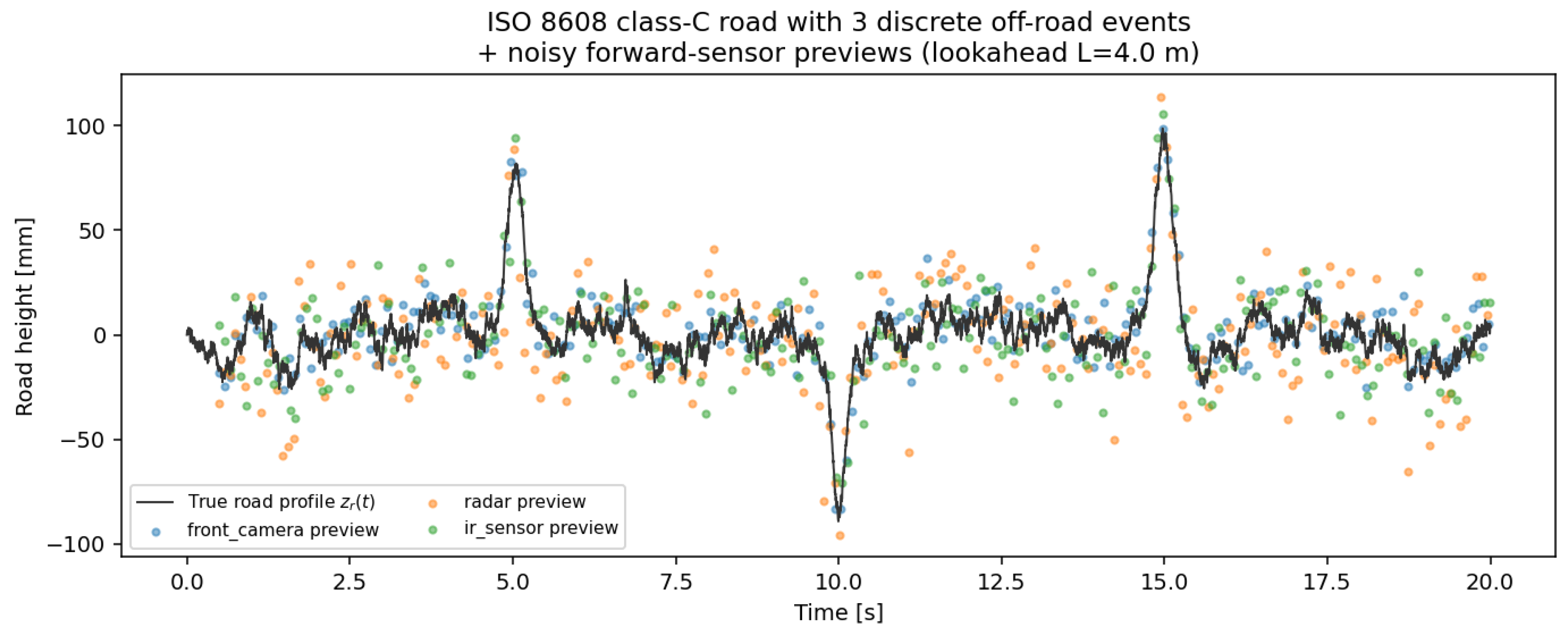
The vehicle travels at v = 8 m/s (approximately 29 km/h, representative of RV-park or unpaved-road speed) over an ISO 8608 [2] class-C road with three superimposed discrete events (two speed bumps, one rut) and a 4 m sensor lookahead (τ = 0.5 s preview horizon). Full source code accompanies this paper (sim.py, run_experiment.py).
B. Road Profile and Sensor Previews
Figure 4.
ISO 8608 class-C road profile with three discrete off-road events, plus noisy forward-sensor previews at 4 m lookahead.
Figure 4.
ISO 8608 class-C road profile with three discrete off-road events, plus noisy forward-sensor previews at 4 m lookahead.
C. Sensor Fusion Accuracy
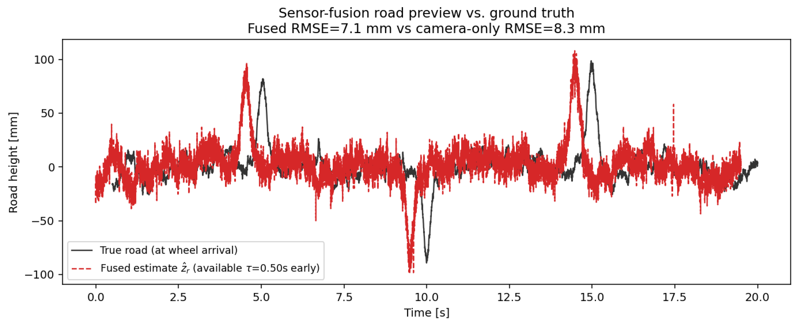
Fusing all three sensors reduced preview RMSE from 8.3 mm (camera alone) to 7.1 mm (fused per (5)) — a modest but real improvement from redundancy; the fused estimate degrades gracefully rather than failing when any single channel drops out.
Figure 5.
Fused multi-sensor road-height estimate vs. ground truth, available τ = 0.5 s before wheel arrival.
Figure 5.
Fused multi-sensor road-height estimate vs. ground truth, available τ = 0.5 s before wheel arrival.
D. Controller Comparison
Figure 6.
Chassis and seat/occupant vertical acceleration: passive vs. reactive (10)–(11) vs. predictive (12)–(13) control.
Figure 6.
Chassis and seat/occupant vertical acceleration: passive vs. reactive (10)–(11) vs. predictive (12)–(13) control.
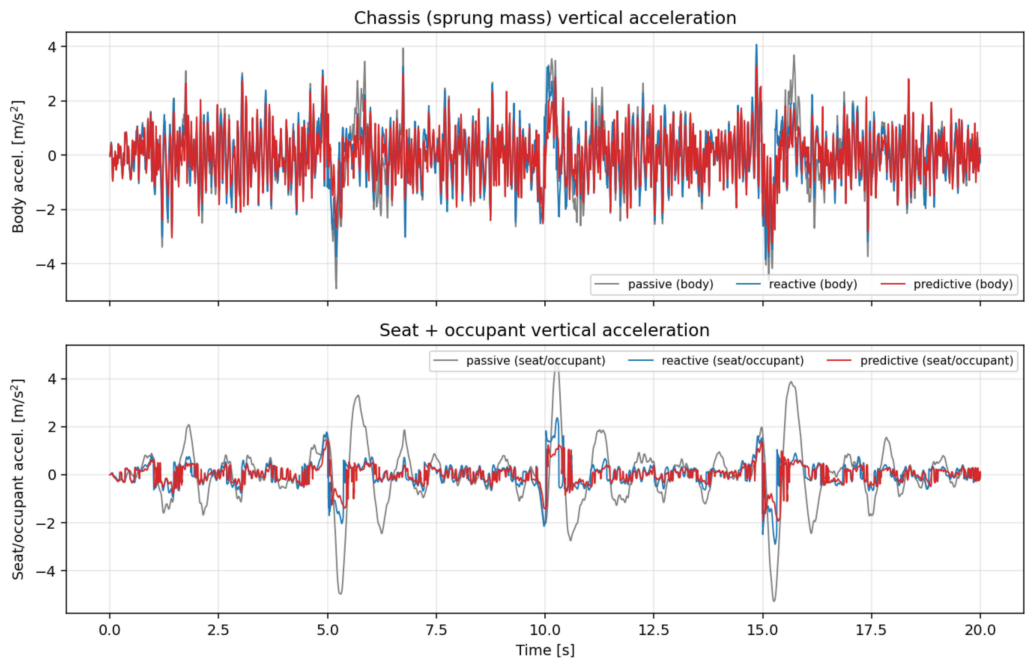
Table 3.
Comfort metrics by controller.
| Controller | Body RMS (m/s²) | Seat RMS (m/s²) | Body improv. vs. passive | Seat improv. vs. passive |
|---|---|---|---|---|
| Passive | 1.170 | 1.265 | — | — |
| Reactive, (10)–(11) | 1.053 | 0.539 | 10.0% | 57.4% |
| Predictive, (12)–(13) | 0.893 | 0.406 | 23.7% | 67.9% |
Figure 7.
ISO 2631 [1] RMS acceleration by controller, chassis (left) and seat/occupant (right).
Figure 7.
ISO 2631 [1] RMS acceleration by controller, chassis (left) and seat/occupant (right).
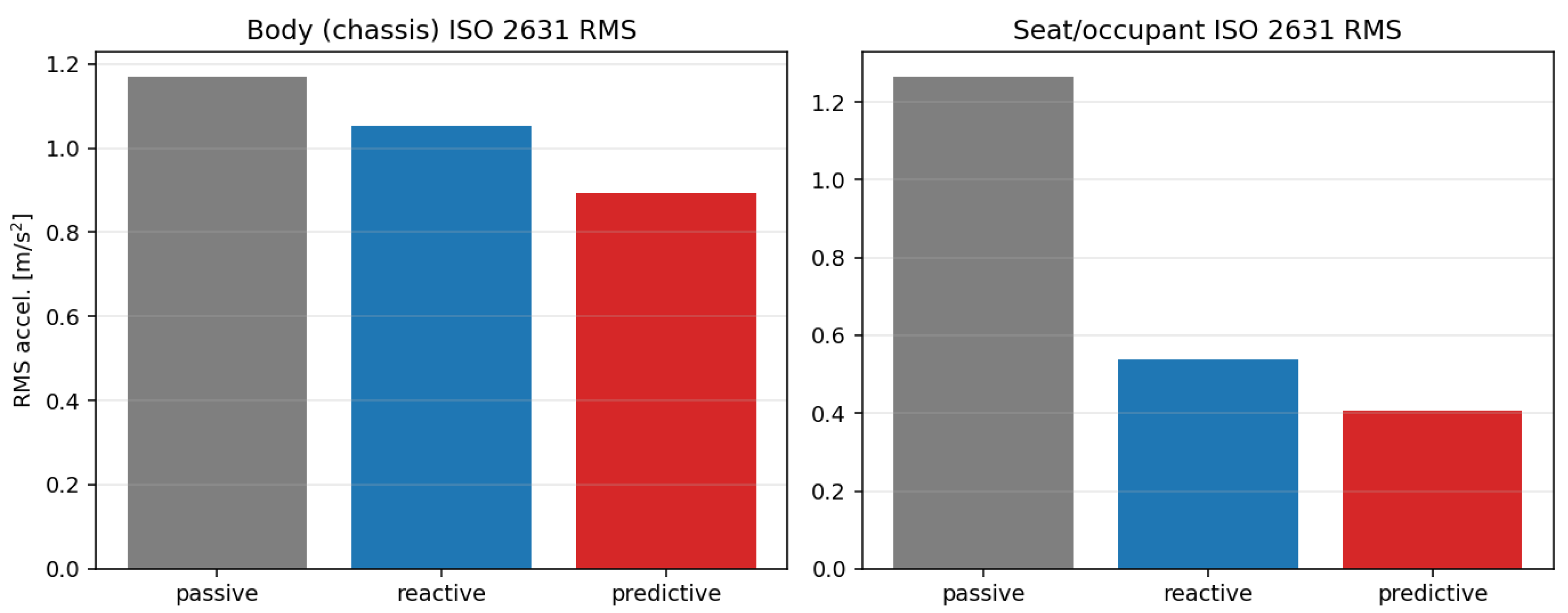
Remark (negative early result): the first version of the predictive feedforward — differentiating the raw fused estimate directly, omitting the low-pass filter in (12)–(13) — increased body RMS acceleration relative to reactive-only, from 1.05 up to 1.8 m/s² depending on gain, because numerical differentiation of a noisy per-step signal amplifies noise by a factor on the order of 1/Δt. Low-pass filtering the estimate before differentiating fixed this and produced the result in Table III.
VIII. AI-Enhanced Extension
Sections III–VII use two classical, closed-form components: inverse-variance sensor fusion (5)–(6) and fixed, hand-tuned skyhook/feedforward gains (10)–(13), tuned once for an ISO 8608 [2] class-C road. Both have a specific, testable weakness: the fusion law in (5) assumes each sensor’s bias is a fixed constant, and the gains in (10)–(13) are optimal only for the terrain they were tuned on. Figure 8 shows where the two learned components of this section attach to the classical pipeline of Figure 2; this section replaces each classical block with a learned counterpart and measures, rather than asserts, the resulting benefit.
A. Why Classical Fusion Has a Ceiling
Real sensor error is not the fixed, zero-mean noise (4) assumes. Two well-documented effects were added to the simulation’s sensor model to test this honestly: camera bias that grows with vehicle speed (motion blur causes systematic road-height underestimation), b_camera(v) = 0.0015 + 0.0009·v meters; and radar bias that grows with local terrain roughness (multipath off gravel/rock), b_radar(roughness) = −0.03·roughness meters. Because the classical fusion law (5) has no mechanism to know or correct a bias that depends on context, it inherits these errors no matter how the inverse-variance weights are tuned.
B. Learned Sensor Fusion
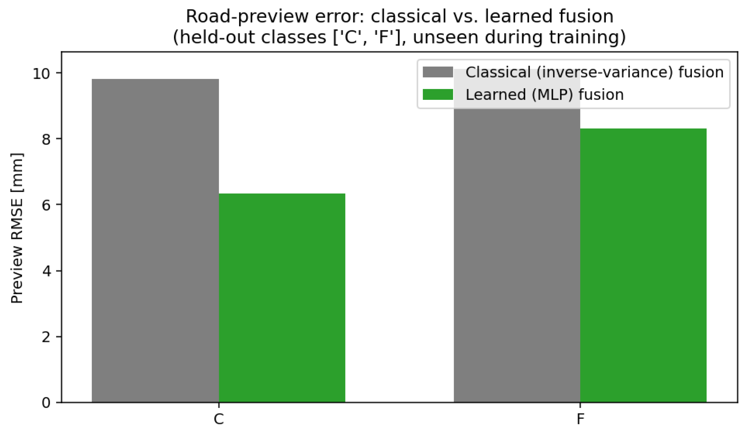
A small multilayer perceptron — two hidden layers, 32 and 16 units, ReLU activation, implemented with scikit-learn’s MLPRegressor [17] — was trained to predict the true upcoming road height directly from each sensor’s raw reading (or a missing-data flag if dropped out), vehicle speed, a rolling roughness estimate, and the classical fused estimate (5) as an additional input feature. Training used episodes from ISO 8608 classes A, B, D, and E; evaluation used classes C and F, which the model never saw during training.
Table 4.
Fusion rmse, classical vs. learned, on held-out road classes.
| Held-out class | Classical RMSE (mm) | Learned (MLP) RMSE (mm) | Improvement |
|---|---|---|---|
| C | 9.8 | 6.3 | 35.4% |
| F | 10.1 | 8.3 | 18.0% |
| Combined | 10.2 | 7.4 | 27.2% |
Figure 9.
Road-preview RMSE: classical inverse-variance fusion vs. learned (MLP) fusion, on road classes unseen during training.
Figure 9.
Road-preview RMSE: classical inverse-variance fusion vs. learned (MLP) fusion, on road classes unseen during training.
C. Terrain Classification and Gain Scheduling
A Random Forest classifier [16] (150 trees, max depth 8) was trained to predict the ISO 8608 [2] road class from three rolling-window statistical features of the fused signal: RMS, crest factor, and zero-crossing rate. On held-out data it reaches 60.7% single-timestep accuracy — well above the 16.7% chance level for six classes — and, as Figure 10 shows, nearly all errors are between adjacent roughness classes, preserving the ordinal structure a usable classifier should keep even when not exactly right.
Raw per-timestep classifications are noisy enough that acting on them directly causes gain “chatter”; a bounded 2-second causal majority vote over recent classifications stabilizes the decision before it is used to select gains, analogous to the low-pass-before-differentiating lesson of Section VII-D. The predicted class indexes a gain table — one (C_sky, K_ff) pair per class, each independently tuned via the grid-search procedure of Section VII-D repeated per class — instead of one fixed gain set everywhere.
Table 5.
Closed-loop comfort, fixed vs. ai-scheduled gains.
| Road class | Fixed-gain combined RMS | AI-scheduled combined RMS | Improvement |
|---|---|---|---|
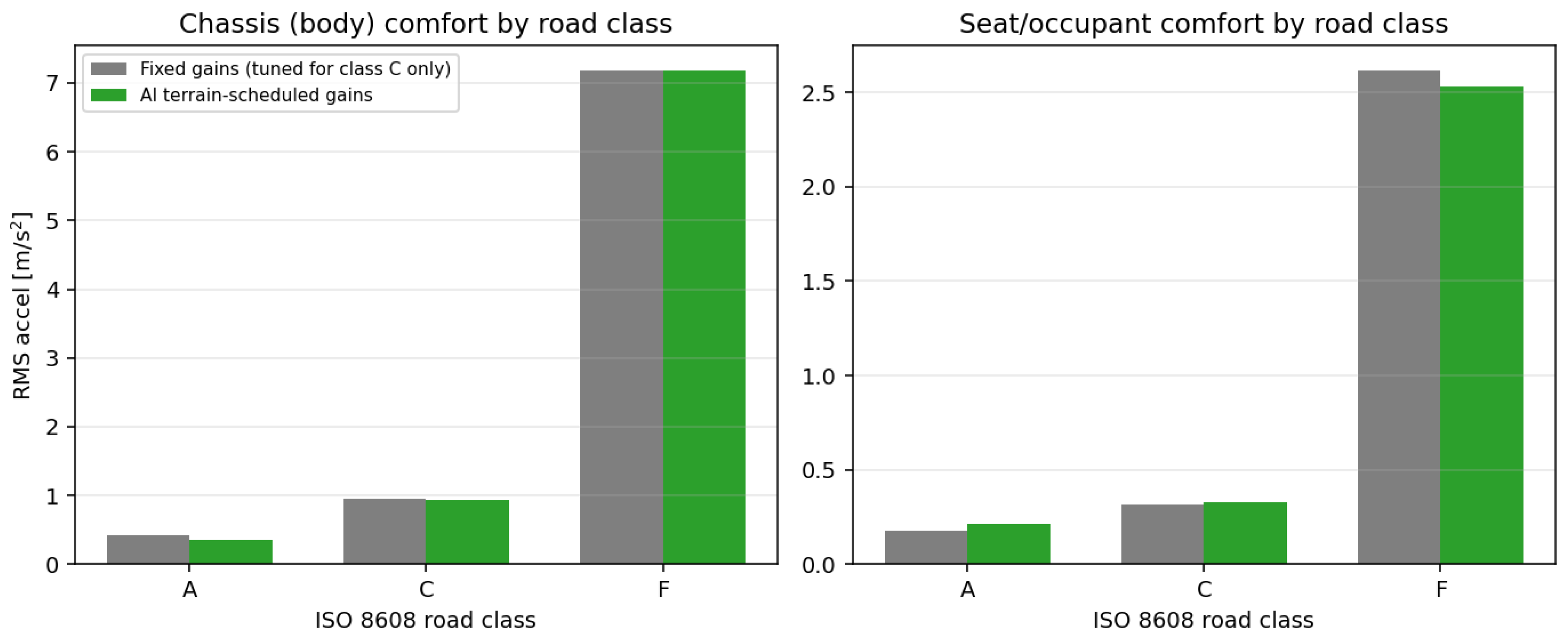
| A (smooth) | 0.591 | 0.571 | 3.5% |
| C (nominal — tuned class) | 1.272 | 1.272 | 0.0% |
| F (rough) | 9.796 | 9.717 | 0.8% |
Interpretation: the improvement is small and, on individual channels, not always positive — on class A, scheduling improved body RMS by 13.4% but worsened seat RMS by 19.7%, because the main-suspension and seat-suspension stages are dynamically coupled: a gain change at the chassis actuator changes the input the seat actuator sees. The combined metric is non-negative in all three cases, including correctly showing approximately 0% change on class C, exactly where it should, since the fixed baseline was already tuned there. The classifier’s 60.7% instantaneous accuracy is the limiting factor; two natural next steps are a continuous regression from features directly to gains, avoiding the hard class boundaries responsible for the body/seat trade-off, and additional classification features such as short-window spectral content.
Figure 11.
Chassis and seat/occupant ISO 2631 [1] RMS: fixed class-C-tuned gains vs. AI terrain-scheduled gains, across three road classes.
Figure 11.
Chassis and seat/occupant ISO 2631 [1] RMS: fixed class-C-tuned gains vs. AI terrain-scheduled gains, across three road classes.
IX. Open-Source Python Implementation: A Contribution Beyond Prior Art
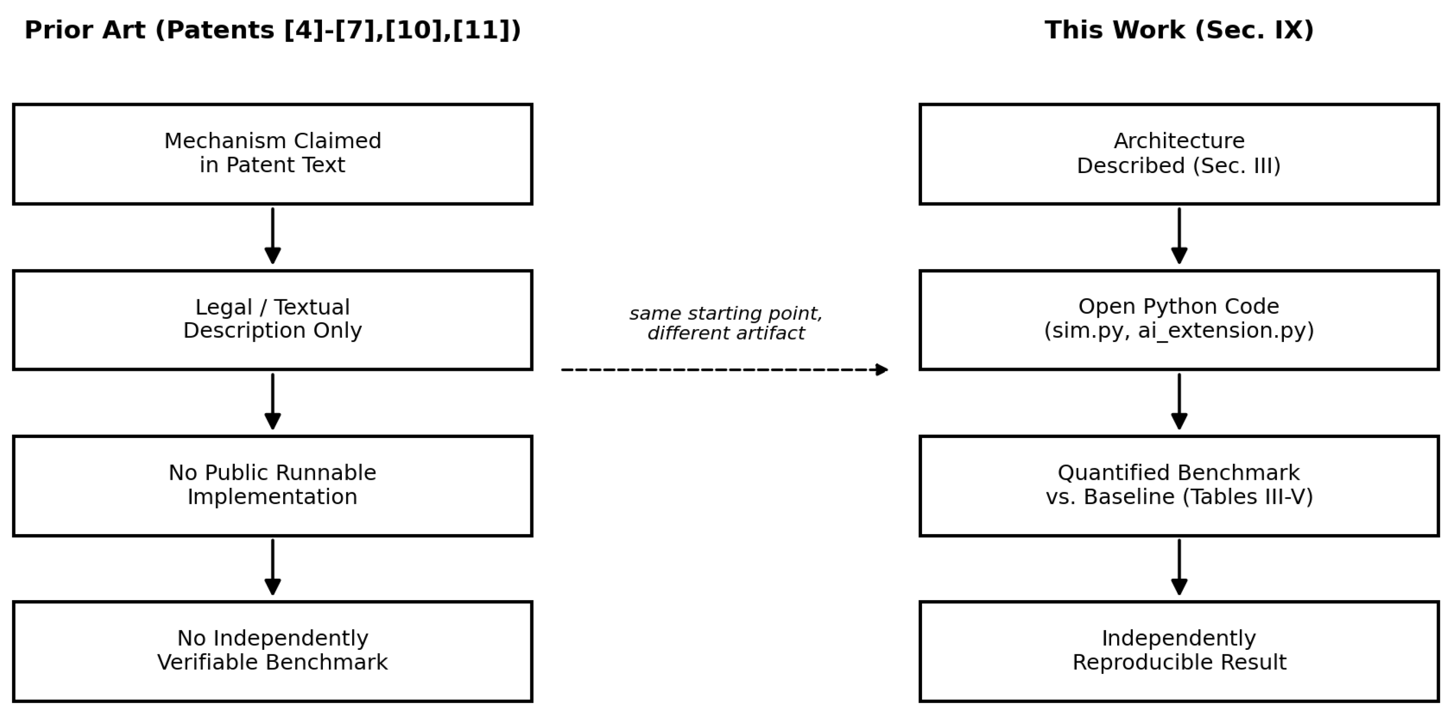
Every patent surveyed in Section II [4,5,6,7,10,11] is a legal and textual description of a mechanism: none is accompanied by a public, runnable implementation, a quantified benchmark against a baseline, or a dataset against which a third party can reproduce the claimed benefit. The production systems [8,9] are proprietary and closed. This is a structural limitation of patent documents and production automotive software generally, not a criticism specific to any one filing. Figure 12 contrasts the two artifacts side by side.
The contribution of this paper’s accompanying codebase (sim.py, ai_extension.py, run_experiment.py, run_ai_experiment.py) is therefore distinct from, and complementary to, the architectural novelty discussion of Sections II and X:
1) Reproducibility — every number reported in Tables III–V is regenerated by running the accompanying scripts; there is no hand-tuned or cherry-picked result that cannot be independently re-derived.
2) Quantitative baselines — the prior art establishes that predictive suspension control works in general; this implementation quantifies, on a controlled synthetic benchmark, how much a preview feedforward term specifically improves over a reactive-only skyhook controller (Section VII-D), and how much a learned fusion or gain-scheduling layer improves over the classical version of the same block (Section VIII) — comparisons not found reported in the patents themselves.
3) A negative-result record — Sections VII-D and VIII-C each report a design choice that initially made performance worse (an unfiltered feedforward derivative, and unsmoothed per-timestep gain switching) and the specific fix. Patent claims, by their nature, describe only the mechanism that is claimed to work; they do not document the failure modes encountered while arriving at it.
4) Extensibility — because the plant, fusion, and control layers are implemented as separate, independently testable Python modules, a third party can substitute a different plant model, sensor noise model, or controller (e.g., the model-predictive-control extension proposed in Section XI) without re-deriving the rest of the pipeline.
shows the specific function that implements novelty gap 1 of Section II-C — the seat actuator commanded from the same fused chassis-level estimate as the main suspension, rather than from an independent seat-local sensor set as in prior art [10]. This is the concrete code corresponding to (12)–(13).
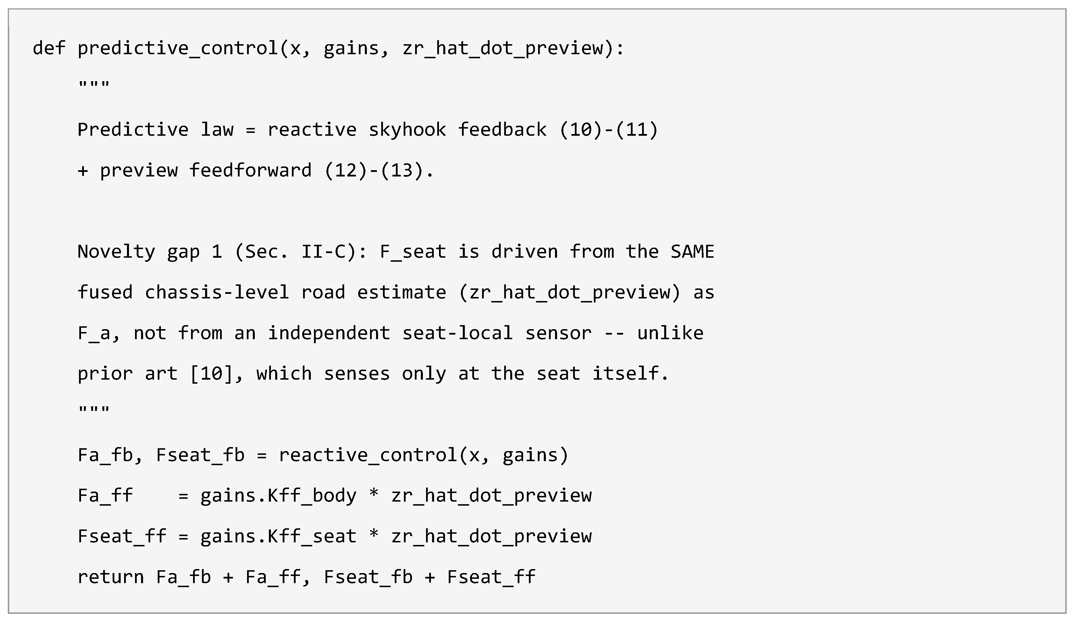
Listing 1. Seat-suspension actuator sharing the chassis-level fused road estimate (sim.py).
None of these four points is itself a patentable invention; reproducible code is not, by itself, a claimable method distinct from the method it implements. They are, however, a genuine contribution to the state of practice around this architecture, and are offered here as a complement to, not a substitute for, the freedom-to-operate discussion of Section X.
X. Limitations and Future Work
1) The plant model is a linearized-parameter quarter-car; a full vehicle model with roll/pitch coupling across four corners is needed before hardware claims can be made.
2) Sensor noise and dropout parameters (Section III-B2) are estimates from the literature reviewed, not measured from a specific production radar/camera stack; they should be re-fit once real logs (Table II, or the physical rig of Section VI) are available.
3) Model-predictive control with an explicit multi-step horizon, rather than the single-gain preview feedforward of (12)–(13), is a natural extension that would let the controller reason about the full sequence of upcoming bumps rather than one lookahead point.
4) Translating RMS acceleration reduction into a quantified injury/discomfort-risk reduction for elderly and pediatric occupants requires a biodynamic multi-segment occupant model per ISO 5982, not just the lumped seat mass used in (9).
XI. Conclusions
This paper formalized a sensor-fusion-driven predictive suspension and seat-suspension architecture, situated it precisely against a documented body of prior art, and evaluated it quantitatively in a reproducible Python simulation. The predictive controller improved ISO 2631-weighted comfort by 23.7% (chassis) and 67.9% (seat) over a passive baseline; learned sensor fusion improved road-preview accuracy by 27.2% over the classical fusion law on unseen terrain; and terrain-adaptive gain scheduling produced a smaller, honestly reported 0.8–3.5% further improvement, limited chiefly by classifier accuracy. The architecture itself is not patentably novel, but three narrow implementation choices — chassis-fused seat actuation, off-road terrain targeting, and graceful sensor-dropout degradation — remain candidate claims pending formal legal review, and the accompanying open, runnable implementation is offered as a contribution distinct from, and complementary to, that legal question.
XII. IEEE Dataport: Dataset and Code Availability
The complete simulation dataset (time-series CSVs for the road profile, multi-sensor previews, fused road estimate, and all three controller responses), the Python code that generated it, every figure in this paper, and this manuscript are permanently archived on IEEE DataPort under a CC BY 4.0 license:
AI-Enhanced Predictive Suspension Control — IEEE DataPort (https://ieee-dataport.org/documents/ai-enhanced-predictive-suspension-control-sensor-fusion-machine-learning-and-terrain)
A. Repository Contents
The DataPort repository is organized into four top-level folders. data/ contains seven CSV files: road_profile.csv, sensor_previews.csv, fused_estimate.csv, and controller_responses.csv (the raw 500 Hz time-series underlying Figs. 3–6 and Table III), plus three summary tables reproducing Tables III–V. code/ contains sim.py, ai_extension.py, run_experiment.py, run_ai_experiment.py, make_diagrams.py, and requirements.txt — the same code reproduced in full in the Appendix A. figures/ contains all twelve paper figures plus a graphical abstract. docs/ contains this manuscript and a column-level data dictionary (DATASET_DOCUMENTATION.md).
B. Reproducing the Results
Every number in Tables III–V and every figure in this paper can be regenerated from the repository with:
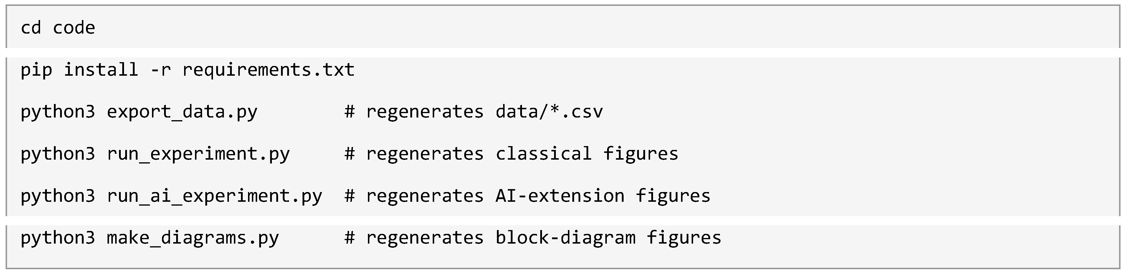
Reproduction commands (also listed in the repository README).
C. Citation Requirements
Researchers who use this dataset or code are requested to cite both the dataset and this article. Full citation templates, including DOI fields, are provided in the repository’s DATASET_DOCUMENTATION.md and LICENSE.txt files.
Appendix A
This appendix reproduces, in full, the four Python modules whose methodology and outputs are described in Sections III, VII, and VIII: sim.py (core physics plant, sensor and fusion models, skyhook and predictive control laws), ai_extension.py (learned fusion and terrain classification, Section VIII), run_experiment.py (the classical-pipeline experiment driver reproducing Section VII), and run_ai_experiment.py (the AI-extension experiment driver reproducing Section VIII). All four files, together with requirements.txt and the diagram-generation scripts, are also available at the IEEE DataPort repository cited in Section XII.
Appendix A.1. sim.py
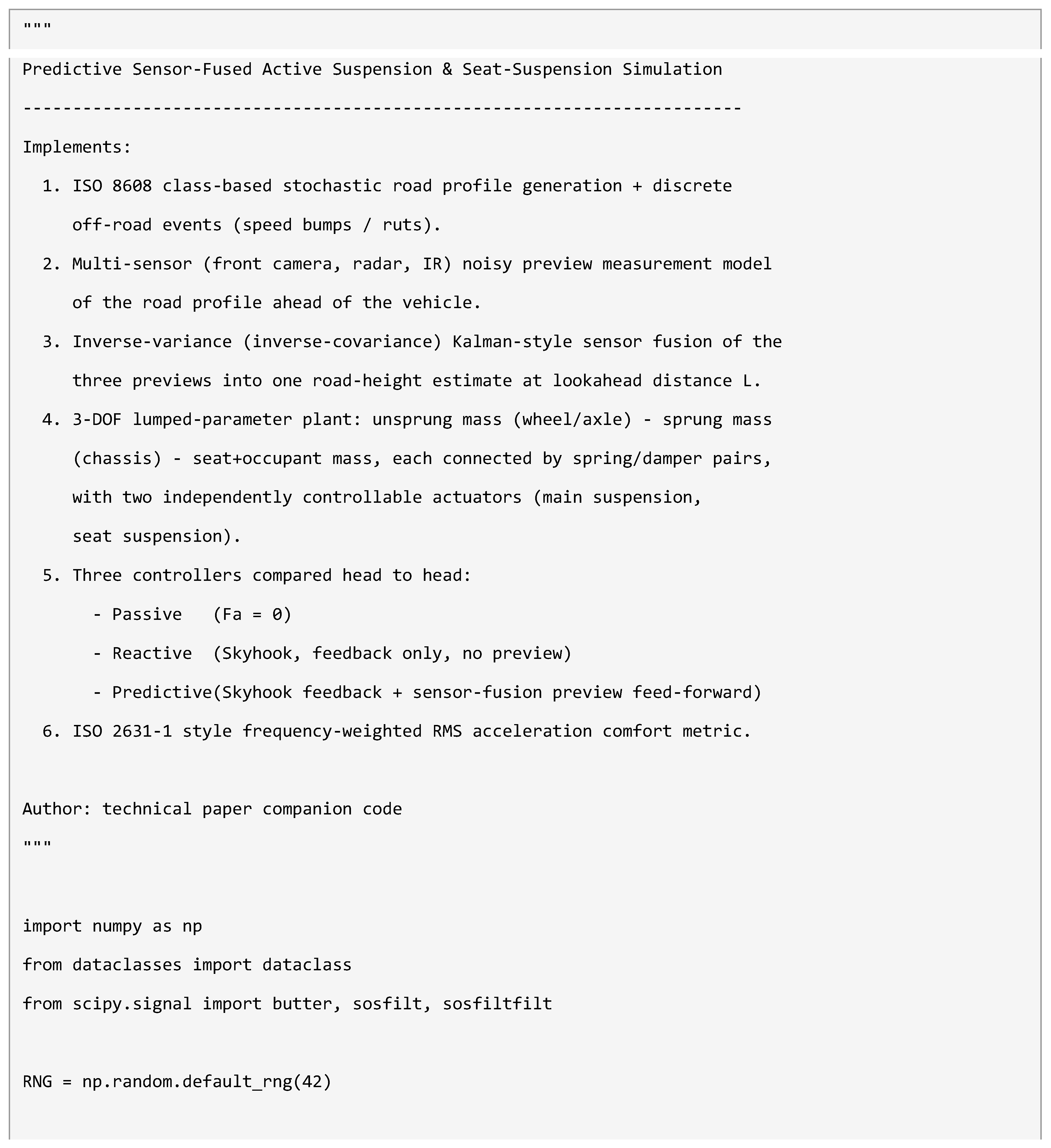
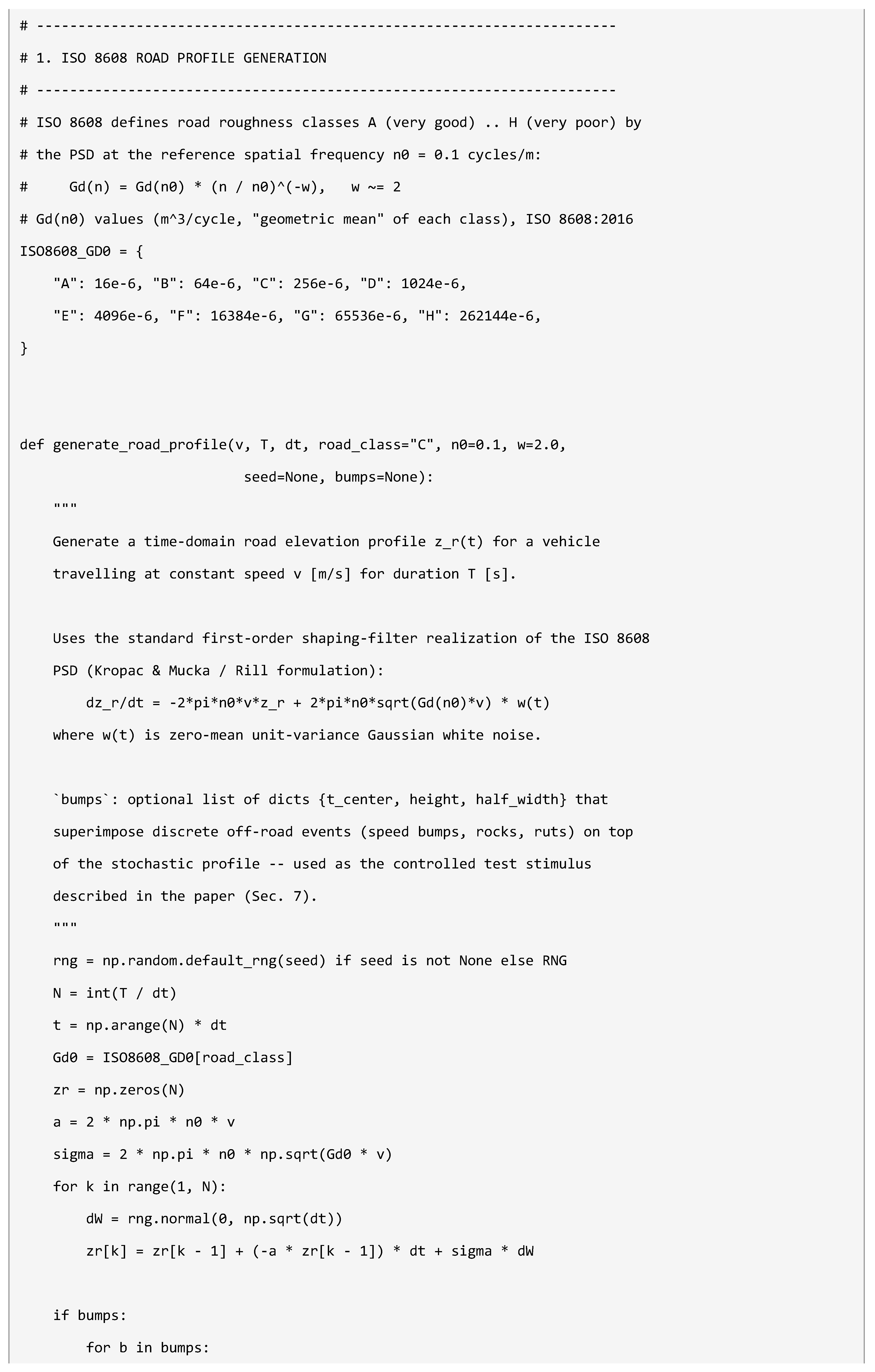
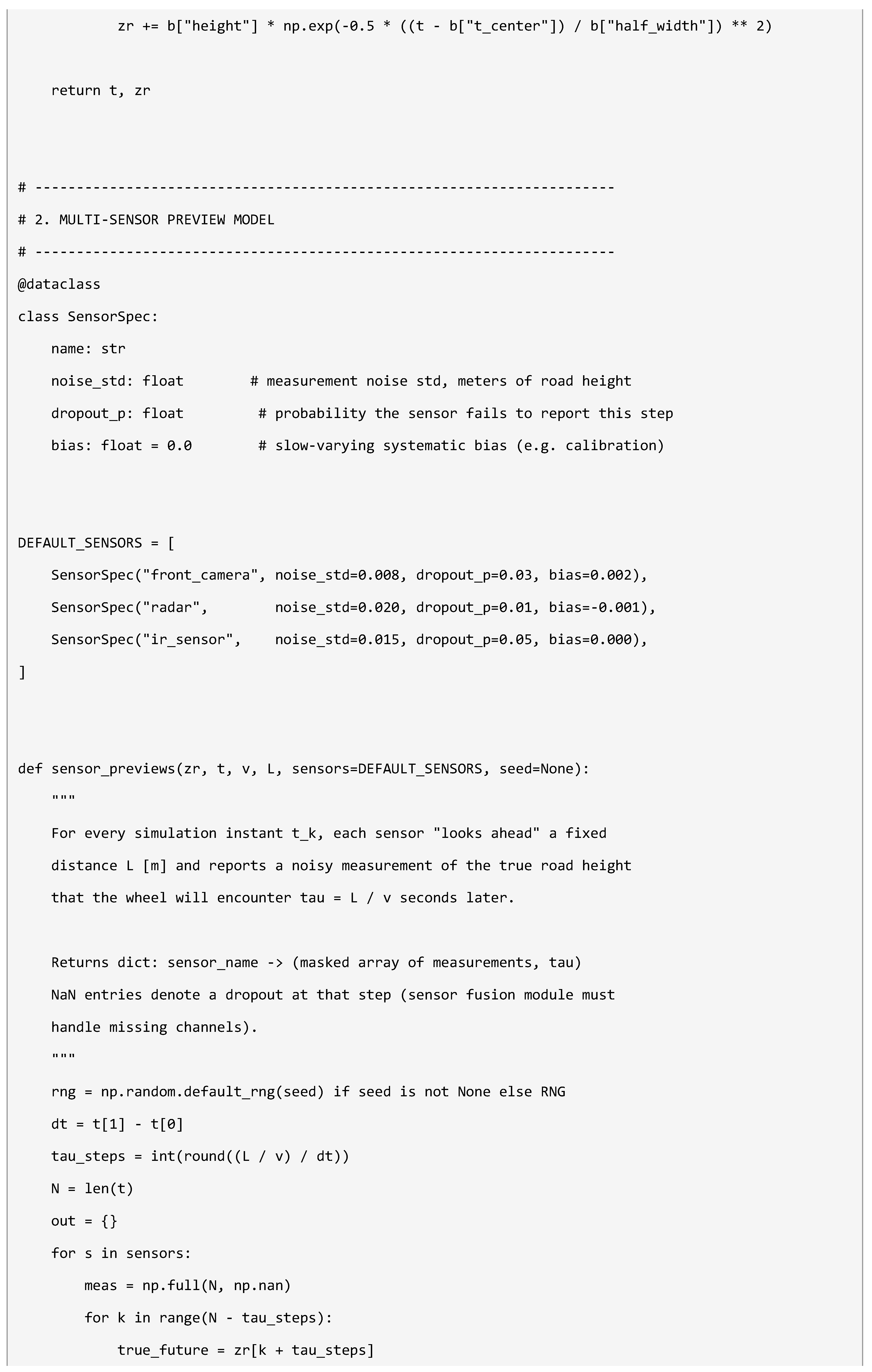
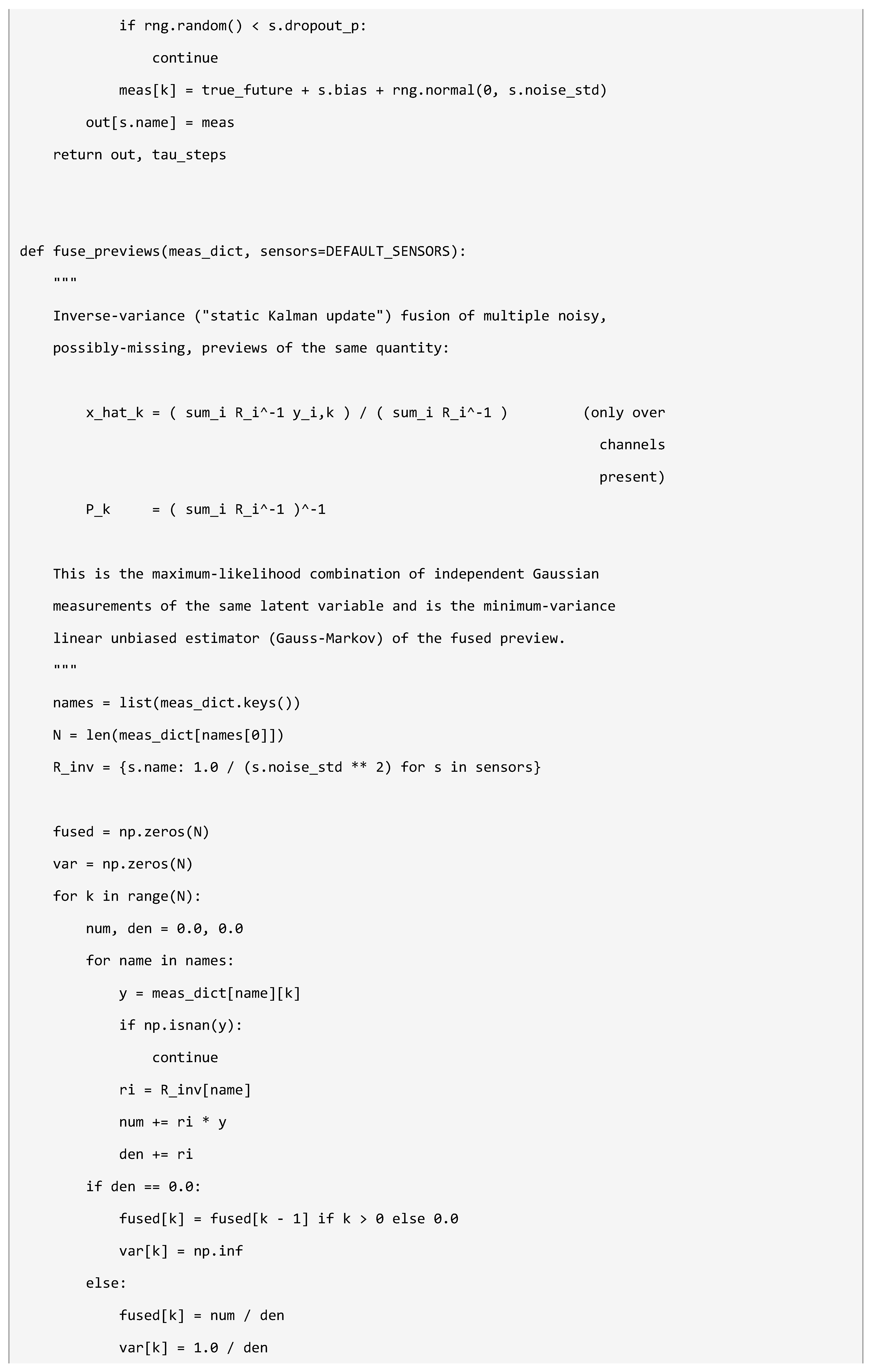
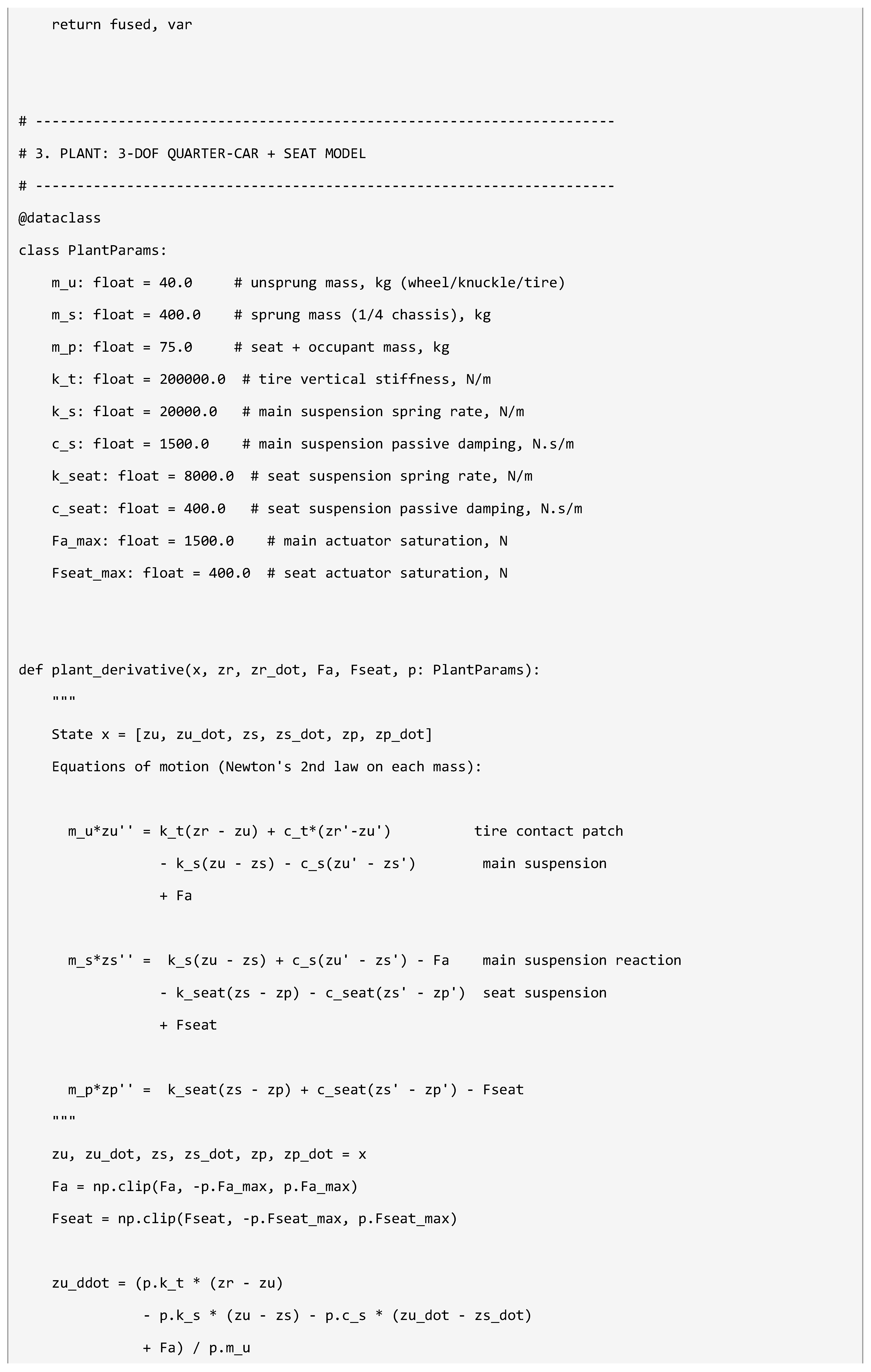
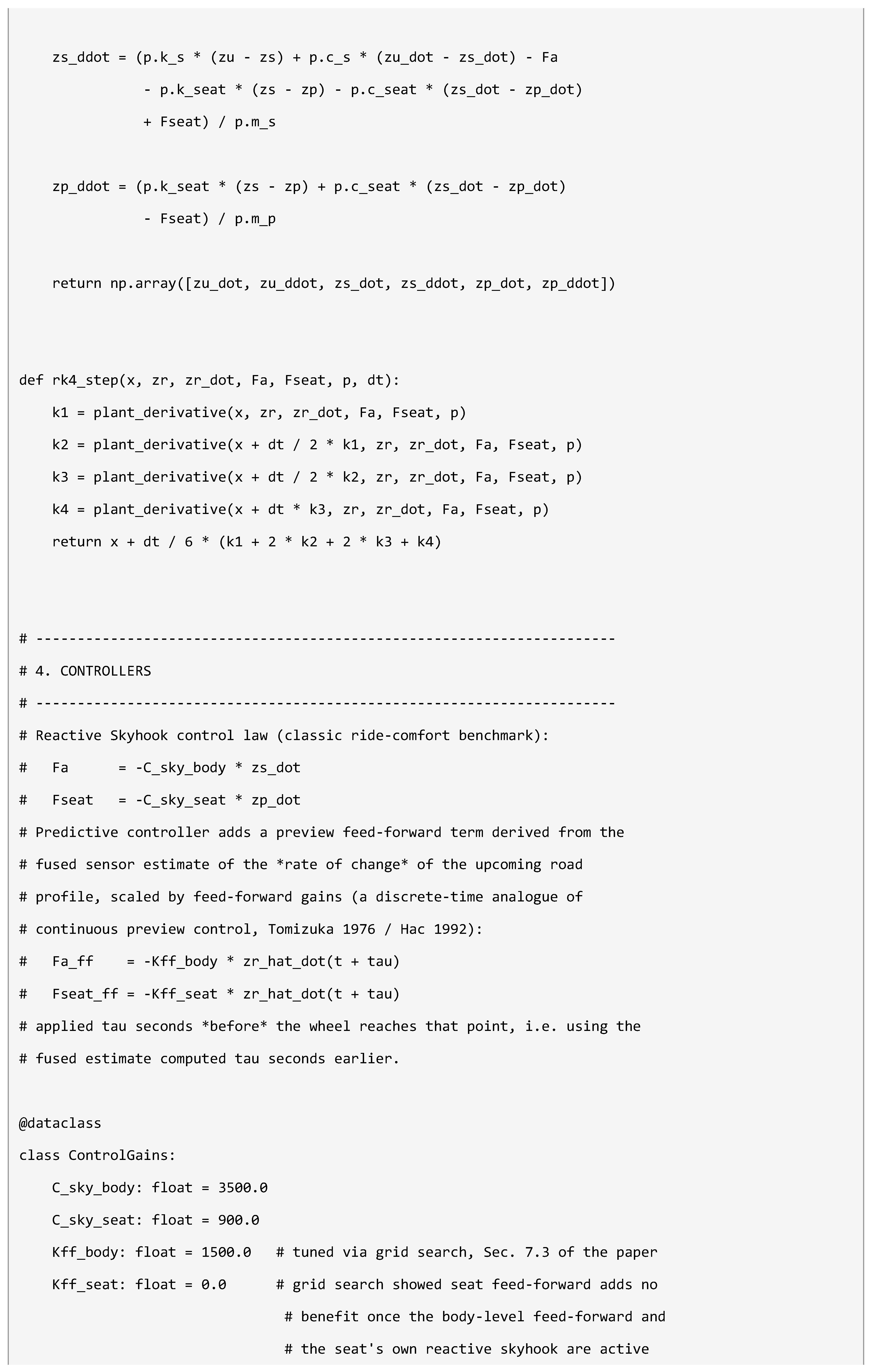
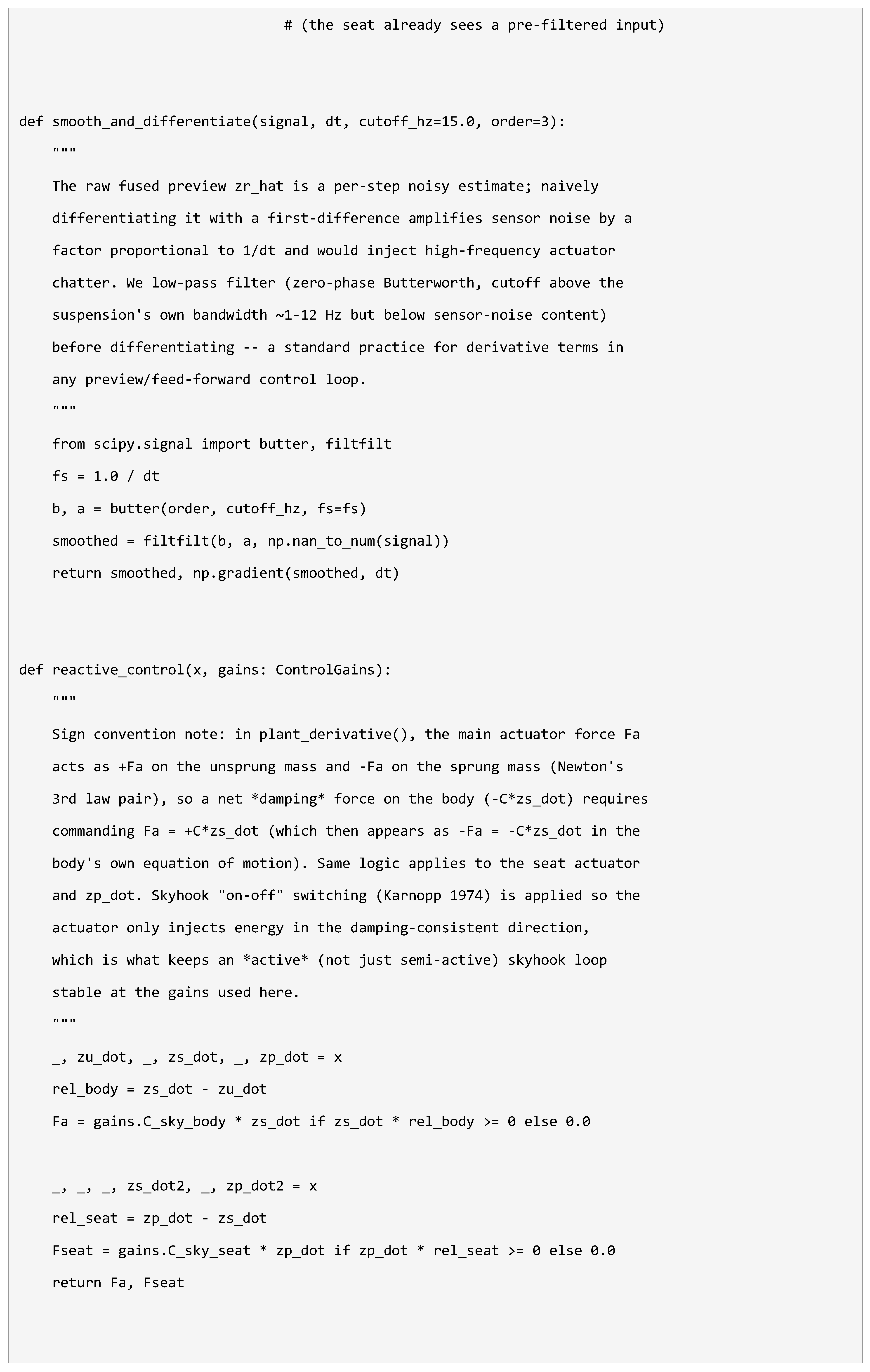
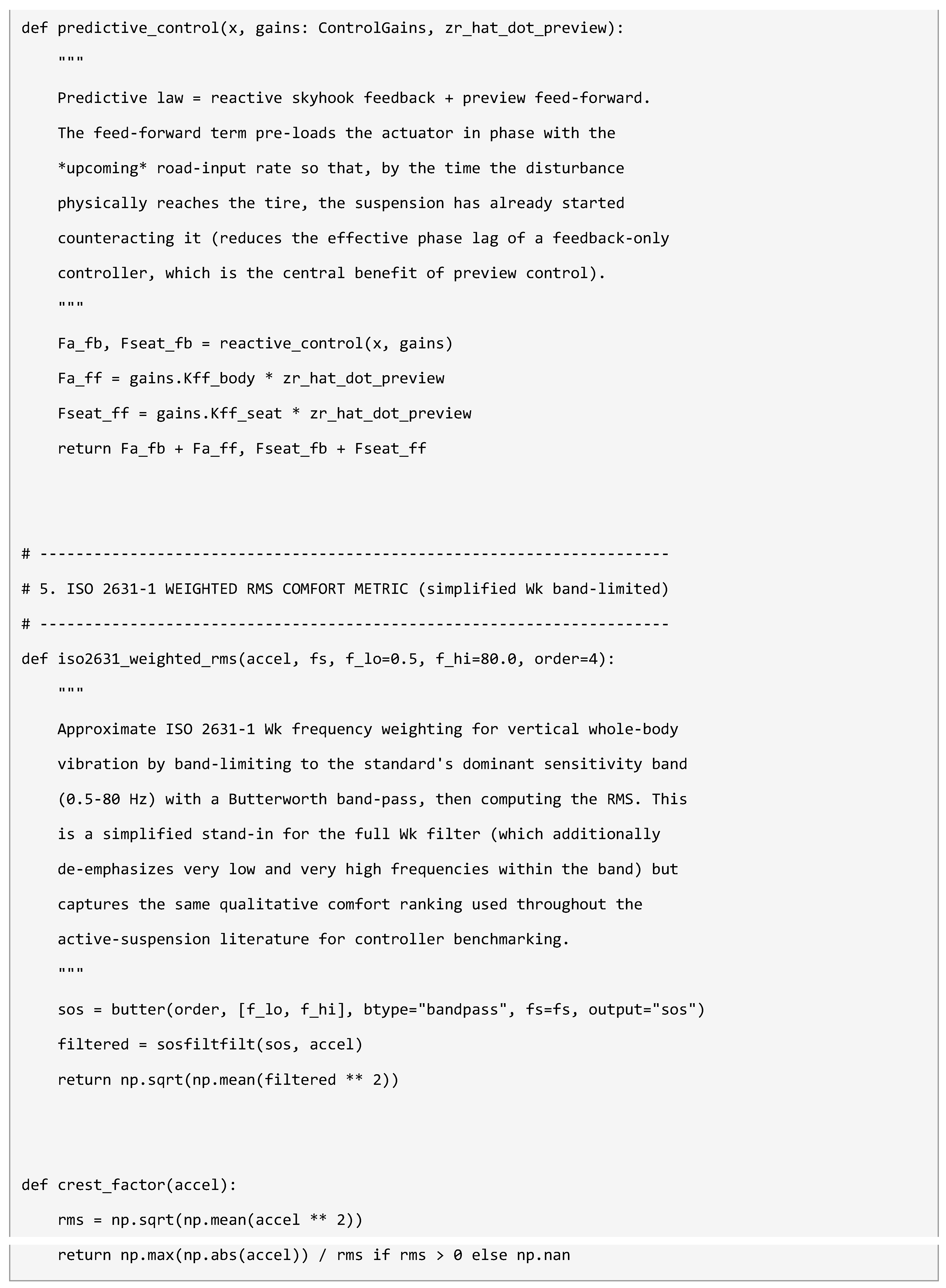
Listing A1. Full contents of sim.py.
Appendix B. ai_extension.py
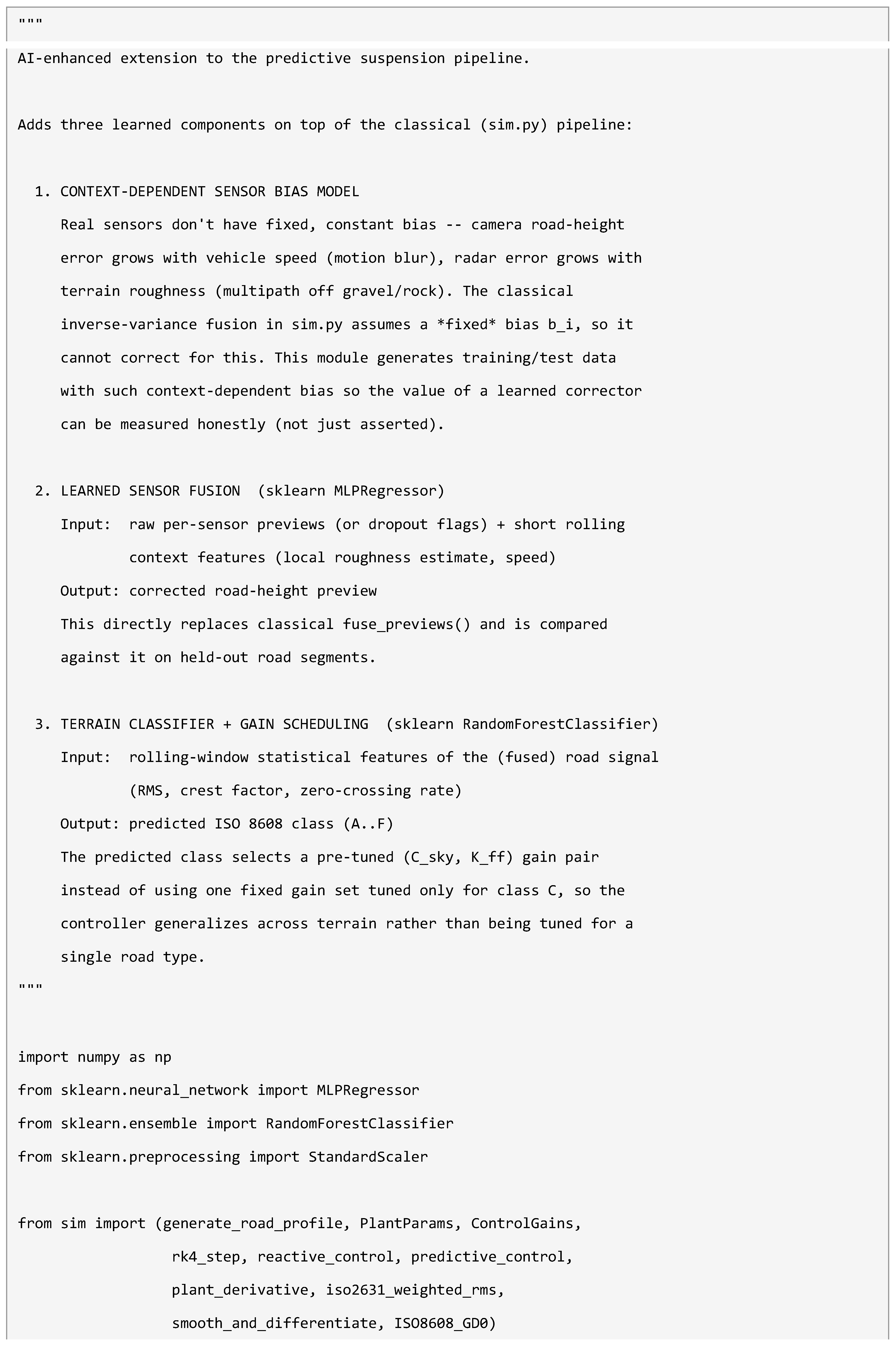
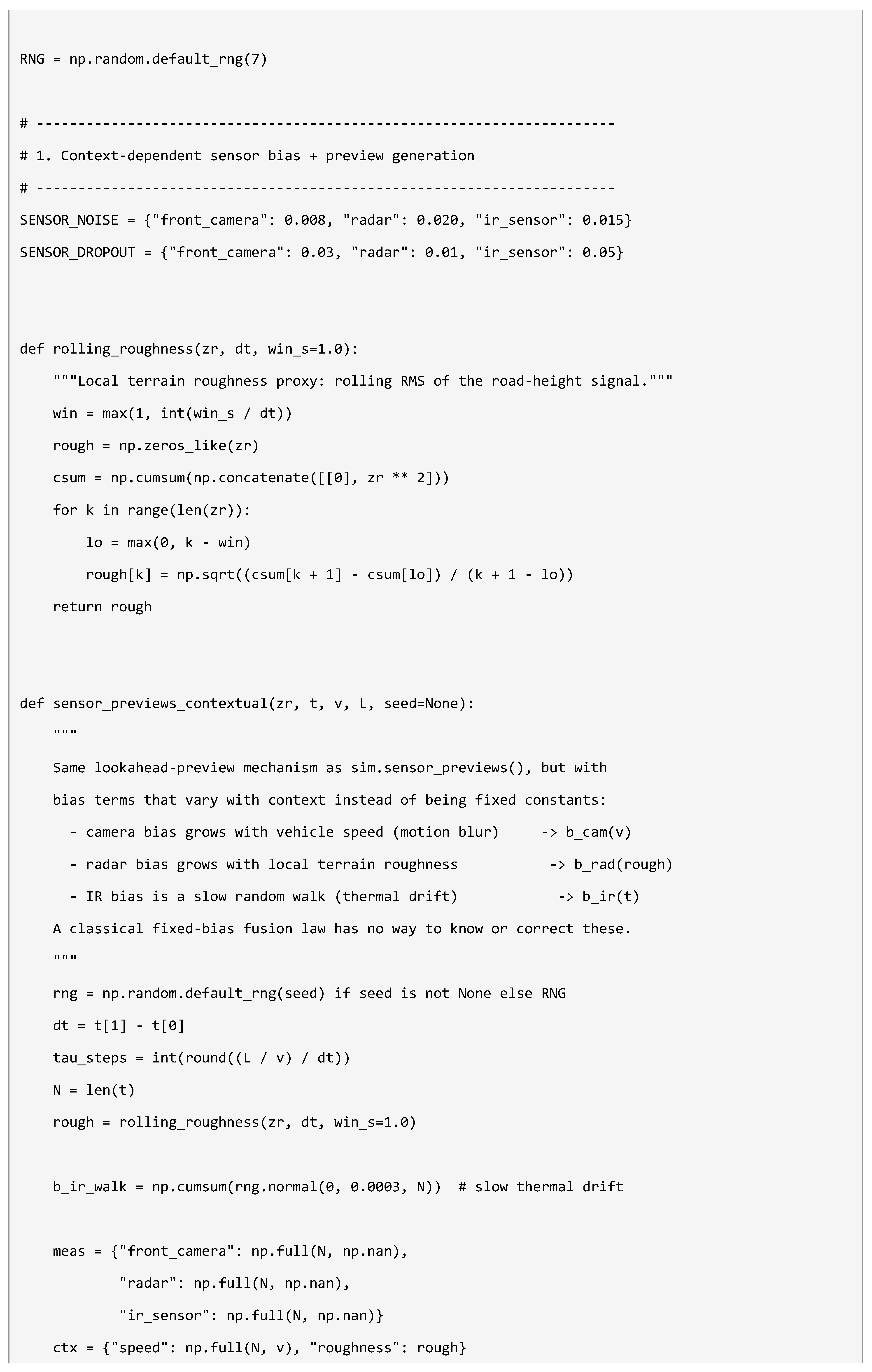
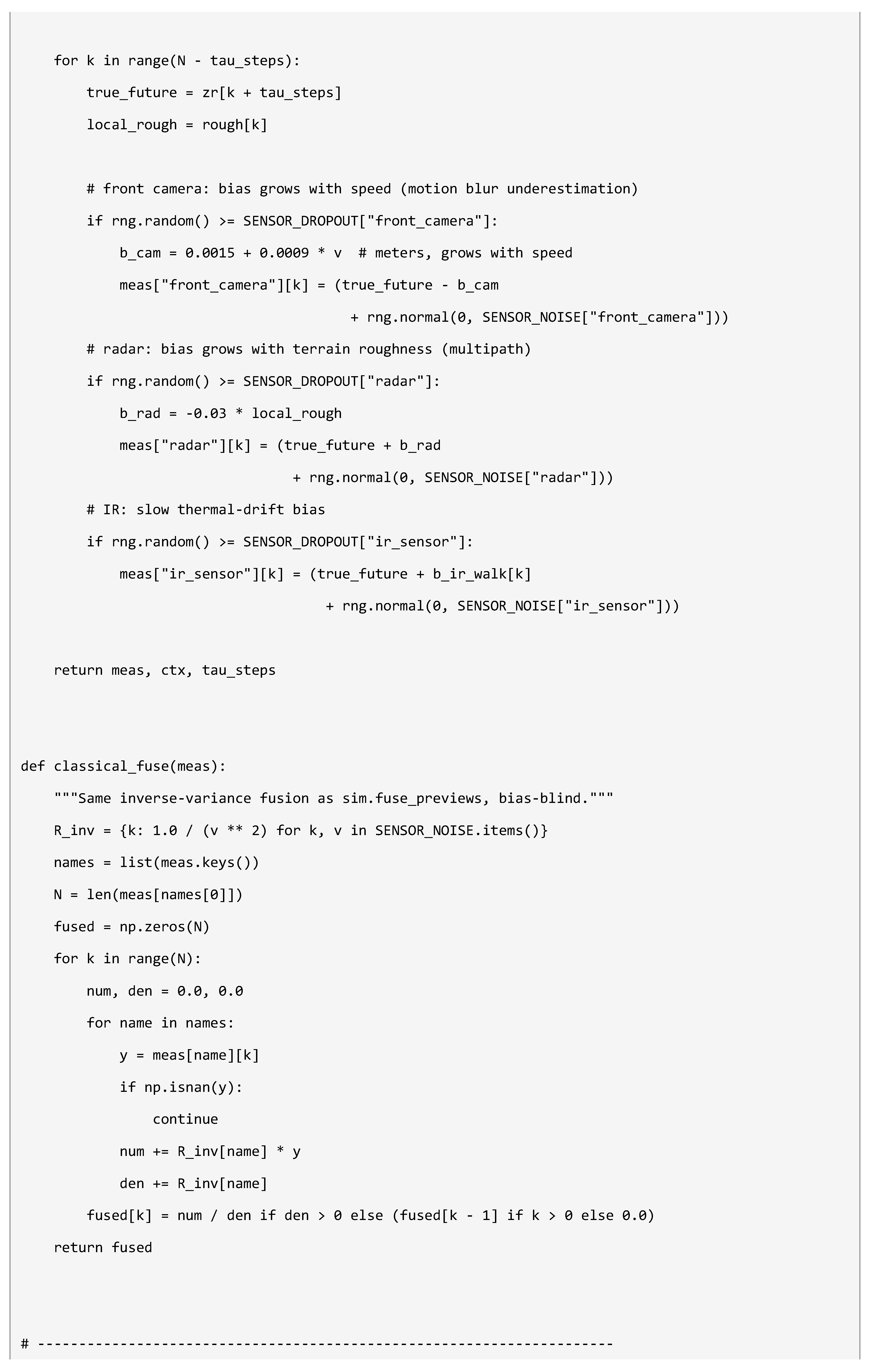
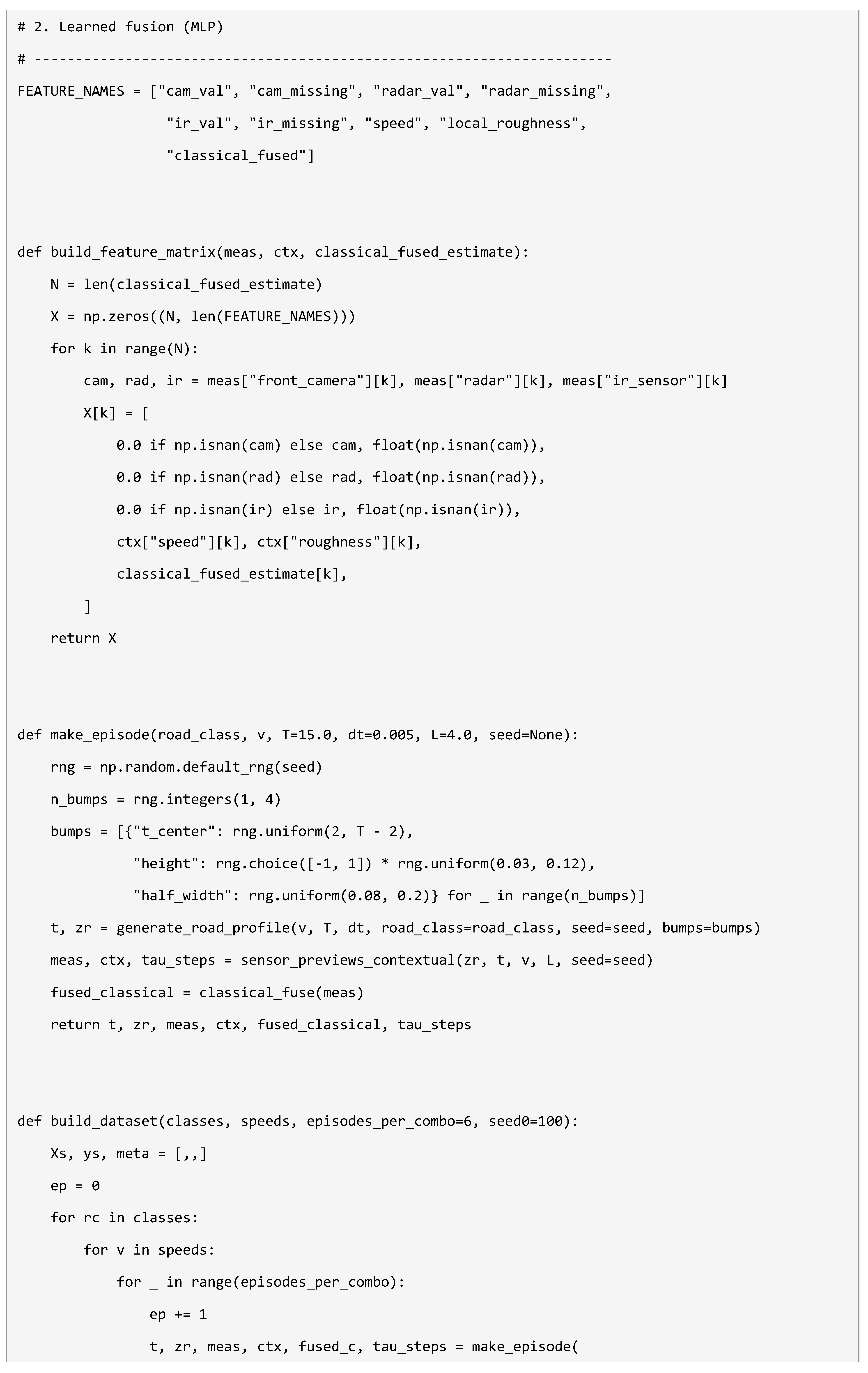
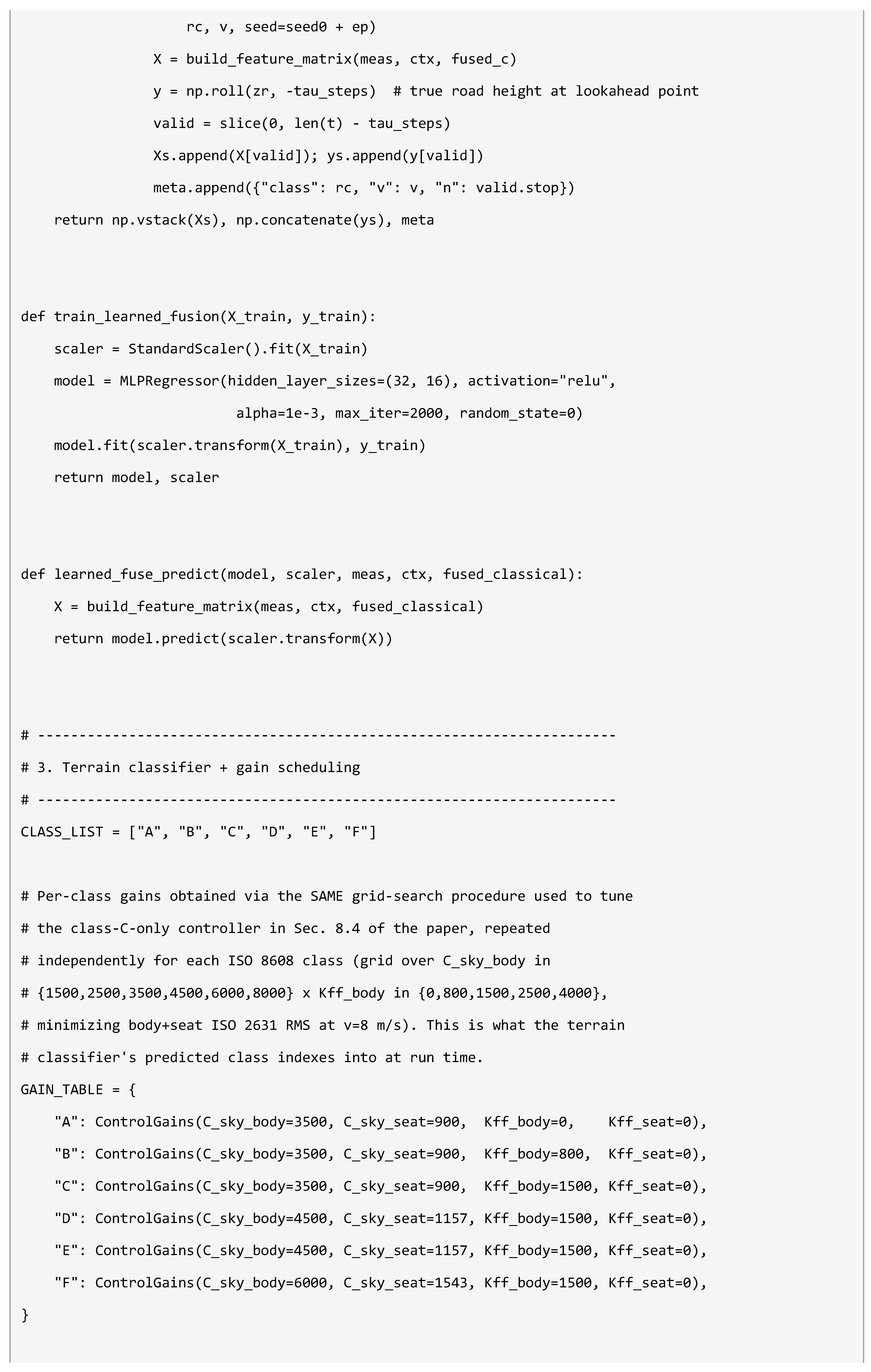
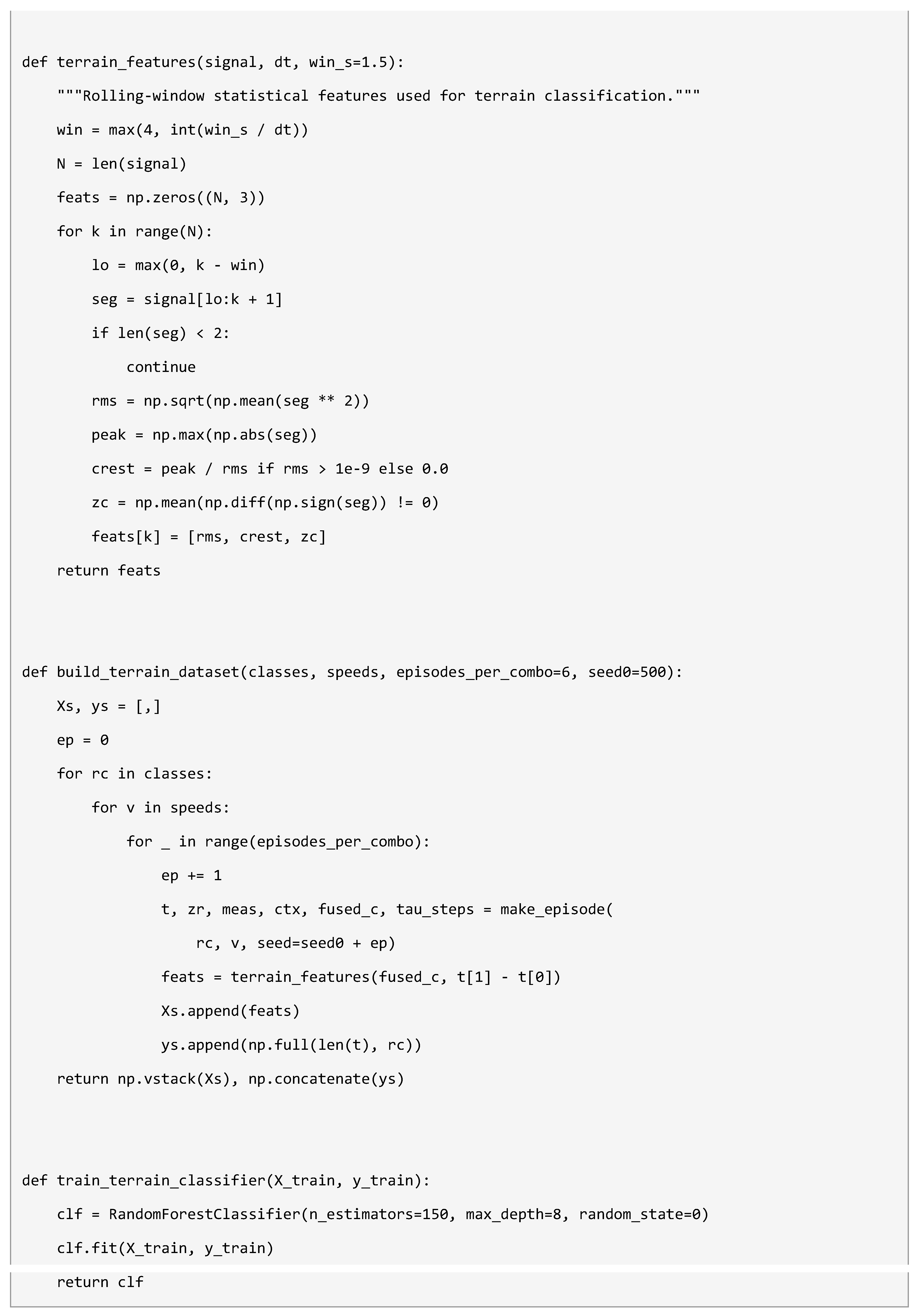
Listing A2. Full contents of ai_extension.py.
Appendix C. run_experiment.py
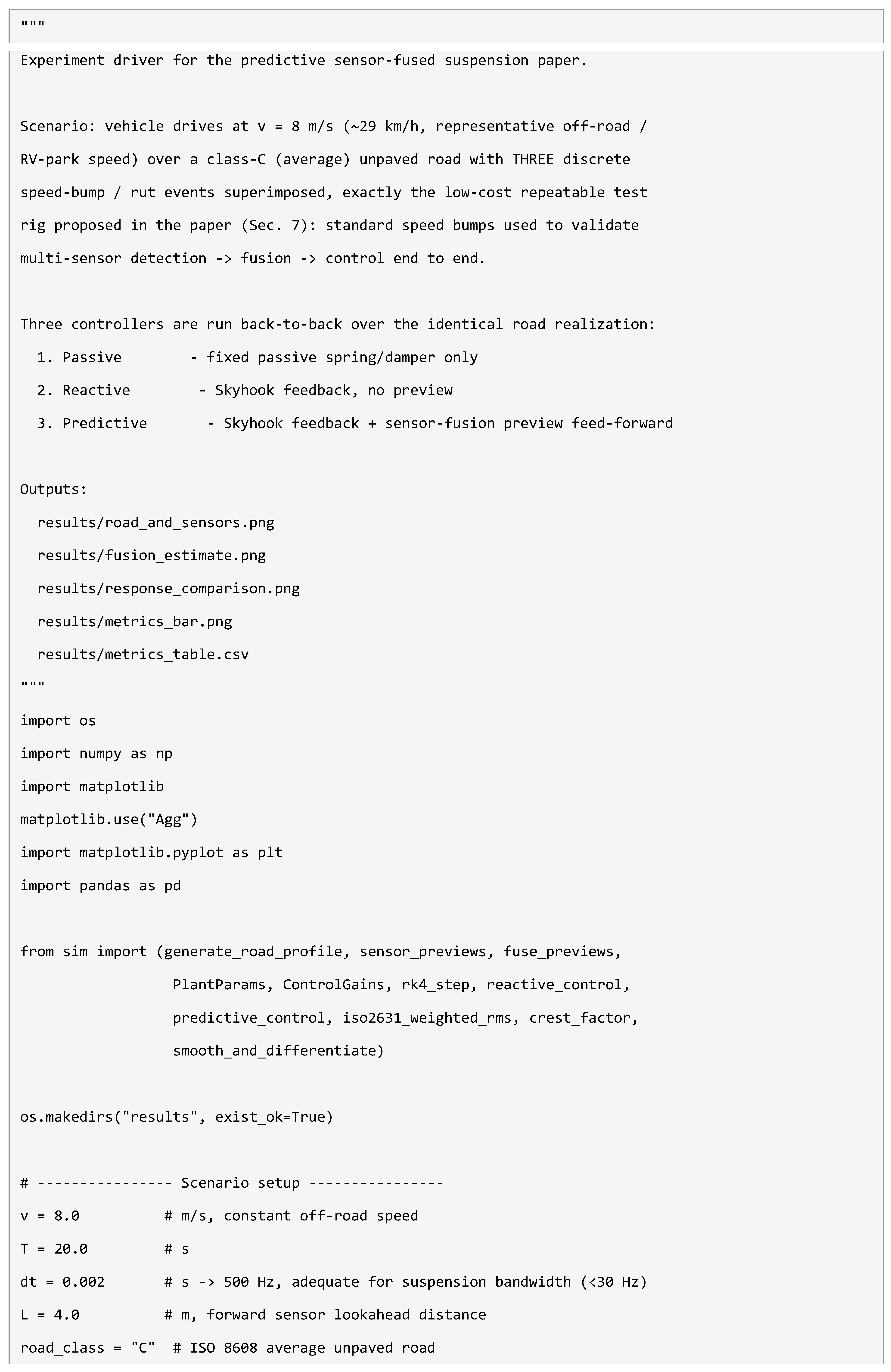
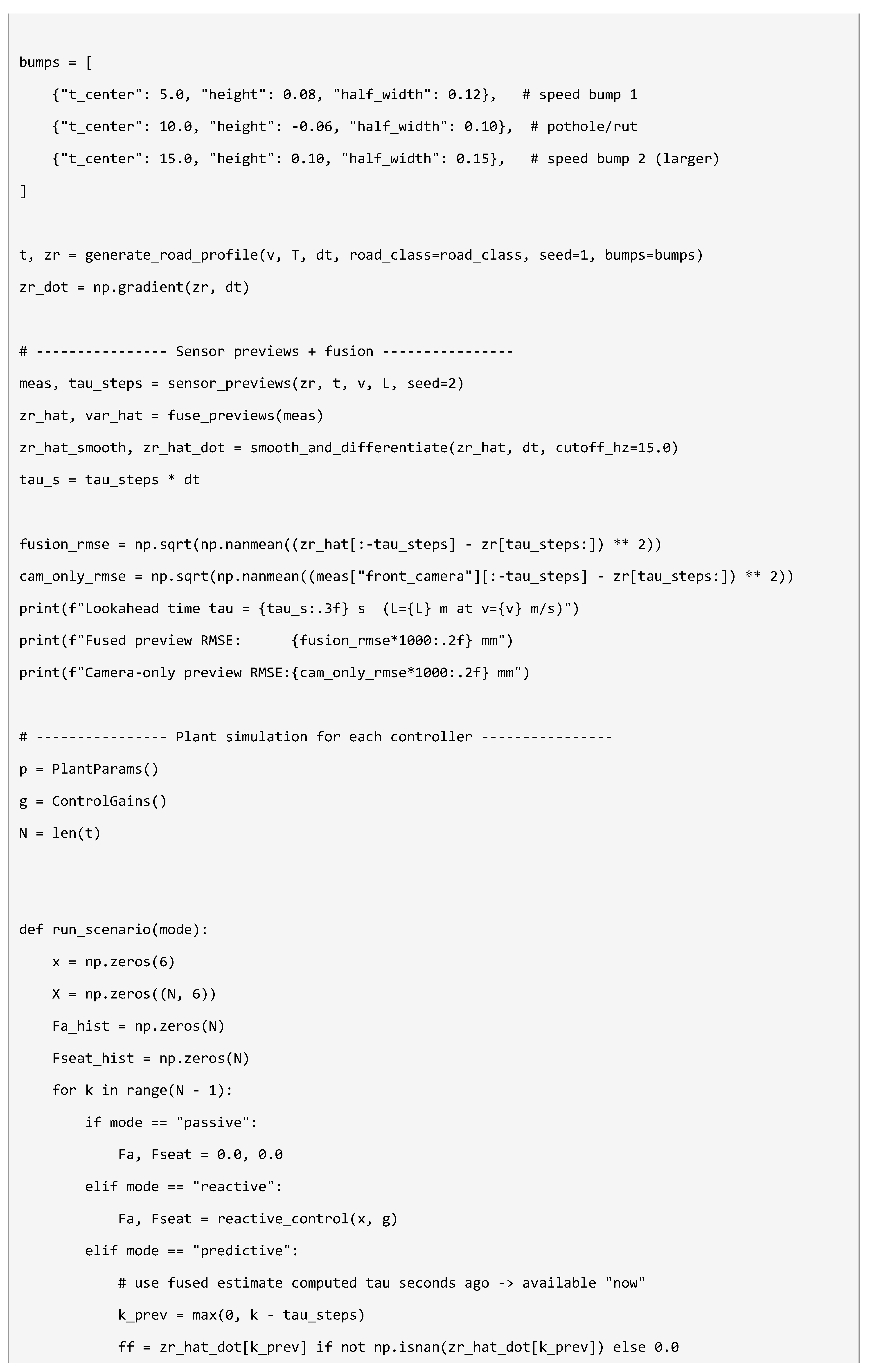
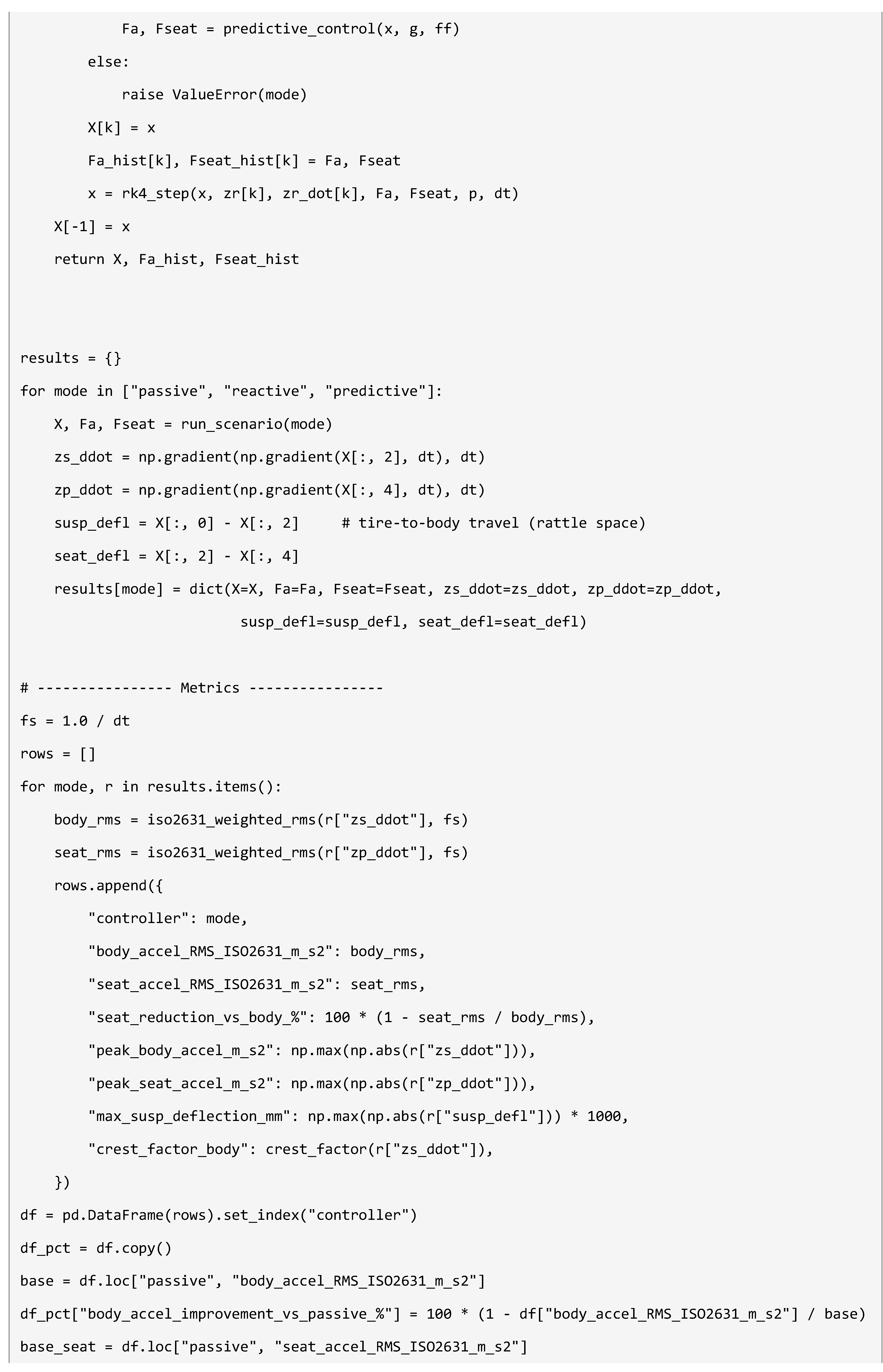
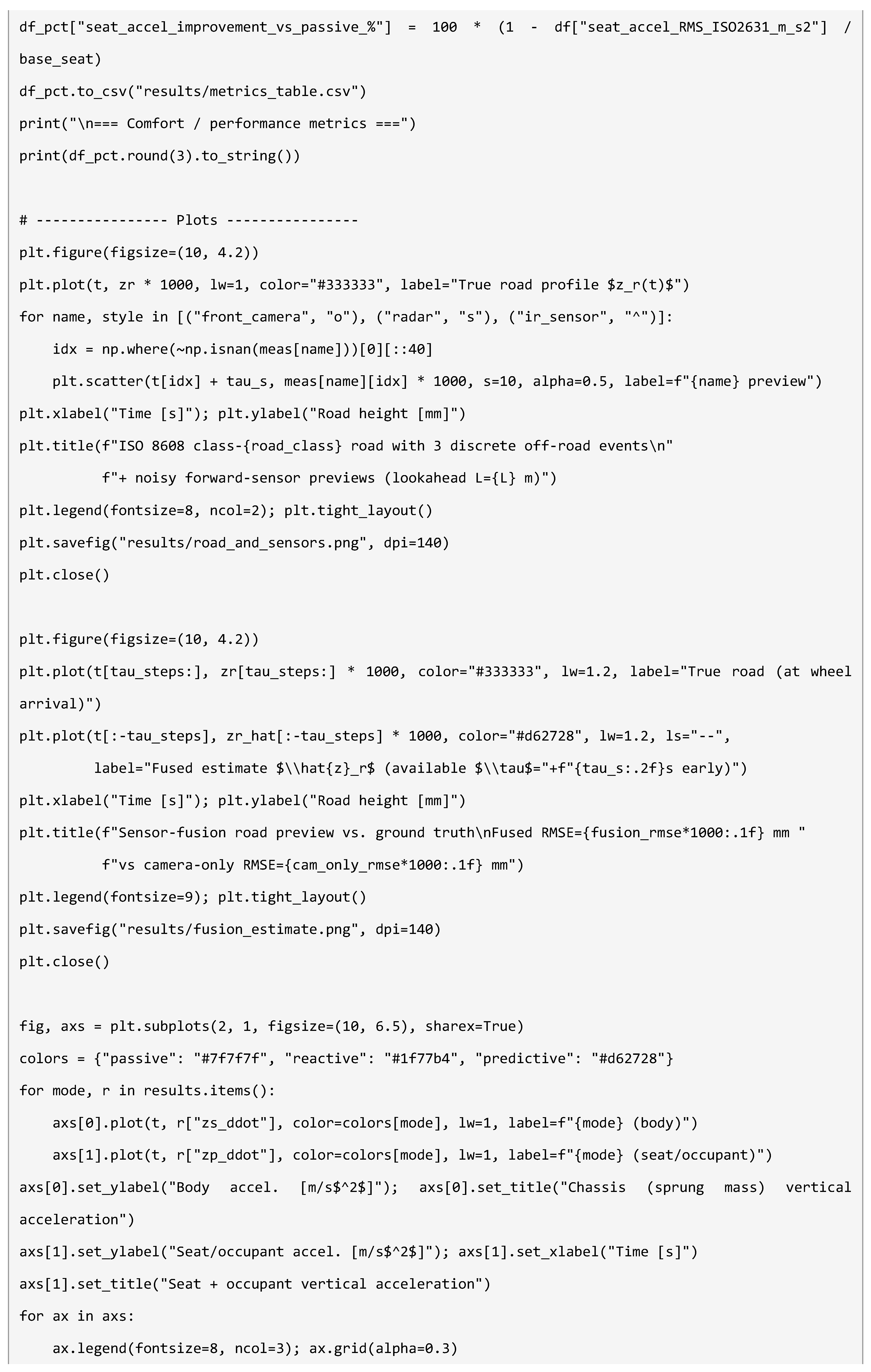
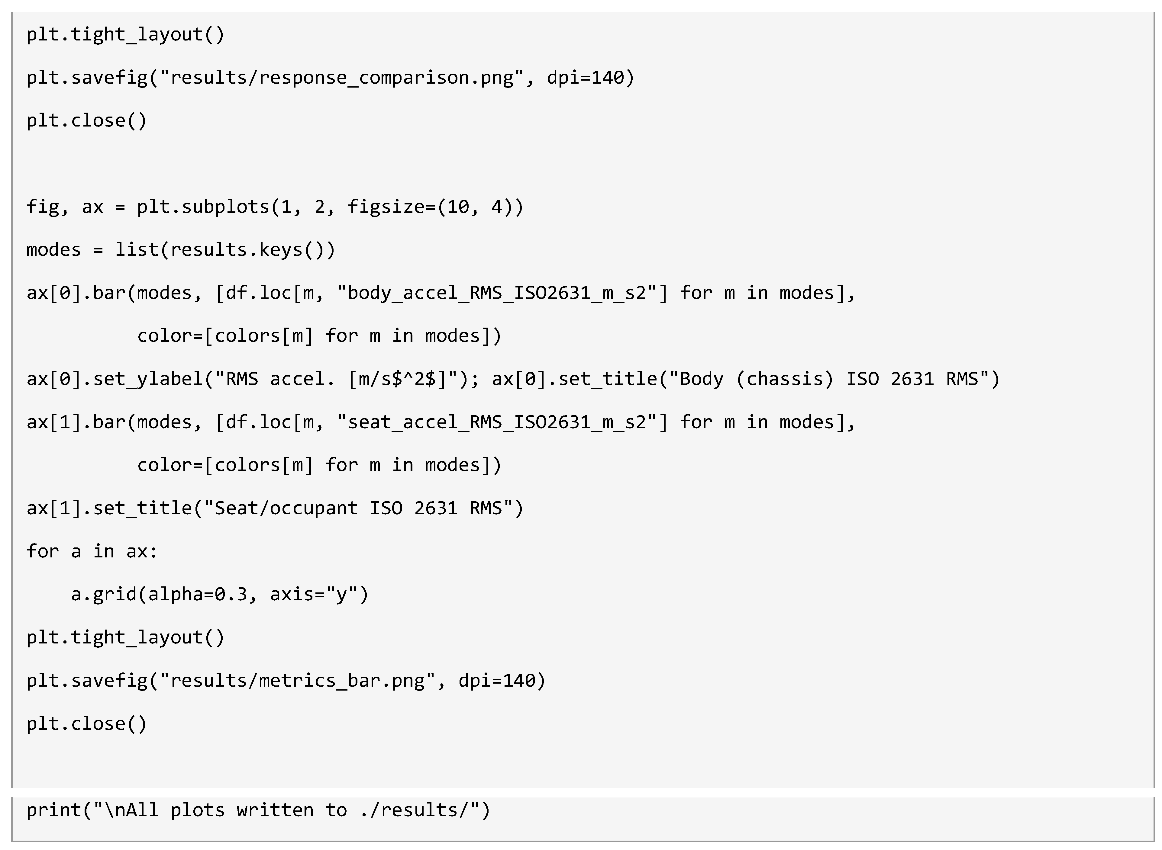
Listing A3. Full contents of run_experiment.py.
Appendix D. run_ai_experiment.py
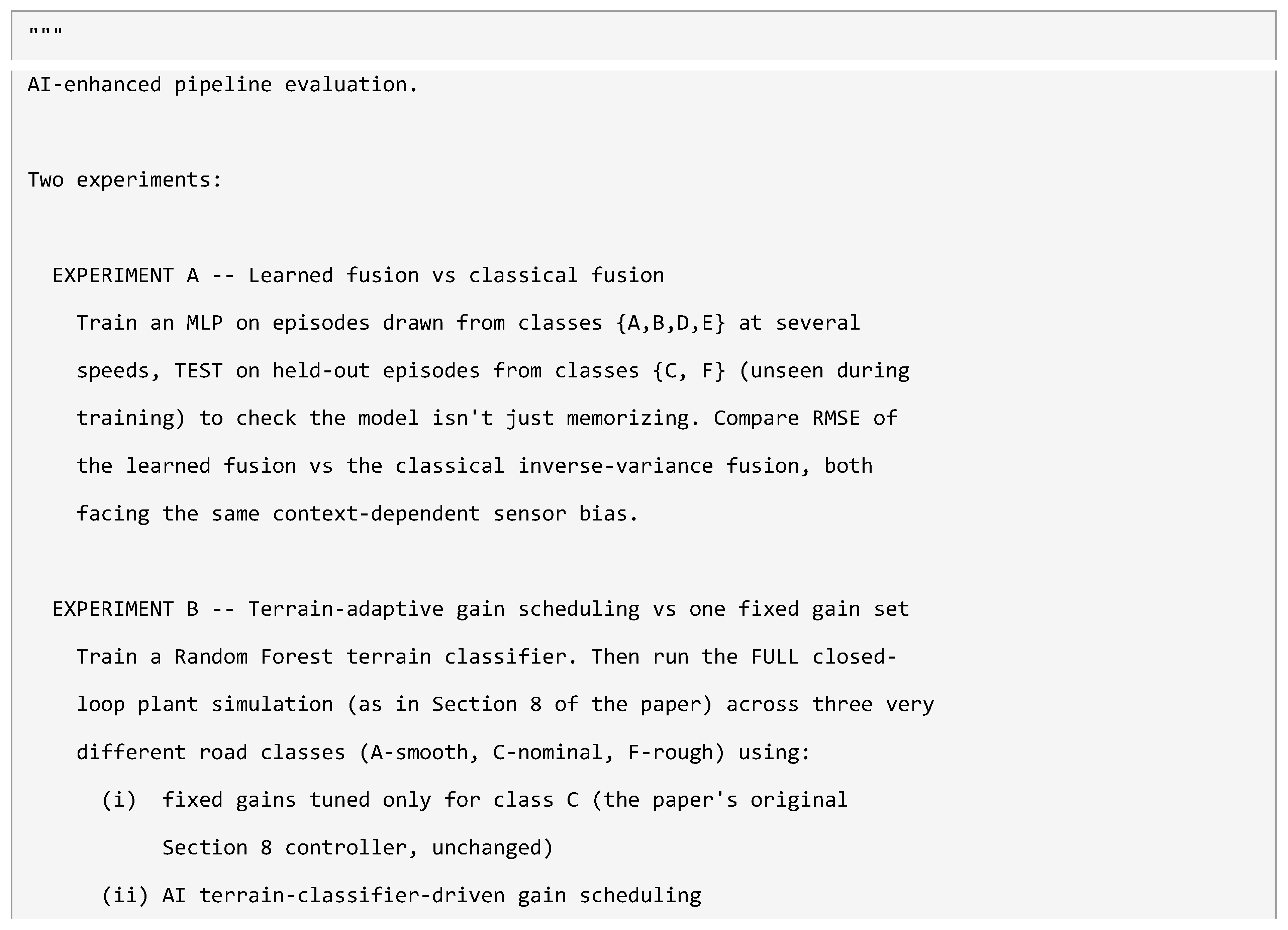
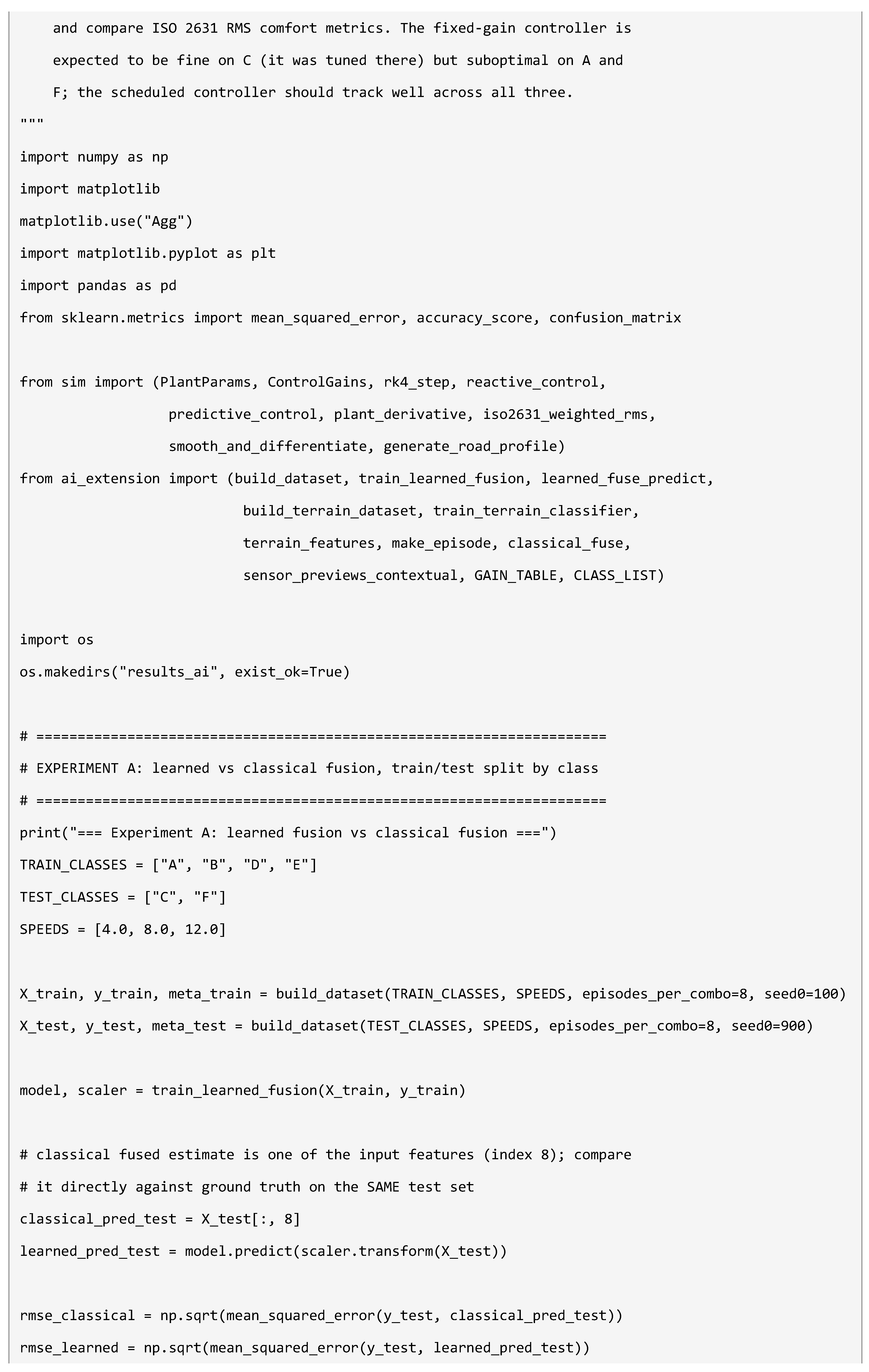
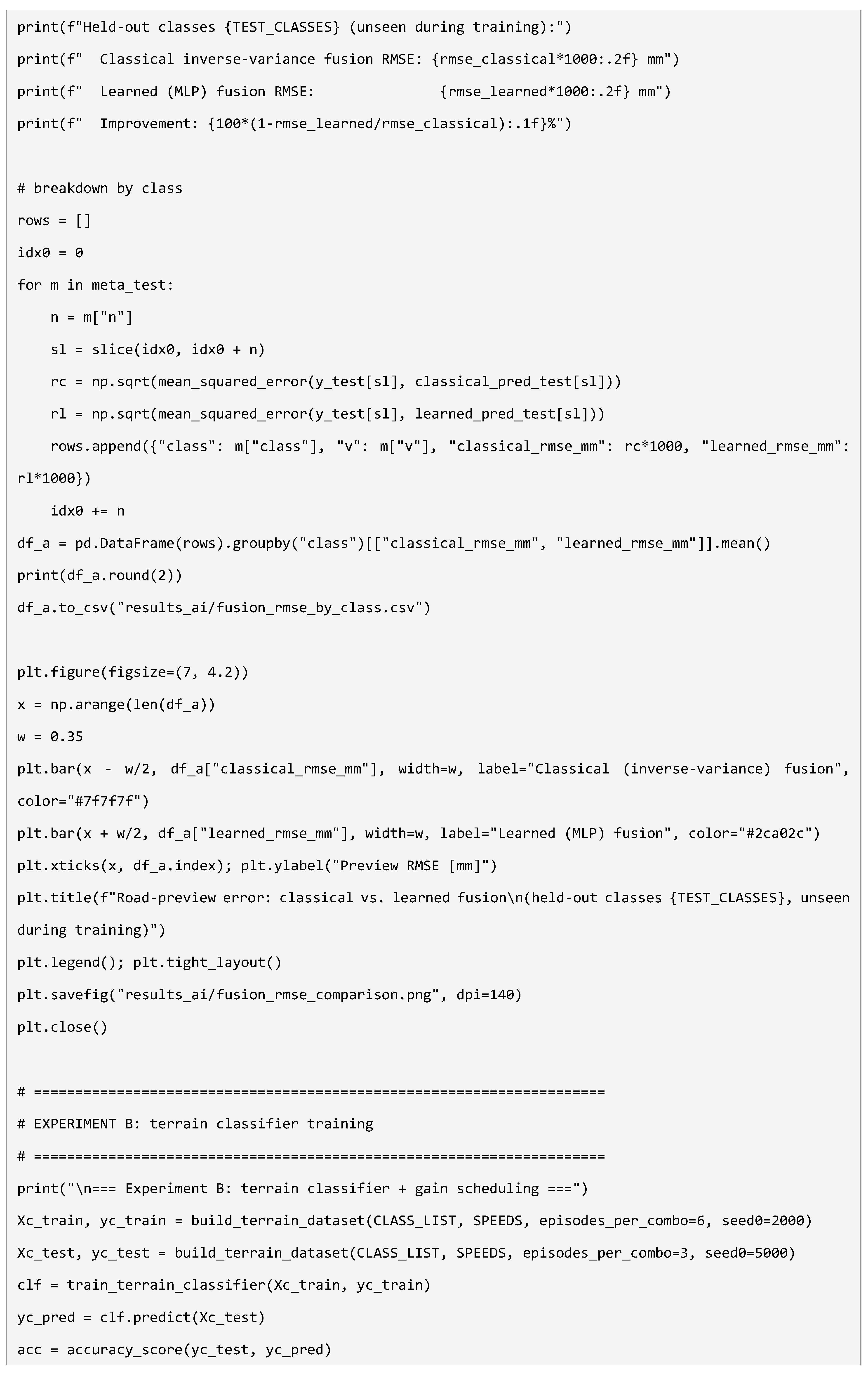
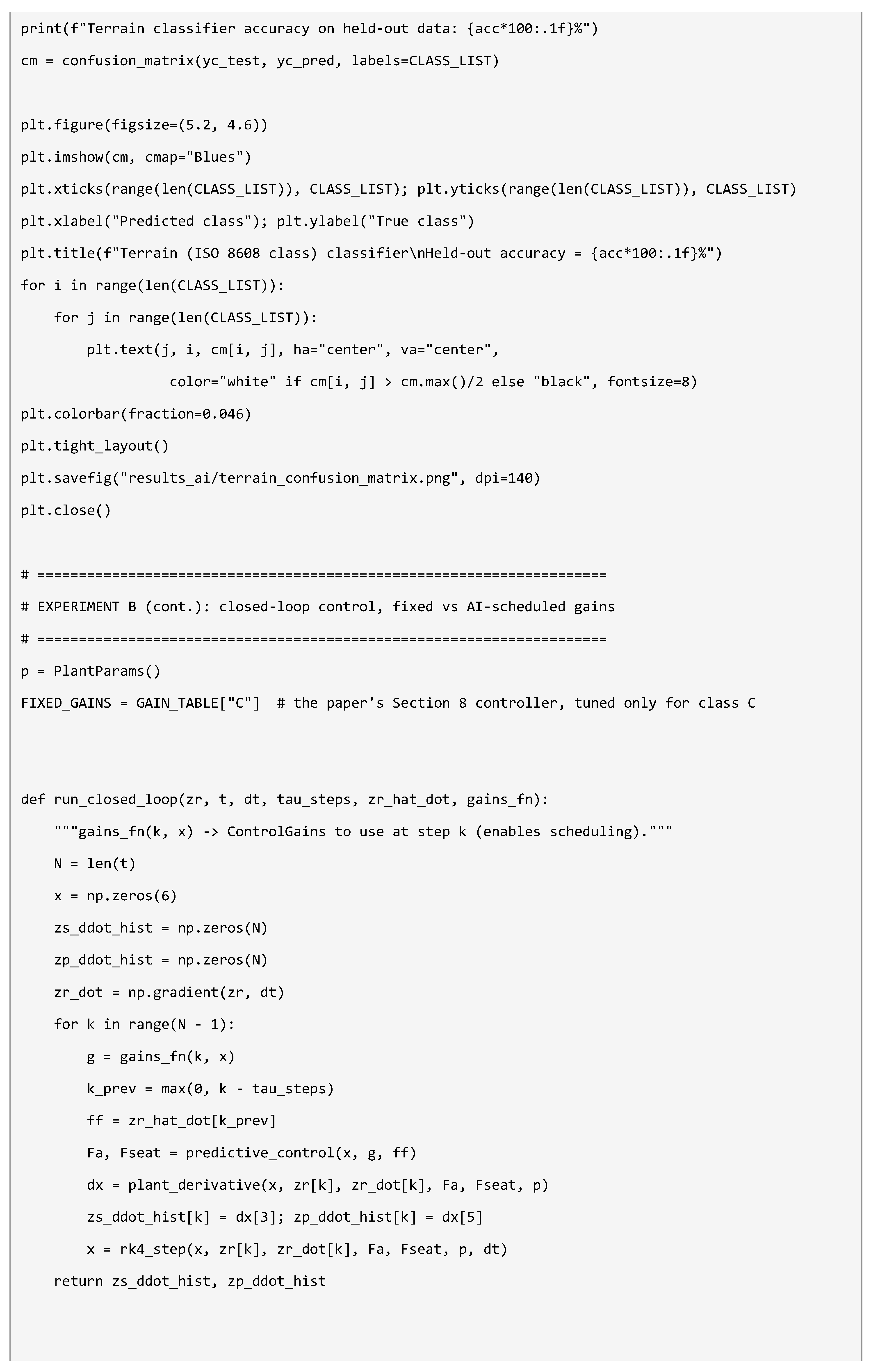
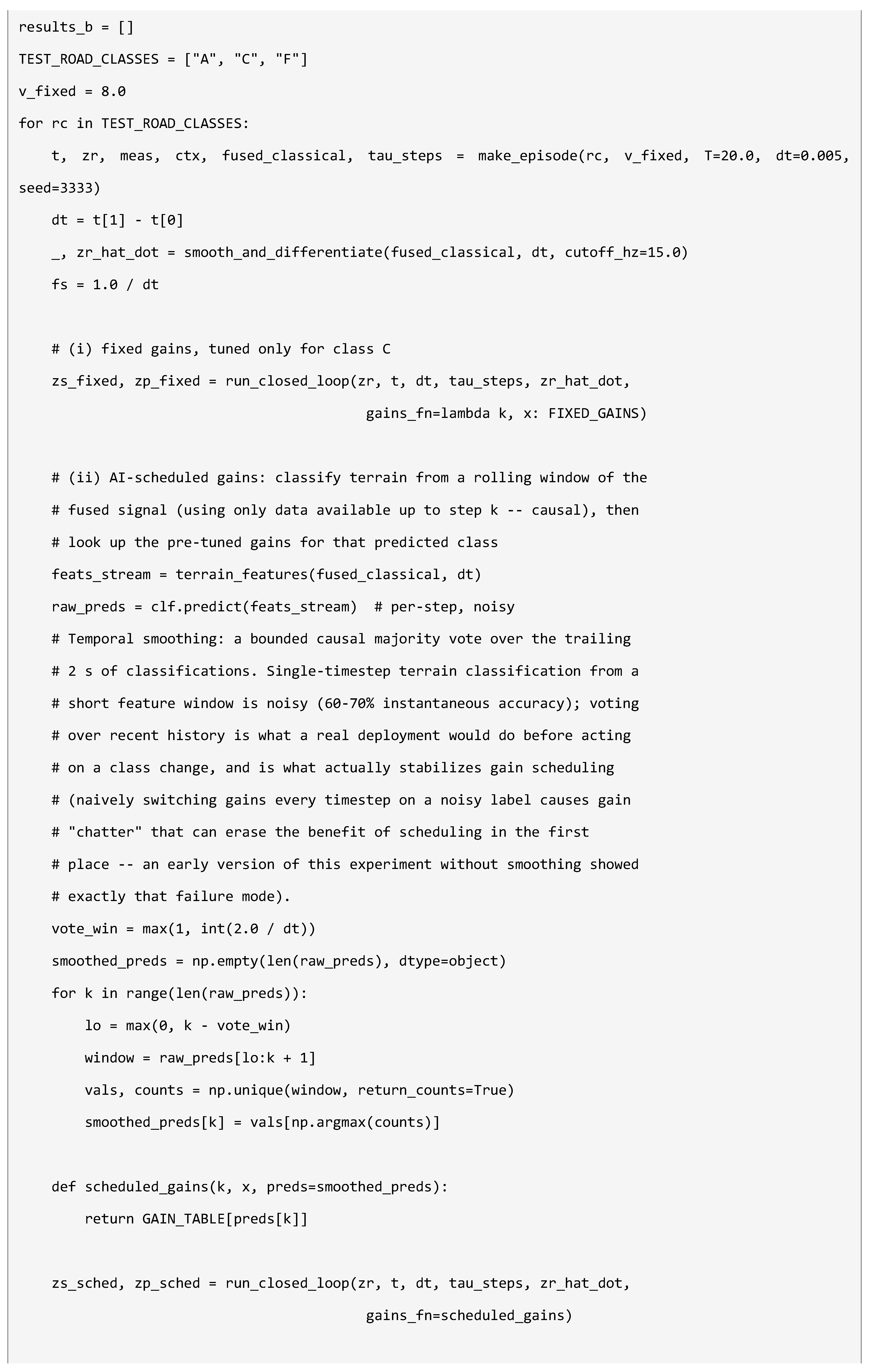
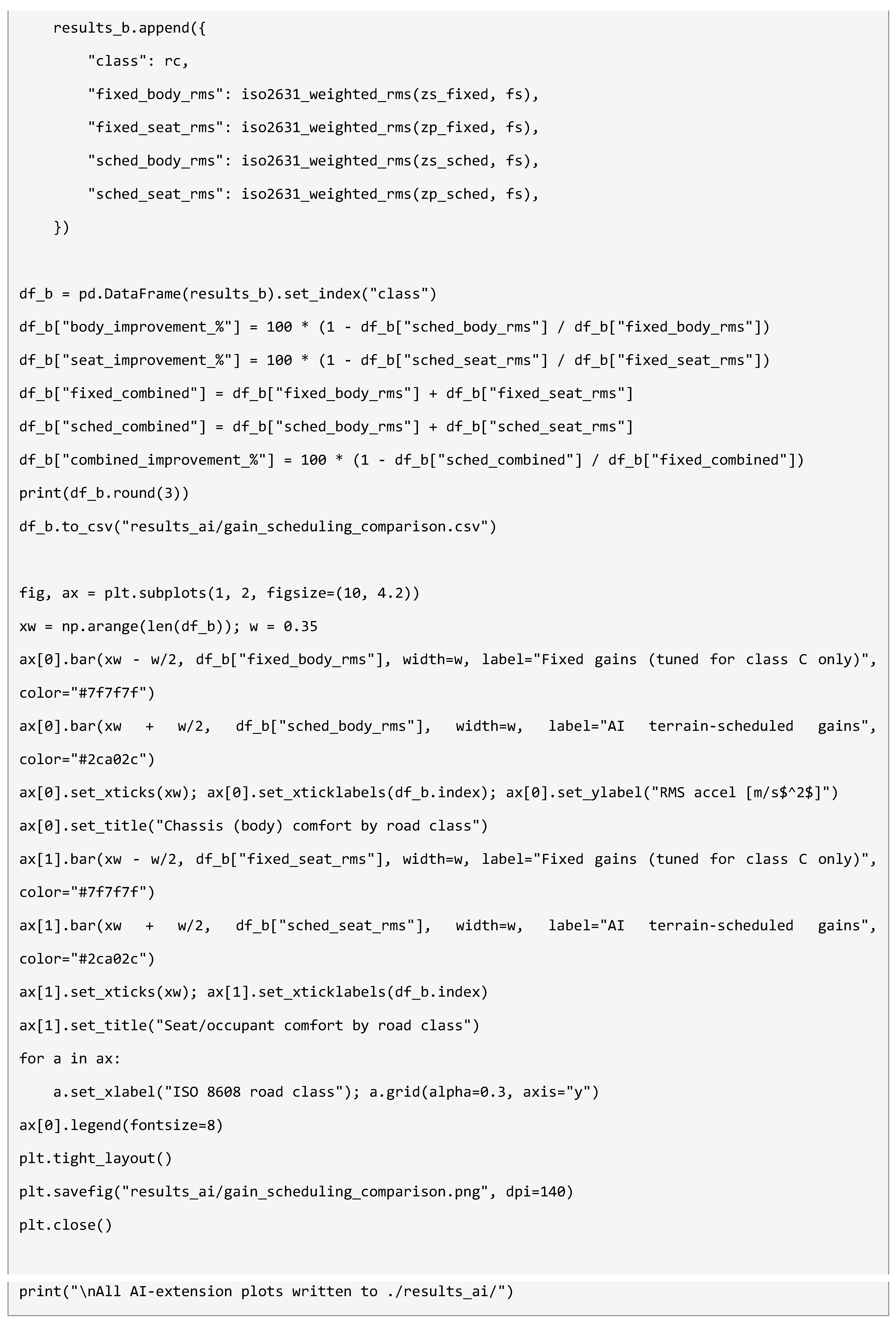
Listing A4. Full contents of run_ai_experiment.py.
References
- ISO 8608:2016, Mechanical Vibration — Road Surface Profiles — Reporting of Measured Data, Int. Org. Standardization, Geneva, Switzerland, 2016.
- ISO 2631-1:1997, Mechanical Vibration and Shock — Evaluation of Human Exposure to Whole-Body Vibration, Int. Org. Standardization, Geneva, Switzerland, 1997.
- D. Karnopp, M. J. Crosby, and R. A. Harwood, “Vibration control using semi-active force generators,” ASME J. Eng. Ind., vol. 96, no. 2, pp. 619–626, 1974. [CrossRef]
- “Machine vision for predictive suspension,” U.S. Patent Appl. 2009/0097038 A1, Apr. 16, 2009.
- “Adaptive active suspension system with road preview,” U.S. Patent 8,996,249 B2 and U.S. Patent Appl. 2014/0195112 A1.
- “Self-driving vehicle with integrated active suspension,” U.S. Patent Appl. 2014/0297116 A1.
- “Suspension control system and method with event detection based on unsprung mass acceleration data and pre-emptive road data,” U.S. Patent Appl. 2022/0281280, Sep. 8, 2022.
- X. Shao, F. Naghdy, H. Du, and Y. Li, “Advances in active suspension systems for road vehicles,” ScienceDirect, 2023.
- “Tesla files patent for predictive suspension using fleet road maps,” Patentlyze, 2026.
- “Active suspension system for vehicle seats,” U.S. Patent 6,059,253 A.
- “Vehicle active suspension control system and method,” U.S. Patent Appl. 2023/0331056, Oct. 19, 2023.
- W. Gong, C. He, K. Su, Q. Li, T. Wu, and Z. J. Wang, “DIDLM: A SLAM dataset for difficult scenarios featuring infrared, depth cameras, LIDAR, 4D radar, and others under adverse weather, low light conditions, and rough roads,” arXiv:2404.09622, 2024.
- “A new dataset and framework for robust road surface classification via camera–IMU fusion,” arXiv:2601.20847, 2026.
- “Low-cost pavement roughness evaluation using inertial measurement unit (IMU)–pulsed coherent radar (PCR) sensor fusion,” ScienceDirect, 2025.
- “Research on vibration reduction performance of electromagnetic active seat suspension based on sliding mode control,” Sensors, vol. 22, no. 15, p. 5916, 2022. [CrossRef]
- L. Breiman, “Random forests,” Mach. Learn., vol. 45, no. 1, pp. 5–32, 2001. [CrossRef]
- F. Pedregosa et al., “Scikit-learn: Machine learning in Python,” J. Mach. Learn. Res., vol. 12, pp. 2825–2830, 2011.
- “Multi-modal assessment of road roughness using smartphone applications, acceleration, and passenger ratings,” arXiv:2606.03427, 2026.
- J. Theunissen, A. Tota, P. Gruber, M. Dhaens, and A. Sorniotti, “Preview-based techniques for vehicle suspension control: A state-of-the-art review,” Annu. Rev. Control, vol. 51, pp. 206–235, 2021. [CrossRef]
- Y. Shen, K. Jing, K. Sun, C. Liu, Y. Yang, and Y. Liu, “Review of uneven road surface information perception methods for suspension preview control,” Sensors, vol. 25, no. 18, p. 5884, 2025. [CrossRef]
Figure 1.
Generic prior-art architecture common to the surveyed systems: forward sensors feed data fusion, which drives a road/suspension estimate, which drives control, closed by a feedback loop from the realized response back into the fusion/estimate stage.
Figure 1.
Generic prior-art architecture common to the surveyed systems: forward sensors feed data fusion, which drives a road/suspension estimate, which drives control, closed by a feedback loop from the realized response back into the fusion/estimate stage.
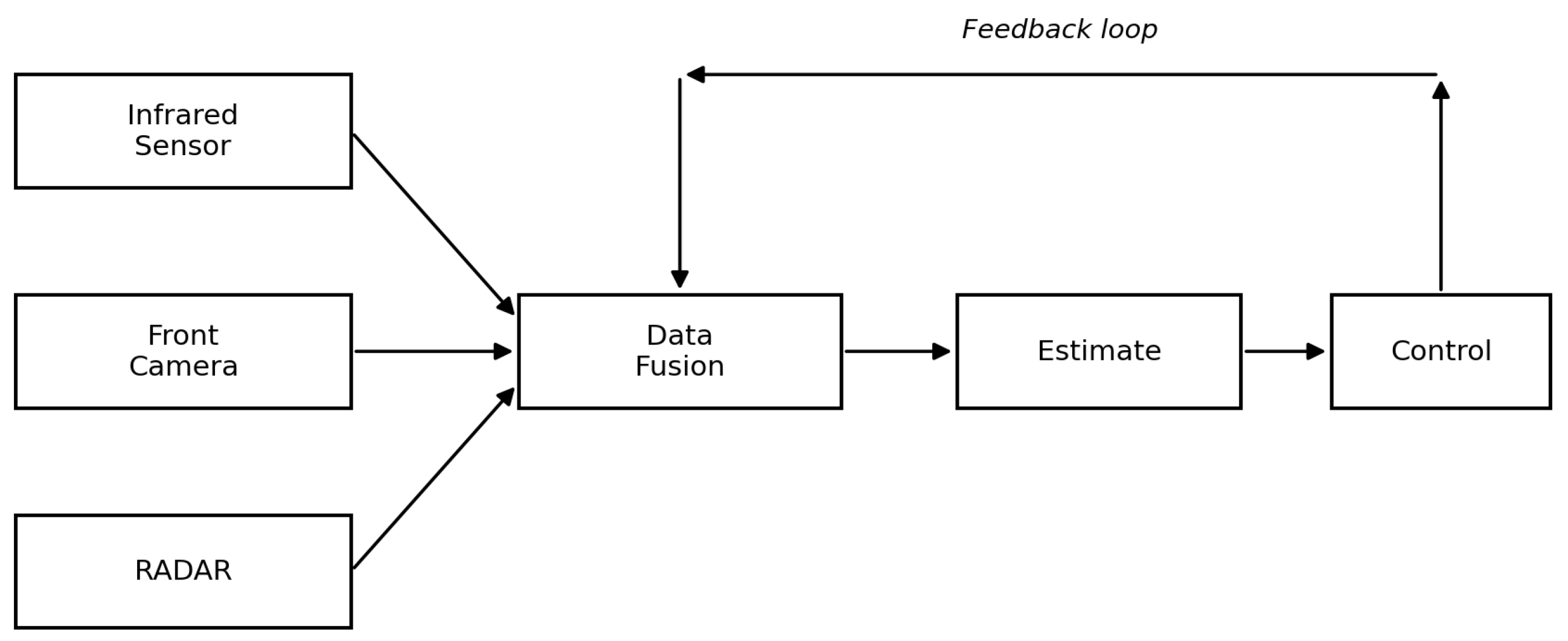
Figure 2.
Proposed system architecture. Sensor fusion (Sections III-B–III-C) and road/suspension estimation (Section III-D) drive a control law (Section III-E) that commands two independently controllable actuators; the realized plant response closes the loop back to the fusion stage as an estimation error signal.
Figure 2.
Proposed system architecture. Sensor fusion (Sections III-B–III-C) and road/suspension estimation (Section III-D) drive a control law (Section III-E) that commands two independently controllable actuators; the realized plant response closes the loop back to the fusion stage as an estimation error signal.
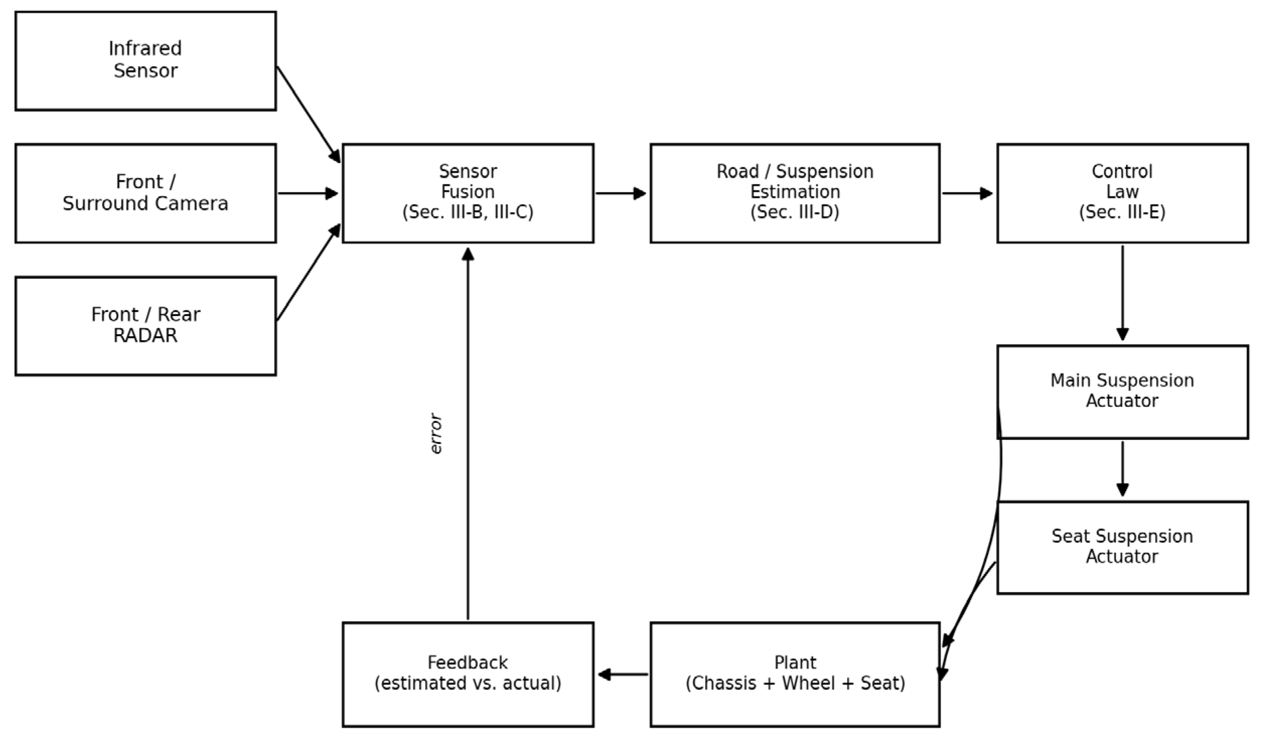
Figure 3.
Physical test-rig data flow. Vehicle sensors and ground-truth instrumentation feed a common data logger; the synchronized dataset is evaluated under all three controller configurations to reproduce the comparison of Section VII.
Figure 3.
Physical test-rig data flow. Vehicle sensors and ground-truth instrumentation feed a common data logger; the synchronized dataset is evaluated under all three controller configurations to reproduce the comparison of Section VII.
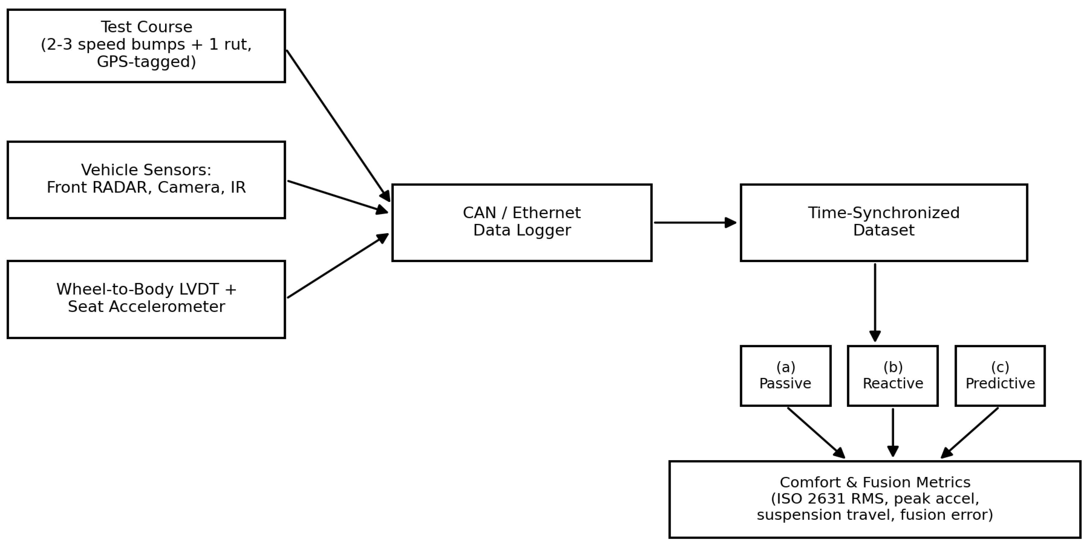
Figure 8.
AI-enhanced pipeline. A learned MLP fusion path (Section VIII-B) runs alongside the classical inverse-variance fusion of Figure 2, and a Random Forest terrain classifier (Section VIII-C) drives a per-class gain table feeding the same control law.
Figure 8.
AI-enhanced pipeline. A learned MLP fusion path (Section VIII-B) runs alongside the classical inverse-variance fusion of Figure 2, and a Random Forest terrain classifier (Section VIII-C) drives a per-class gain table feeding the same control law.
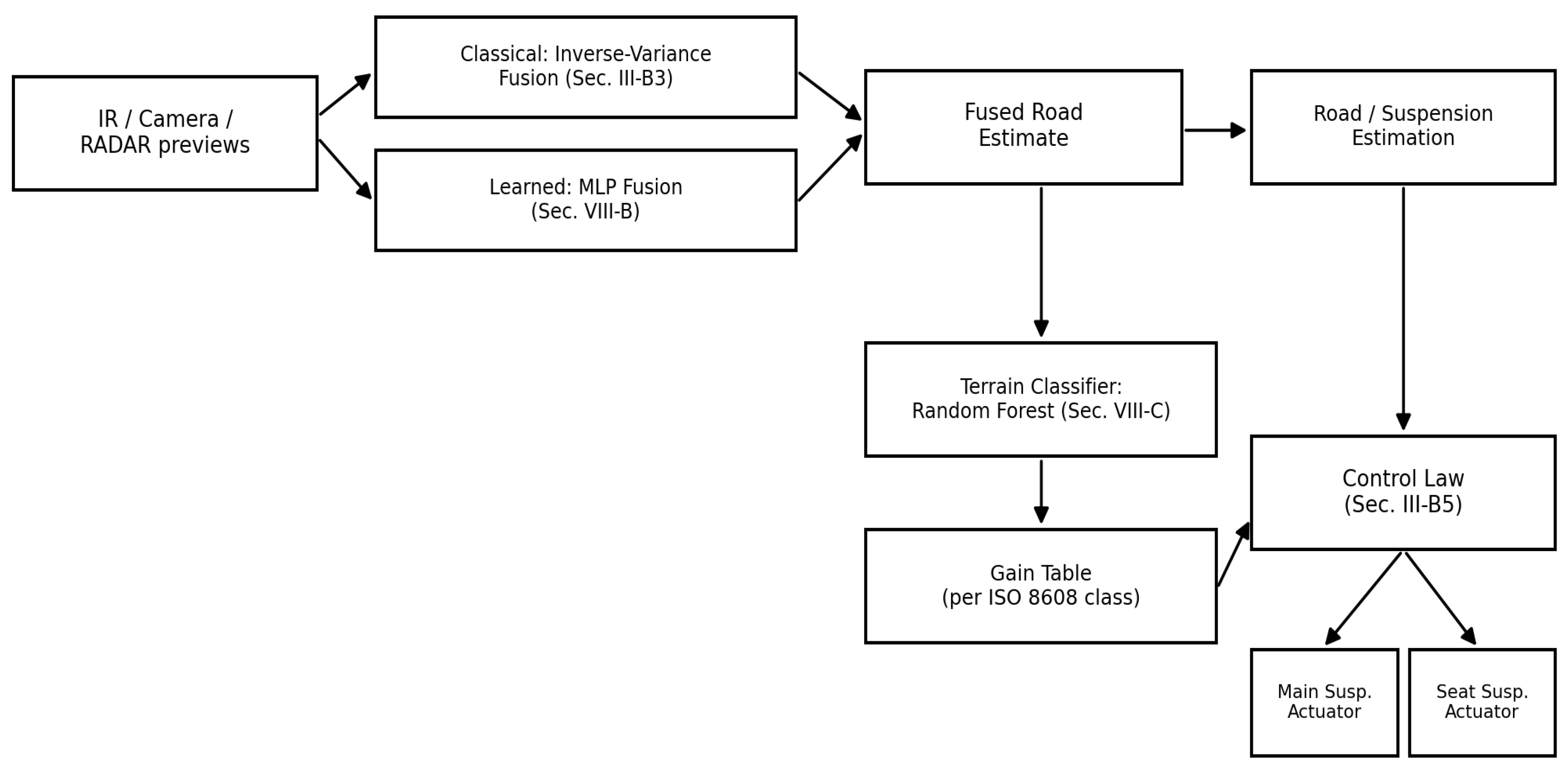
Figure 10.
Terrain (ISO 8608 class) classifier confusion matrix, held-out accuracy 60.7%.
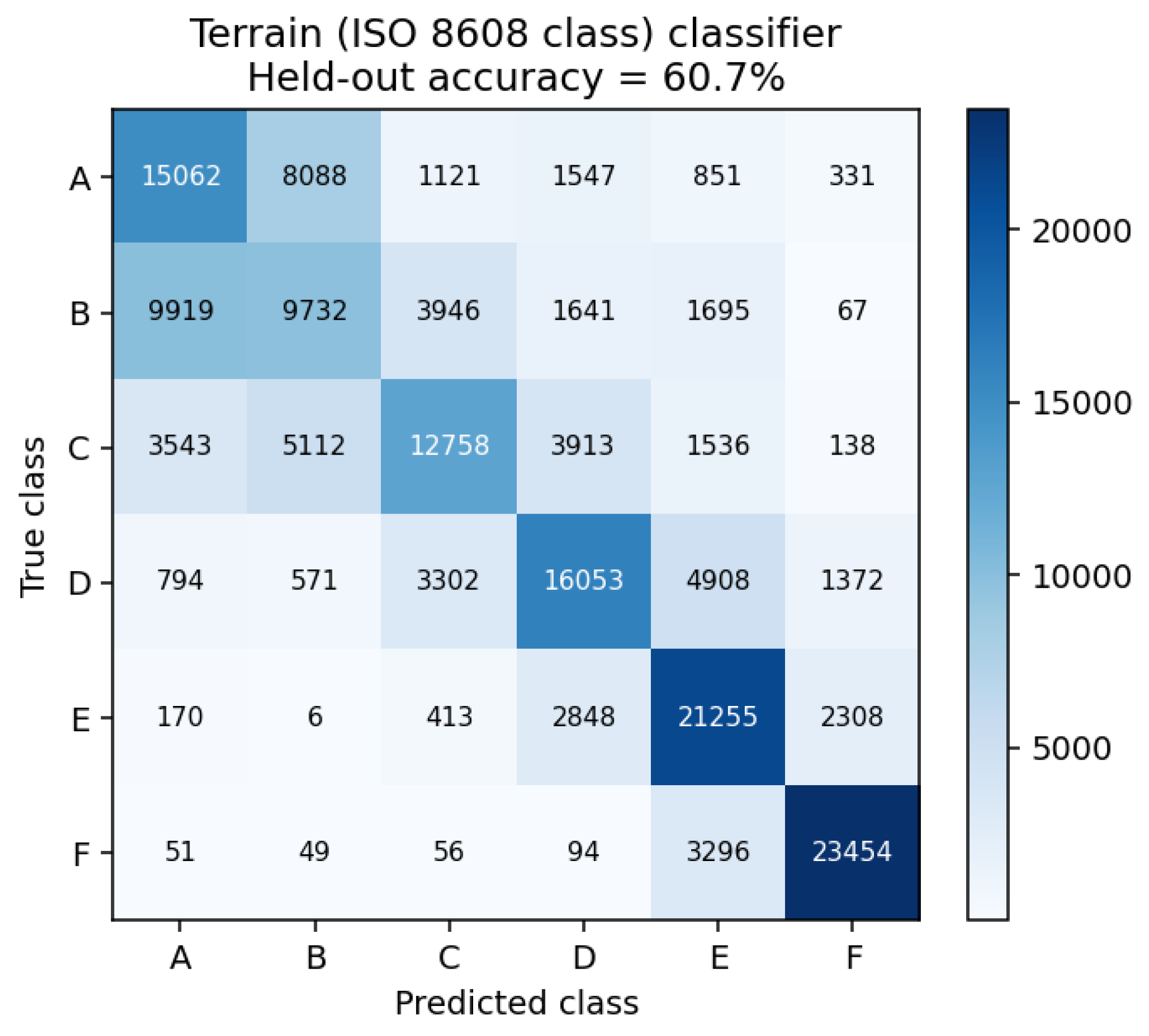
Figure 12.
Prior art produces a claimed mechanism with no accompanying runnable artifact; this work produces the same class of architecture plus an open, independently reproducible implementation and benchmark.
Figure 12.
Prior art produces a claimed mechanism with no accompanying runnable artifact; this work produces the same class of architecture plus an open, independently reproducible implementation and benchmark.
Disclaimer/Publisher’s Note: The statements, opinions and data contained in all publications are solely those of the individual author(s) and contributor(s) and not of MDPI and/or the editor(s). MDPI and/or the editor(s) disclaim responsibility for any injury to people or property resulting from any ideas, methods, instructions or products referred to in the content. |
© 2026 by the authors. Licensee MDPI, Basel, Switzerland. This article is an open access article distributed under the terms and conditions of the Creative Commons Attribution (CC BY) license (http://creativecommons.org/licenses/by/4.0/).
Copyright: This open access article is published under a Creative Commons CC BY 4.0 license, which permit the free download, distribution, and reuse, provided that the author and preprint are cited in any reuse.