

Submitted:
08 August 2026
Posted:
11 August 2026
You are already at the latest version
Abstract
Coffee production and trade are globally important, and Brazil is the world's largest producer and second-largest consumer. However, climate change poses a major challenge to coffee production because the crop is highly sensitive to irregular rainfall distribution and temperature fluctuations. We evaluated temperature and precipitation fluctuations from 1984 to 2023 at two coffee-producing units in southern Minas Gerais, Brazil, to characterize regional climate dynamics and their impacts on coffee yield and total production. We used the Mann–Kendall test and Sen’s slope estimator to identify trends and estimate rates of change in maximum, minimum, and mean air temperature and in total, dry-season, and wet-season precipitation. We used Pearson’s and Spearman’s correlation coefficients to assess relationships between climatic and agronomic variables, selecting the appropriate coefficient based on prior Shapiro–Wilk normality tests. All temperature variables showed warming trends in September, during the transition from the dry to the wet season. Cooling trends were also detected in April, May, and December. At one production unit, dry-season rainfall declined over the historical series. At the other, precipitation declined in May but showed no trend in either the dry or wet season. Relationships between climatic and agronomic variables differed between production units: correlations were positive at one unit and negative at the other. Regionally, these trends indicate vulnerability during critical phenological stages that coincide with these seasonal windows, resulting in pollen tube desiccation, greater consumption of photoassimilates during physiological rest, and poor bean development under reduced dry-season rainfall. The contrasting correlation patterns were attributed to regional climate fluctuations and to the microclimatic, land-use, and land-cover characteristics of each production unit. Under this scenario, mitigating these impacts is essential to minimize damage to coffee crops. Recommended strategies include the implementation of agroforestry systems, rigorous monitoring of pests favored by climate fluctuations, and the adoption of more climate-resilient cultivars. Ultimately, this study highlights that crop management and mitigation strategies designed to buffer these climate impacts must be tailored to the distinct conditions of each production unit.
Keywords:
climate change
; coffee production
; agricultural management
; Arabica coffee
1. Introduction
Coffee is a major global agricultural commodity that supports several strategic sectors, including cultivation, processing, transportation, marketing, and trade, with Brazil playing a leading role [1]. The genus Coffea comprises approximately 130 species, of which C. arabica L. and C. canephora Pierre ex A. Froehner are commercially important [2]. In Brazil, the state of Minas Gerais leads national coffee production, particularly in the South and Southwest mesoregion of Minas Gerais, where a network of cooperatives, exporters, and coffee brokers reinforces the region’s strategic position in domestic and international markets [3,4]. Arabica coffee thrives under favorable edaphoclimatic conditions [5]. Suitable elevations, annual rainfall of 1,200–1,500 mm and temperatures of 15–24 °C are considered ideal for Arabica coffee production, while regular rainfall during the reproductive period is essential [6,7,8]. However, climatic variability poses challenges to coffee cultivation, yield, and total production. High temperatures, drought, hail, and frost events can reduce photosynthetic rates and cause premature flowering, pollen tube desiccation, and flower abortion [9]. These meteorological irregularities may also favor pests as coffee leaf rust (Hemileia vastaris) and infestations by coffee berry borer (Hypothenemus hampei) that are considered the two most important and threatening coffee plants. The losses due to pests account up to 13% annual production worldwide [10,11]. The coffee berry borer is favored by drought periods and high temperatures conditions that have become increasingly frequent [12], whereas higher temperatures and less intense rainfall favor coffee leaf rust, which affects plants grown at higher elevations [13]. Continued warming also reduces land suitability for Arabica coffee [14], potentially making some current production areas unsuitable for cultivation or crop development and increasing the need for new growing areas at higher elevations [15,16].
Against this background, this study analyzed trends and rates of change in temperature and precipitation and their correlations with coffee yield and total production in southern Minas Gerais from 1984 to 2023. We used climate and harvest data provided by Ipanema Coffees (Ipanema Agrícola S.A.) for two production units located in the municipalities of Alfenas and Machado, southern Minas Gerais, Brazil. To this end, we applied the Mann–Kendall test and Sen’s slope estimator, widely used in agrometeorological and environmental analyses, to detect seasonal trends and quantify changes [17,18]. Based on the results of the Shapiro–Wilk normality test, we used Pearson’s or Spearman’s correlation coefficient, as appropriate, to assess the effects of climatic variations on yield and total production [19,20].
2. Materials and Methods
2.1. Study Area and Production Units
We conducted the study at the Conquista and Capoeirinha production units of Ipanema Agrícola S.A., located in the municipalities of Alfenas and Machado, respectively, in southern Minas Gerais, Brazil (Figure 1). The geological substrate of the region consists of gneisses overlain by soils and unconsolidated fluvial deposits of gravel, sand, and clay [24]. Both municipalities are located within the Guaxupé Massif [25]. The region lies within the Atlantic Forest biome, with transition zones to the Cerrado (Brazilian savanna) [26]. Under the Köppen climate classification [27], the region has a humid subtropical climate (Cwb), characterized by dry winters and mild summers, with a mean annual temperature of 21.2 °C and annual precipitation of 1,500–1,750 mm.
The Conquista production unit covers 2,045 ha, comprising 82.26% coffee plantations, 14.54% native forest cover, 1.00% eucalyptus plantations, 0.91% pasture, 0.88% built-up areas and 0.41% of water bodies. The Capoeirinha unit spans 1,772 ha, consisting of 68.07% coffee plantations, 23.08% native forest cover, 5.26% eucalyptus plantations, 1.80% water bodies, 0.93% pasture, and 0.86% built-up areas. Harvesting is fully mechanized at Conquista. At Capoeirinha, 98% of the harvest is mechanized, and the remaining 2% is harvested manually on steep slopes. At Conquista, rows are spaced 3.5–4.0 m apart, with 1.0 m between plants. At Capoeirinha, row spacing is 2.0–4.8 m, and in-row plant spacing is 0.5–2.0 m [28].
2.2. Data Sources and Methodological Overview
The company provided coffee yield (bags/ha), total production (bags), and climate data. Weather stations located at the production units recorded the climate data. The dataset covered 1984–2023 and included mean, maximum, and minimum air temperature; total precipitation; and rainfall during the dry and wet seasons. The methodological workflow used to process and analyze these data is summarized in Figure 2.
2.3. Data Analysis
For trend analyses, both parametric and nonparametric methods can be applied to climate time series. We selected nonparametric methods because they do not assume normally distributed data and are more robust to outliers. Specifically, we applied the Mann–Kendall test to detect trends and Sen’s slope estimator to quantify their magnitude [17]. We processed the data in Python using the pyMannKendall, scikit-learn, and SciPy packages in Visual Studio Code (VS Code).
2.4. Mann–Kendall Test
The Mann–Kendall (MK) test is a nonparametric statistical method developed by Mann [29] and Kendall [30]. It has been widely used to identify increasing and decreasing trends in environmental time series, including temperature, precipitation, and humidity [17,18]. Because autocorrelation can affect the statistical significance of the test, we applied prewhitening to remove the temporal dependence from the data [31]. The MK test does not require normally distributed data and is less sensitive to outliers because it is based on observation ranks rather than absolute values [31,32].
For each time series, the MK test evaluates the null hypothesis () of no trend against the alternative hypothesis () of a monotonic trend. The test statistic S is calculated using Equation (1):
Here, n is the number of observations; xi and xj are the observations at times i and j, respectively, with j > i; and sgn is the sign function defined in Equation (2) [33]:
Positive values of S indicate increasing trends, whereas negative values indicate decreasing trends. The variance of S, corrected for tied observations, is calculated using Equation (3):
Here, m is the number of tied groups, and is the number of observations in the i-th tied group [30].
The standardized Z statistic is calculated from S and Var(S) using Equation (4):
Under the null hypothesis of no trend (H₀), Z follows an approximately standard normal distribution. For the two-sided test, we adopted α = 0.05 and rejected H₀ when p < 0.05.
2.5. Sen’s Slope Estimator
Sen’s slope estimator quantifies trend magnitude as a rate of change in a time series [34]. We used it with the MK test because it is robust to outliers [35]. Pairwise slopes were calculated using Equation (5):
Here, xj and xi are the observations at times j and i, respectively, with j > i, and k indexes each of the N pairwise slopes. For a time series containing n observations, the number of pairwise slopes, N, is calculated using Equation (6):
N = n(n-1)/2
After sorting the N values of in ascending order, we calculated Sen’s slope
() as their median and obtained a 95% confidence interval for the slope estimate. The calculation of Qmed is given by Equation (7):
2.6. Spearman’s Rank Correlation Coefficient
Spearman’s rank correlation coefficient is a nonparametric measure of the strength and direction of the monotonic relationship between two variables. We used it when at least one variable in a pair did not meet the normality assumption. We used this coefficient to identify monotonic, but not necessarily linear, relationships between climatic variables and Arabica coffee yield. In the absence of tied ranks, the coefficient can be calculated from the ranks of paired observations using Equation (8):
Here, is the difference between the ranks assigned to the and for observation i, and n is the number of paired observations. The coefficient ranges from -1 to 1; its sign indicates the direction of the monotonic relationship, and its absolute magnitude indicates its strength. We assessed statistical significance at α = 0.05 [36].
2.7. Pearson’s Correlation Coefficient
Pearson’s correlation coefficient measures the strength and direction of the linear association between two variables. In this study, we used it for variable pairs in which both variables met the normality criterion based on the Shapiro–Wilk test. We used the coefficient to assess whether coffee yield and total production varied linearly with climatic variables. Specifically, we examined whether gradual increases in climatic variables corresponded to increases or decreases in the agronomic variables. This coefficient is calculated as the ratio of the covariance of the variables to the product of their standard deviations, as shown in Equation (9):
Where n is the number of paired observations, and are the observed values of the climatic and agronomic variables, respectively; and and are the corresponding sample means. The coefficient ranges from -1 to 1; its sign indicates the direction of the linear relationship, whereas its absolute value indicates its strength. We assessed statistical significance at α = 0.05 [37].
3. Results
3.1. Trend Analysis of Temperature and Precipitation
We evaluated trends in maximum temperature (), minimum temperature (), and mean temperature (), and precipitation at both production units (Figure 3 and Figure 4) and compared their estimated magnitudes of change (Figure 5). The complete results are provided in Appendices A and B.
Maximum temperature showed significant increasing and decreasing trends, but their occurrence varied among months over the historical time series. At Conquista, Tmax
decreased significantly in April and December, with estimated declines of 3.70 and 2.53 °C over the study period, respectively. In September, Tₘₐₓ increased by 1.84 °C. At Capoeirinha, Tmax decreased significantly in April (2.39 °C), whereas September showed an increase of 2.92 °C, which exceeded the increase at Conquista.
Unlike , generally increased at both production units, although the months and magnitudes differed. At Conquista, Tmin increased in June and September, with estimated increases of 1.82 and 1.93 °C, respectively. At Capoeirinha, increases occurred in more months and were larger: 2.54 °C in June, 2.20 °C in September, and 2.06 °C in October.
showed significant declining trends, except in September, when it increased, consistent with the patterns observed for Tₘₐₓ and Tₘᵢₙ. At Conquista, decreased in April, May, and December, with estimated changes of -2.59, -2.00, and -1.36 °C, respectively. At Capoeirinha, the declines were smaller in April and May, with estimated changes of -1.14 and -1.38 °C, respectively, whereas September showed an estimated increase of 2.34 °C.
We characterized seasonal precipitation patterns using total precipitation accumulated during the dry and wet seasons and monthly precipitation over the historical time series. The complete dataset is provided in Appendix B. In the study region, the dry season extends from April through August, whereas the wet season extends from September through March. Total precipitation at Conquista showed no significant trend. At Capoeirinha, however, May precipitation decreased significantly, with an estimated decline of 34.9 mm over the study period.
Seasonal precipitation trends differed between the production units. At Conquista, wet-season precipitation showed no significant trend, whereas dry-season precipitation declined significantly, with an estimated reduction of 94.7 mm. At Capoeirinha, neither season showed a significant precipitation trend over the historical time series.
3.2. Correlation Analysis
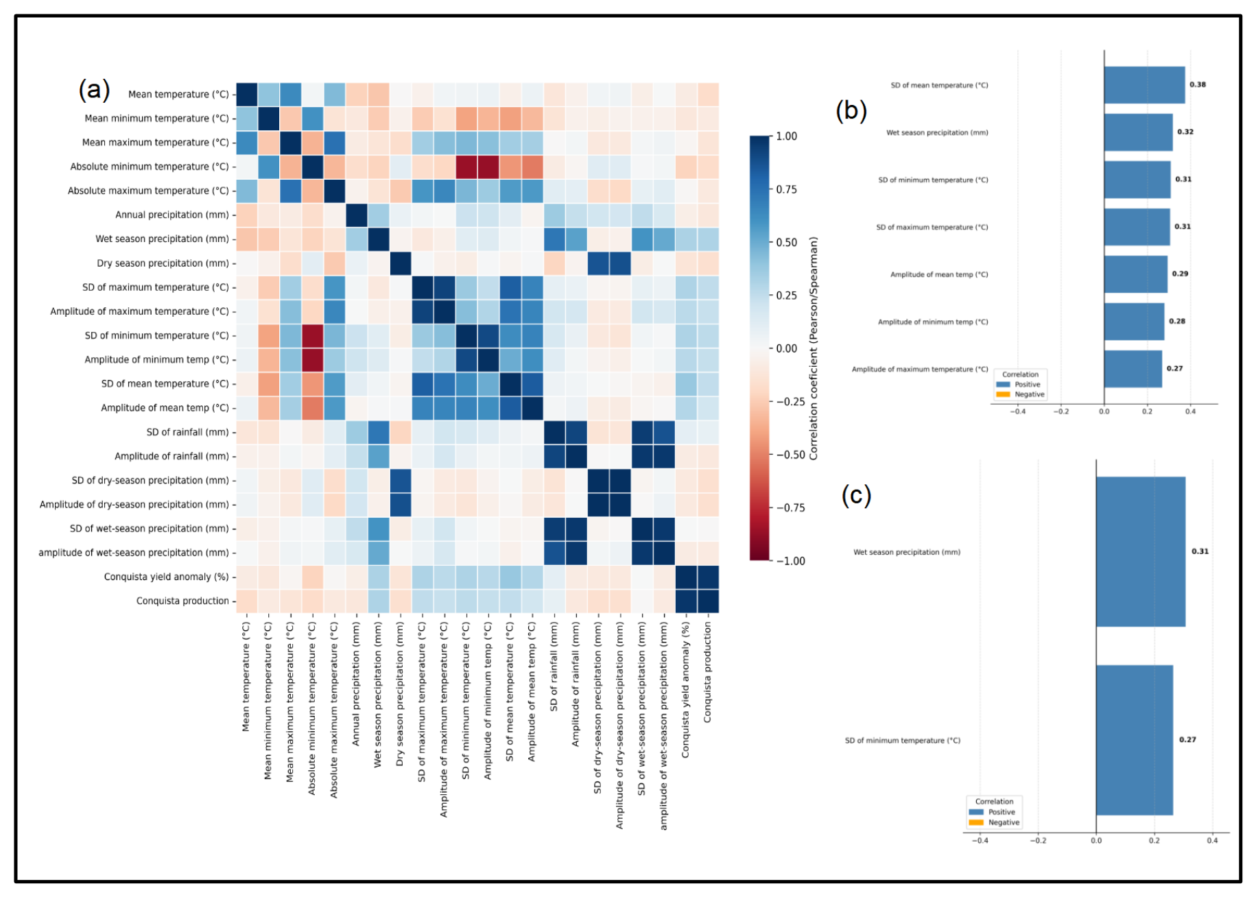
To assess the relationships between climatic and agronomic variables, we constructed a correlation matrix for each production unit. We correlated coffee yield (bags/ha) and total production (bags) with the climatic variables; the results are shown in Figure 6 and Figure 7. In both figures, panel (a) shows the complete correlation matrix, while panels (b) and (c) show selected correlations of climatic variables with coffee yield and total production, respectively.
At the Capoeirinha production unit, the standard deviation and amplitude of dry-season precipitation showed strong negative correlations with both agronomic variables (Figure 6). For coffee yield, the correlation coefficient for the standard deviation of dry-season precipitation was -0.323, while the coefficient for its amplitude was -0.326. The corresponding coefficients for total production were -0.416 and -0.402, respectively.
At the Conquista production unit, the standard deviation of mean temperature and wet-season precipitation were significantly correlated with coffee yield (Figure 7). Their correlation coefficients were 0.376 and 0.318, respectively. The standard deviations of maximum and minimum temperatures, together with the amplitudes of mean, minimum, and maximum temperatures, also showed positive correlations with yield but did not reach statistical significance, although their p-values were close to the significance threshold.
For total production, wet-season precipitation and the standard deviation of minimum temperature approached, but did not reach, statistical significance (p = 0.052 and 0.097, respectively), with corresponding correlation coefficients of 0.308 and 0.265, respectively.
4. Discussion
4.1. Climate Dynamics and Agronomic Variables
Our results reveal significant changes in the climatic profile of both production units over the historical record, characterized by uneven warming, altered rainfall seasonality, and effects on the agronomic variables evaluated. Rates of temperature change in the study areas exceed the mean decadal warming rates projected in IPCC reports. This amplified local climate signal can be attributed to interactions between climate change and local land-use and land-cover change [38,39].
In this context, generally increased, whereas and followed contrasting seasonal patterns, decreasing in the months preceding winter (April and May) and at the onset of summer (December), but increasing markedly in September. Increases in in June and September suggest progressive nocturnal warming. This pattern is consistent with studies of tropical warming, in which increased cloud cover and greenhouse gas concentrations reduce nocturnal longwave heat loss, thereby raising minimum temperatures and narrowing the diurnal temperature range [40,41]. Conversely, the April decreases in (3.70 °C at Conquista and 2.39 °C at Capoeirinha) indicate lower temperature extremes during autumn.
Although the dry and wet seasons are well defined in southern Minas Gerais [42], precipitation showed no significant trends in most months. This overall stability was interrupted by declining rainfall, while the dry season was characterized by high variability. At Capoeirinha, this variability showed strong negative correlations with total production and yield. Together with increasing minimum temperatures in June, this pattern indicates increased evaporation during a period of water scarcity.
Despite being located in the same region, Capoeirinha exhibited greater thermal variability, whereas Conquista was more stable. The strong negative correlations found at Capoeirinha demonstrate the agronomic implications of these patterns. By contrast, proximity to the Furnas Reservoir buffers temperature extremes at Conquista, limiting the rates of change detected by the trend tests [43]. Capoeirinha, in turn, lies within a landscape matrix of diverse croplands, isolated Atlantic Forest fragments, and roads. These landscape features favor warming, unlike the moisture-related buffering effect observed at Conquista [44,45].
4.2. Impacts on Coffee Cultivation in Southern Minas Gerais
Edaphoclimatic conditions, including temperature variability, are key environmental controls on the phenological development and yield of coffee, particularly Arabica coffee. Annual rainfall of 1,200–1,800 mm is considered optimal. Against these requirements, the negative correlations of yield and total production with the standard deviation and amplitude of dry-season rainfall, together with increasing minimum temperatures, provide statistical evidence of adverse effects on both agronomic variables at Capoeirinha. The optimal temperature range is 15–24 °C. Although Arabica coffee can tolerate brief periods of temperature extremes, prolonged exposure to such stress compromises plant physiological performance and yield; temperatures above 34 °C can reduce the photosynthetic rate to near zero [21,46]. Taken together, these ecophysiological requirements and the trends and correlations observed here show that altered temperature and rainfall patterns challenge the phenological development of Arabica coffee and affect both yield and total production [47]. Temperature increases observed in September, immediately following a period of pronounced water stress, make coffee plants vulnerable to irregular flowering and induce flower abortion due to pollen tube desiccation, substantially reducing yield [21].
Declines in and in April and May, combined with lower precipitation during the same period, have contrasting implications for bean maturation and quality. Milder temperatures during ripening prolong the ripening period, favoring the accumulation of carbohydrates and phenolic compounds and improving the sensory attributes of the beverage [48]. This pattern is consistent with the positive correlation found between coffee yield and the standard deviation of at Conquista. Conversely, if the water deficit intensifies, coffee plants may experience preharvest stress and produce malformed beans [49].
The observed increases in in June and September also raise nocturnal respiration in coffee plants. Warmer nights accelerate the consumption of carbohydrates that would otherwise be allocated to branch and fruit growth, leading to early depletion of plant reserves, premature ripening, and greater pressure from pests favored by dry conditions [5,50]. Regular development across phenological stages is critical for coffee yield. Excessive heat in September, coupled with progressively decreasing dry-season rainfall, is a limiting factor that may make coffee cultivation unviable during intense El Niño events, as in 2015 [51]. The ongoing 2026 event is expected to strengthen through the end of the year [51].
4.3. Mitigation Strategies
Reducing greenhouse gas emissions is fundamental to mitigating climate change and its impacts. On-farm activities in coffee production are substantial sources of nitrous oxide (), carbon dioxide (), and methane () emissions resulting from fossil fuel consumption, electricity use, firewood combustion, and, particularly, nitrogen fertilizer application and liming [28,52,53]. In this context, incorporating trees into coffee plantations and maintaining forested areas within production units are effective management strategies for mitigating future impacts on coffee crops.
Trees sequester carbon, while shade provides microclimatic benefits for Arabica coffee [54]. The use of fertilizers containing urease and nitrification inhibitors is also an important mitigation measure [55].
Climate forecasting based on weather-station data supports temporal analyses of precipitation and temperature, informs strategic decision-making in response to climate change, and facilitates the development of models and projections [56]. Alongside these strategies, advances in genomics and transcriptional regulation are also important. Because small RNAs (sRNAs) respond to environmental signals and regulate gene expression, they may provide tools for developing coffee plants with greater tolerance to climate-related stress [57].
4.4. Limitations
First, we controlled serial autocorrelation by applying prewhitening before the MK test to ensure the robustness of the detected trends in this study. However, Sen’s slope estimator assumes a linear and monotonic trend over time. It may therefore not fully capture nonlinear climatic fluctuations or abrupt shifts in the historical time series.
Second, although the study provides significant insights into climate dynamics and their ecophysiological implications for Arabica coffee, the analysis relies on historical weather-station records. Although these records are highly reliable, they may not fully capture site-specific microclimatic variation at Conquista and Capoeirinha.
Finally, the physiological effects discussed for coffee plants, including flower abortion and the depletion of carbohydrate reserves, were inferred from physiological mechanisms described in the literature rather than measured directly in this study. Future studies integrating automated microclimate sensors with crop models could refine the projections presented here.
5. Conclusions
Overall, the trend analyses and their estimated rates of change revealed marked climate variability across the study area. Increasing and decreasing trends occurred throughout the historical record, and their magnitudes differed between the production units and exceeded the decadal warming rates reported by the IPCC. Capoeirinha showed greater variability, whereas Conquista was more stable. The correlation analyses also produced contrasting results that were consistent with the trend analyses and estimated rates of change.
Global-scale assessments can smooth climatic extremes because they integrate extensive oceanic and vegetated areas, whereas the landscape characteristics surrounding Capoeirinha act as local risk factors. By contrast, Conquista is adjacent to the Furnas Reservoir, whose thermal buffering effect was reflected in the smaller rates of change detected by the trend tests.
This study demonstrated that climate-related effects differed between the two production units. Therefore, management and mitigation strategies should be site-specific and tailored to the conditions at each production unit.
Supplementary Materials
Th This study analyzed trends and rates of change in temperature and precipitation and their correlations with coffee yield and total production in southern Minas Gerais from 1984 to 2023. To do so, we used climate and harvest data provided by Ipanema Coffees (Ipanema Agrícola S.A.) for production units of Conquista and Capoeirinha, located respectively the municipalities of Alfenas and Machado, southern Minas Gerais, Brazil. Therefore, we apply the Mann–Kendall test and Sen’s slope estimator to detect seasonal trends and quantify changes. The following supporting information can be downloaded at the website of this paper posted on Preprints.org, Figure S1: title; Table S1: title; Video S1: title.
Author Contributions
Conceptualization, F.S.G., F.G.R., G.S.R., J.E.B.A., V.S. and R.L.M.; methodology, F.S.G., F.G.R., G.S.R., J.E.B.A., V.S. and R.L.M.; software, F.S.G. J.E.B.A and P.F.R.G; validation, F.S.G.; formal analysis, F.S.G. F.G.R and R.L.M.; investigation, F.S.G, F.G.R, J.E.B.A and R.L.M.; resources, A.R.C.N., R.L.M. and V.S.; data curation, B.R.S., D.O. and L.B.Z and P.F.R.G; writing—original draft preparation, F.S.G.; writing—review and editing, F.S.G., F.G.R., G.S.R., J.E.B.A., V.S. and R.L.M.; visualization, F.S.G.; supervision, A.R.C.N., F.G.R and R.L.M; project administration, F.S.G. and R.L.M.; funding acquisition, A.R.C.N., R.L.M. and V.S. All authors have read and agreed to the published version of the manuscript.
Funding
This research was funded by the Coordination for the Improvement of Higher Education Personnel—Brazil (CAPES), Finance Code 001. The APC was funded by the authors Antonio Rodrigues da Cunha Neto, Velibor Spalevic and Ronaldo Luiz Mincato.
Data Availability Statement
The data can be made available upon request to the authors.
Acknowledgments
The authors thank CAPES (Coordination for the Improvement of Higher Education Personnel) for scholarships awarded to F.S.G. and G.S.R, and CNPq (National Council for Scientific and Technological Development) for the scholarship awarded to L.B.Z. .
Conflicts of Interest
The authors declare no conflicts of interest.
Appendix A

Table A1.
Temperature trend analysis results for the Conquista production unit.
| Conquista—maximum temperature | ||||
| Month | Trend | p-value |
Sen’s slope (°C year⁻¹) |
Estimated change (°C) |
| Jan | No trend | 0.1754 | -0.0547 | -2.180 |
| Feb | No trend | 0.0903 | -0.0609 | -2.436 |
| Mar | No trend | 0.0815 | -0.0574 | -2.296 |
| Apr | Decreasing | 0.001 | -0.0925 | -3.703 |
| May | No trend | 0.1158 | -0.0525 | -2.10 |
| Jun | No trend | 0.6632 | -0.0097 | -0.388 |
| Jul | No trend | 0.3837 | 0.0010 | 0.04 |
| Aug | No trend | 0.5452 | 0.0001 | 0.004 |
| Sep | Increasing | 0.0147 | 0.0461 | 1.84 |
| Oct | No trend | 0.7715 | -0.0281 | -1.124 |
| Nov | No trend | 0.069 | -0.0610 | -2.440 |
| Dec | Decreasing | 0.0118 | -0.0633 | -2.532 |
| Conquista—minimum temperature | ||||
| Month | Trend | p-value |
Sen’s slope (°C year⁻¹) |
Estimated change (°C) |
| Jan | No trend | 0.3579 | -0.006 | -0.248 |
| Feb | No trend | 0.1910 | -0.0161 | -0.644 |
| Mar | No trend | 0.9133 | 0 | 0 |
| Apr | No trend | 0.2172 | -0.0038 | -0.152 |
| May | No trend | 0.2175 | -0.0302 | -1.208 |
| Jun | Increasing | 0.0294 | 0.0456 | 1.824 |
| Jul | No trend | 0.6457 | 0 | 0 |
| Aug | No trend | 0.9229 | 0 | 0 |
| Sep | Increasing | 0.0089 | 0.0483 | 1.932 |
| Oct | No trend | 0.1605 | 0.0248 | 0.99 |
| Nov | No trend | 1 | -0.003 | -0.120 |
| Dec | No trend | 0.4679 | 0.002 | 0.080 |
| Conquista—mean temperature | ||||
| Month | Trend | p-value |
Sen’s slope (°C year⁻¹) |
Estimated change (°C) |
| Jan | No trend | 0.0950 | -0.0345 | -1.380 |
| Feb | No trend | 0.1534 | -0.0371 | -1.480 |
| Mar | No trend | 0.0529 | -0.0341 | -1.364 |
| Apr | Decreasing | 0.00013 | -0.0649 | -2.59 |
| May | Decreasing | 0.01107 | -0.0500 | -2.00 |
| Jun | No trend | 0.0696 | 0.0166 | 0.664 |
| Jul | No trend | 0.2172 | 0.0092 | 0.368 |
| Aug | No trend | 0.7166 | 0.0054 | 0.216 |
| Sep | No trend | 0.0643 | 0.0244 | 0.976 |
| Oct | No trend | 0.4679 | 0.0064 | 0.256 |
| Nov | No trend | 0.0559 | -0.0347 | -1.388 |
| Dec | Decreasing | 0.0374 | -0.0342 | -1.368 |
Table A2.
Temperature trend analysis results for the Capoeirinha production unit.
| Capoeirinha—maximum temperature | ||||
| Month | Trend | p-value |
Sen’s slope (°C year⁻¹) |
Estimated change (°C) |
| Jan | No trend | 0.9421 | 0 | 0 |
| Feb | No trend | 0.8465 | -0.0217 | -0.868 |
| Mar | No trend | 0.8655 | -0.0114 | -0.456 |
| Apr | Decreasing | 0.0083 | -0.0597 | -2.390 |
| May | No trend | 0.1050 | -0.0538 | -2.152 |
| Jun | No trend | 0.7531 | -0.0346 | -1.384 |
| Jul | No trend | 0.8845 | -0.0136 | -0.544 |
| Aug | No trend | 0.6284 | 0.0345 | 1.380 |
| Sep | Increasing | 0.0472 | 0.0731 | 2.921 |
| Oct | No trend | 0.7901 | 0.0039 | 0.153 |
| Nov | No trend | 0.8276 | -0.0140 | -0.560 |
| Dec | No trend | 0.5452 | 0.0120 | 0.480 |
| Capoeirinha—minimum temperature | ||||
| Month | Trend | p-value |
Sen’s slope (°C year⁻¹) |
Estimated change (°C) |
| Jan | No trend | 0.0559 | 0.0307 | 1.228 |
| Feb | No trend | 0.4532 | 0.0105 | 0.420 |
| Mar | No trend | 0.2358 | 0.0235 | 0.940 |
| Apr | No trend | 0.5779 | 0.001 | 0.04 |
| May | No trend | 0.8276 | -0.0084 | -0.336 |
| Jun | Increasing | 0.0031 | 0.0634 | 2.543 |
| Jul | No trend | 0.3212 | 0.0170 | 0.680 |
| Aug | No trend | 0.3212 | 0.0139 | 0.556 |
| Sep | Increasing | 0.0127 | 0.0549 | 2.200 |
| Oct | Increasing | 0.0118 | 0.0515 | 2.060 |
| Nov | No trend | 0.1605 | 0.0333 | 1.332 |
| Dec | No trend | 0.0696 | 0.0294 | 1.176 |
| Capoeirinha—mean temperature | ||||
| Month | Trend | p-value |
Sen’s slope (°C year⁻¹) |
Estimated change (°C) |
| Jan | No trend | 0.5293 | 0.0097 | 0.388 |
| Feb | No trend | 0.6114 | 0 | 0 |
| Mar | No trend | 0.6632 | 0.0036 | 0.144 |
| Apr | Decreasing | 0.0421 | -0.0284 | -1.140 |
| May | Decreasing | 0.0244 | -0.0347 | -1.388 |
| Jun | No trend | 0.1050 | 0.0150 | 0.600 |
| Jul | No trend | 0.6986 | 0.0022 | 0.088 |
| Aug | No trend | 0.3095 | 0.0223 | 0.892 |
| Sep | Increasing | 0.0089 | 0.0589 | 2.340 |
| Oct | No trend | 0.1534 | 0.0281 | 1.124 |
| Nov | No trend | 0.3971 | 0.0128 | 0.512 |
| Dec | No trend | 0.1052 | 0.0194 | 0.776 |
Appendix B
Table B1.
Precipitation trend analysis results for the dry and wet seasons at the two production units.
Table B1.
Precipitation trend analysis results for the dry and wet seasons at the two production units.
| Conquista | |||||||
| Season | Trend | p-value |
Sen’s slope (mm year⁻¹) |
Estimated change (mm) | |||
| Dry | Decreasing | 0.0329 | -2.367 | -94.7 | |||
| Wet | No trend | 0.6495 | 1.43 | 57.2 | |||
| Capoeirinha | |||||||
| Season | Trend | p-value |
Sen’s slope (mm year⁻¹) |
Estimated change (mm) | |||
| Dry | No trend | 0.3579 | -0.006 | -0.248 | |||
| Wet | No trend | 0.1910 | -0.0161 | -0.644 | |||
Table B2.
Monthly precipitation trend analysis results for the two production units.
| Conquista | ||||||
| Month | Trend | p-value |
Sen’s slope (mm year⁻¹) |
Estimated change (mm) | ||
| Jan | No trend | 0.8465 | 0.5549 | 22.196 | ||
| Feb | No trend | 0.9198 | 0.1789 | 7.156 | ||
| Mar | No trend | 0.9421 | 0.6517 | 26.068 | ||
| Apr | No trend | 0.1336 | -0.8052 | -32.208 | ||
| May | No trend | 0.2870 | -0.3727 | -14.908 | ||
| Jun | No trend | 0.1158 | 0.2500 | 10.000 | ||
| Jul | No trend | 0.0624 | -0.2356 | -9.424 | ||
| Aug | No trend | 0.3331 | -0.0831 | -3.324 | ||
| Sep | No trend | 0.4065 | -0.4500 | -18.000 | ||
| Oct | No trend | 0.8088 | 0.0424 | 1.696 | ||
| Nov | No trend | 0.0815 | 1.2923 | 51.692 | ||
| Dec | No trend | 0.2083 | -1.4740 | -58.960 | ||
| Capoeirinha | ||||||
| Month | Trend | p-value |
Sen’s slope (mm year⁻¹) |
Estimated change (mm) | ||
| Jan | No trend | 0.7348 | 1.0738 | 42.952 | ||
| Feb | No trend | 0.9037 | 0.3615 | 14.460 | ||
| Mar | No trend | 0.7166 | 0.0320 | 1.280 | ||
| Apr | No trend | 0.3095 | -0.6125 | -24.500 | ||
| May | Decreasing | 0.0189 | -0.8744 | -34.9 | ||
| Jun | No trend | 0.1158 | 0.4404 | 17.616 | ||
| Jul | No trend | 0.2657 | -0.1267 | -5.068 | ||
| Aug | No trend | 0.3212 | 0.0881 | 3.524 | ||
| Sep | No trend | 0.1914 | -0.7721 | -30.884 | ||
| Oct | No trend | 0.1534 | 1.6968 | 67.872 | ||
| Nov | No trend | 0.0773 | 1.4489 | 57.956 | ||
| Dec | No trend | 0.7348 | 0.8742 | 34.698 | ||
References
- Conab. Companhia Nacional de Abastecimento: Acompanhamento da safra brasileira de café; Brasília, DF, 2026; Volume 13. [Google Scholar]
- Davis, A.P.; Rakotonasolo, F. Six New Species of Coffee (Coffea) from Northern Madagascar. Kew Bull. 2021, 76, 497–511. [Google Scholar] [CrossRef]
- ICO—International Coffee Organization. ICO Coffee Year Production by Country: Coffee Market Report. 2018. Available online: https://ico.org/what-we-do/world-coffee-statistics-database/ (accessed on 25 January 2025).
- CONAB-Companhia Nacional de Abastecimento: Acompanhamento da safra brasileira de café. Brasília DF 2025, 12.
- Magrach, A.; Ghazoul, J. Climate and Pest-Driven Geographic Shifts in Global Coffee Production: Implications for Forest Cover, Biodiversity and Carbon Storage. PLoS ONE 2015, 10, e0133071. [Google Scholar] [CrossRef] [PubMed]
- Legesse, A. Climate Change Effect on Coffee Yield and Quality: A Review. Int. J. For. Hortic. 2019, 5. [Google Scholar] [CrossRef]
- Mangal, S. K. Coffee: planting, production, and processing; Gene-Tech Books: New Delhi, 2007; 1 recurso online (368 p.). [Google Scholar]
- Camargo, Â.P.D.; Camargo, M.B.P.D. Definição e esquematização das fases fenológicas do cafeeiro arábica nas condições tropicais do Brasil. Bragantia 2001, 60, 65–68. [Google Scholar] [CrossRef]
- Santos, C.; Leitao, A.; Pais, I.; Lidon, F.; Ramalho, J. Perspectives on the Potential Impacts of Climate Changes on Coffee Plant and Bean Quality. Emir. J. Food Agric. 2015, 27, 152. [Google Scholar] [CrossRef]
- Ogundeji, B.A.; Olalekan-Adeniran, M.A.; Orimogunje, O.A.; Awoyemi, S.O.; Yekini, B.A.; Adewoye, G.A.; Bankole, I.A. Climate Hazards and the Changing World of Coffee Pests and Diseases in Sub-Saharan Africa. JEAI 2019, 1–12. [Google Scholar] [CrossRef]
- Agegnehu, E.; Thakur, A.; Mulualem, T. Potential Impact of Climate Change on Dynamics of Coffee Berry Borer (Hypothenemus Hampi Ferrari) in Ethiopia. OALib 2015, 02, 1–11. [Google Scholar] [CrossRef]
- Laurentino, E.; Medeiros Costa, J.N. Descrição e caracterização biológica da broca-do-café (Hypothenemus hampei, Ferrari 1867) no Estado de Rondônia / Eliane Laurentino, José Nilton Medeiros Costa; Embrapa Rondônia: Porto Velho, 2004. [Google Scholar]
- Ebisa, D.B. Impacts of Climate Change on Global Coffee Production Industry: Review. Afr. J. Agric. Res. 2017, 12, 1607–1611. [Google Scholar] [CrossRef]
- Getachew, W.M.; Demelash, T. The Impact of Climate Change on Coffee (Coffea Arabica L.) Production and Genetic Resources. Int. J. Res. Stud. Agric. Sci. 2019, 5. [Google Scholar] [CrossRef]
- Davis, A.P.; Gole, T.W.; Baena, S.; Moat, J. The Impact of Climate Change on Indigenous Arabica Coffee (Coffea Arabica): Predicting Future Trends and Identifying Priorities. PLoS ONE 2012, 7, e47981. [Google Scholar] [CrossRef] [PubMed]
- Ovalle-Rivera, O.; Läderach, P.; Bunn, C.; Obersteiner, M.; Schroth, G. Projected Shifts in Coffea Arabica Suitability among Major Global Producing Regions Due to Climate Change. PLoS ONE 2015, 10, e0124155. [Google Scholar] [CrossRef] [PubMed]
- Chandler, R.N.; Scott, M. Statistical Methods for Trend Detection and Analysis in the Environmental Sciences, First Edition. 2011. [Google Scholar] [CrossRef]
- Bombardi, R.J.; Carvalho, L.M.V.D. Práticas Simples em Análises Climatológicas: Uma Revisão. Rev. bras. meteorol. 2017, 32, 311–320. [Google Scholar] [CrossRef]
- Souza, R.R.; Toebe, M.; Mello, A.C.; Bittencourt, K.C. Sample size and Shapiro-Wilk test: An analysis for soybean grain yield. Eur. J. Agron. 2022, 141, 126666. [Google Scholar] [CrossRef]
- Rebekić, A.; Lončarić, Z.; Petrović, S.; Marić, S. PEARSON’S OR SPEARMAN’S CORRELATION COEFFICIENT—WHICH ONE TO USE? Poljoprivreda 2015, 21, 47–54. [Google Scholar] [CrossRef]
- DaMatta, F.M.; Ronchi, C.P.; Maestri, M.; Barros, R.S. Ecophysiology of Coffee Growth and Production. Braz. J. Plant Physiol. 2007, 19, 485–510. [Google Scholar] [CrossRef]
- Xiao, W.; Boucher, S.R.; Sexton, R.J. Local Conditions Matter: Climate Change and Coffee Production in Brazil. Clim. Change 2025, 178, 183. [Google Scholar] [CrossRef]
- Silva, J.B.C.D.; Pinto, P.A.L.D.A. Impactos socioeconômicos das mudanças climáticas na produção do café: uma revisão sistemática da literatura. RBClima 2024, 35, 155–178. [Google Scholar] [CrossRef]
- Silva, M. A.; Pinto, C.P.; Pinheiro, M.A.P.; Marinho, M.S.; Lombello, J.C.; Pinho, J.M.M.; Goulart, L.E.A.; Magalhães, J.R. Mapa geológico do estado de Minas Gerais 1 mapa, color. Escala 1:1.000.000; CPRM: Belo Horizonte, 2020. [Google Scholar]
- Hasui, Y. A Grande colisão pré-cambriana do sudeste brasileiro e a estruturação regional. Geociências 2010, 29(2), 141–169. [Google Scholar]
- Ribeiro, A. Geologia e recursos minerais da folha Alfenas SF.23-V-D-I:escala 1:100.000, estado de Minas Gerais. In Escala 1:100.000.; CPRM, UFRJ: Rio de Janeiro, 2020. [Google Scholar]
- Alvares, C.A.; Stape, J.L.; Sentelhas, P.C.; Gonçalves, J.L.M.; Sparovek, G. Köppen’s climate classification map for Brazil. Meteorol. Z. 2013, 22, 711–728. [Google Scholar] [CrossRef] [PubMed]
- Santana, D.B.; Rios, G.D.S.; Lense, G.H.E.; Rubira, F.G.; Franceschi, F.R.A.; Spalevic, V.; Ayer, J.E.B.; Mincato, R.L. Soil and Organic Carbon Losses by Water Erosion in Coffee-Growing Areas in Southern Minas Gerais, Brazil. Turk. J. Agric. For. 2024, 48, 317–331. [Google Scholar] [CrossRef]
- Mann, Henry B. Nonparametric Tests Against Trend. Econometrica 13, 245–59. [CrossRef]
- Kendall, M. G. Rank Correlation Methods; Griffin: London, 1975. [Google Scholar]
- Sonali, P.; Nagesh Kumar, D. Review of Trend Detection Methods and Their Application to Detect Temperature Changes in India. J. Hydrol. 2013, 476, 212–227. [Google Scholar] [CrossRef]
- Jiqin, H.; Gelata, F.T.; Chaka Gemeda, S. Application of MK Trend and Test of Sen’s Slope Estimator to Measure Impact of Climate Change on the Adoption of Conservation Agriculture in Ethiopia. J. Water Clim. Change 2023, 14, 977–988. [Google Scholar] [CrossRef]
- Wilks, D.S. Statistical Methods in the Atmospheric Sciences; Academic Press: Burlington, MA 01803, 2011; Volume 2, pp. 156–162. [Google Scholar]
- Aditya, F.; Gusmayanti, E.; Sudrajat, J. Rainfall Trend Analysis Using Mann-Kendall and Sen’s Slope Estimator Test in West Kalimantan. IOP Conf. Ser. Earth Environ. Sci. 2021, 893, 012006. [Google Scholar] [CrossRef]
- Sen, P.K. Estimates of the regression coefficient based on Kendall’s tau. J. Am. Stat. Assoc. 1968, 63, 1379–1389. [Google Scholar] [CrossRef]
- Corder, G.W.; Foreman, V.D. Nonparametric Statistics: A Step-by-Step Approach; John Wiley & Sons: Hoboken, NJ, USA, 2014. [Google Scholar]
- Steel, R.G.D.; Torrie, J.H.; Dickey, D.A. Principles and Procedures of Statistics: A Biometrical Approach, 3rd ed.; McGraw-Hill: New York, NY, USA, 1997. [Google Scholar]
- Calvin, K.; Dasgupta, D.; Krinner, G.; Mukherji, A.; Thorne, P.W.; Trisos, C.; Romero, J.; Aldunce, P.; Barrett, K.; Blanco, G.; et al. IPCC, 2023: Climate Change 2023: Synthesis Report. Contribution of Working Groups I, II and III to the Sixth Assessment Report of the Intergovernmental Panel on Climate Change. In IPCC, First.; Lee, H., Romero, J., et al., Eds.; Intergovernmental Panel on Climate Change (IPCC): Geneva, Switzerland, 2023. [Google Scholar]
- Pachauri, R.K.; Mayer, L.; Change, Intergovernmental Panel on Climate (Eds.) Climate Change 2014: Synthesis Report; Intergovernmental Panel on Climate Change: Geneva, Switzerland, 2015; ISBN 978-92-9169-143-2. [Google Scholar]
- Robinson, A.; Lehmann, J.; Barriopedro, D.; Rahmstorf, S.; Coumou, D. Increasing Heat and Rainfall Extremes Now Far Outside the Historical Climate. npj Clim. Atmos. Sci. 2021, 4, 45. [Google Scholar] [CrossRef]
- Carter, A.W.; Fleming, J.M. Hotter Nights, Hidden Consequences: An Overlooked Dimension of Climate Change. Integr. Comp. Biol. 2025, 65, 832–849. [Google Scholar] [CrossRef] [PubMed]
- Reis, A.L.; Silva, M.S.; Regis, M.V.; Da Silveira, W. W.; De Souza, A.C.; Reboita, M.S.; Silveira, V. Climatologia e eventos extremos de precipitação no estado de Minas Gerais (Climatology and extreme rainfall events in the state of Minas Gerais). Rev. Bras. De Geogr. Física 2018, v. 11(n. 2), 652–660. Available online: https://periodicos.ufpe.br/revistas/rbgfe/article/view/234146. [CrossRef]
- Cheng, Y.; Liu, X.; Zeng, Z.; Liu, S.; Wang, Z.; Tang, X.; He, B.-J. Impacts of Water Bodies on Microclimates and Outdoor Thermal Comfort: Implications for Sustainable Rural Revitalization. Front. Environ. Sci. 2022, 10, 940482. [Google Scholar] [CrossRef]
- Nedbal, V.; Brom, J. Impact of highway construction on land surface energy balance and local climate derived from LANDSAT satellite data. Sci. Total Environ. 2018, 633, 658–667. [Google Scholar] [CrossRef] [PubMed]
- Kuntzman, J.; Brom, J. From Fields to Microclimate: Assessing the Influence of Agricultural Landscape Structure on Vegetation Cover and Local Climate in Central Europe. Remote Sens. 2024, 17, 6. [Google Scholar] [CrossRef]
- Camargo, Â.P.D.; Camargo, M.B.P.D. Definição e esquematização das fases fenológicas do cafeeiro arábica nas condições tropicais do Brasil. Bragantia 2001, 60, 65–68. [Google Scholar] [CrossRef]
- Camargo, M.B.P.D. The Impact of Climatic Variability and Climate Change on Arabic Coffee Crop in Brazil. Bragantia 2010, 69, 239–247. [Google Scholar] [CrossRef]
- Bilen, C.; El Chami, D.; Mereu, V.; Trabucco, A.; Marras, S.; Spano, D. A Systematic Review on the Impacts of Climate Change on Coffee Agrosystems. Plants 2022, 12, 102. [Google Scholar] [CrossRef] [PubMed]
- Bracken, P.; Burgess, P.J.; Girkin, N.T. Opportunities for Enhancing the Climate Resilience of Coffee Production through Improved Crop, Soil and Water Management. Agroecol. Sustain. Food Syst. 2023, 47, 1125–1157. [Google Scholar] [CrossRef]
- Craparo, A.C.W.; Van Asten, P.J.A.; Läderach, P.; Jassogne, L.T.P.; Grab, S.W. Warm Nights Drive Coffea Arabica Ripening in Tanzania. Int. J. Biometeorol. 2021, 65, 181–192. [Google Scholar] [CrossRef] [PubMed]
- Kayano, M.T.; Andreoli, R.V.; de Souza, R.A.; Garcia, S.R.; Calheiros, P. El Niño e La Niña dos últimos 30 anos: diferentes tipos. Rev. Climanálise 2016. [Google Scholar]
- Chataut, G.; Bhatta, B.; Joshi, D.; Subedi, K.; Kafle, K. Greenhouse Gases Emission from Agricultural Soil: A Review. J. Agric. Food Res. 2023, 11, 100533. [Google Scholar] [CrossRef]
- Santana, D.B.; Gomes, F.S.; Rios, G.D.S.; Rubira, F.G.; Carvalho, I.D.O.; Ayer, J.E.B.; Bueno, P.C.P.; Spalevic, V.; Mincato, R.L. Greenhouse Gas Emissions of Tropical Coffee Production Systems. Agriculture 2026, 16, 871. [Google Scholar] [CrossRef]
- Lugo-Pérez, J.; Hajian-Forooshani, Z.; Perfecto, I.; Vandermeer, J. The Importance of Shade Trees in Promoting Carbon Storage in the Coffee Agroforest Systems. Agric. Ecosyst. Environ. 2023, 355, 108594. [Google Scholar] [CrossRef]
- Giraldo-Sanclemente, W.; Pérez-Castillo, A.G.; Elizondo-Barquero, M.; Rodríguez-Solís, C.M. Coffee Yield Is Influenced by Soil Properties, Not by Nitrogen Fertilization Strategies, under Greenhouse Gas Monitoring in a Costa Rican Andisol. Front. Agron. 2025, 7, 1729122. [Google Scholar] [CrossRef]
- Rios, G.D.S.; Ayer, J.E.B.; Santana, D.B.; Silva, V.H.F.D.; Pires, M.A.R.; Bolleli, T.D.M.; Gomes, F.S.; Raniero, M.; Grande, P.F.R.; Spalevic, V.; et al. Rainfall Erosivity Dynamics in a Tropical Basin: Integration of Rain Gauge Data and Satellite-Based Precipitation. Climate 2026, 14, 111. [Google Scholar] [CrossRef]
- De Oliveira, K.K.P.; de Oliveira, R.R.; Chalfun-Junior, A. Small RNAs: Promising Molecules to Tackle Climate Change Impacts in Coffee Production. Plants 2023, 12, 3531. [Google Scholar] [CrossRef] [PubMed]
Figure 1.
Location of the study area and coffee production units.
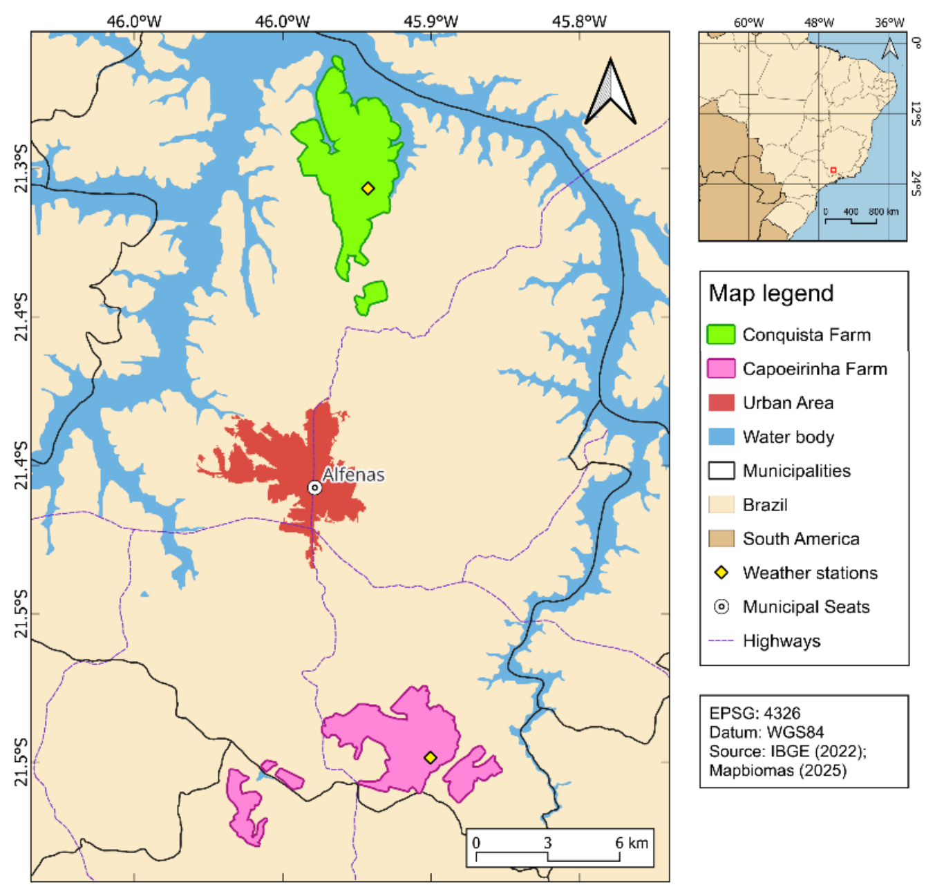
Figure 2.
Hierarchical workflow for the analysis of climate trends and correlations.
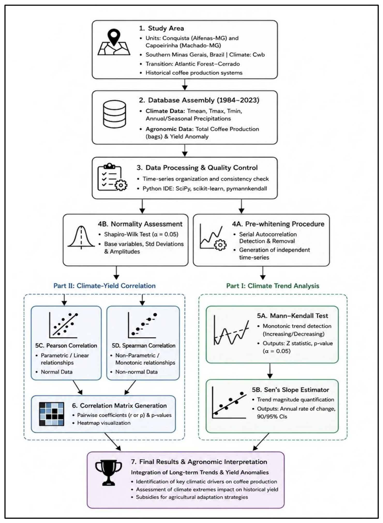
Figure 3.
Trend analysis of meteorological variables at the Capoeirinha production unit (1984–2023). (a) Maximum temperature in April; (b) Maximum temperature in September; (c) Mean temperature in April; (d) Mean temperature in May; (e) Mean temperature in September; (f) Minimum temperature in June; (g) Minimum temperature in September; (h) Minimum temperature in October; (i) Precipitation in May. Solid blue lines show the trends estimated using Sen’s slope.
Figure 3.
Trend analysis of meteorological variables at the Capoeirinha production unit (1984–2023). (a) Maximum temperature in April; (b) Maximum temperature in September; (c) Mean temperature in April; (d) Mean temperature in May; (e) Mean temperature in September; (f) Minimum temperature in June; (g) Minimum temperature in September; (h) Minimum temperature in October; (i) Precipitation in May. Solid blue lines show the trends estimated using Sen’s slope.
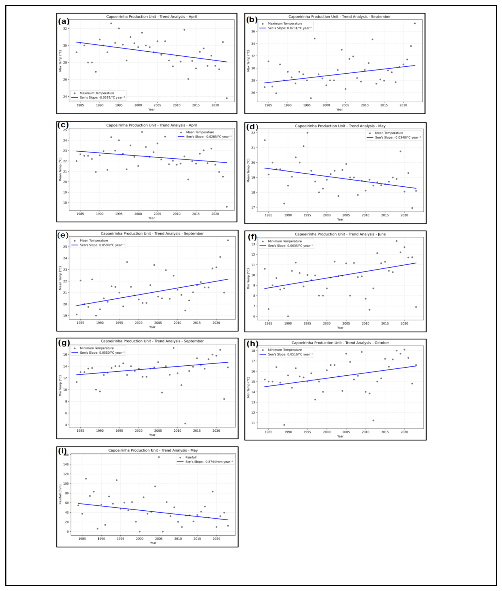
Figure 4.
Trend analysis of meteorological variables at the Conquista production unit (1984–2023). (a) Maximum temperature in April; (b) Maximum temperature in September; (c) Maximum temperature in December; (d) Mean temperature in April; (e) Mean temperature in May; (f) Mean temperature in December; (g) Minimum temperature in June; (h) Minimum temperature in September; (i) Cumulative dry-season precipitation. Solid blue lines show the trends estimated using Sen’s slope.
Figure 4.
Trend analysis of meteorological variables at the Conquista production unit (1984–2023). (a) Maximum temperature in April; (b) Maximum temperature in September; (c) Maximum temperature in December; (d) Mean temperature in April; (e) Mean temperature in May; (f) Mean temperature in December; (g) Minimum temperature in June; (h) Minimum temperature in September; (i) Cumulative dry-season precipitation. Solid blue lines show the trends estimated using Sen’s slope.
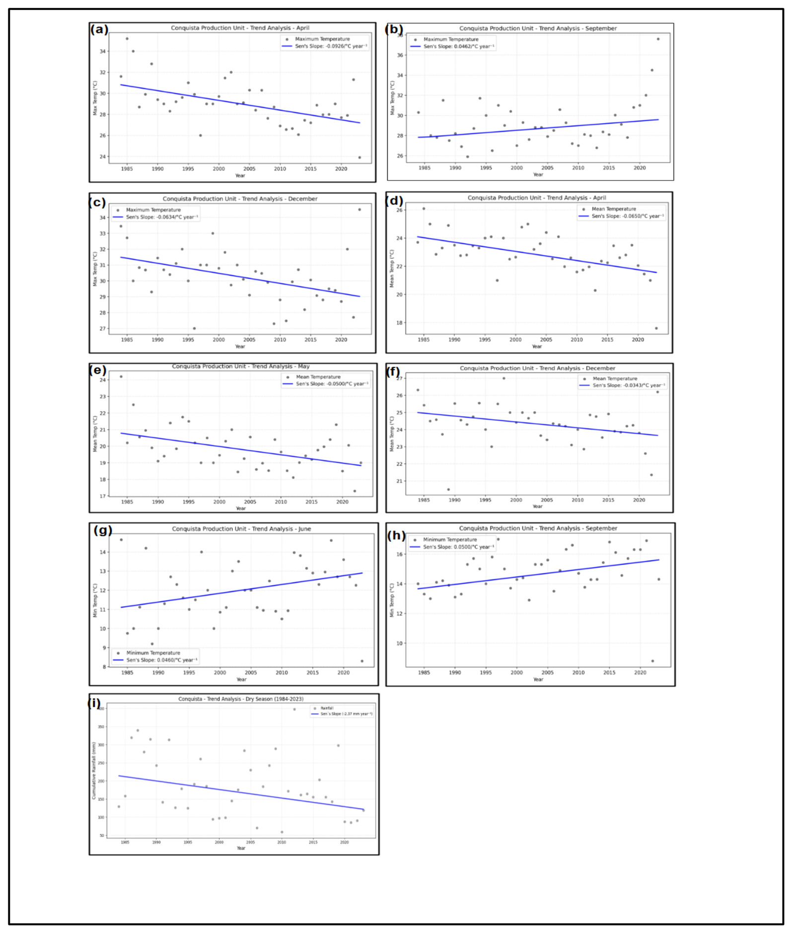
Figure 5.
Comparison of estimated changes between the production units. (a) Monthly magnitudes of change in maximum, mean, and minimum temperatures over the historical series; (b) Monthly precipitation changes; (c) Wet-season precipitation changes; (d) Dry-season precipitation changes. Filled black symbols indicate statistically significant trends (p < 0.05). Shaded areas indicate the direction of change: red denotes warming in (a) and drier conditions in (b-d), while blue denotes cooling in (a) and wetter conditions in (b-d). .
Figure 5.
Comparison of estimated changes between the production units. (a) Monthly magnitudes of change in maximum, mean, and minimum temperatures over the historical series; (b) Monthly precipitation changes; (c) Wet-season precipitation changes; (d) Dry-season precipitation changes. Filled black symbols indicate statistically significant trends (p < 0.05). Shaded areas indicate the direction of change: red denotes warming in (a) and drier conditions in (b-d), while blue denotes cooling in (a) and wetter conditions in (b-d). .
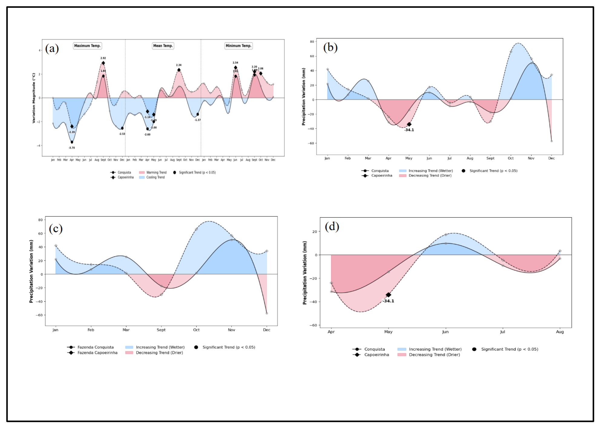
Figure 6.
Correlations between climatic and agronomic variables at the Capoeirinha production unit. (a) complete correlation matrix; (b) selected correlations of climatic variables with coffee yield; and (c) selected correlations of climatic variables with total production.
Figure 6.
Correlations between climatic and agronomic variables at the Capoeirinha production unit. (a) complete correlation matrix; (b) selected correlations of climatic variables with coffee yield; and (c) selected correlations of climatic variables with total production.
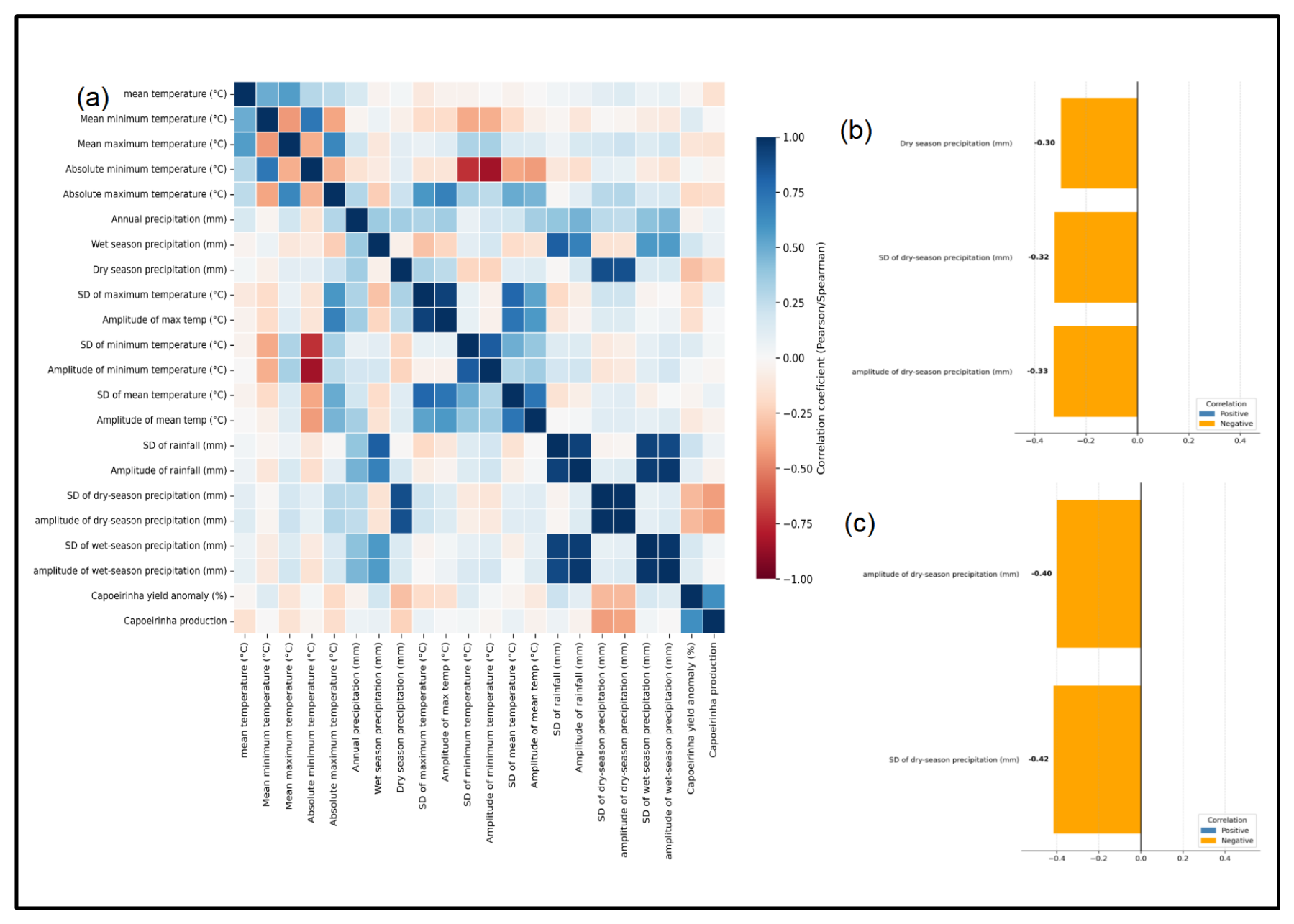
Figure 7.
Correlations between climatic and agronomic variables at the Conquista production unit. (a) complete correlation matrix; (b) selected correlations of climatic variables with coffee yield; and (c) selected correlations of climatic variables with total production.
Figure 7.
Correlations between climatic and agronomic variables at the Conquista production unit. (a) complete correlation matrix; (b) selected correlations of climatic variables with coffee yield; and (c) selected correlations of climatic variables with total production.
Disclaimer/Publisher’s Note: The statements, opinions and data contained in all publications are solely those of the individual author(s) and contributor(s) and not of MDPI and/or the editor(s). MDPI and/or the editor(s) disclaim responsibility for any injury to people or property resulting from any ideas, methods, instructions or products referred to in the content. |
© 2026 by the authors. Licensee MDPI, Basel, Switzerland. This article is an open access article distributed under the terms and conditions of the Creative Commons Attribution (CC BY) license (http://creativecommons.org/licenses/by/4.0/).
Copyright: This open access article is published under a Creative Commons CC BY 4.0 license, which permit the free download, distribution, and reuse, provided that the author and preprint are cited in any reuse.