

Submitted:
07 August 2026
Posted:
11 August 2026
You are already at the latest version
Abstract
Radar sensors, which enable the identification of the navigational situation and a preliminary assessment of collision risk, form the basis for safe ship control. This paper presents the author’s quantitative methods for assessing collision risk in the context of multi-ship navigation, and then synthesizes safe control methods. This study proposes four neural domain variants and three mathematical models of collision risk. Proprietary methods are presented: neural dynamic control (NDC) and game-based control (GC). An experimental comparison of these control methods is conducted using data from real-world navigation scenarios. Therefore, under favorable traffic conditions, the NDC method proves to be the most effective, while the GC method facilitates effective cooperative and non-cooperative management in situations of restricted ship traffic. The safe control methods proposed in this study will contribute to increased navigation safety, particularly in situations of high ship traffic density and challenging environmental conditions.
Keywords:
sensing in safety navigation development
; artificial intelligence
; safe control
; game control
; collision risk
1. Introduction
The most important task in ship design and construction is the development of algorithms and computer programs for their safe control [1]. For this purpose, the ship must be equipped with a computer system, measurement sensors, and navigation devices, from which the recorded parameters are processed and used to control the ship. The paper [2] concluded that existing marine mobility structures lack the necessary sensors to avoid emergency situations, such as floods, oil spills, or health hazards, which require effective monitoring. Sensor energy efficiency, data processing, sensor fusion methodologies, and accurate description of sea state with environmental monitoring using unmanned vehicles are crucial.
The sensing system proposed in [3] utilizes optical and radar data collected from satellite imagery sensors to investigate the activity patterns of maritime vessels. This system utilizes dedicated processing units to discover targets from images based on vessel type, classify those vessel classes according to their geometric and dispersion characteristics, evaluate their kinematics, assess their navigation behaviors, and predict their routes. In [4], multiple dimensions of sensing are examined using multispectral and multi-sensor technologies, and oceanic phenomena observed via multispectral and search and rescue (SAR) imagery concerning oceans, sea ice, and ship surveillance are analyzed for tracking and navigation needs. A comparative analysis of algorithms designed for collision avoidance and real-time ship routing using radar sensing to identify ship echoes has been presented in [5]. The development of an intelligent navigation system for vessels is grounded in risk assessment that includes collaboration between ships and shore facilities, as well as the evolving risks linked to smart ship navigation through various sensing methodologies, navigational situations, and event chain implications, as discussed in [6]. Sensing facilitates maritime surveillance by enabling the detection and identification of marine traffic from space, utilizing data sourced from satellites. The validation of vessel detections via space-based imagery can be supported by information gathered from the AIS, as noted in [7].
The concept of the ship domain is crucial in the context of intelligent collision avoidance systems and maritime traffic engineering; publication [8] presents traditional ship domain models while discussing their practical applications.
In [9], a methodology for identifying risks in ship navigation merges the concept of the ship domain with sensing data and AIS inputs to enhance prediction accuracy regarding collision risks in intricate waterways. The model of the ship domain is developed using a density map derived from AIS data. Furthermore, reference [10] presented a collision risk model that utilizes the ship domain alongside relevant parameters associated with collision risks, which analyzes encounters between ships through five variables: degree of domain infringement, relative speeds between vessels, course combinations, arena violations, and complexity during encounters. Traditional models assessing collision risk based on distance at closest point of approach (DCPA) or time to closest point of approach (TCPA) fall short in effectively estimating collisions or planning avoidance strategies. Therefore, an elliptical dynamic ship domain was designed in [11] to enable adaptation to varying speed and maneuverability features. Navigating potential collision hazards with vessels requires making judgments in an environment of uncertainty, especially when issues such as collision risk or safe speeds are considered. Using fuzzy logic, a novel artificial intelligence (AI) system was shown to be capable of finding safe routes for ships facing potential collisions in [12]. Ref. [13] detailed relevant development steps, such as analyzing the collision risk among ships, identifying crucial points in traffic, and determining how to plan a route correctly to avoid collisions. Based on [12], we present proposals for the identification of hazards in conjunction with ML algorithms for adverse weather. For collision risk assessment, documented incidents have been examined along with their environmental impacts, for which common analytical frameworks (e.g., probabilistic methods) have been used (for example, in [13]). Results from the research presented in [16] suggest that collision risk prediction can be performed based on DL models using long-term memory networks and Bayesian assessments. Using the hazard-exposure-sensitivity model, pixel-wise navigational risk maps were presented that visualize high-risk areas, mainly near major ports and their access channels; the highest exposure to navigational hazards is recorded for cargo ships, followed by tankers, tugboats, etc. [17]. In [18], a literature review focused on the identification of navigational threats for intelligent vessels was presented, which covered four domains; namely, environmental hazards, management practices, equipment reliability, and the effectiveness of navigation systems. Based on the maritime autonomous surface ships (MASS) operations data and research context, risk assessment methods relevant to MASS operations use a layered approach that combines failure mode analysis with Dempster–Shafer evidence theory and Bayesian networks, as described in [19]. Reference [20] also presented a model seeking to flexibly prioritize failure modes and improve safety controls through the functionalization of autonomous navigation systems. Another study used an approach that combines aspects of game theory, where ships at risk are presented as individual players who plan strategically and independently in a game context and use game rules [21]; when their vessel trajectories change, such decisions are framed as strategic decisions, including optimization and adherence to safety and socio-economic norms, as well as socio-economic constraints influencing ship actions.
In summary, the above references addressed separate types of sensing: ship motion, collision risk, and danger domains, and the less multi-ship and game nature of the safe steering process. This paper, rather than combining the above sensing tasks, leads to their use in the synthesis of adequate methods for safe ship control.
The aim of this work is to demonstrate that by measuring the process state using ARPA radar and then using selected artificial intelligence and game theory methods, it is possible to synthesize safe control methods in situations where many ships pass each other in different navigation conditions.
The main achievements of this work include:
- Synthesis of neural-dynamic and cooperative and non-cooperative game-based control methods for ensuring ship safety using sensing of collision risk;
- Assessment of the sensitivity of safe ship control to changes in visibility conditions at sea.
This paper is structured as follows: Chapter 2 first presents the task of safe ship control based on information from on-board sensors, and then the methods of synthesis of control methods and analysis of their sensitivity. Section 3 presents the results of simulation studies of the methods in three real-world navigation situations. Section 9 synthesizes the effectiveness of the new control methods presented in the paper. Conclusions are presented in Section 5.
2. Methodologies
In multi-vessel situations, utilizing information from onboard sensors and then combining appropriate safety control techniques based on artificial intelligence and game theory enables safe vessel control. This approach addresses previously overlooked factors affecting navigational safety and significantly reduces the likelihood of collisions.
In this section, two safe control methods based on artificial intelligence and game theory, developed by the author of this article, are presented.
2.1. Control Task
A functional diagram of the control process, extending from remote sensing to secure control implementation, is shown in Figure 1.
In multi-ship navigation situations, controlling the subject ship requires selecting the optimal trajectory among possible safe paths using artificial intelligence and game theory tools. This requires first formulating a mathematical model of the control process, then applying an appropriate optimization technique [22]. The effectiveness of optimization depends on how well the model reflects the actual kinematics and dynamics of the control process. In this study, navigational safety is quantified either by the size of the passing ship domains generated via a neural network, or by predicting the collision risk using an appropriate mathematical model. Both the kinematic and dynamic characteristics of the ships, as well as their degree of cooperation, are taken into account.
2.2. Neural-Dynamic Control
The mathematical description of the control process includes the kinematic and dynamic equations of the subject ship and the dynamic constraints assigned to each encountered ship j. The kinematics of the motion of the subject ship relative to other ships are schematically presented in Figure 2.
The dynamics of the subject ship as an astatic object controlling the change in its course y0, with time constant Ty and gain ky, are represented by the following nonlinear differential equation:
where α is the rudder angle, while (a1, a2) are the coefficients of the nonlinear static of the subject ship characteristic .
The speed control dynamics V0 for the subject ship are described via a second-order static inertial system with time constants Tv1 and Tv2 and a gain kv that reflects inertial effects during speed changes in anti-collision maneuvers, as follows:
where n0 represents the rotational speed of the ship’s own propulsion system.
The model of the entire process includes the dynamics of maneuvering the subject ship (changes in course y0 and speed V0) and the kinematics of the passing ships, which move at a constant course yjand constant speed Vj. The motion of the passing ships is taken into account in the constraints of the control process via mobile perilous domains generated using an artificial neural network.
In this way, the following state equations and constraints of the NDC model are obtained:
where, for the own ship state and the control variables: (x1, x2) = (x0, y0) are the position coordinates, x3 = y0 is the heading, x4 = is the angular velocity of the course change, x5 = V0 is the velocity, x6 = is the acceleration, u01 = a0 is the rudder deflection, and u02 = n0 is the propeller speed.
The transport process constraints C are defined as follows:
where jj and Dj denote the bearing to and distance from ship j, respectively, and Ts and Ds represent the safe time and distance for the subject ship relative to the approaching ship j.
To implement constraint (4) of the control process—namely, the safe passing of the subject ship by ship j—an artificial neural network was used to estimate the collision risk rj, and the size of the dangerous maneuver domains assigned to the encountered ships was adjusted. Examples of the domain shapes are illustrated in the form of a hexagon in Figure 3.
To reflect the navigator’s subjective maneuvering decisions, the domain sizes change over the course of the ship j’s motion process proportional to the collision risk. The neural network, implemented in the MATLAB 2026 Neural Network Toolbox, consists of three neural layers with nonlinear activation functions in the first two layers and a sigmoidal output activation in the third. Backpropagation with an adaptive, adjusted learning rate and momentum based on the expert navigator’s data were used to train the network.
The domain dimensions are scaled according to the network output, which represents the collision risk; these domains are assigned to individual passing ships and move at their speeds in the dynamic programming plane [23,24].
Among the real-time dynamic optimization techniques, dynamic programming proved to be the most suitable option for modeling the considered control process defined by the state (3) and time-dependent state constraints (4). Since collision avoidance satisfied the duality conditions, the time-optimal path of the subject ship was derived based on Bellman’s principle, proceeding from stage k = 1 to stage K. The state equations in discrete form are defined as follows:
According to Bellman’s principle, the time-optimal control of the subject ship at stage k of the trajectory is given by the following formula:
The NDC method uses the state description of the control process (5) to model the dynamic motion of the subject ship, and (6) determines its time-optimal control, taking into account the kinematics of the passing ships, represented by their neural domains.
According to the Nyquist–Shannon sampling theorem, the discrete time step Dtk in Equation (6) was set as approximately an order of magnitude smaller than the time constant Tψ of the subject ship 0 (i.e., from 1 s to 30 s), depending on the ship’s tonnage. The state-space grid resolution depends on the duration of the subject ship’s course-change maneuvers, which, according to control theory, is approximately three time constants Tψ, and then converted to navigational distance. Consequently, the dynamic programming grid resolution ranges from 0.1 nautical miles to 1.0 nautical mile.
2.3. Game Control
A multi-stage matrix game was constructed as a matrix R containing collision risk values rj for permissible course or speed changes for the subject ship (rows) as n strategies s0,n and other ships (j) (columns) as m strategies sj,m:
where n = 1, 2, ..., N denotes the number of strategies for the subject ship, and m = 1, 2, ..., M denotes strategies for the other ships.
Many mathematical formulas are available for estimating collision risk [26,27,28,29,30]. Ship collision risk models include both probabilistic, physics-based methods and advanced machine learning algorithms that consider ship attributes, as well as navigational and environmental factors. The presented models quantify the risk of collision rj using parameters such as DCPA = and TCPA = .
In this article, the author proposes the following formulas: logarithmic (log), mean square (ms), and hyperbolic (hyp).
The logarithmic model log calculates the risk of collision rj between the subject ship and ship j using a logarithmic function that emphasizes the distance between ships Dj, especially in situations of excessive proximity:
where denote the distance and time to closest approach between the subject ship and the encountered ship j, while Ds and Ts are predetermined safe distance and approach time values for the subject ship and ship j in the actual navigational situation.
In the root-mean-square model ms, risk of collision rj is represented as the reciprocal of the square root of the average of the squares of the individual quantities and time to closest approach and relative proximity :
In the hyperbolic model hyp, collision risk rj with ship j is inversely proportional to the relative distance and time values:
The collision risk graphs presented in Figure 4 for individual models were created in Matlab 2026 software [31].
As the assumed matrix game does not have a saddle point in real navigational situations, its solution is carried out in mixed strategies, expressed as probability distributions of the pure strategies of the subject ship and the J passed ships. To aggregate the strategies of the subject ship over all J ships, the entropy H was used to assess the certainty of the components of the pure strategies:
The mixed-strategy Nash equilibrium acts as a minimax solution, meaning that the expected payoff in the equilibrium guarantees each player the optimal outcome against the most hostile, rational opponent [34,35].
The GCc cooperative game control method is based on dual linear programming. Finding the optimal strategy for the subject ship , with strategy probabilities , minimizes the risk of collision with ship j,
with the conditions
and the cooperating ship encountered also minimizes the risk of collision:
In the GCnc non-cooperative control method, the encountered ship j maximizes the risk of collision with the subject ship,
with the conditions
In summary, the GC game control method uses the state equations of ship motion kinematics; the optimal strategy for the subject ship (12) and the two-criteria game optimization involves using either Formulas (13) and (16) or Formulas (13) and (17).
2.4. Sensitivity of Safe Control
The sensitivity of NDC, of GC and of NGC are defined as the relation of the relative change in the final deviation d in the subject ship’s safe trajectory to the relative change in the safe passing distance Ds:
The sensitivity srj of collision risk is defined as the relationship between the changes in the risk of collision and the relative changes in the distance and time to excessive approach of the ships:
For the logarithmic model log, the collision risk sensitivity is
For the mean-square model ms, the collision risk sensitivity is
For the hyperbolic model hyp, the collision risk sensitivity is
The sensitivity characteristics of collision risk according to relative changes in safe distance and approach time for the log, ms, and hyp models are presented in Figure 5.
From these sensitivity plots, it can be seen that when distances and times approach their safe thresholds, the hyperbolic model hyp exhibits the greatest sensitivity in tight-proximity scenarios, while the logarithmic model log shows the least sensitivity.
3. Experimental Results
A comparative evaluation of the NDC and GC methods for safe control of the subject ship was conducted in situations with varying numbers of passing ships. The simulation studies were based on actual navigational situations recorded on the research and training vessel r/v HORYZONT II: L = 56.34 m; B = 11.36 m; T = 5.3 m; DWT = 396 t [36]. The navigational situations were recorded on the SAM Electronics ARPA radar in the Skagerrak and Kattegat Straits in September 2025 during a training and research cruise to Spitsbergen (Figure 6).
Simulation tests were performed on navigational situations involving the subject ship passing J = 1, 3, and 12 ships, whose motion parameters are presented in Table 1.
Figure 7 visualizes the studied navigational situations in the form of ship velocity vectors.
3.1. Computer Simulation of the NDC Algorithm
Figure 8, Figure 9 and Figure 10 show the results of computer simulations of the safe trajectories of the subject ship when passing 1, 3, and 12 other ships, conducted under conditions of good visibility at sea at Ds = 1 nm and restricted visibility at Ds = 3 nm; the NDC method establishes constraints on the process state, represented by a hexagon NDC_h, a parabola NDC_p, and an ellipse NDC_e.
The secure and ideal course is influenced by the existing navigation circumstances. As stipulated by the COLREGs, this is assessed through the safe passing distance Ds, which varies from about 0.5 nautical miles in clear visibility to 3.0 nautical miles in severely limited visibility at sea. The characteristics of the final deviation d in the safe subject ship’s trajectory, determined by the NDC method, depending on the safe passing distance Ds, were compared with the characteristics calculated using the non-game control method (NGC), previously developed by the author (Figure 11).
The neural-dynamic control method NDC_h with hexagonal domains when passing J ships exhibits the largest final deviation d in the subject ship’s safe trajectory, and the smallest with ellipsoidal domains. This deviation, compared to the NGC method, is larger for a small number of passing ships and comparable for a larger number of passing ships.
Figure 12 illustrates the sensitivity attributes of a ship safe control in response to variations in navigation conditions. These characteristics are derived from the neural-dynamic control method utilizing ship domains represented as hexagons NDC_h, parabolas NDC_p, and ellipses NDC_e and, for comparison, performing assessment according to the non-game control NGC method. The sensitivity values of safe control were calculated via Equation (20) for the graphs shown in Figure 11.
The neural-dynamic control method with hexagonal domains NDC_h for J passing ships shows the highest sensitivity, and that with ellipsoidal domains NDC_e shows the lowest sensitivity. However, the sensitivity is comparable for small safe distance values Ds regardless of the number of passing ships.
3.2. Computer Simulation of the GC Algorithm
The GC field control method presented in Section 2.3 enabled simulation experiments to be conducted in conditions of cooperation and non-cooperation between the subject ship and ships j to avoid collisions. Figure 13 presents the ship trajectories determined via the cooperative field control method GCc_log and the non-cooperative field control method GCnc_log with a logarithmic collision risk rj model in a situation in which the subject ship passed J = 3 ships.
Figure 14, Figure 15 and Figure 16 show the simulation results for the subject ship safe trajectories in situations in which it passed J = 1, 3, and 12 ships, both in conditions of good visibility at Ds = 1 nm and restricted visibility at Ds = 3 nm, determined via the cooperative and non-cooperative GC methods, taking into account three collision risk models rj: logarithmic log, mean square ms, and hyperbolic hyp.
The GC_log control method with a logarithmic collision risk model shows the smallest final deviation d in the subject ship’s safe trajectory from the reference route, while the GC_hyp method with a hyperbolic model shows the largest final deviation. Tripling the safe passing distance Ds due to restricted visibility at sea doubles the deviation in the subject ship’s trajectory from the predetermined route. The GCnc method, on the other hand, increases the deviation d in the trajectory compared to the GCc algorithm by 30–50%.
The quality of the safe game control is characterized by the value d of the final deviation in the subject ship’s safe trajectory from the reference voyage route, depending on the navigational situation, related to the value of the safe passing distance Ds resulting from the COLREG requirements. Figure 17 shows a comparison of the deviation characteristics for game control and non-game control.
Figure 18 shows the sensitivity characteristics of the safe control of the subject ship to changes in navigation conditions, corresponding to the following collision risk models: logarithmic GC_log, mean square GC_ms, and hyperbolic GC_hyp. The sensitivity values for safe control were calculated using Equation (25) for the graphs shown in Figure 17.
4. Discussion
To assess the effectiveness of safe ship control using the NDC and GC methods, the relative sensitivity metric can be defined as
where the values of and are obtained from Formula (20) [37,38].
The characteristics of the effectiveness of the safe control of the subject ship s0, based on the simulation results of the methods that form the bases of Figure 12 and Figure 18, are presented in Figure 19.
In good visibility conditions at sea and with lower required safe passing distances Ds, the GCnc method is most effective at 80%. As navigational conditions deteriorate and Ds values need to be increased, the GCc method is most effective at 60%, followed by the NDC method at a lesser extent (35%).
Despite these favorable findings, this study has several limitations. The NDC method is extremely sensitive to the shape of the passing ship domains, and the GC method is highly dependent on the form of the mathematical collision risk model.
5. Conclusions
Simulation studies demonstrated the correct operation of safe ship control algorithms in complex multi-ship traffic situations by taking into account environmental visibility constraints and the level of cooperation between ships resulting from the interpretation of COLREG traffic priority rules. The effectiveness of the NDC method, which utilizes artificial intelligence elements in the form of an artificial neural network that assigns collision risk domains to ships, was compared with the effectiveness of the GC method, which utilizes game-theoretic elements that consider ship cooperation—or lack thereof—in avoiding collisions.
Compared to previous studies, the novelty of this study is the joint application of neural network methods and game control under realistic navigation scenarios, with both good and restricted visibility at sea [5,8,10,21,23,30].
The methodology used in this study shows how AI and game theory can tackle the following practical aspects of safe navigation:
- Safe passing in multi-ship traffic situations;
- The coordination of ships to ensure collision avoidance;
- The impact of the current navigational situation on navigational safety.
As the NDC and GC methods enable live generation of neural domains and ship equilibrium states in risk games, they provide more realistic representations of control mechanisms, making them a promising approach for improving maritime safety.
In the future, it is necessary to investigate the sensitivity of safe ship control methods to inaccuracies of sensors of the current navigational situation and develop a method for visualizing safe ship trajectories in real time.
Funding
This research was funded as part of the research project of the Faculty of Computer Science, Gdynia Maritime University, Poland, No. WI/2026/PZ/02: “Development of methods and algorithms for environmental perception, navigation and control of autonomous vehicles”.
Data Availability Statement
All data supporting the findings of this study are available within the article.
Conflicts of Interest
The author declare no conflicts of interest.
References
- Szelangiewicz, T.; Zelazny, K.; Antosik, A.; Szelangiewicz, M. Application of Measurement Sensors and Navigation Devices in Experimental Research of the Computer System for the Control of an Unmanned Ship Model. Sensors 2021, 21, 1312. [Google Scholar] [CrossRef] [PubMed]
- Briguglio, G.; Crupi, V. Review on Sensors for Sustainable and Safe Maritime Mobility. J. Mar. Sci. Eng. 2024, 12, 353. [Google Scholar] [CrossRef]
- Reggiannini, M.; Salerno, E.; Bacciu, C.; D’Errico, A.; Lo Duca, A.; Marchetti, A.; Martinelli, M.; Mercurio, C.; Mistretta, A.; Righi, M.; et al. Remote Sensing for Maritime Traffic Understanding. Remote Sens. 2024, 16, 557. [Google Scholar] [CrossRef]
- Heiselberg, H.; Stateczny, A. Remote Sensing in Vessel Detection and Navigation. Sensors 2020, 15, 5841. [Google Scholar] [CrossRef] [PubMed]
- Lazarowska, A. Review of Collision Avoidance and Path Planning Methods for Ships Utilizing Radar Remote Sensing. Remote Sens. 2021, 13, 3265. [Google Scholar] [CrossRef]
- Luo, J.; Geng, X.; Li, Y.; Yu, Q. Study on the Risk Model of the Intelligent Ship Navigation. Wirel. Commun. Mob. Comput. 2022, 2022, 3437255. [Google Scholar] [CrossRef]
- Melillos, G.; Themistocleous, K.; Danezis, C.; Michaelides, S.; Hadjimitsis, D.G.; Jacobsen, S.; Tings, B. The use of remote sensing for maritime surveillance for security and safety in Cyprus. In Proceedings of the SPIE 11418, Detection and Sensing of Mines, Explosive Objects, and Obscured Targets XXV; SPIE: Bellingham, WA, USA, 2020. [Google Scholar] [CrossRef]
- Li, W.; Cheng, K.; Shi, G.; Desrosiers, R.; Wang, X. Ship domain models: Reviewing the advancements and exploring the future directions in the maritime autonomous surface ships. Ocean Eng. 2025, 326, 120935. [Google Scholar] [CrossRef]
- Wang, Z.; Wu, Y.; Chu, X.; Liu, C.; Zheng, M. Risk Identification Method for Ship Navigation in the Complex Waterways via Consideration of Ship Domain. J. Mar. Sci. Eng. 2023, 11, 2265. [Google Scholar] [CrossRef]
- Szlapczynski, R.; Szlapczynska, J. A ship domain-based model of collision risk for near-miss detection and Collision Alert Systems. Reliab. Eng. Syst. Saf. 2021, 214, 107766. [Google Scholar] [CrossRef]
- Li, W.; Zhong, L.; Xu, Y.; Shi, G. Collision Risk Index Calculation Based on an Improved Ship Domain Model. J. Mar. Sci. Eng. 2022, 10, 2016. [Google Scholar] [CrossRef]
- Mohamed-Seghir, M. Decision support system using modern methods of collision avoidance in collision situations at sea. TransNav Int. J. Mar. Navig. Saf. Sea Transp. 2026, 20, 55–60. [Google Scholar] [CrossRef]
- Yu, H.; Meng, Q.; Fang, Z.; Liu, J.; Xu, L. A review of ship collision risk assessment, hotspot detection and path planning for maritime traffic control in restricted waters. J. Navig. 2022, 75, 1337–1363. [Google Scholar] [CrossRef]
- Wu, Z.; Wang, S.; Li, L.; Wang, Y.; Wang, X. Ship near-miss risk identification method based on mult-model deep fusion model under complex weather and sea conditions. Ocean Eng. 2025, 329, 121119. [Google Scholar] [CrossRef]
- Firdaus, M.I.; Zaman, M.B.; Gurning, R.O.S. A Comprehensive Review of Ship Collision Risk Assessment and Safety Index Development. Safety 2026, 12, 57. [Google Scholar] [CrossRef]
- Zhou, F.; Wang, S. A Hybrid Framework Integrating End-to-End Deep Learning with Bayesian Inference for Maritime Navigation Risk Prediction. J. Mar. Sci. Eng. 2025, 13, 1925. [Google Scholar] [CrossRef]
- Lin, Z.; Yan, Y.; Hou, Q.; Gao, J.; Xu, Y. Remote sensing and AIS-based navigation risk assessment under sea ice conditions in the Bohai Sea. Ocean Coast. Manag. 2026, 273, 108029. [Google Scholar] [CrossRef]
- Hanhua, X.; Ke, Z. A Review and Prospects of Navigation Risk Assessment Methods for Intelligent Ships. In Proceedings of the 2025 International Conference on Artificial Intelligence and Autonomous Transportation AIAT; Lecture Notes in Electrical Engineering; Wang, S.F., Li, Z., Pei, M., Zhang, W., Tang, T., Rong, Y., Eds.; Springer: Singapore, 2026; Volume 1595. [Google Scholar] [CrossRef]
- Tekeli, M.M.; Akyuz, E.; Teixeira, Â.P. A multi-method approach to navigational risk assessment for maritime autonomous surface ships. Aust. J. Marit. Ocean Aff. 2025, 1–30. [Google Scholar] [CrossRef]
- Carpitella, S.; Certa, A.; Muriana, C. Risk Assessment Framework for Autonomous Ship Navigation Systems. In Proceedings of the 29th ISSAT International Conference on Reliability and Quality in Design, RQD2024-54, Miami, FL, USA, 8–10 August 2024. [Google Scholar]
- Cui, H.; Zhang, X.; Wang, J.; Wang, C.; Zheng, K. Dynamic game collision avoidance decision-making for autonomous and manned ships. Chin. J. Ship Res. 2024, 19, 238–247. [Google Scholar] [CrossRef]
- Hoang, K.D.; Fioretto, F.; Hou, P.; Yeoh, W.; Yokoo, M.; Zivan, R. Proactive dynamic distributed constraint optimization problems. J. Artif. Intell. Res. 2022, 74, 179–225. [Google Scholar] [CrossRef]
- Geng, X.; Wang, Y.; Wang, P.; Zhang, B. Motion plan of maritime autonomous surface ships by dynamic programming for collision avoidance and speed optimization. Sensors 2019, 19, 434. [Google Scholar] [CrossRef] [PubMed]
- Zaccone, R. A dynamic programming approach to the collision avoidance of autonomous ships. Mathematics 2024, 12, 1546. [Google Scholar] [CrossRef]
- Tennenholtz, M. Game theory and artificial intelligence. In Foundations and Applications of Multi-Agent Systems; D’Inverno, M., Luck, M., Fisher, M., Preist, C., Eds.; Springer: Berlin/Heidelberg, Germany, 2002; pp. 49–58. [Google Scholar]
- Naumov, P.; Yuan, Y. Intelligence in strategic games. J. Artif. Intell. Res. 2021, 71, 521–556. [Google Scholar] [CrossRef]
- Birmpas, G.; Gan, J.; Hollender, A.; Marmolejo-Cossío, F.J.; Rajgopal, N.; Voudouris, A.A. Optimally deceiving a learning leader in stackelberg games. In Proceedings of the 34th Conference on Neural Information Processing Systems NeurIPS 2020, Vancouver, BC, Canada, 6–12 December 2021; pp. 20624–20635. [Google Scholar]
- Guo, J.; Ji, Z.; Liu, Y. Controllability of game-based multi-agent system. Sci. China Inf. Sci. 2023, 66, 222206. [Google Scholar] [CrossRef]
- Wang, L.; Fu, F.; Chen, X. Mathematics of multi-agent learning systems at the interface of game theory and artificial intelligence. Sci. China Inf. Sci. 2024, 67, 166201. [Google Scholar] [CrossRef]
- Zaman, M.A.U.; Lauriere, M.; Koppel, A.; Başar, T. Robust cooperative multi-agent reinforcement learning: A mean-field type game perspective. In Proceedings of the 6th Annual Learning for Dynamics & Control Conference, Oxford, UK, 15–17 July 2024; pp. 770–783. [Google Scholar]
- Graphs in Matlab. Available online: https://se.mathworks.com/help/matlab/ref/plot.html (accessed on 20 July 2026).
- Leoneti, A.B.; Prataviera, G.A. Entropy-norm space for geometric selection of strict Nash equilibria in n-person games. Phys. A Stat. Mech. Appl. 2020, 546, 124407. [Google Scholar] [CrossRef]
- Choi, M.C.; Wolfer, G. Markov chain entropy games and the geometry of their Nash equilibria. ALEA Lat. Am. J. Probab. Math. Stat. 2025, 22, 925–952. [Google Scholar] [CrossRef]
- Alvim, M.S.; Chatzikokolakis, K.; Kawamoto, Y.; Palamidessi, C. Leakage and Protocol Composition in a Game-Theoretic Perspective. In Principles of Security and Trust. POST 2018; Lecture Notes in Computer Science; Bauer, L., Küsters, R., Eds.; Springer: Cham, Switzerland, 2018; p. 10804. [Google Scholar] [CrossRef]
- Zou, C.; Chen, L.; Fan, H.; Tian, X.; Liu, L.; Yang, Z. Enhancing maritime autonomous surface ship navigation safety: A dynamic risk assessment framework integrating system theoretic process analysis and stochastic Petri nets. Reliab. Eng. Syst. Saf. 2027, 277, 113125. [Google Scholar] [CrossRef]
- Research vessel HORYZONT II. Available online: https://www.vesselfinder.com/vessels/details/9231925 (accessed on 19 July 2026).
- Nise, N.S. Control Systems Engineering, 8th edition; California State Polytechnic University, John Wiley & Sons Inc., USA, 2019; ISBN 978-1-119-47422-7. [Google Scholar]
- Rosenwasser, E.; Yusupov, R. Sensitivity of Automatic Control Systems; CRC Press: Boca Raton, FL, USA, 2000; ISBN 978-0-849-3229293-8. [Google Scholar]
Figure 1.
A flow chart showing safe ship control in multi-ship situations, illustrated in the form of their six-minute velocity vectors. RADAR = radio detection and ranging; ARPA = automatic radar plotting aid; GYRO = gyrocompass; LOG = speed measurement; NDC = neural-dynamic control; GC = game control.
Figure 1.
A flow chart showing safe ship control in multi-ship situations, illustrated in the form of their six-minute velocity vectors. RADAR = radio detection and ranging; ARPA = automatic radar plotting aid; GYRO = gyrocompass; LOG = speed measurement; NDC = neural-dynamic control; GC = game control.
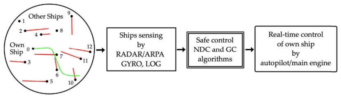
Figure 2.
Illustration of a control task demonstrating the safe and optimal trajectory of the subject ship and the relative motion of ship j in relation to the subject ship in an (X, Y) coordinate system. (y0, V0) represents the course and speed of the subject ship; (yj, Vj) represents the course and speed of ship j; (jj, Dj) represents the bearing of and distance to ship j.
Figure 2.
Illustration of a control task demonstrating the safe and optimal trajectory of the subject ship and the relative motion of ship j in relation to the subject ship in an (X, Y) coordinate system. (y0, V0) represents the course and speed of the subject ship; (yj, Vj) represents the course and speed of ship j; (jj, Dj) represents the bearing of and distance to ship j.
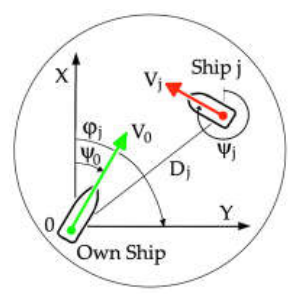
Figure 3.
Generating constraints that depict the collision risk rj through a neural network.
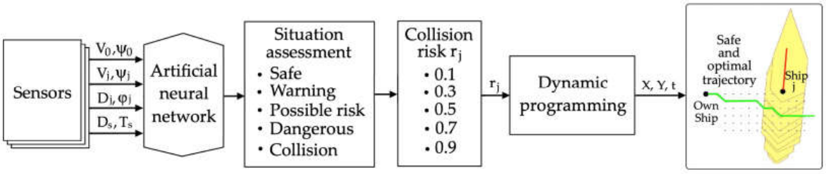
Figure 4.
Dependence of collision risk rj on relative values of distance and approach time of the subject ship and ship j for the three models: logarithmic log (left); mean square ms (middle); hyperbolic hyp (right).
Figure 4.
Dependence of collision risk rj on relative values of distance and approach time of the subject ship and ship j for the three models: logarithmic log (left); mean square ms (middle); hyperbolic hyp (right).
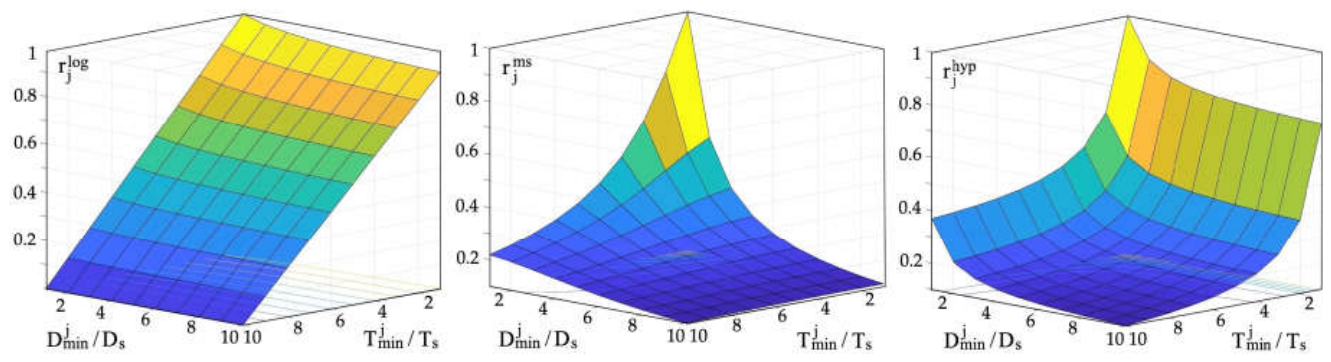
Figure 5.
Sensitivity characteristics srj of collision risk based on relative values of distance and approach time of the subject ship and ship j for the following models: logarithmic log (left); mean square ms (middle); hyperbolic hyp (right).
Figure 5.
Sensitivity characteristics srj of collision risk based on relative values of distance and approach time of the subject ship and ship j for the following models: logarithmic log (left); mean square ms (middle); hyperbolic hyp (right).
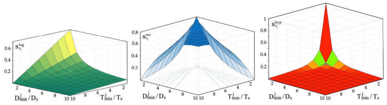
Figure 6.
Graphical presentation of the experimental case used to record navigational situations in the Skagerrak and Kattegat Straits on the research and training ship r/v HORYZONT II.
Figure 6.
Graphical presentation of the experimental case used to record navigational situations in the Skagerrak and Kattegat Straits on the research and training ship r/v HORYZONT II.
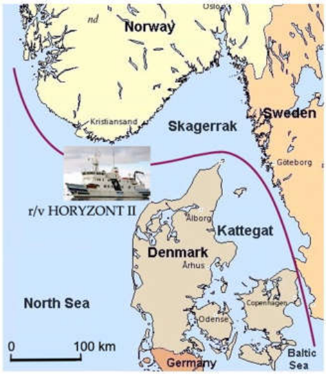
Figure 7.
The navigational situations of the subject ship’s motion when passing J ships, illustrated in the form of their six-minute velocity vectors: (a) J = 1; (b) J = 3; (c) J = 12.
Figure 7.
The navigational situations of the subject ship’s motion when passing J ships, illustrated in the form of their six-minute velocity vectors: (a) J = 1; (b) J = 3; (c) J = 12.
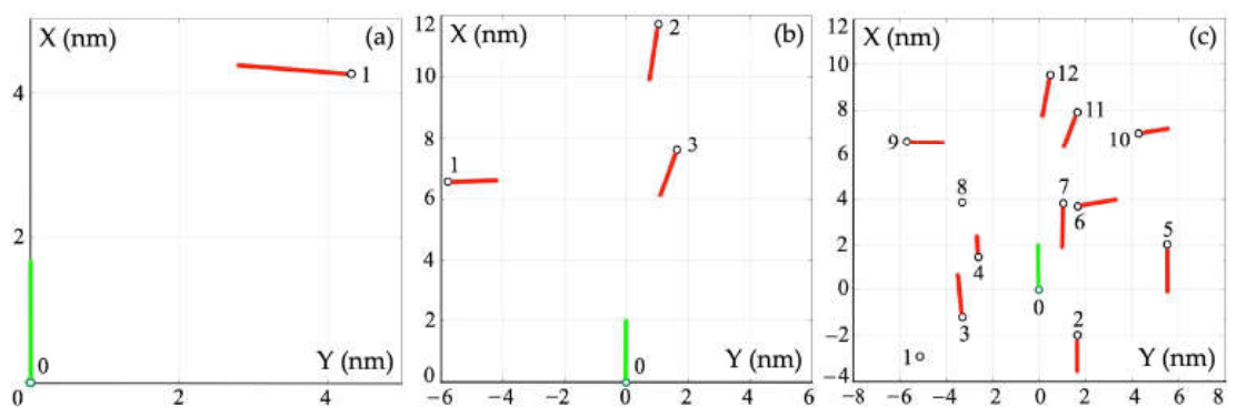
Figure 8.
Safe trajectories of the subject ship passing one ship (j = 1) under conditions of good visibility at Ds = 1 nm and restricted visibility at Ds = 3 nm, determined via the NDC method: (a) NDC_h with a hexagonal domain (red); (b) NDC_p with a parabolic domain (blue); (c) NDC_e with an elliptical domain (green).
Figure 8.
Safe trajectories of the subject ship passing one ship (j = 1) under conditions of good visibility at Ds = 1 nm and restricted visibility at Ds = 3 nm, determined via the NDC method: (a) NDC_h with a hexagonal domain (red); (b) NDC_p with a parabolic domain (blue); (c) NDC_e with an elliptical domain (green).
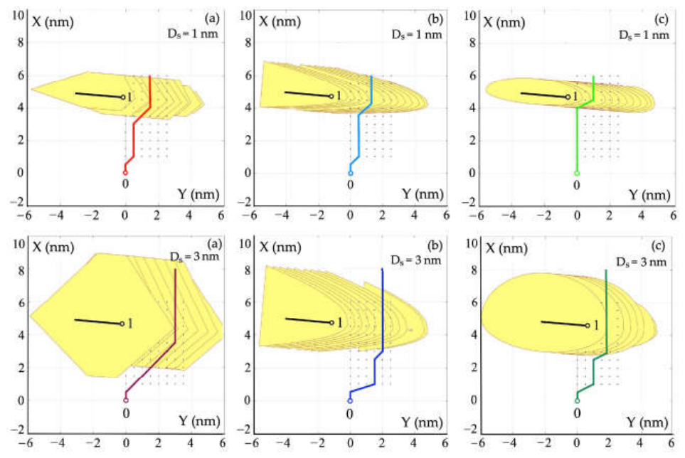
Figure 9.
Safe trajectories of the subject ship passing three ships (j = 3) under conditions of good visibility at Ds = 1 nm and restricted visibility at Ds = 3 nm, determined via the NDC method: (a) NDC_h with a hexagonal domain (red); (b) NDC_p with a parabolic domain (blue); (c) NDC_e with an elliptical domain (green).
Figure 9.
Safe trajectories of the subject ship passing three ships (j = 3) under conditions of good visibility at Ds = 1 nm and restricted visibility at Ds = 3 nm, determined via the NDC method: (a) NDC_h with a hexagonal domain (red); (b) NDC_p with a parabolic domain (blue); (c) NDC_e with an elliptical domain (green).
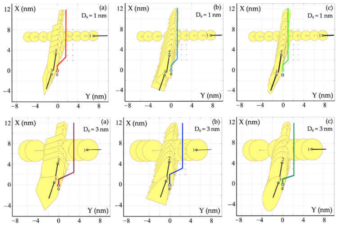
Figure 10.
Safe trajectories of the subject ship passing twelve ships (J = 12) under conditions of good visibility at Ds = 1 nm and restricted visibility at Ds = 3 nm, determined via the NDC method: (a) NDC_h with a hexagonal domain (red) (b) NDC_p with a parabolic domain (blue); (c) NDC_e with an elliptical domain (green).
Figure 10.
Safe trajectories of the subject ship passing twelve ships (J = 12) under conditions of good visibility at Ds = 1 nm and restricted visibility at Ds = 3 nm, determined via the NDC method: (a) NDC_h with a hexagonal domain (red) (b) NDC_p with a parabolic domain (blue); (c) NDC_e with an elliptical domain (green).
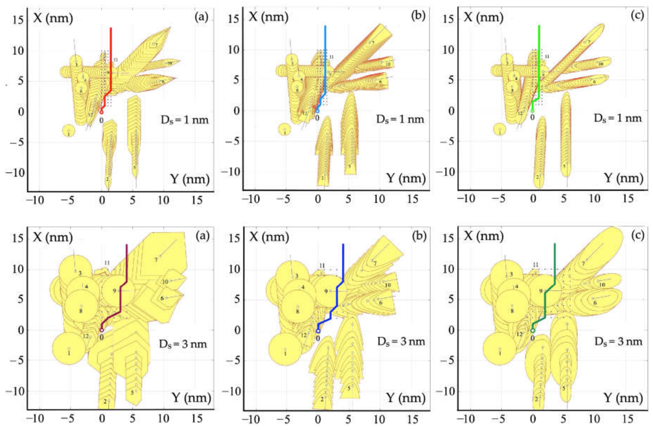
Figure 11.
Characteristics of the final deviation d in the subject ship’s safe trajectory determined according to the NDC_h, NDC_p, NDC_e, and NGC methods: (a) J = 1; (b) J = 3; (c) J = 12.
Figure 11.
Characteristics of the final deviation d in the subject ship’s safe trajectory determined according to the NDC_h, NDC_p, NDC_e, and NGC methods: (a) J = 1; (b) J = 3; (c) J = 12.
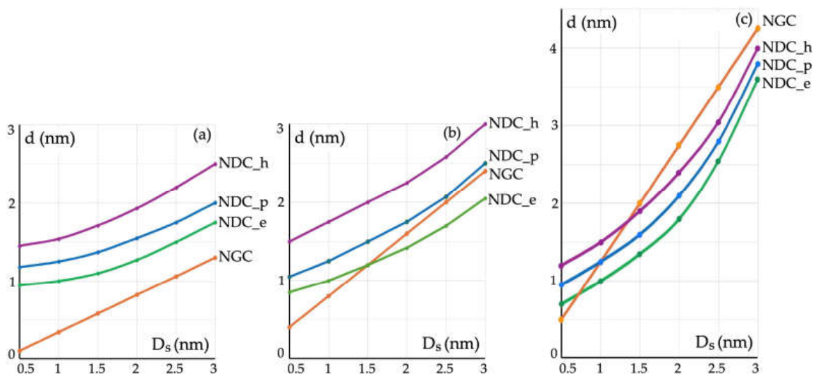
Figure 12.
Sensitivity characteristics of the final deviation d in the subject ship’s safe trajectory to changes in the safe distance Ds of the passing J ships: (a) J = 1; (b) J = 3; (c) J = 12.
Figure 12.
Sensitivity characteristics of the final deviation d in the subject ship’s safe trajectory to changes in the safe distance Ds of the passing J ships: (a) J = 1; (b) J = 3; (c) J = 12.
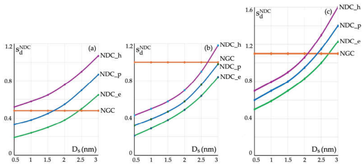
Figure 13.
Comparison of safe ship trajectories for cooperative (left) and non-cooperative (right) collision avoidance maneuvers, determined via the GCc_log and GCnc_log game control methods, respectively; and, for comparison, via the NGC non-game control method.
Figure 13.
Comparison of safe ship trajectories for cooperative (left) and non-cooperative (right) collision avoidance maneuvers, determined via the GCc_log and GCnc_log game control methods, respectively; and, for comparison, via the NGC non-game control method.
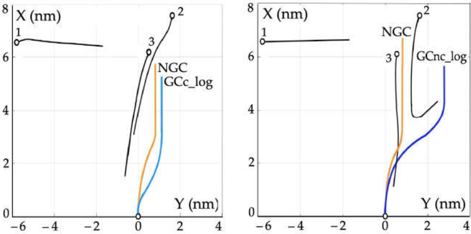
Figure 14.
Safe trajectories of the subject ship when passing one ship (J = 1) under conditions of good visibility at Ds = 1 nm (left) and restricted visibility at Ds = 3 nm (right), calculated using the cooperative and non-cooperative game control method with the collision risk model rj-logarithmic GCc_log and GCnc_log, mean square GCc_ms and GCnc_ms, and hyperbolic GCc_hyp and GCnc_hyp; for comparison, the trajectories of the non-game control NGC are presented.
Figure 14.
Safe trajectories of the subject ship when passing one ship (J = 1) under conditions of good visibility at Ds = 1 nm (left) and restricted visibility at Ds = 3 nm (right), calculated using the cooperative and non-cooperative game control method with the collision risk model rj-logarithmic GCc_log and GCnc_log, mean square GCc_ms and GCnc_ms, and hyperbolic GCc_hyp and GCnc_hyp; for comparison, the trajectories of the non-game control NGC are presented.
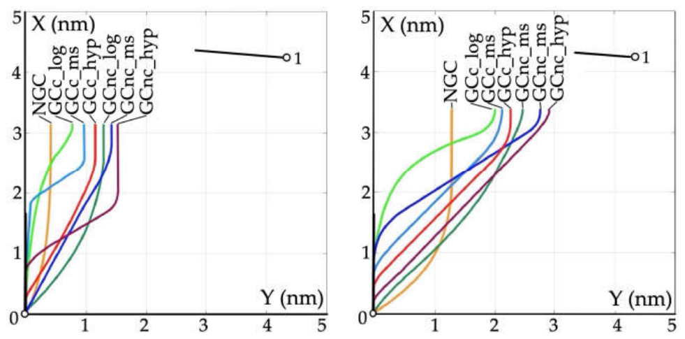
Figure 15.
Safe trajectories of the subject ship when passing one ship (J = 3) under conditions of good visibility at Ds = 1 nm (left) and restricted visibility at Ds = 3 nm (right), calculated using the cooperative and non-cooperative game control method with the collision risk model rj-logarithmic GCc_log and GCnc_log, mean square GCc_ms and GCnc_ms, and hyperbolic GCc_hyp and GCnc_hyp; for comparison, the trajectories of the non-game control NGC are presented.
Figure 15.
Safe trajectories of the subject ship when passing one ship (J = 3) under conditions of good visibility at Ds = 1 nm (left) and restricted visibility at Ds = 3 nm (right), calculated using the cooperative and non-cooperative game control method with the collision risk model rj-logarithmic GCc_log and GCnc_log, mean square GCc_ms and GCnc_ms, and hyperbolic GCc_hyp and GCnc_hyp; for comparison, the trajectories of the non-game control NGC are presented.
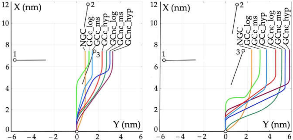
Figure 16.
Safe trajectories of the subject ship when passing one ship (J = 12) under conditions of good visibility at Ds = 1 nm (left) and restricted visibility at Ds = 3 nm (right), calculated using the cooperative and non-cooperative game control method with the collision risk model rj-logarithmic GCc_log and GCnc_log, mean square GCc_ms and GCnc_ms, and hyperbolic GCc_hyp and GCnc_hyp; for comparison, the trajectories of the non-game control NGC are presented.
Figure 16.
Safe trajectories of the subject ship when passing one ship (J = 12) under conditions of good visibility at Ds = 1 nm (left) and restricted visibility at Ds = 3 nm (right), calculated using the cooperative and non-cooperative game control method with the collision risk model rj-logarithmic GCc_log and GCnc_log, mean square GCc_ms and GCnc_ms, and hyperbolic GCc_hyp and GCnc_hyp; for comparison, the trajectories of the non-game control NGC are presented.
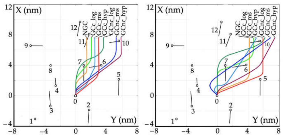
Figure 17.
Characteristics of the final deviation d of the subject ship’s safe trajectory as a function of the safe passing distance Ds for the cooperative GCc and non-cooperative GCnc control methods, using the logarithmic log, mean square ms, and hyperbolic hyp collision risk model: (a) J = 1; (b) J = 3; (c) J = 12.
Figure 17.
Characteristics of the final deviation d of the subject ship’s safe trajectory as a function of the safe passing distance Ds for the cooperative GCc and non-cooperative GCnc control methods, using the logarithmic log, mean square ms, and hyperbolic hyp collision risk model: (a) J = 1; (b) J = 3; (c) J = 12.
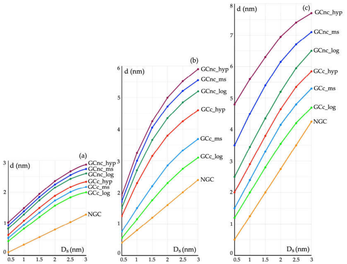
Figure 18.
Sensitivity characteristics of the final deviation d of the subject ship’s safe trajectory to changes in the safe distance Ds when passing J ships: (a) J = 1; (b) J = 3; (c) J = 12.
Figure 18.
Sensitivity characteristics of the final deviation d of the subject ship’s safe trajectory to changes in the safe distance Ds when passing J ships: (a) J = 1; (b) J = 3; (c) J = 12.
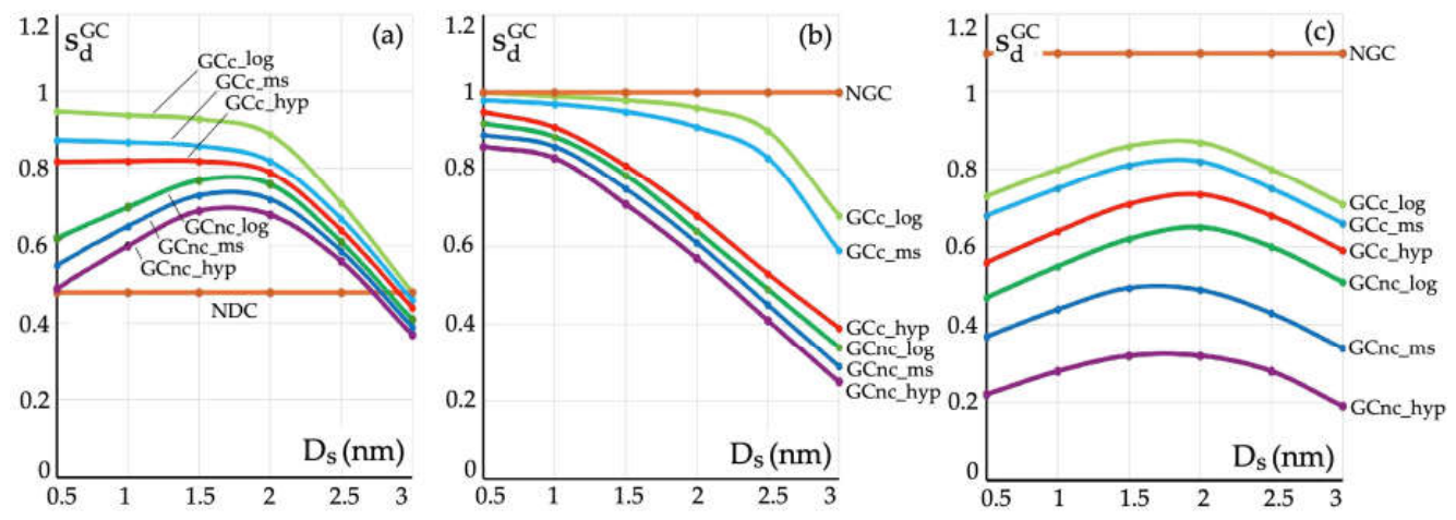
Figure 19.
Effectiveness characteristics s0 of the algorithms for the safe control of the subject ship, taking into account the movement of three other ships, depending on the state of the navigation situation represented by the value of the safe passing distance Ds according to COLREG for the methods GCnc, GCc, NDC, and as a reference kinematic NGC.
Figure 19.
Effectiveness characteristics s0 of the algorithms for the safe control of the subject ship, taking into account the movement of three other ships, depending on the state of the navigation situation represented by the value of the safe passing distance Ds according to COLREG for the methods GCnc, GCc, NDC, and as a reference kinematic NGC.
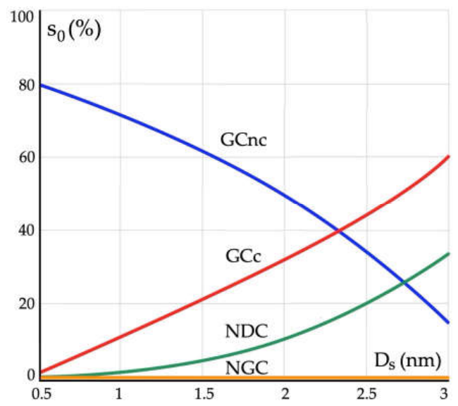

Table 1.
Data describing the navigational situations of the subject ship’s movement and the J ships it passes.
Table 1.
Data describing the navigational situations of the subject ship’s movement and the J ships it passes.
| Situation | Object Number j |
Speed Vj (kn) |
Course yj (deg) |
Coordinate Xj (nm) |
Coordinate Yj (nm) |
|---|---|---|---|---|---|
| J = 1 | 0 | 16.0 | 0 | 0 | 0 |
| 1 | 14.0 | 275 | 4.20 | 4.35 | |
| J = 3 | 0 | 20.0 | 0 | 0 | 0 |
| 1 | 14.5 | 89 | 6.40 | −5.60 | |
| 2 | 16.2 | 189 | 11.20 | 1.00 | |
| 3 | 16.1 | 199 | 7.27 | 1.53 | |
| J = 12 | 0 | 20.0 | 0 | 0 | 0 |
| 1 | 0 | 180 | −3.11 | −5.27 | |
| 2 | 15.9 | 183 | −1.99 | 1.73 | |
| 3 | 18.1 | 355 | −1.27 | −3.27 | |
| 4 | 7.8 | 355 | 1.55 | −2.64 | |
| 5 | 19.9 | 180 | 2.01 | 5.64 | |
| 6 | 14.5 | 80 | 3.64 | 1.73 | |
| 7 | 19.5 | 181 | 3.86 | 0.99 | |
| 8 | 0 | 1 | 3.91 | −3.27 | |
| 9 | 13.9 | 91 | 6.45 | −5.73 | |
| 10 | 11.3 | 80 | 6.90 | 4.36 | |
| 11 | 16.1 | 201 | 7.82 | 1.73 | |
| 12 | 17.1 | 191 | 9.36 | 0.55 |
Disclaimer/Publisher’s Note: The statements, opinions and data contained in all publications are solely those of the individual author(s) and contributor(s) and not of MDPI and/or the editor(s). MDPI and/or the editor(s) disclaim responsibility for any injury to people or property resulting from any ideas, methods, instructions or products referred to in the content. |
© 2026 by the authors. Licensee MDPI, Basel, Switzerland. This article is an open access article distributed under the terms and conditions of the Creative Commons Attribution (CC BY) license (http://creativecommons.org/licenses/by/4.0/).
Copyright: This open access article is published under a Creative Commons CC BY 4.0 license, which permit the free download, distribution, and reuse, provided that the author and preprint are cited in any reuse.