

Submitted:
07 August 2026
Posted:
10 August 2026
You are already at the latest version
Abstract
A non-sinusoidal regime is commonly found in power grids and affects the nominal operation and performance of industrial equipment supplied by the electrical network. The non-sinusoidal regime is mainly caused by nonlinear circuit elements, especially power-electronic devices. In real industrial cases, the harmonic content of voltage and current varies; consequently, the RMS values can change significantly, influencing both power flow and power quality. To determine these variations, this article proposes a method for analyzing the dependence between the harmonic weights of voltage and current and the sensitivities of reactive and apparent powers. After introducing dependency relationships between real, reactive, and apparent powers and harmonic weights, the method uses these relationships to calculate sensitivities when one or more parameters are modified. A numerical algorithm is implemented in MATLAB/Simulink to determine the sensitivities in a real case. The values obtained are compared with those directly calculated from measured data, and the small errors demonstrate the accuracy of the proposed method.
Keywords:
nonsinusoidal regime
; harmonic weight
; sensitivity analysis
; reactive power
; apparent power
; numerical algorithm
1. Introduction
Nowadays, electrical power systems are subjected to a nonsinusoidal regime that produces voltage and current harmonics and interharmonics,with detrimental effects on equipment. The most significant drawbacks are increased losses in power cables and transformers, motor overheating, degradation of dielectric insulation, electromagnetic interference, and errors in energy measurement at the level of revenue meters [1]. Moreover, the fluctuations associated with the nonsinusoidal regime directly affect voltage stability, can trigger random protection tripping, and, overall, decrease reliability and reduce the lifespan of electrical apparatus [2]. Analyzing the real, apparent and reactive power in the nonsinusoidal regime is very important. To avoid undesired effects such as overheating and uncontrolled magnetic excitations, or to limit additional losses [3,4], one specifies the power conductors, transformers’ windings, and filters by inputting an augmented apparent power value. Reactive power assessment is key to ensuring voltage stability and maintaining power factor in the presence of nonlinear loads. Correctly implemented reactive power compensation can decrease the capacitive battery rating by 5-7% and reduce total power supply losses [5,6]. The calculation algorithms adapted to the classical theory of power measurement can significantly improve the accuracy of reactive power meters, achieving errors of 1% or less, even when the total harmonic distortion of the voltage (THDu) or the total demand distortion of the current (THDi) exceeds 20%. Nonlinear loads and power converters, which are common in industrial, commercial, and residential electrical installations, cause the most voltage and current distortions [7–9]. Following the previous considerations, a sensitivity analysis applied to the nonsinusoidal regime quantifies the dependency between the variations in voltage and current harmonics and the electrical system response by computing the derivatives of the network transfer functions with respect to the input parameters (harmonics magnitudes and phases) [10–12]. Additionally, techniques specifically developed to address this area enable detailed sensitivity analysis using real acquired data via appropriate measurements, thereby emphasizing the importance of each harmonic parameter across different operating scenarios [13–15]. Unlike the previously mentioned works the main subject of the article is the determination of the influence of the variation of the voltage, current and phase shift angle weights (defined in the following as parameters) on the real, reactive and apparent powers absorbed by an industrial consumer. On a real circuit operating in non-sinusoidal mode, two modifications were introduced - which could very possibly appear as faults - and the measured data were used to calculate the sensitivities associated with the powers. In this sense, new calculation relations for the reactive and apparent powers are introduced based on these parameters, which are then used to calculate the sensitivities [16]. In a numerical algorithm, the variations of one or more parameters are considered. Section II presents the mathematical formulation of the method and the relationships for calculating real, reactive, and apparent power using sensitivities. Section III analyses a real industrial case, discusses the obtained results, and identifies errors. Finally, Section IV concludes.
Figure 1 displays a summary of the main types of equipment that generates nonsinusoidal waveforms.
2. Mathematical Formulation
One can define the first-order sensitivity of function F of 3n variables concerning the variation of one variable xk as follows [16]:
We considered that the set of variables on which the function F depends can be divided into 3 disjoint subsets, X,Y,Z each containing the same number n of variables. This classification of variables will be used in the following. Similarly, 2-order sensitivity concerning the variation of two variables (xk, ym) from two subsets can be defined as follows [17]:
where the variables k, m=1,…,n. In this manner, one can express the sensitivity of the function F to the variation of multiple variables. Thus, for the simultaneous variation of all variables x, y, z from the 3 disjoint subsets, the 3-order sensitivity is expressed as a Taylor linearization in connection to the parameters k, m, q:
The voltage and current at the terminals of a receiver operating in a nonsinusoidal regime appear in the time domain in the form of their Fourier decomposition, expressed by [18,19]:
where n represents the number of harmonics. Mathematical relationships (4)-(6) highlight the rms values of the voltage harmonics Uk, current harmonics Ik, respectively, and the phase shift angle between the voltage and current of each harmonic order. The latter represents the difference between the initial voltage harmonic phase and current harmonic phase . In industrial applications, when encountering a nonsinusoidal regime, aside from the fundamental harmonic, the magnitudes and phase shifts of the voltage and current harmonics vary due to the nonlinearity of the loads and the unbalanced power network character. The time-dependent values of the real, reactive, respectively, the apparent power absorbed by a consumer operating in a nonsinusoidal regime, strongly depend on three categories of parameters which constitute the 3 disjoint subsets specified above. These parameters are [20]:
- the voltage harmonic relative weights with respect to the voltage fundamental:
- the current harmonic relative weights with respect to the current fundamental:
- the angle between the voltage and current harmonics
- for that one can compute cosine and sine as given below:
Considering the parameters described above, new relations can be obtained to express the real, reactive and apparent power:
where U1 and I1 represent the rms values of voltage respectively current of the fundamental frequency. Analyzing relations (11) - (13), the dependencies of P, Q and Sa on the weights and phase shift angles suggest the use of the sensitivities defined by relation (3). Considering that the parameters r,p, described by relations (7)-(10) represent the subsets of variables x, y, z, and F represents P, Q, respectively, Sa, then the 3-order sensitivities related to the real and reactive power respectively the 2-order sensitivity related to apparent power, are calculated starting from (3) and using relations (11)-(13) as follows:
Obviously, any combination of parameters r,p,, can be chosen that changes, for any harmonic including the same one, when calculating the sensitivities. In particular presuming that only two parameters vary simultaneously, compared to the initial values, for example for the same k-harmonic rk and pk, then the 2-order second sensitivity regarding the real, reactive and apparent powers is calculated based on relations (14)-(16). Results the second-order sensitivities:
If one or more parameters do not change from their initial values, then the respective term(s) is/are missing (is/are 0) from the sum. In industrial applications we can define an initial regime with the initial values of parameters r, p, . Such a regime can be considered the nominal operating regime of the load, and the initial parameters are measured by a data acquisition system. It is noted with and the new values of relative harmonics weight of voltage and current respectively of the phase angle that change compared to the initial ones.
Three computation methods are compared. Method 1 (direct computation) evaluates P, Q, and Sa by directly applying the values of the initially harmonic parameters using (11)-(13).
Method 2 implies the recomputation of the powers after modifying a selected subset of relative values of harmonic using the same relations (11)-(13). these values.
Method 3 considers the sensitivity-based estimation for the same parameters’ changing using (14)-(16), where the terms in the sums corresponding to the parameters that do not change are zero. Then at the next step of numerical algorithm, one can calculate new values of the real Pcalc., reactive Qcalc., respectively apparent power Sa,calc. using the method 3, according to the variation of parameters. The following relations can be introduced:
where P, Q and S represent the initial values of real, reactive, and apparent power, calculated with method 1. To validate the proposed method, the absolute error can be defined as the difference between the computed in method 1 and the values of powers calculated with method 3 that use the sensitivity method:
The relative errors concerning the increase or decrease of real, reactive and apparent power when parameters are modified are obtained with the relations below:
3. Case Study and Results
For the case study, the power circuit represented in Figure 2 consists of a twelve-pulse uncontrolled rectifier energized through two transformers of equal rating. To obtain the 30 -degree phase shift between the three-phase output voltages at the transformers’ secondary outputs one transformer has a delta-delta winding connection, whereas the other one has a delta-star configuration. The main power supply comes from a system that is intrinsically slightly polluted with harmonics, due to the proximity of a light-rail system.
In Case I the circuit is symmetrical and operated in normal conditions. In Case II there are non-symmetries, simulated as possible faults, by artificially inserting inductivities in series with one phase, together with the removal of one diode (marked as DA2-).
The circuit, supplied by 3x208V/60Hz consists of one delta-delta 3kVA, 3x208V/104V, 60Hz transformer, one delta-star 3kVA, 3x208V/104V, 60Hz transformer, two uncontrolled three-phase bridge rectifiers, and resistive load of 400 ohms (for the rectifiers). The inductor introduced to create unbalanced voltages at the input to the delta – delta transformer has an air core and a value of 0.012H. All measurements were performed using a Fluke 196C Scopemeter, whereas waveform acquisition and harmonic analysis were performed using the dedicated software package Fluke View associated with the meter. To obtain the line to neutral voltages, one connected a three- phase high impedance load at the output of the three-phase power supply, with direct access to its isolated neutral. All three phase line-to-neutral voltages, together with the line currents (uA and iA ,uB and iB, respectively uC and iC) have been acquired using equipment from a specialized laboratory at the Northern Alberta Institute of Technology. Consequently, the phase notations (A, B, C) conform to NEMA standards. The sampling frequency used in signal acquisition is 10 kHz, and the measurements show the magnitudes of the two non-sinusoidal regimes, Case I and Case II in the steady state, without presenting the transient regime. The waveforms obtained with the Scopemeter are compared to the ones computed following the harmonic decomposition. In Figure 3 and Figure 4, one can compare the phase A line to neutral voltage obtained through direct measurement, respectively calculated following the harmonic decomposition in conditions of completely symmetrical circuit (Case I), respectively when the circuit is unsymmetric by the intentional introduction of inductivity in series through phase A, respectively by removing the diode DA2- (Case II). The second case delivers harmonic parameters, considered for determining the powers in both cases: calculated with modified parameters, respectively with respect to sensitivities. The measured and computed parameters of the harmonics of phase A in Case I and Case II are presented in Table I and Table II, respectively.
For phase B the voltage and current graphs in both cases studied normal operating conditions and non-symmetrical regime are represented in Figure 5 and Figure 6, while the associated values of the harmonics’ parameters are specified and calculated in Table III and Table IV, respectively.
The voltage and current graphs for phase C in both cases studied normal operating conditions and non-symmetrical regime are shown in Figure 7 and Figure 8, while the associated values of the harmonics’ parameters are presented and calculated in Table V and Table VI, respectively.
To determine the sensitivities with relations (14)-(16), Tables VII a, b, and c present synthetically the values of the parameters r, p, and that change in Case II compared to Case I and that will be considered in the calculation. For a correct and simple presentation of the parameters that will be considered and are changed, they have been highlighted in turquoise in Tables VII a,b,c, and the other terms associated with the parameters that do not change will be null. The numerical algorithm contains a procedure for comparing the values of the parameters in the 2 cases and for choosing the parameters that change. In the studied cases, the only parameter that does not change is r attached to the 12th and 14th harmonics of phase A, the 12th harmonic of phase B, and the 10th and 14th harmonics of phase C. All other parameters change in Case II compared to Case I.

Table VII-a.
Comparison of relative harmonic parameters for phase A (Case I vs. Case II).
| Harmonic order |
r | p | [deg] | [deg] | ||
|---|---|---|---|---|---|---|
| 1 | 1.0000 | 1.0000 | 1.0000 | 1.0000 | 32.3 | 35.51 |
| 2 | 0.0016 | 0.0041 | 0.0793 | 10.4223 | 16.07 | 11.17 |
| 3 | 0.0024 | 0.0041 | 0.7928 | 2.8751 | 7.54 | 7.46 |
| 4 | 0.0008 | 0.0017 | 0.1586 | 1.0782 | 9.25 | 3.57 |
| 5 | 0.0163 | 0.0132 | 4.4395 | 4.1330 | 2.46 | 16.26 |
| 6 | 0.0000 | 0.0017 | 0.1586 | 1.0782 | 5.62 | 7.03 |
| 7 | 0.0073 | 0.0083 | 0.4757 | 0.6289 | 7.57 | 9.89 |
| 8 | 0.0016 | 0.0017 | 0.1586 | 1.3477 | 2.74 | 6.63 |
| 9 | 0.0016 | 0.0017 | 0.2378 | 0.5391 | 0.15 | -14.67 |
| 10 | 0.0000 | 0.0025 | 0.0793 | 0.8086 | 20.71 | -10.97 |
| 11 | 0.0057 | 0.0091 | 2.8540 | 2.6954 | -15.02 | -10.18 |
| 12 | 0.0008 | 0.0008 | 0.0793 | 0.5391 | -0.24 | -8.55 |
| 13 | 0.0065 | 0.0091 | 1.9026 | 1.2579 | 3.36 | -2.48 |
| 14 | 0.0008 | 0.0008 | 0.0793 | 0.5391 | 2.42 | 5.35 |
| 15 | 0.0008 | 0.0017 | 0.2378 | 0.6289 | 5.2 | -7.12 |
Table VII-b.
Comparison of relative harmonic parameters for phase B (Case I vs. Case II).
| Harmonic order |
r | p | [deg] | [deg] | ||
|---|---|---|---|---|---|---|
| 1 | 1.0000 | 1.0000 | 1.0000 | 1.0000 | 32.05 | 31 |
| 2 | 0.0016 | 0.0008 | 0.4237 | 3.3091 | 13.28 | 12.22 |
| 3 | 0.0008 | 0.0017 | 0.5085 | 2.7300 | 11.38 | 12.32 |
| 4 | 0.0008 | 0.0025 | 0.0847 | 0.6618 | 10.5 | 12.63 |
| 5 | 0.0164 | 0.0173 | 4.8305 | 4.4672 | 8.66 | 17.7 |
| 6 | 0.0008 | 0.0017 | 0.0847 | 1.3236 | 5 | 9.47 |
| 7 | 0.0082 | 0.0058 | 0.5932 | 0.9100 | 7.25 | 11.98 |
| 8 | 0.0016 | 0.0017 | 0.1695 | 0.5791 | -4.97 | -3.04 |
| 9 | 0.0016 | 0.0017 | 0.1695 | 1.1582 | -0.72 | -6.29 |
| 10 | 0.0008 | 0.0017 | 0.0847 | 0.1655 | 12.65 | 56.47 |
| 11 | 0.0066 | 0.0050 | 3.3898 | 2.8127 | 12.85 | -14.44 |
| 12 | 0.0008 | 0.0008 | 0.0847 | 0.7445 | -10.39 | -2.93 |
| 13 | 0.0049 | 0.0083 | 2.3729 | 1.4064 | -1.15 | 0.18 |
| 14 | 0.0008 | 0.0025 | 0.1695 | 0.3309 | -5.75 | -1.46 |
| 15 | 0.0016 | 0.0000 | 0.1695 | 0.4136 | 16.9 | 5.69 |
Table VII-c.
Comparison of relative harmonic parameters for phase C (Case I vs. Case II).
| Harmonic order |
r | p | [deg] | [deg] | ||
|---|---|---|---|---|---|---|
| 1 | 1.0000 | 1.0000 | 1.0000 | 1.0000 | 29.51 | 36.32 |
| 2 | 0.0008 | 0.0033 | 0.1613 | 10.0639 | 12.21 | 15.15 |
| 3 | 0.0024 | 0.0016 | 0.6453 | 0.6390 | 9.54 | 9.48 |
| 4 | 0.0000 | 0.0016 | 0.1613 | 1.5176 | 6.55 | 12.18 |
| 5 | 0.0155 | 0.0172 | 4.7588 | 3.1949 | 3.24 | -3.59 |
| 6 | 0.0000 | 0.0016 | 0.1613 | 1.3578 | 4.32 | 10.39 |
| 7 | 0.0065 | 0.0057 | 0.4033 | 1.5974 | 1.92 | 11.57 |
| 8 | 0.0008 | 0.0016 | 0.0807 | 1.1182 | -3.89 | 14.97 |
| 9 | 0.0008 | 0.0016 | 0.1613 | 0.8786 | -22.09 | 34.58 |
| 10 | 0.0016 | 0.0016 | 0.0807 | 0.1597 | 20.84 | 4.43 |
| 11 | 0.0073 | 0.0106 | 2.9037 | 0.7188 | -24.71 | 3.77 |
| 12 | 0.0000 | 0.0008 | 0.0807 | 0.3195 | 7.56 | 11.19 |
| 13 | 0.0049 | 0.0057 | 2.0971 | 1.5974 | 6.73 | -1.68 |
| 14 | 0.0008 | 0.0008 | 0.0807 | 0.5591 | -10.65 | 0.05 |
| 15 | 0.0000 | 0.0008 | 0.1613 | 0.2396 | -4.71 | 7.58 |
The flowchart shown in Figure 9, presents the steps for implementing the algorithm in MATLAB/Simulink, to calculate real, reactive, and apparent powers using three methods: direct calculation using the parameters of normal conditions respectively the modified parameters, and the calculation with sensitivity method.
The direct method computation of the powers in the two cases uses relations (11)-(13) and parameters and for Case I, respectively and for Case II. Table VIII presents the numerical results obtained for each phase.
When analyzing the two cases, one can conclude that the most significant modifications encounter current harmonics, respectively harmonics 2 and 5. Also, the fifth harmonic of the phase voltage, suffers modifications. The parameters of interest for the sensitivity analysis, subjecting the real, reactive and apparent power for all three phases are: r2, p2, respectively r5and p5. The new values calculated utilizing sensitivities are compared with the power values recorded in case II. The harmonic parameters used in the sensitivity analysis are summarized in Tables VII-a–VII-c.
The sensitivity method used relations (14)-(16) in which only the parameters and that change appear. Relations (14) and (15) are applied for the 3-order sensitivities related to the real and reactive power and relation (16) used the 2-order sensitivity related to apparent power. For example, in the calculation of the sensitivity SP related to the real power: for phase A all the terms containing r12 and r14, for phase B all the terms containing r12and for phase C all the terms containing r10 and r14 are zero. Then using relations (20)-(22) the real, reactive and apparent powers are computed. The results for each phase are presented synthetically in Table IX.
The absolute error (23)-(25) and the relative errors (26)-(28) of the proposed method, for each phase, are synthetically presented in Table X.
Several conclusions can be drawn from the analysis of the case study and the calculations performed.
First, it is found that the modifications made to the initial circuit, i.e. the introduction of inductivity in series through phase A, respectively by removing the diode DA , are not found in all parameters nor in all phases equally. Tables VII - a, b, c shows that only a small part of the relative parameters r, p, and changes in Case II compared to Case I of the nominal regime. Thus, in phases A and C, 2 parameters are not changed and in phase B only one. It can be said that phase B is less sensitive to the variations of the parameters.
Then the resistive-inductive character of the initial circuit is preserved in Case II, which results from the analysis of the values calculated from table VIII, so all the reactive power values being positive.
Regarding the errors, it is found that their values are positive and negative. For absolute errors, positive values show a higher value of the powers calculated with the direct method using the modified parameters compared to the powers calculated with the sensitivity method. Otherwise, the absolute error values are negative. The positive or negative sign of the absolute errors is also preserved in the case of relative errors.
As can be seen from table X, all the values of both absolute and relative errors are small, which shows a good accuracy of the method. Moreover, the absolute and relative errors of the powers of phases A and C are slightly higher than those of the phase B, which indicates the higher sensitivity of this phase, confirming the strong modification of 58 parameters, as can be seen from tables VII-a and VII-c.
4. Conclusions
The sensitivity analysis represents an efficient tool for characterizing the influence of the variation of electrical network parameters on the real, reactive, and apparent power absorbed by a load operating in a nonsinusoidal regime. New relationships of real, reactive and apparent power based on the sensitivity method, in conditions of modifying one or more parameters simultaneously, are proposed. If the voltage and current signals exhibit time-varying harmonics, the proposed method still provide reliable results if online data acquisition system, for example SCADA, is used to determine the initial and the modified parameters, and the values of powers. The modifiable parameters are defined as relative magnitudes of the values of voltage and current harmonics, respectively of the phase shifts between voltage and current. Used online data acquisition system, for example SCADA, the initial and the modified parameters can be used for a numerical algorithm which determines the values of the powers. The calculation of the powers is done using the direct method with initial and modified parameters, respectively the method of sensitivities. The results obtained for the three-phase circuit studied showed a good accuracy of the sensitivity method and specified the degree of sensitivity of each parameter and phase related to the modification of the circuit elements.
Additionally, sensitivity analysis is essential in harmonic filter design and selecting the optimal methods to address harmonic mitigation and eliminate the associated drawbacks properly. Furthermore, the newly generated optimization functions aim to determine the appropriate limits of the voltage, current, and phase shift so that the quality of the energy would be compatible with IEEE 519-2022for solving all these issues recorded for electric power networks operating in nonsinusoidal regime.
Author Contributions
Conceptualization HA, MS, methodology HA, MS, PA, SD, EC, ED, DM, software PA, ED, validation EC, formal analysis HA, MS,DM, investigation PA, SD, ED, resources SD, data curation PA, writing—original draft preparation MS, writing—review and editing HA, visualization SD,EC,PA supervision HA.
Funding
This research received no external funding.
Institutional Review Board Statement
Not applicable.
Informed Consent Statement
Not applicable.
Data Availability Statement
The data supporting the findings of this study are available from the corresponding author upon reasonable request. Please revise this statement if the data are deposited in a public repository.
Conflicts of Interest
The authors declare no conflicts of interest.
References
- Rigitano, D.; Cianca, A. D.; Kolsteren, M. Novel indices for power quality assessment of non-linear loads. Electr. Power Syst. Res. 2024, 214, 109107. [Google Scholar]
- Nicolae, P.M.; Nicolae, I.D.; Nicolae, M.Ş. Powers and Power Factor in Non-Sinusoidal and Non-Symmetrical Regimes in Three-Phase Systems. Energies 2022, 15, 5130. [Google Scholar]
- Madnani, Rohan; Mishra, Mahesh; Ghosh, Arindam. Reactive Power Evaluation for Non-Sinusoidal Single Phase Systems. IEEE Trans. Circuits Syst. I Regul. Pap. 2024, 1–12. [Google Scholar] [CrossRef]
- Michalec, Ł.; et al. Impact of Harmonic Currents of Nonlinear Loads on Power Quality of a Low Voltage Network–Review and Case Study. Energies 2021, 14, 3665. [Google Scholar]
- El-Goharey, H.S.K.; Mamdouh, W.M. On-line analysis of power quality problems in non-sinusoidal/non-linear loads. Ain Shams Eng. J. 14, 2–23.
- Kováč, M.; et al. Reactive Power and Energy Instrument’s Performance in Non-Sinusoidal Conditions. Meas. Sci. Rev. 2023, 23, 19–31. [Google Scholar] [CrossRef]
- Alduraibi, A.; Yaghoobi, J.; Zare, F. Impacts of grid voltage harmonics amplitude and phase angle values on power converters in distribution networks. IEEE Access 2021, 9, 92017–92029. [Google Scholar] [CrossRef]
- IEEE Std 519-2022; IEEE Standard for Harmonic Control in Electric Power Systems. in (Revision of IEEE Std 519-2014).
- Vlahinic, S.; Brnobic, D.; Stojkovic, N. Indices for Harmonic Distortion Monitoring of Power Distribution Systems. IEEE Trans. Instrum. Meas. 2009, 58, 1771–1777. [Google Scholar] [CrossRef]
- Diaconu, L. Sensitivity Analysis of the Linear Networks in Non-sinusoidal Regime. In Proceedings of the International Conference on Electromechanical and Power Systems, 2011. [Google Scholar]
- SensitivityAnalysisand Power Systems: CanWe Bridge theGap? A Review and a GuidetoGettingStarted - MDPI. Available online: https://www.mdpi.com/1996-1073/14/24/8274 (accessed on 5 May 2025).
- PositionPaper: BridgingtheGapBetweenMachineLearningandSensitivityAnalysis - arXiv. 2024, 1–7. Available online: https://arxiv.org/pdf/2312.13234 (accessed on 5 May 2025). [PubMed]
- A Review of Global SensitivityAnalysisMethodsand a comparative case study on Digit Classification. arXiv. Available online: https://arxiv.org/html/2406.16975v1 (accessed on 5 May 2025).
- SystemsAnalysis in Electric Power Sector Modeling: A Review of the Recent LiteratureandCapabilities of SelectedCapacity Plan - EPRI. Available online: https://restservice.epri.com/publicdownload/000000003002011102/0/Product (accessed on 5 May 2025).
- Blenk, T.; Weindl, C. Development of Methods for SensitivityAnalysis of Electrical Energy NetworksandSystemswithin State Space. Energies 2024, 17, 4489. [Google Scholar] [CrossRef]
- Andrei, H.; Spinei, F.; Cepisca, C. On sensitivities in steady state circuits. In Signals, Circuits and Systems, 2003. SCS 2003; Iasi, Romania, 2003; Volume 2, pp. 469–472. [Google Scholar] [CrossRef]
- Caciula, I.; Andrei, H.; Diaconu, E.; Puchianu, D.C. Numerical Method Analysis of Nonlinear Elements Behavior in Non-sinusoidal State. 2023 13th ATEE, Bucharest, Romania, 2023; pp. 1–6. [Google Scholar] [CrossRef]
- Iordache, M.; Stãnculescu, M.; Andrei, P.; Bobaru, L.; Andrei, H.; Diaconu, E. Equivalent Models of Nonlinear Circuit Elements in Nonsinusoidal Regime. 2023 10th International Conference on Modern Power Systems (MPS), Cluj-Napoca, Romania, 2023; pp. 1–5. [Google Scholar] [CrossRef]
- de Villiers, M.; Mukundi Mwaniki, F. Single-Phase Grid-Connected Inverter Parameter Sensitivity Analysis using Wide-band Impedance Estimations. 2025 33rd Southern African Universities Power Engineering Conference (SAUPEC), Pretoria, South Africa, 2025; pp. 1–6. [Google Scholar]
- Andrei, P.; Deleanu, S.; Diaconu, E.; Gheorghe, A.; Stănculescu, M.; Cazacu, E.; Andrei, H. New Method for Sensitivity Analysis of Reactive and Apparent Power in Non-Sinusoidal State. 2025 17th International Conference on Electronics, Computers and Artificial Intelligence (ECAI), Targoviste, Romania, 2025; pp. 1–6. [Google Scholar]
Figure 1.
The main types of equipment that generate nonsinusoidal waveforms.
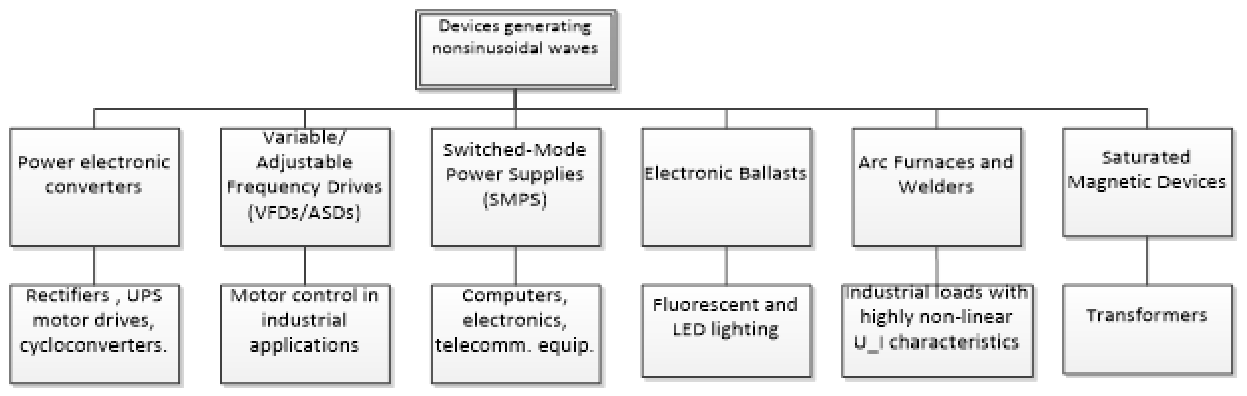
Figure 2.
The studied three-phase circuit.
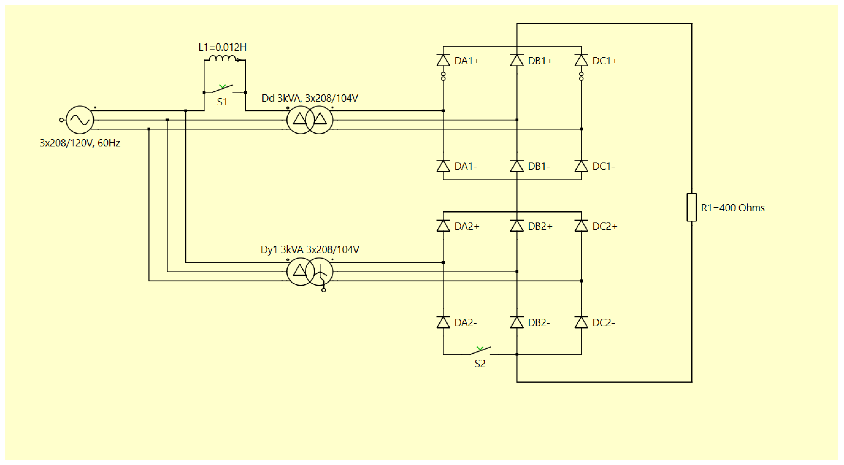
Figure 3.
(van) and (ias): (a) measured values; (b) synthesized signals following the harmonic decomposition—Case I.
Figure 3.
(van) and (ias): (a) measured values; (b) synthesized signals following the harmonic decomposition—Case I.
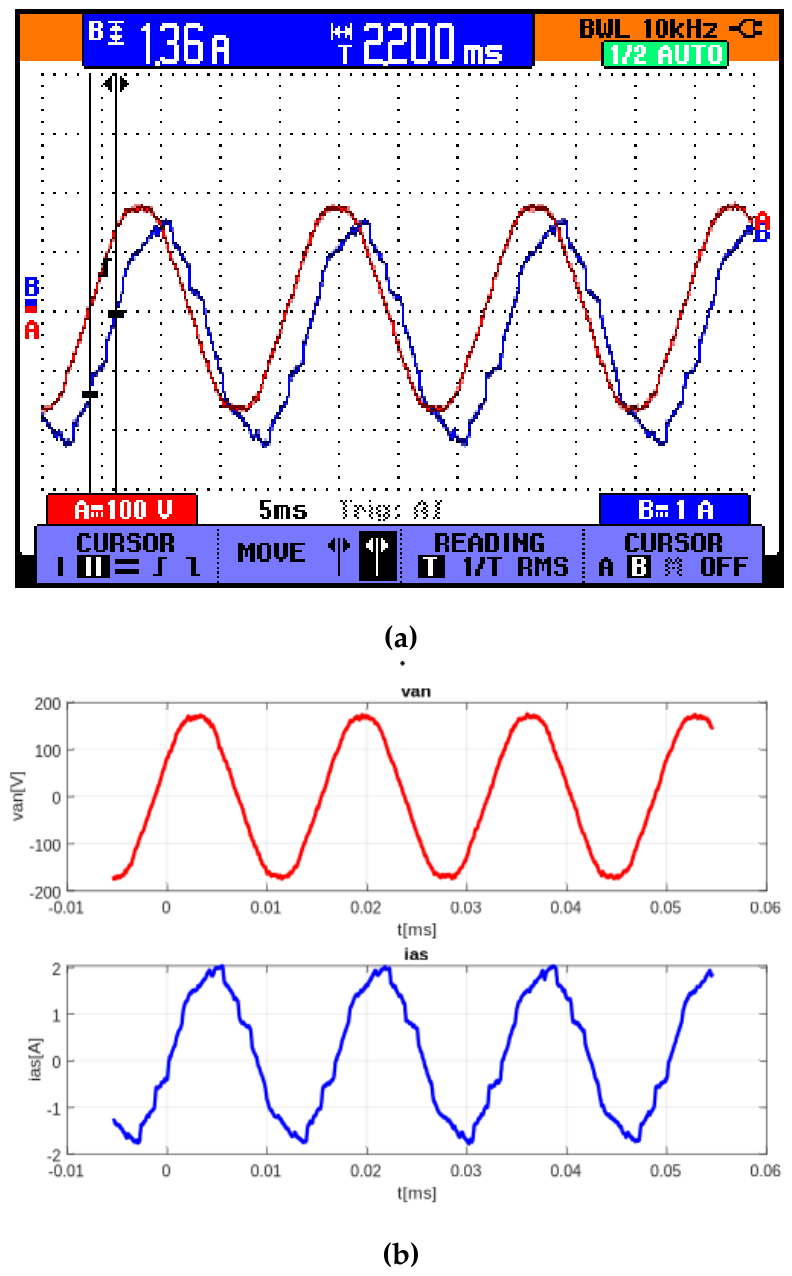
Figure 4.
(van) and (ias): (a) measured values; (b) synthesized signals following harmonic decomposition in unsymmetrical conditions (coils inserted into line A and diode DA2 missing)–Case II.
Figure 4.
(van) and (ias): (a) measured values; (b) synthesized signals following harmonic decomposition in unsymmetrical conditions (coils inserted into line A and diode DA2 missing)–Case II.
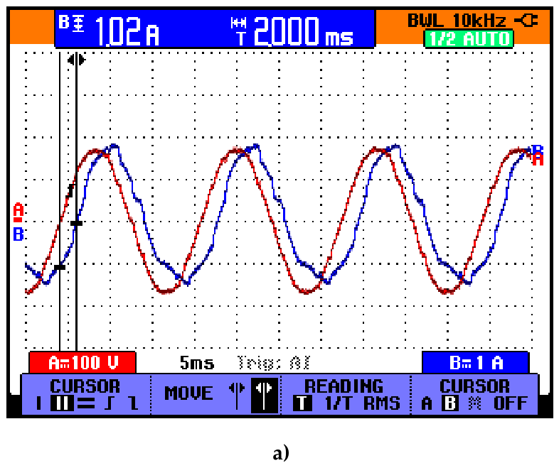
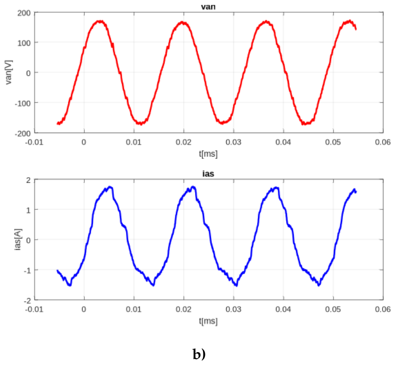
Figure 5.
(vbn, red) and (ibs, blue), measured values—Case I.
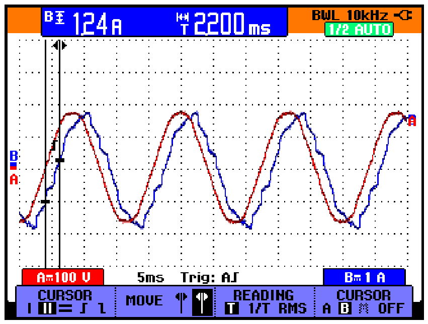
Figure 6.
(vbn, red) and (ibs, blue), measured values—Case II.
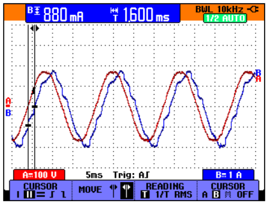
Figure 7.
(vcn, red) and (ics, blue), measured values—Case I.
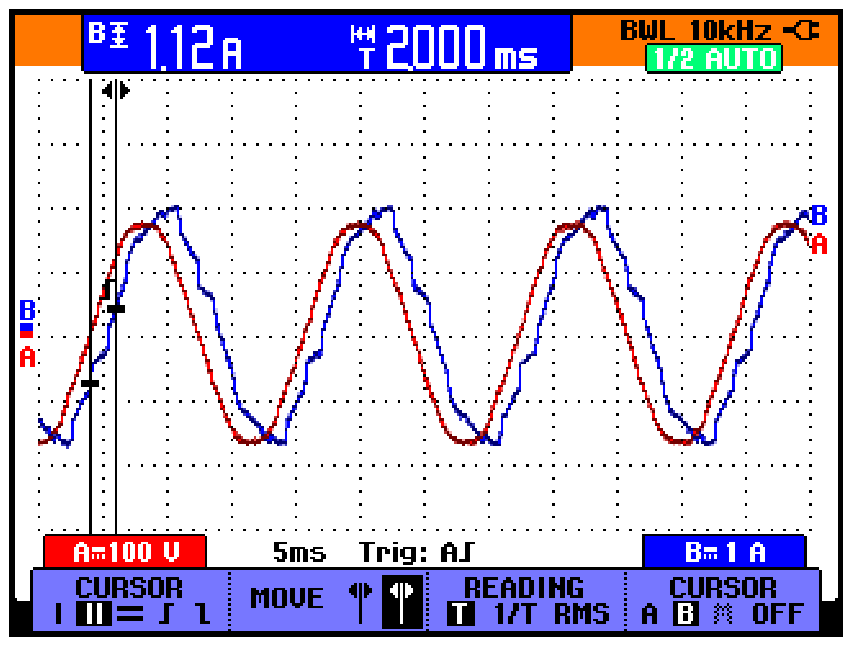
Figure 8.
(vcn, red) and (ics, blue), measured values—Case II.
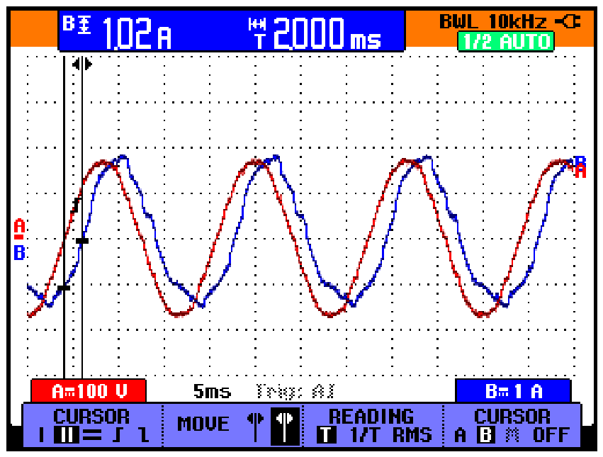
Figure 9.
Flowchart of the numerical algorithm.
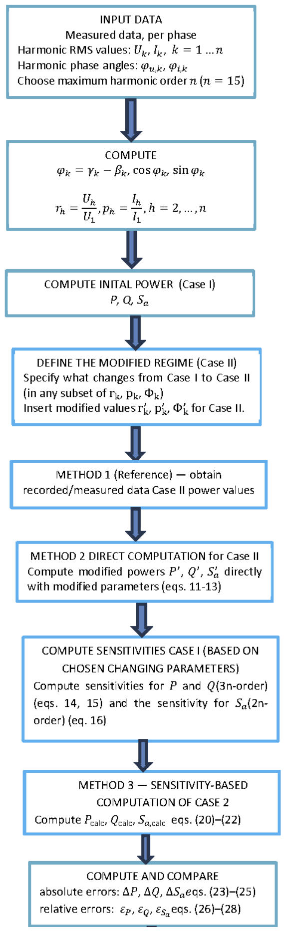
Table I.
Voltage and current values of harmonics for phase A in normal operating conditions—Case I.
| Harmonic order |
UArms (V) | r | p | IArms (A) | Ak [deg] |
|---|---|---|---|---|---|
| 1 (60Hz) | 123V | 1.0000 | 1.0000 | 1.261 | 32.3 |
| 2 | 0.2 | 0.0016 | 0.0793 | 0.1 | 16.07 |
| 3 | 0.3 | 0.0024 | 0.7928 | 1 | 7.54 |
| 4 | 0.1 | 0.0008 | 0.1586 | 0.2 | 9.25 |
| 5 | 2 | 0.0163 | 4.4395 | 5.6 | 2.46 |
| 6 | 0 | 0.0000 | 0.1586 | 0.2 | 5.62 |
| 7 | 0.9 | 0.0073 | 0.4757 | 0.6 | 7.57 |
| 8 | 0.2 | 0.0016 | 0.1586 | 0.2 | 2.74 |
| 9 | 0.2 | 0.0016 | 0.2378 | 0.3 | 0.15 |
| 10 | 0 | 0.0000 | 0.0793 | 0.1 | 20.71 |
| 11 | 0.7 | 0.0057 | 2.8540 | 3.6 | -15.02 |
| 12 | 0.1 | 0.0008 | 0.0793 | 0.1 | -0.24 |
| 13 | 0.8 | 0.0065 | 1.9026 | 2.4 | 3.36 |
| 14 | 0.1 | 0.0008 | 0.0793 | 0.1 | 2.42 |
| 15 | 0.1 | 0.0008 | 0.2378 | 0.3 | 5.2 |
Table II.
Voltage and current values of harmonics for phase A in non-symmetrical conditions—Case II.
Table II.
Voltage and current values of harmonics for phase A in non-symmetrical conditions—Case II.
| Harmonic order |
UArms (V) | IArms (A) | [deg] | ||
|---|---|---|---|---|---|
| 1 (60Hz) | 121.1V | 1.0000 | 1.0000 | 1.113 | 35.51 |
| 2 | 0.5 | 0.0041 | 10.4223 | 11.6 | 11.17 |
| 3 | 0.5 | 0.0041 | 2.8751 | 3.2 | 7.46 |
| 4 | 0.2 | 0.0017 | 1.0782 | 1.2 | 3.57 |
| 5 | 1.6 | 0.0132 | 4.1330 | 4.6 | 16.26 |
| 6 | 0.2 | 0.0017 | 1.0782 | 1.2 | 7.03 |
| 7 | 1 | 0.0083 | 0.6289 | 0.7 | 9.89 |
| 8 | 0.2 | 0.0017 | 1.3477 | 1.5 | 6.63 |
| 9 | 0.2 | 0.0017 | 0.5391 | 0.6 | -14.67 |
| 10 | 0.3 | 0.0025 | 0.8086 | 0.9 | -10.97 |
| 11 | 1.1 | 0.0091 | 2.6954 | 3 | -10.18 |
| 12 | 0.1 | 0.0008 | 0.5391 | 0.6 | -8.55 |
| 13 | 1.1 | 0.0091 | 1.2579 | 1.4 | -2.48 |
| 14 | 0.1 | 0.0008 | 0.5391 | 0.6 | 5.35 |
| 15 | 0.2 | 0.0017 | 0.6289 | 0.7 | -7.12 |
Table III.
Voltage and current harmonics for phase B in normal operating conditions—Case I.
| Harmonic order |
UBrms (V) | r | p | IBrms (A) | Bk[deg] |
|---|---|---|---|---|---|
| 1 (60Hz) | 122.1 | 1.0000 | 1.0000 | 1.18 | 32.05 |
| 2 | 0.2 | 0.0016 | 0.4237 | 0.5 | 13.28 |
| 3 | 0.1 | 0.0008 | 0.5085 | 0.6 | 11.38 |
| 4 | 0.1 | 0.0008 | 0.0847 | 0.1 | 10.5 |
| 5 | 2 | 0.0164 | 4.8305 | 5.7 | 8.66 |
| 6 | 0.1 | 0.0008 | 0.0847 | 0.1 | 5 |
| 7 | 1 | 0.0082 | 0.5932 | 0.7 | 7.25 |
| 8 | 0.2 | 0.0016 | 0.1695 | 0.2 | -4.97 |
| 9 | 0.2 | 0.0016 | 0.1695 | 0.2 | -0.72 |
| 10 | 0.1 | 0.0008 | 0.0847 | 0.1 | 12.65 |
| 11 | 0.8 | 0.0066 | 3.3898 | 4 | 12.85 |
| 12 | 0.1 | 0.0008 | 0.0847 | 0.1 | -10.39 |
| 13 | 0.6 | 0.0049 | 2.3729 | 2.8 | -1.15 |
| 14 | 0.1 | 0.0008 | 0.1695 | 0.2 | -5.75 |
| 15 | 0.2 | 0.0016 | 0.1695 | 0.2 | 16.9 |
Table IV.
Voltage and current harmonics for phase B in non-symmetrical conditions—Case II.
| Harmonic order |
UBrms (V) | IBrms (A) | Bk [deg] | ||
|---|---|---|---|---|---|
| 1 (60Hz) | 121.2V | 1.0000 | 1.0000 | 1.209 | 31 |
| 2 | 0.1 | 0.0008 | 3.3091 | 4 | 12.22 |
| 3 | 0.2 | 0.0017 | 2.7300 | 3.3 | 12.32 |
| 4 | 0.3 | 0.0025 | 0.6618 | 0.8 | 12.63 |
| 5 | 2.1 | 0.0173 | 4.4672 | 5.4 | 17.7 |
| 6 | 0.2 | 0.0017 | 1.3236 | 1.6 | 9.47 |
| 7 | 0.7 | 0.0058 | 0.9100 | 1.1 | 11.98 |
| 8 | 0.2 | 0.0017 | 0.5791 | 0.7 | -3.04 |
| 9 | 0.2 | 0.0017 | 1.1582 | 1.4 | -6.29 |
| 10 | 0.2 | 0.0017 | 0.1655 | 0.2 | 56.47 |
| 11 | 0.6 | 0.0050 | 2.8127 | 3.4 | -14.44 |
| 12 | 0.1 | 0.0008 | 0.7445 | 0.9 | -2.93 |
| 13 | 1 | 0.0083 | 1.4064 | 1.7 | 0.18 |
| 14 | 0.3 | 0.0025 | 0.3309 | 0.4 | -1.46 |
| 15 | 0 | 0.0000 | 0.4136 | 0.5 | 5.69 |
Table V.
Voltage and current harmonics for phase C in normal operating conditions—Case I.
| Harmonic order |
UCrms (V) [%] | r | p | ICrms(A) [%] | [deg] |
|---|---|---|---|---|---|
| 1 (60 Hz) | 122.52 [100] | 1.0000 | 1.0000 | 1.2398 [100] | 29.51 |
| 2 | 0.1 | 0.0016 | 0.0793 | 0.2 | 12.21 |
| 3 | 0.3 | 0.0024 | 0.7928 | 0.8 | 9.54 |
| 4 | 0.0 | 0.0008 | 0.1586 | 0.2 | 6.55 |
| 5 | 1.9 | 0.0163 | 4.4395 | 5.9 | 3.24 |
| 6 | 0.0 | 0.0000 | 0.1586 | 0.2 | 4.32 |
| 7 | 0.8 | 0.0073 | 0.4757 | 0.5 | 1.92 |
| 8 | 0.1 | 0.0016 | 0.1586 | 0.1 | -3.89 |
| 9 | 0.1 | 0.0016 | 0.2378 | 0.2 | -22.09 |
| 10 | 0.2 | 0.0000 | 0.0793 | 0.1 | 20.84 |
| 11 | 0.9 | 0.0057 | 2.8540 | 3.6 | -24.71 |
| 12 | 0.0 | 0.0008 | 0.0793 | 0.1 | 7.56 |
| 13 | 0.6 | 0.0065 | 1.9026 | 2.6 | 6.73 |
| 14 | 0.1 | 0.0008 | 0.0793 | 0.1 | -10.65 |
| 15 | 0.0 | 0.0008 | 0.2378 | 0.2 | -4.71 |
Table VI.
Voltage and current harmonics for phase C in non-symmetrical conditions—Case II.
| Harmonic order |
UCrms (V) [%] | ICrms(A) [%] | [deg] | ||
|---|---|---|---|---|---|
| 1 (60 Hz) | 122.52 [100] | 1.0000 | 1.0000 | 1.2398 [100] | 36.32 |
| 2 | 0.1 | 0.0033 | 10.0639 | 0.2 | 15.15 |
| 3 | 0.3 | 0.0016 | 0.6390 | 0.8 | 9.48 |
| 4 | 0.0 | 0.0016 | 1.5176 | 0.2 | 12.18 |
| 5 | 1.9 | 0.0172 | 3.1949 | 5.9 | -3.59 |
| 6 | 0.0 | 0.0016 | 1.3578 | 0.2 | 10.39 |
| 7 | 0.8 | 0.0057 | 1.5974 | 0.5 | 11.57 |
| 8 | 0.1 | 0.0016 | 1.1182 | 0.1 | 14.97 |
| 9 | 0.1 | 0.0016 | 0.8786 | 0.2 | 34.58 |
| 10 | 0.2 | 0.0016 | 0.1597 | 0.1 | 4.43 |
| 11 | 0.9 | 0.0106 | 0.7188 | 3.6 | 3.77 |
| 12 | 0.0 | 0.0008 | 0.3195 | 0.1 | 11.19 |
| 13 | 0.6 | 0.0057 | 1.5974 | 2.6 | -1.68 |
| 14 | 0.1 | 0.0008 | 0.5591 | 0.1 | 0.05 |
| 15 | 0.0 | 0.0008 | 0.2396 | 0.2 | 7.58 |
Table VIII.
Values of real, reactive, and apparent powers per phase—direct method.
| Equation | Case I | Case II |
|---|---|---|
| (11) | W | W |
| W | W | |
| W | W | |
| (12) | VAr | VAr |
| VAr | VAr | |
| VAr | VAr | |
| (13) | VA | VA |
| VA | VA | |
| VA | VA |
Table IX.
Values of real, reactive, and apparent powers per phase—sensitivity method.
| Phase | Pcalc. [W] | Qcalc. [VAr] | Sa, calc.[VA] |
|---|---|---|---|
| A | 132.40 | 80.63 | 156.50 |
| B | 122.07 | 75.71 | 145.18 |
| C | 132.55 | 77.58 | 152.98 |
Table X.
Absolute and relative errors of the method.
| Absolute error | Phase A | Phase B | Phase C |
|---|---|---|---|
| [W] | -2.29 | 1.45 | -1.11 |
| -2.32 | 0.08 | 1.3 | |
| Sa[VA] | -2.09 | 1.92 | 1.75 |
| Relative error | Phase A | Phase B | Phase C |
| -1.73 | 1.19 | -0.83 | |
| -2.81 | 0.1 | 1.67 | |
| -1.37 | 1.32 | 1.14 |
Disclaimer/Publisher’s Note: The statements, opinions and data contained in all publications are solely those of the individual author(s) and contributor(s) and not of MDPI and/or the editor(s). MDPI and/or the editor(s) disclaim responsibility for any injury to people or property resulting from any ideas, methods, instructions or products referred to in the content. |
© 2026 by the authors. Licensee MDPI, Basel, Switzerland. This article is an open access article distributed under the terms and conditions of the Creative Commons Attribution (CC BY) license (http://creativecommons.org/licenses/by/4.0/).
Copyright: This open access article is published under a Creative Commons CC BY 4.0 license, which permit the free download, distribution, and reuse, provided that the author and preprint are cited in any reuse.


