
Submitted:
06 August 2026
Posted:
10 August 2026
You are already at the latest version
Abstract
Flood-risk index classification asks a narrower question than operational flood forecasting: given a vector of composite risk indicators describing a place, can a classifier tell high-risk from low-risk locations, and does that ability survive contact with real geography? This study answers the question in three successive steps, each building on the result of the one before it. The starting point is a synthetic benchmark of 1,117,957 records distributed through Kaggle and referred to here, following the reviewer’s correction, as Resurrectum Diluvium: twenty ordinal composite indices with no verifiable link to any real place. Six classifiers — Logistic Regression, Decision Tree, Random Forest, Gradient Boosting, LightGBM, and CatBoost — were benchmarked on this dataset, and Logistic Regression won decisively (AUC-ROC = 0.9256), a result later traced to the linear, additive way the synthetic indices were themselves generated rather than to any property of composite indices in general. To test that explanation against real evidence, the identical pipeline was applied to the FEMA National Risk Index at county resolution (n = 3140U.S. counties), with the target rebuilt from a loss-per-exposure rate rather than raw dollar losses after the latter was found to correlate with population size (r = 0.63) almost as strongly as with hazard. On this first real dataset the ranking inverted: Random Forest reached AUC = 0.7855 against 0.6680 for Logistic Regression, and a leave-one-region-out cross-validation across the four U.S. Census regions collapsed every model toward chance (mean AUC 0.52–0.55), a result a stratified random split alone would never have revealed. Because one confirmation is an anecdote and two are a pattern, the same pipeline was run a third time at census-tract resolution (n = 84,034 tracts, roughly twenty-seven times the county sample), using an independently downloaded and merged extract to rule out a one-off artifact. The tract-level results repeat the county-level story point for point: Random Forest again leads under random splitting (AUC = 0.8507) and again loses the most ground under spatial cross-validation (mean AUC = 0.590), while Logistic Regression, the weakest model under random splitting at both real-world scales, is consistently the one that generalizes best across untrained regions (mean spatial AUC = 0.638). Taken across all three stages and roughly 1.2 million observations, the evidence points to a specific and testable conclusion rather than a general claim about algorithms: a classifier’s apparent superiority on pooled, randomly split data says little about whether it has learned anything that holds outside the region it was trained on, and this gap remains invisible unless geography is deliberately excluded from at least one evaluation fold.
Keywords:
flood-risk index classification
; FEMA National Risk Index
; spatial cross-validation
; external validation
; exposure confounding
; ordinal composite indices
; Resurrectum Diluvium
; machine learning benchmarking
1. Introduction
Floods remain the most frequent and economically damaging natural hazard worldwide, responsible for more than one-third of disaster-related fatalities and for annual losses above USD 40 billion [1]. The intensification of extreme precipitation under anthropogenic climate forcing, layered onto continuing floodplain urbanization, has raised both the frequency and the magnitude of flood events across climatic zones [2]. Reliable flood-risk estimation is therefore a standing priority for operational hydrology and disaster risk reduction, particularly where real-time hydrometric infrastructure is sparse or absent [3,4].
Physically-based hydrodynamic models, two-dimensional shallow-water among them, simulate flood inundation simulations by numerically integrating the Saint-Venant equations over high-resolution terrain models [3]. These frameworks demand dense topographic data, continuous streamflow records, and calibration against observed flood extents, conditions rarely met in data-scarce catchments [4,5]. This gap has pushed machine learning (ML) into the space once reserved for physically-based simulation, with ensemble classifiers and gradient boosting architectures reporting competitive performance on instrumented-catchments benchmarks [6,7], flood susceptibility mapping [8], multi-factor hydrological risk assessment fusing remote sensing [9], and risk assessment in ungauged urban watersheds [10].
A methodological gap nonetheless persists. Most comparative ML studies use continuous hydro-physical variables, such as precipitation depths, antecedent soil moisture, or discharge time series, as model inputs [11]. A different and less examined predictor space arises when field assessment are compressed into discrete ordinal indices: semi-quantitative scores describing infrastructure quality, urbanization pressure, drainage effectiveness, or governance capacity, rather than direct physical measurements. How non-linear tree-based ensembles behave on this kind of step-function, low-entropy ordinal feature space, relative to parsimonious linear classifiers, has received comparatively little systematic attention, leaving little evidence to guide algorithm choice in this specific setting. It is hypothesized here that the additive, bounded-integer structure of composite ordinal indices is inherently compatible with a linear decision boundary, and that this compatibility would cause gradient boosting architectures to underperform relative to logistic regression - an outcome that, if confirmed, would constitute a transferable design principle for algorithm selection whenever hydro-environmental risk is represented through composite ordinal indices rather than continuous physical variables.
This distinction matters for how the exercise should be read. The predictors evaluated here are not gauge readings; they are ordinal composite scores distributed through a public Kaggle repository with an explicit disclaimer that their provenance, collection method, and geographic coverage cannot be independently verified [12]. The study is consequently framed throughout as flood-risk index classification - the assignment of a probabilistic occurrence label to a catchment described by a vector of composite ordinal indices - and not as operational flood prediction from physical telemetry. That distinction is treated as a structural constraint on every claim made below rather than as a caveat appended at the end.
The empirical vehicle for this comparison is a six-algorithm classification benchmark applied to a large synthetic-empirical collection of 20 ordinal hydro-environmental and socio-economic predictors spanning 1,117,957 observations. Because the dataset carries no verifiable geographic provenance or spatial metadata [12], it is referred to here under the working designation Resurrectum Diluvium (Latin: flood reborn), following the precedent set by the "Anytown, USA" water-distribution benchmark of Walski et al. [13], which allowed geographically neutral comparisons of algorithm performance without requiring a real, identifiable catchment. Adopting a reproducible benchmark label rather than a geographically anchored case study is a secondary, methodological contribution of this paper: it lets other researchers reproduce and extend the comparison on a standardized, openly accessible reference collection without geographic or data-availability preconditions, while making explicit that no claim is made about any real catchment.
This synthetic-benchmark stage, which we refer to throughout as Stage I, was the starting point of this project rather than its conclusion. A prior reviewer pressed, correctly, on the point that a dataset with no verifiable geographic identity cannot by itself constitute a contribution to flood-risk characterization, however carefully the algorithms are compared on it. Rather than defend the synthetic benchmark on its own terms, we treated the Stage I result as a hypothesis and tested it against real data twice: first against the FEMA National Risk Index at county resolution (Stage II, n = 3140 U.S. counties), and then, because a single real dataset is still one data point, against an independently extracted census-tract resolution of the same index (Stage III, n = 84,034 U.S. census tracts, roughly twenty-seven times the county sample). Both real-world stages reverse the Stage I ranking and both show that a spatial cross-validation design excluded from training reduces every model toward chance, a pattern strong and consistent enough across two real datasets of very different size to describe as validated rather than merely observed. The remainder of the manuscript proceeds accordingly. Section 2 details the data, preprocessing, and evaluation framework for all three stages, including the exposure-confound diagnostic that shaped the FEMA target variable and the spatial cross-validation design available only to the two real-world stages. Section 3 reports results stage by stage, closing with a master comparison across all three sample sizes. Section 4 discusses why the linear-classifier advantage is a signature of one specific synthetic generative process rather than a transferable rule, why random-split validation overstates real-world transfer at both real-world scales tested, and what this implies for anyone applying similar methods to a national composite risk index. Section 5 concludes.
2. Materials and Methods
2.1. Study Benchmark and Dataset Description
The experiments rely on a synthetic, ordinal composite-index dataset distributed through a public Kaggle repository (Naiyakhalid, 2023 [12]), referred to here as the Resurrectum Diluvium benchmark for the reproducibility reasons set out in Section 1. This nature is stated explicitly, since it is easily lost when an index is discussed alongside physically-measured variables: the dataset does not contain physical hydrometric measurements. It comprises 1,117,957 observations described by 20 composite ordinal predictors, each scored on a bounded integer scale (observed maxima up to 19), together with a continuous target variable, FloodProbability, bounded on [0,1]. The repository itself carries an explicit disclaimer that the data has no independently verifiable external source and that provenance, collection method, and geographic coverage are unknown; this disclaimer is treated here as a hard constraint on interpretation rather than as a formality, and it is the primary reason the study is framed as an index-classification benchmark rather than as an operational forecasting exercise.
The 20 predictors group into four functional domains that mirror how composite hydro-environmental indices are typically assembled in practice: (1) hydro-meteorological drivers, including monsoon precipitation intensity and long-term climate variability; (2) environmental and geomorphological factors, such as deforestation, wetland degradation, topographic drainage efficiency, and landslide susceptibility; (3) infrastructure and hydraulic management, covering river channel maintenance, dam structural integrity, urban drainage capacity, sediment siltation, infrastructure deterioration, and floodplain encroachments; and (4) socio-economic and planning indicators, including urbanization rates, population density, agricultural intensity, planning deficiencies, governance capacity, and coastal vulnerability. None of these twenty scores is a direct physical measurement such as rainfall depth, discharge, water level, or soil moisture; each is better understood as an aggregated, semi-quantitative judgment about catchment condition, deliberately structured on a common scale to support comparison across dimensions. Table 1 reports the descriptive statistics of the 20 predictors and of FloodProbability. The target shows a near-normal distribution centered at 0.5045 (SD = 0.0510, median = 0.5050). All 20 predictors depart significantly from normality (D'Agostino-Pearson K² test, evaluated on a stratified subsample of 5000 observations per variable for computational tractability; p ≤ 0.05 for all, Benjamini-Hochberg FDR-adjusted q < 0.001 [14]), a pattern consistent with their bounded, step-function ordinal construction rather than with continuous physical processes.
The dataset is organized into three partitions sharing a uniform schema of 20 predictors and a target or identifier column: a training collection (n = 1,117,957) used for model fitting and internal 70/30 holdout validation; a blind competition subset (n = 745,305) without ground truth, used only to generate the prediction file requested by the Kaggle platform; and an external verification subset (n = 50,000, flood.csv) that does carry ground-truth FloodProbability values and is used exclusively for out-of-sample checking, never for training. Because this external subset originates from the same public repository as the training data, Section 3.8 and Section 4.4 return to the question of how independent this verification really is, addressed quantitatively rather than assumed away.
2.2. Exploratory Data Analysis
Univariate description (mean, SD, quartiles, coefficient of variation, skewness, kurtosis, D'Agostino-Pearson normality) was computed for all 20 predictors and for FloodProbability (Table 1). Bivariate association with the continuous target was quantified through Spearman's rank correlation (rho), the primary metric given the confirmed non-normality of the predictors, alongside Pearson's r for comparability with prior literature (Table 2); all reported p-values were Benjamini–Hochberg False Discovery Rate (BH-FDR) corrected across the 20 comparisons [14], and all 20 associations remained significant at FDR-adjusted q < 0.001. Univariate class separation was further assessed through the absolute mean difference |μ₁ − μ₀| between flood and non-flood classes, confirmed significant for every predictor by the Mann–Whitney U tests (p < 0.001; BH-FDR q < 0.001).
A more extensive set of exploratory figures built on these statistics - pairwise predictor relationships, joint risk gradients, class-stratified distributions, and the full inter-predictor correlation structure - is reported in Section 3.2, with four purely descriptive panels of secondary importance to the argument (outlier-fence box plots, the full correlation heatmap, and a duplicate view of the FloodProbability distribution) retained in Appendix C to keep the Results section focused on the figures that directly motivate a downstream modelling decision.
2.3. Data Preprocessing and Class Balancing
The continuous FloodProbability index was converted into a binary label, FloodOccurrence, at its natural midpoint. See Equation (1).
This threshold was adopted, rather than an empirically tuned cut-off, because it corresponds to the natural decision boundary of a [0,1] probability index and mirrors how such indices are read operationally: a score above the midpoint signals that flood conditions are, on balance, more likely than not. This choice is a modelling convenience rather than a physical threshold, and it necessarily discards the magnitude information carried by the continuous index; that limitation is acknowledged explicitly in Section 4.4, and Section 3.4 reports a threshold-sensitivity analysis so that the sensitivity of the classification results to this specific choice can be judged directly rather than taken on faith.
Applying the 0.50 threshold to the training collection produced Class 0 (No Flood) = 508,078 observations (45.45%) and Class 1 (Flood) = 609,879 (54.55%), an imbalance ratio of 0.833 - mild by conventional standards, but not negligible at this sample size. All 20 predictors were confirmed integer-valued with no missing entries, so no imputation was required. Predictors were standardized to zero mean and unit variance before fitting the Logistic Regression, to keep the L2 penalty comparable across features; the scale-invariant tree-based classifiers were trained on the unstandardized matrix.
The training collection was split by stratified random sampling into calibration partition (n=782,569; 70%) and holdout partition (n=335,388; 30%). Random Oversampling (ROS) was applied exclusively within the calibration partition, raising the minority class from 355,654 to 426,915 observations and achieving exact parity with the majority class (balanced calibration set, n=853,830), the holdout partition and the external flood.csv subset were left un-resampled throughout, so that every generalization estimate reported in Section 3 reflects the original, un-rebalanced class distribution. ROS was preferred over synthetic-minority techniques such as SMOTE because the initial imbalance ratio is already close to unity, so exact duplication is methodologically sufficient and avoids injecting interpolated noise into a feature space that is already low-entropy by construction. A sensitivity check confirmed that the correction changes little: Logistic Regression reached AUC = 0.9252 without ROS against 0.9256 with ROS, and tree-based models showed no meaningful shift either way - the balancing step is best read as a methodological formality for this dataset rather than as a substantive correction.
The complete algorithmic structure of the analytical pipeline, from raw data ingestion through model evaluation and external verification, is synthesized in Figure 1. The diagram encodes seven sequential phases: (1) data acquisition from the Resurrectum Diluvium benchmark; (2) exploratory data analysis, including univariate descriptive statistics, D'Agostino–Pearson normality tests, and BH-FDR-corrected bivariate Spearman rank correlations; (3) data preprocessing comprising target binarization, stratified partitioning, conditional feature scaling, and Random Oversampling restricted to the calibration partition; (4) parallel training of six classification algorithms on the balanced set; (5) multi-metric evaluation on the independent holdout, with an explicit decision node gating progression on AUC-ROC ≥ 0.90; (6) stability assessment through 5-fold stratified cross-validation and out-of-sample verification; and (7) production of all reported outputs. The feedback loop in Phase 5 connects the AUC decision node back to Phase 4, formalizing the model selection protocol as a repeatable algorithmic procedure rather than an ad hoc choice.
2.4. Machine Learning Algorithms
Six classifiers were evaluated, with hyperparameters set from established heuristics for large-scale tabular datasets [15,16].
2.4.1. Logistic Regression - LR
LR models the conditional probability of flood occurrence as the sigmoid transform of a linear predictor (Equation 2).
Parameter were estimated by maximum-likelihood estimation (MLE) with L2 (Ridge) regularization: . The regularization parameter λ = 1.0 was retained at its scikit-learn default; optimization employed the L-BFGS-B solver (max_iter = 3000, n_jobs = −1). The standardized coefficient vector β is reported alongside odds ratios ORⱼ = exp(βⱼ) to provide interpretable effect-size measures, interpreted strictly within the standardized ordinal-index space.
2.4.2. Decision Tree - DT
The DT partitions the feature space through recursive binary splitting minimizing Gini impurity: Gini(S) = 1 − Σk pk². Growth was constrained by max_depth = 5 and min_samples_leaf = 30 to prevent overfitting to ordinal step-function features.
2.4.3. Random Forest - RF
RF aggregates B = 200 independently trained decision trees fitted on bootstrap samples, combining predictions by majority vote. At each candidate split, only m = p0.5 randomly selected features are evaluated, inducing ensemble decorrelation. Feature importance is quantified as mean decrease in Gini impurity (MDG) accumulated across all trees and all splits.
2.4.4. Gradient Boosting Machine - GBM
GBM constructs an additive ensemble Fᴹ(x) through iterative functional gradient descent on the binary cross-entropy loss. At each iteration m, a shallow tree hᵐ is fitted to the negative gradient (pseudo-residuals) of the current ensemble. Configuration: M = 200, learning rate η = 0.10, max_depth = 4, subsample = 0.8.
2.4.5. LightGBM
LightGBM implements histogram-based gradient boosting with leaf-wise (best-first) tree growth, which preferentially grows the leaf yielding the largest loss reduction per split. The regularized binary cross-entropy objective is minimized with configuration: n_estimators = 500, max_depth = 6, learning_rate = 0.05, num_leaves = 63, subsample = 0.8, colsample_bytree = 0.8. Early stopping with patience = 50 rounds evaluated on the holdout partition prevented overfitting.
2.4.6. CatBoost
CatBoost implements ordered boosting, processing training observations in a permuted sequential order to eliminate prediction shift from target leakage in categorical feature encoding. The ordered target statistic for feature xᵢ is computed as ẋᵢ = [Σⱼ<ᵢ I(xⱼ = xᵢ)·yⱼ + aP] / [Σⱼ<ᵢ I(xⱼ = xᵢ) + a]. Configuration: 500 iterations, depth 6, learning rate = 0.05, L2 leaf regularization 3.
2.5. Evaluation Framework
Performance was assessed on the stratified 30% holdout test partition through: Accuracy = (TP + TN) / N; Precision = TP / (TP + FP); Recall = TP / (TP + FN); Specificity = TN / (TN + FP); F1 = 2 · Precision · Recall / (Precision + Recall). The Matthews Correlation Coefficient (MCC), adopted as the primary single-figure balanced summary given its superiority over accuracy and F1 under class imbalance [17], is defined as Equation (3).
Cohen's κ was computed as a chance-adjusted concordance coefficient. Discriminative ability was quantified through the AUC-ROC, with the interpretative thresholds of Hanley and McNeil [18]: 0.70–0.80 acceptable; 0.80–0.90 good; >0.90 outstanding. Average Precision (AP), the area under the Precision–Recall curve, was additionally computed as a threshold-averaged measure.
Discrimination metrics of this kind describe how well a classifier ranks flood and non-flood observations relative to one another; none of them indicates whether the predicted probabilities themselves are trustworthy as estimates of real event frequency. Section 3.4 therefore complements the discrimination metrics with a dedicated calibration assessment: the Brier score (Equation 4).
A reliability diagram built on five equal-frequency probability bins, a threshold-sensitivity analysis spanning the [0.10, 0.90] decision-threshold range, and a Platt-scaled recalibration (a logistic regression fitted on the base classifier's own logits) to test whether a lightweight post-hoc correction improves reliability. All four calibration components are computed on the same holdout partition used for the discrimination metrics, and the Brier score is additionally computed on the external flood.csv subset for direct comparison.
Model stability was assessed by 5-fold stratified cross-validation on the full calibration partition (n = 782,569); fold-level metrics were aggregated as mean +/- SD, with 95% confidence intervals computed as mean +/- 1.96 x SD across the five fold-level scores. Out-of-sample generalization was evaluated separately on the external flood.csv subset (n = 50,000) using the same classification metrics at the 0.50 threshold, together with continuous probability-regression diagnostics (Pearson r, Spearman rho, RMSE, MAE) against the ground-truth FloodProbability values, and the calibration diagnostics described above.
2.6. Computational Environment
All analyses were implemented in Python 3.10 on Google Colab computational environment (Intel Xeon CPU @ 2.30 GHz, 12.7 GB RAM). Core libraries: polars 0.19 (large-scale CSV ingestion, ~32.9 MB memory footprint for the 1.1-million-row training file); scikit-learn 1.3.0 (preprocessing, model fitting, cross-validation, metrics); lightgbm 4.0.0; catboost 1.2.0; imbalanced-learn 0.11.0 (RandomOverSampler); matplotlib 3.7.0 with seaborn 0.12.0. The global random seed RANDOM_STATE = 100 was fixed globally for reproducibility. The condensed, self-contained pipeline is reproduced in Appendix A, with the calibration analysis added, executable end to end against the Resurrectum Diluvium files to regenerate Table 3, Table 4, Table 5, Table 6, Table 7 and Table 8.
2.7. Stage II: FEMA National Risk Index at County Resolution
The Stage I result invites an obvious objection: a benchmark with no verifiable geographic identity cannot, on its own, establish that Logistic Regression is well suited to composite flood-risk indices in general, only that it is well suited to this particular synthetic one. To test the claim against real evidence, the identical six-classifier pipeline described in Section 2.4 and Section 2.5 was applied to the FEMA National Risk Index (NRI, v1.20, December 2025), a composite hazard index that scores every U.S. county and Census tract against eighteen natural hazards, combining Expected Annual Loss, Social Vulnerability, and Community Resilience into a publicly documented index whose construction has been reviewed by more than forty external subject-matter experts across three development cycles [19,20]. Unlike Resurrectum Diluvium, every county in the NRI carries a name, a FIPS code, and a verifiable place on a map.
2.7.1. Dataset and Sample Definition
The county-level table (n = 3232 counties and county-equivalents) was retrieved from the OpenFEMA data portal. Five U.S. territories were excluded (88 rows) because the Social Vulnerability and Community Resilience source layers do not cover them, and four additional Alaska boroughs were excluded for carrying "No Rating" on the target hazard component. The working sample comprises 3140 counties across fifty states and the District of Columbia.
2.7.2. Target Variable and the Exposure-Size Confound
A diagnostic performed before any model was fit revealed that the most readily available flood-loss field in the NRI, the dollar-denominated Expected Annual Loss for inland flooding, correlates with raw county population at r = 0.63. Because total dollar losses scale mechanically with the number of buildings and people exposed, a classifier trained on this field would learn to recognize large counties rather than flood-prone ones. The target variable was therefore built instead from the Historic Loss Ratio Rating, a loss-per-unit-of-exposure rating assigned by k-means clustering on the underlying ratio rather than on raw dollar totals, confirmed uncorrelated with population (r = –0.03) and building value (r = –0.06) before proceeding. The binary target, FloodRiskHigh, flags counties rated "Relatively High" or "Very High" (n = 1226, 39.0% of the working sample).
2.7.3. Predictor Construction
Twenty predictors were built to mirror the structure of the synthetic benchmark without repeating its synthetic character: fourteen cross-hazard loss-rate national percentiles (hurricane, coastal flooding, tornado, heat wave, strong wind, hail, landslide, cold wave, winter weather, wildfire, earthquake, drought, ice storm, lightning), two institutional composite scores (Social Vulnerability, Community Resilience), two exposure-density covariates (population and agricultural value density; building-value density was dropped for exceeding r = 0.92 with population density), and two structural flags distinguishing genuine zero exposure from missing data (coastal, hurricane). Sixteen of twenty predictors reached significance after Benjamini-Hochberg correction [14], a markedly less uniform structure than the near-identical Spearman range (0.164-0.184) that characterized all twenty synthetic predictors in Stage I.
2.7.4. Data Partitioning and Spatial Cross-Validation
Two partitioning schemes were applied. A stratified random 70/30 split (n = 2,198 calibration / n = 942 holdout) mirrors the Stage I design, with Random Oversampling confined to the calibration partition. A second scheme, unavailable to a benchmark with no geography, held out each of the four U.S. Census regions in turn, training on the remaining three and testing on the excluded region, following the block cross-validation logic recommended for spatially structured data [21]. No county in a test fold was present during training for that fold.
2.7.5. A Candidate Second Validation Source, Examined and Set Aside
FEMA additionally distributes a Tribal County Relational Database (n = 1232 rows) mapping tribal statistical entities to their host counties. Every risk field in this table was found to be an exact copy of the host county’s value, with 559 unique counties referenced across the 1232 rows and zero independent variation in any modeled field: a relational join, not a second population. It was accordingly not used for model evaluation. This diagnostic is reported explicitly because the same distributional-overlap concern raised for Stage I’s external verification subset (Section 4.4) applies here with even greater force.
2.8. Stage III: FEMA National Risk Index at Census-Tract Resolution
Stage II establishes that the Stage I ranking reverses on one real dataset. A single dataset, however large, is one draw, and a skeptical reader is entitled to ask whether 3140counties happened to produce an unusual result. Stage III repeats the county-level analysis at the next finer level of U.S. Census geography: tracts, of which the NRI scores 85,154 nationwide. The tract-level table was obtained as two separate extracts from OpenFEMA, merged into a single working file of 85,154 rows and verified against zero duplicate tract identifiers, then cleaned by the identical procedure applied at county level: the same five territories excluded (1061 rows), the same "No Rating" tracts dropped (59 rows), the same Historic Loss Ratio Rating target, the same twenty predictors, the same structural-zero flags, the same national-median imputation for residual gaps in three rate variables. The working sample is 84,034 census tracts — roughly twenty-seven times the county-level sample — with a positive-class prevalence of 25.7% (21,612 of 84,034), lower than the county-level 39.0% as expected once risk is assessed at a finer spatial grain. Partitioning follows Stage II exactly: a stratified random 70/30 split (n = 58,823 calibration / n = 25,211 holdout) and a spatial leave-one-region-out scheme across the same four Census regions, with training folds an order of magnitude larger (51,895 to 69,353 tracts) than any available at county level.
3. Results
3.1. Target Distribution and Class Imbalance
FloodProbability follows a near-normal, slightly platykurtic continuous distribution (skewness = 0.047, kurtosis = −0.040; mean 0.504 ± 0.051), visible in the histogram with Kernel Density Estimation (KDE) overlay, the empirical Cumulative Distribution Function (CDF), and the Normal Q–Q plot (Figure 2). The Q–Q plot revealed minor departures from normality only in the tails, consistent with a bounded [0,1] index rather than an unbounded physical quantity. The empirical CDF crossed the 0.5 threshold at the 47th percentile (P(FloodProbability > 0.5) = 0.5455), which is simply the continuous-scale expression of the mild class imbalance seen after binarization. Figure 3 presents the class distribution of FloodOccurrence, confirming Class 0 (No Flood) = 508,078 (45.45%) and Class 1 (Flood) = 609,879 (54.55%) at the 0.5 threshold, with an imbalance ratio of 0.833.
3.2. Predictor Distributions and Discriminatory Power
All 20 predictors depart statistically from normality (D'Agostino–Pearson K² test, p ≤ 0.05 for all; BH-FDR q < 0.001) are positively skewed (range: 0.42–0.46) with moderate kurtosis (0.18–0.46), consistent with bounded ordinal integer scales. The uniformity of the distributional shape across all predictors, near-symmetric, unimodal, with a common modal range of 3–7 - a signature of the uniform scoring protocol underlying the composite index system rather than of any single dominant physical process. Detailed outlier statistics for three representative variables are reported in Appendix C (Figure A10); briefly, extreme scores cluster at high-end integer values in every case, and the upper Tukey fence for FloodProbability itself sits at 0.65, meaning tail-risk observations are already statistically distinguishable from the bulk of the distribution before any model is fitted.
Figure 4 shows pairwise relationships among the six most discriminatory predictors (MonsoonIntensity, Urbanization, Deforestation, RiverManagement, ClimateChange, FloodProbability). Class separation is most visible along the FloodProbability axis itself, while the off-diagonal predictor-predictor panels are close to orthogonal - consistent with the near-zero pairwise Pearson correlations reported for the full predictor set in Appendix C (Figure A11, n = 100,000). Low inter-predictor collinearity of this kind favors a linear classifier, since coefficient estimates are not destabilized by redundant, highly correlated features.
The hexbin density map in Figure 5 (MonsoonIntensity against DrainageSystems, colored by mean FloodProbability, n = 50,000, shows risk increasing monotonically toward the high-monsoon, low-drainage quadrant, matching the rational-method intuition that peak discharge Qₚ = C · i · A / 360 depends jointly on rainfall intensity and catchment imperviousness while drainage capacity sets the time available for runoff to concentrate [22]. Figure 6 stratifies Urbanization scores by FloodProbability quintile and shows a statistically significant monotonic increase from the lowest (≤0.35) to the highest bin (>0.65) (Kruskal–Wallis p < 0.001), in line with the broader urban flood-amplification literature [23]. Figure 7 ranks the Spearman associations of all 20 predictors with FloodProbability; every bar is positive and significant (FDR q < 0.001), with Urbanization (ρ = 0.1838), DeterioratingInfrastructure (0.1799), and MonsoonIntensity (0.1794) at the top and PoliticalFactors (0.1641) at the bottom - a narrow spread that anticipates the compressed logistic coefficient range.
Figure 8 stratifies all 20 predictors by FloodOccurrence class; with Figure A13 reporting the ranked absolute mean difference |Mean(Class 1) − Mean(Class 0)| as a model-free discriminatory power index. TopographyDrainage registered the highest discriminatory power (|ΔMean| = 0.5894), followed by DamsQuality (0.5826) and MonsoonIntensity (0.5802); DrainageSystems exhibited the lowest value (0.5450), yet still far from zero. The narrow range of this index (0.5450–0.5894, coefficient of variation = 2.1%) indicates that class separation is distributed fairly evenly across the predictor set rather than concentrated in one or two dominant variables. Mann–Whitney U tests confirmed significant class separation for every predictor (BH-FDR q < 0.001). Figure 9, a radar chart of normalized class means across all 20 axes, shows the same pattern from a different angle: a consistently, if modestly, expanded profile for Class 1 across the entire predictor set.
3.3. Class Balancing Effects and Model Performance Comparison
Figure 10 shows the training partition class distribution before and after Random Oversampling; the correction raises the minority Class 0 (No Flood) count from 355,654 to 426,915, matching the majority class exactly, while the holdout partition (n=335,388) keeps the original imbalance (Class 0 = 152,424 [45.45%]; Class 1 = 182,964 [54.55%]) so that holdout performance estimates reflect the marginal class distribution the models would face in practice rather than an artificially rebalanced one.
Table 3 reports the full multi-metric comparison of the six classifiers on the independent 30% holdout partition (n = 335,388). Logistic Regression attains the highest AUC-ROC (0.9256) and the best-balanced combination of recall (0.8403) and precision (0.8759), for F1 = 0.8578 and MCC = 0.6953. CatBoost reaches a marginally higher raw accuracy (0.8509) but a lower recall (0.8143); in a flood early-warning setting, where a missed alert is typically costlier than a false one, this recall deficit is a meaningful operational drawback that raw accuracy alone conceals [24]. LightGBM (AUC = 0.9207) and CatBoost (AUC = 0.9222) rank second and third. Random Forest trails clearly (AUC = 0.8372, accuracy = 0.7516), and the standalone Decision Tree The higher false-negative count is weakest across every metric (AUC = 0.6456, MCC = 0.2160). Average Precision follows the same ordering: LR = 0.9511, CatBoost = 0.9484, LightGBM = 0.9471, Random Forest = 0.8711, and Decision Tree = 0.6686.
Figure 11 (comparative ROC curves) places the Logistic Regression curve consistently closest to the top-left corner across the full false-positive-rate range. Figure 12 (grouped bar chart across all six metrics) and Figure 13 (precision-recall curves) reinforce the same ranking. Because AUC-ROC and F1 describe how well a classifier separates and balances the two classes but say nothing about whether its predicted probabilities are themselves trustworthy, Section 3.4 turns to that separate question for the best-performing model.
3.4. Probability Calibration Analysis
Discrimination and calibration answer different questions. A classifier can rank flood and non-flood observations almost perfectly while still reporting probabilities that are systematically too high or too low relative to the true event frequency - and for a risk index meant to inform a threshold decision, that second property matters as much as the first. This section evaluates the calibration of the Logistic Regression classifier, the best discriminator identified in Section 3.3, on both the holdout partition and the external flood.csv subset.
Brier score. The Brier score (Equation 4) measures the mean squared distance between predicted probability and the observed binary outcome, with 0 denoting perfect calibration and 1 the worst possible case. Logistic Regression reaches a Brier score of 0.1067 on the holdout partition and 0.0455 on flood.csv (Table 4): the external score is markedly lower than the holdout one, the reverse of what a naive expectation of degradation outside the training distribution would predict and is consistent with the same distributional overlap between flood.csv and the training corpus that produces the near-perfect external AUC discussed in Section 3.8 and Section 4.4.
3.4.1. Reliability Diagram
Predicted probabilities were grouped into five equal-frequency (quantile) bins, centered at approximately 0.03, 0.19, 0.53, 0.89, and 0.99, and plotted against the observed frequency of flooding within each bin (Figure 14). This bin structure is itself informative: the predicted-probability distribution is concentrated near the two extremes, with comparatively few observations in the intermediate range, consistent with a classifier whose sigmoid output pushes most cases toward confident low or high scores at AUC = 0.9256. Combined with the holdout Brier score of 0.1067, the diagram indicates that calibration error, while present, is moderate relative to the strength of the underlying discrimination.
3.4.2. Threshold-Sensitivity Analysis
Because the default 0.50 cut-off is a modelling convenience rather than a physically derived value (Section 2.3), its effect on the precision-recall trade-off was examined directly rather than assumed, across the full [0.10, 0.90] range (Table 5). At the default threshold, Logistic Regression reaches precision = 0.8759 and recall = 0.8403 (F1 = 0.8578). Lowering the threshold to 0.30 raises recall to 0.9004 (+6.0 percentage points) at a cost of precision, which falls to 0.7527 (–12.3 percentage points) - the familiar early-warning trade-off, in which fewer flood events are missed at the price of more false alarms. Raising the threshold instead shows that F1 is not maximized at the conventional 0.50 cut-off in this run: threshold = 0.60 gives the highest F1 observed (0.8679, precision = 0.9409, recall = 0.8053), marginally ahead of the 0.50 default. Beyond 0.70, precision plateaus near its ceiling (0.9883 at 0.70, 0.9996 at 0.80 and 0.90) while recall keeps falling (0.7484, 0.6789, 0.5814 respectively), so the upper end of the range trades substantial missed-flood risk for a false-alarm rate that is already close to zero well before threshold = 0.80 - a diminishing-returns pattern worth knowing before selecting an operating point for an early-warning application.
3.4.3. Post-Hoc Recalibration
The reproducible pipeline (Appendix A, Section A.12) additionally implements a Platt-scaling step - a logistic regression fitted on the base classifier's own logits - as a lightweight, retraining-free correction. In this run it did not improve reliability: the Platt-scaled Brier score on the holdout partition is 0.1089, marginally higher than the raw value of 0.1067 (Table 4), a 2.1% relative increase in error rather than a reduction. This negative result is reported rather than omitted: it indicates that, for this classifier and this dataset, a simple post-hoc logistic correction offers no calibration benefit over the raw sigmoid output, and that the value of Platt scaling should be checked empirically for a given model and dataset rather than assumed by default.
Taken together, these diagnostics indicate that the Logistic Regression pipeline is not only discriminative but also assessable on calibration grounds, with a moderate, quantified Brier score, a post-hoc recalibration step that was tested and found not to help, and a threshold-precision-recall trade-off that is fully adjustable rather than fixed at the conventional 0.50 cut-off - a materially more complete picture than discrimination metrics alone would have supported.
3.5. Logistic Regression Coefficient Analysis
Table 6 reports the standardized log-odds coefficients (beta) and odds ratios (OR = exp(beta)) of the Logistic Regression model fitted on the balanced calibration set (n = 853,830 after ROS). All 20 coefficients are positive, confirming that a unit increase in any predictor raises the log-odds of flood occurrence, consistent with the uniformly positive correlations reported in Section 3.2. Deforestation ranks highest (beta = 0.4622, OR = 1.5876), followed by DamsQuality (0.4617, 1.5867) and PopulationScore (0.4611, 1.5859); DeterioratingInfrastructure is lowest (beta = 0.4547, OR = 1.5757). The full coefficient range is narrow (max - min = 0.0075, or 1.6% of the maximum value), reinforcing the pattern already visible in the Spearman ranking of Section 3.2: no single predictor dominates the linear decision boundary in this ordinal feature space. Figure 15 visualizes the ranking.
3.6. Confusion Matrix Analysis
Figure 16 presents the Logistic Regression confusion matrices for the training (balanced) calibration set and the holdout partition. On the holdout set, the model correctly identifies TP = 153,747 flood events and TN = 130,650 non-flood events, against FP = 21,774 (false alarms) and FN = 29,217 (missed floods). The higher false-negative count relative to false-positive count (FN/FP ratio = 1.34 reflects the asymmetric cost structure inherent to flood early warning, in which a missed flood is typically more costly than a false alarm; this asymmetry is worth keeping in view alongside the aggregate accuracy figure. Section 3.4 already showed that shifting the decision threshold downward trades some of this false-negative rate for additional false alarms, and that trade-off, not the single 0.50 operating point, is the more complete description of the classifier's behavior. Confusion matrices for the remaining five classifiers, plus a cross-model feature-importance comparison, are reported in Appendix B (Figures B1-B9).
3.7. Stratified Cross-Validation Results
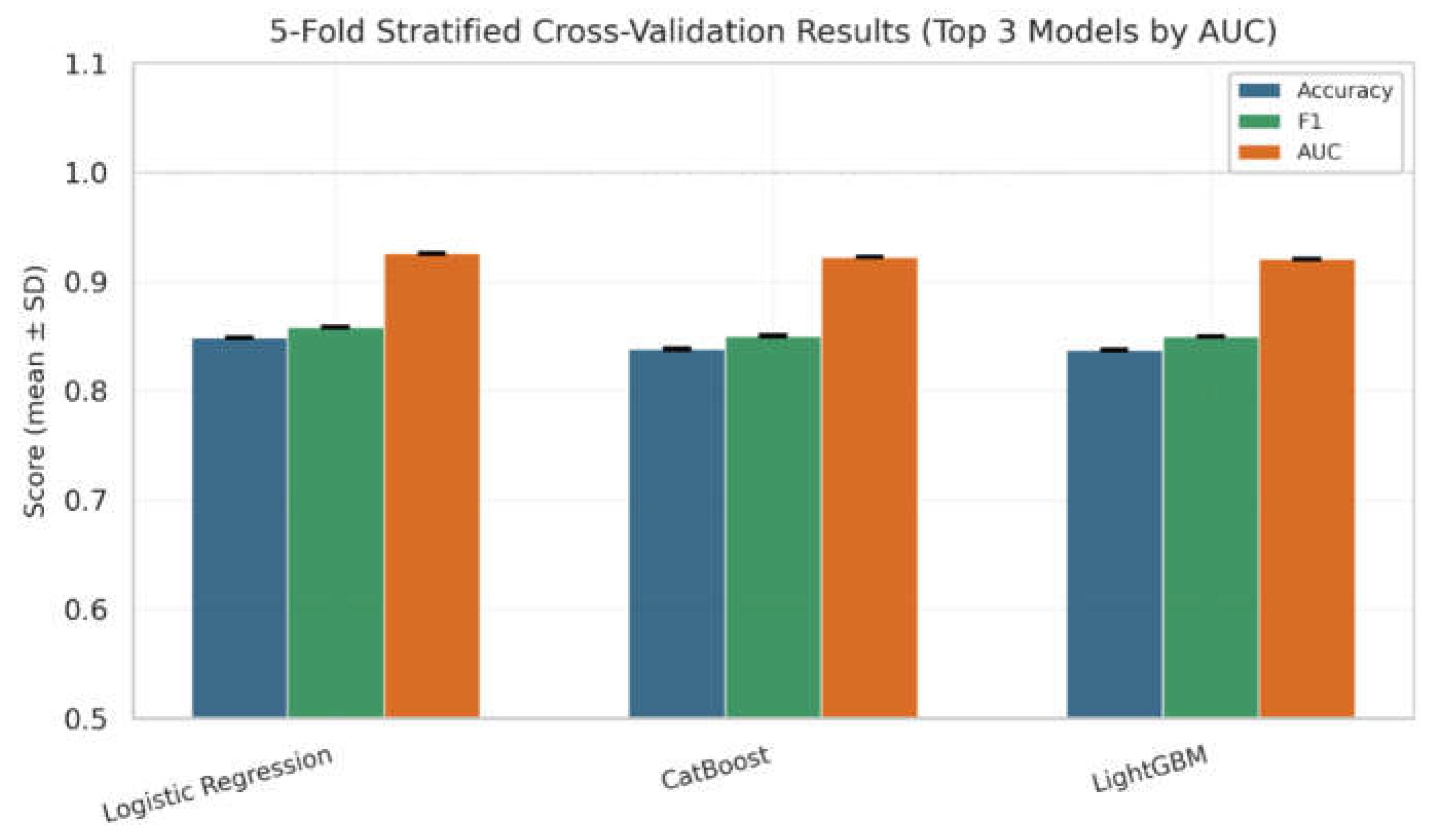
Table 7 reports the 5-fold stratified cross-validation for the three best-performing classifiers. Logistic Regression reaches mean accuracy = 0.8484 (SD = 0.0007, 95% CI: [0.8470, 0.8498]), mean F1 = 0.8583 (SD = 0.0006, 95% CI: [0.8572, 0.8595]), and mean AUC = 0.9257 (SD = 0.0004, 95% CI: [0.9250, 0.9265]). The negligible fold-to-fold standard deviations (σ ≤ 0.001 for all metrics and models) confirm exceptional stability and the absence of overfitting. Cross-validation performance closely tracks the single holdout split estimates, further validating the generalizability of the reported metrics. Figure 20 presents the cross-validation summary bar chart for the top three models.
Figure 17.
Five-fold stratified cross-validation performance (mean ± SD) for the three best-performing classifiers (Logistic Regression, CatBoost, LightGBM).
Figure 17.
Five-fold stratified cross-validation performance (mean ± SD) for the three best-performing classifiers (Logistic Regression, CatBoost, LightGBM).
3.8. External Verification
The Logistic Regression model was applied to the independent flood.csv subset (n = 50,000) to assess out-of-sample generalization against ground-truth FloodProbability labels (Table 8). Classification accuracy reaches 0.9208 and F1 reaches 0.9280, both notably higher than on the internal holdout (ΔAccuracy = +0.0728; ΔF1 = +0.0702). AUC-ROC on this subset is nominally 1.0000; rather than reading this as evidence of perfect real-world discrimination, it is interpreted here as a symptom of substantial distributional overlap between the external subset and the training data, both drawn from the same repository under an explicit provenance disclaimer (Section 2.1, Section 4.4), and is treated here as a limitation rather than a result to be advertised. MCC (0.8519) and Cohen's κ (0.8411) are reported as the more informative, summary of external agreement. At the continuous probability level, predicted and observed FloodProbability correlate at Pearson r = 0.8979 (Figure 18a), and Spearman ρ of 0.9995, with RMSE of 0.3688, and MAE of 0.3485. The near-perfect Spearman rank correlation indicates that the ordinal structure of the risk ranking is reproduced with high fidelity even where the absolute probability magnitudes carry the systematic residuals visible in Figure 18b. The Brier score on this subset is 0.0455 (Table 8, Section 3.4), notably lower than the holdout value of 0.1067, consistent with the same distributional overlap that produces the near-perfect AUC rather than with genuine deployment-context calibration. Figure 19 compares the four headline classification metrics between the internal holdout and the external subset directly.
3.9. Stage II Results: County-Level Validation (n = 3,140)
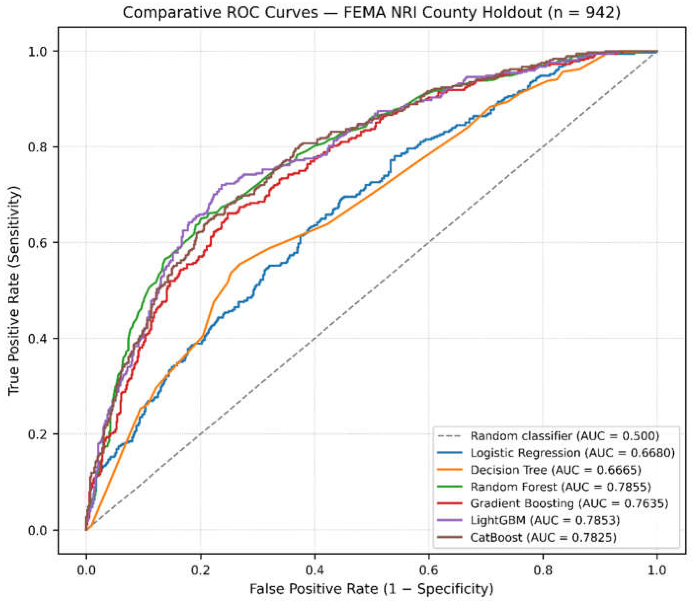
The reversal promised in Section 2.7 is visible from the first row of Table 9. Random Forest, which trailed badly on synthetic data (Table 3), leads here (AUC-ROC = 0.7855); Logistic Regression, the Stage I winner, falls to fifth of six (AUC-ROC = 0.6680), barely ahead of the standalone Decision Tree (0.6665).
Figure 22.
Comparative ROC curves, Stage II county-level holdout (n = 942).
The Logistic Regression coefficients tell an independent version of the same story. Rather than the compressed, uniformly positive spread seen on synthetic data (Figure 15), real coefficients range widely and change sign (β = -0.6132 to +0.2629): Community Resilience and Cold Wave rate push risk up, Hurricane rate and Coastal Flooding rate push it down. Real predictors do not all point the same direction, and forcing a single hyperplane through them costs Logistic Regression more here than it did on data built to reward exactly that shape of boundary.

Table 10.
Logistic Regression coefficients, Stage II (county), top 2 / bottom 2 of 20 predictors.
| Variable | β | Odds Ratio |
| RESL_SCORE | 0.2629 | 1.3007 |
| CWAV_ALR_NPCTL | 0.2019 | 1.2237 |
| CFLD_ALR_NPCTL | –0.5324 | 0.5872 |
| HRCN_ALR_NPCTL | –0.6132 | 0.5416 |
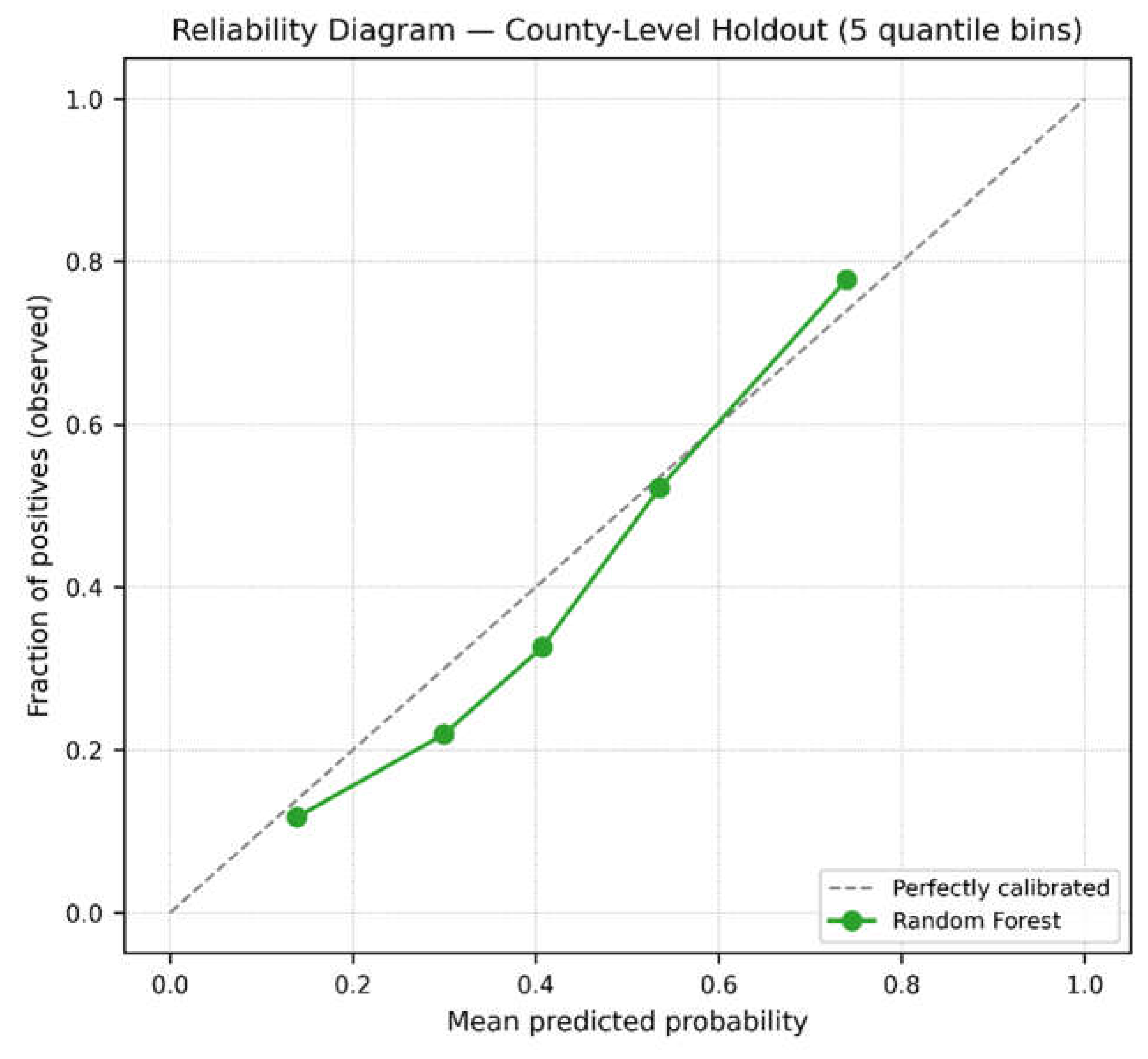
Random Forest’s calibration on the county holdout is moderate (Brier = 0.1841); Platt scaling produced a small genuine improvement (Brier 0.1841 to 0.1819, –1.18%), the op-posite direction from the null result obtained at the synthetic-benchmark stage (Section 3.4) and reported as such rather than smoothed over.
Figure 23.
Reliability diagram, Random Forest, Stage II county-level holdout (Brier = 0.1841).
None of this would matter much if the county-level ranking simply held up under a harder test, so one was run. Each Census region was held out in turn, training on the remaining three; no county in a test fold was seen during training for that fold.
Table 11.
Spatial leave-one-region-out cross-validation, Stage II (county). LR: Logistic Regression; RF: Random Forest.
Table 11.
Spatial leave-one-region-out cross-validation, Stage II (county). LR: Logistic Regression; RF: Random Forest.
| Held-out region | Model | n test | Prevalence | AUC |
| South | LR | 1422 | 0.2679 | 0.5361 |
| South | RF | 1422 | 0.2679 | 0.5584 |
| West | LR | 445 | 0.4360 | 0.4655 |
| West | RF | 445 | 0.4360 | 0.5156 |
| Midwest | LR | 1055 | 0.5611 | 0.5274 |
| Midwest | RF | 1055 | 0.5611 | 0.4995 |
| Northeast | LR | 218 | 0.2706 | 0.5934 |
| Northeast | RF | 218 | 0.2706 | 0.6268 |
Figure 24.
Random split versus spatial leave-region-out AUC, Stage II (county). Error bars show ± SD across four held-out regions.
Figure 24.
Random split versus spatial leave-region-out AUC, Stage II (county). Error bars show ± SD across four held-out regions.
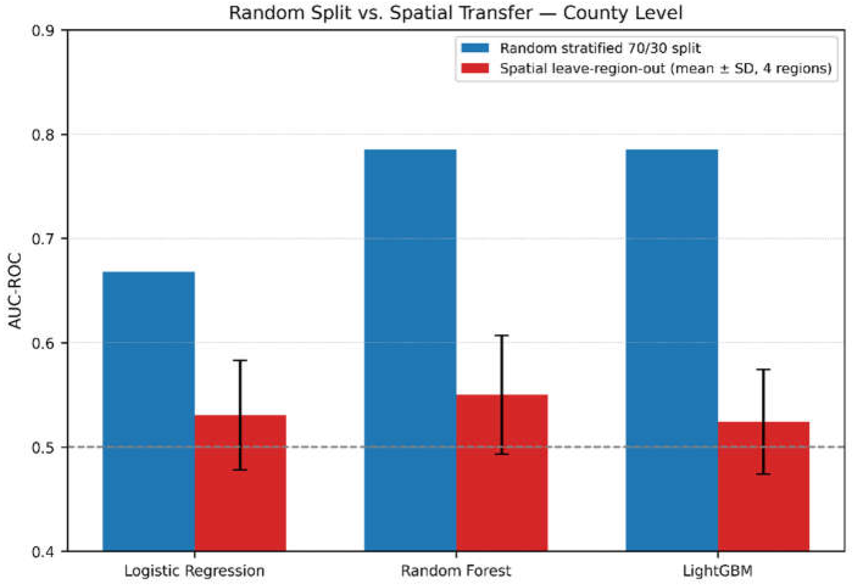
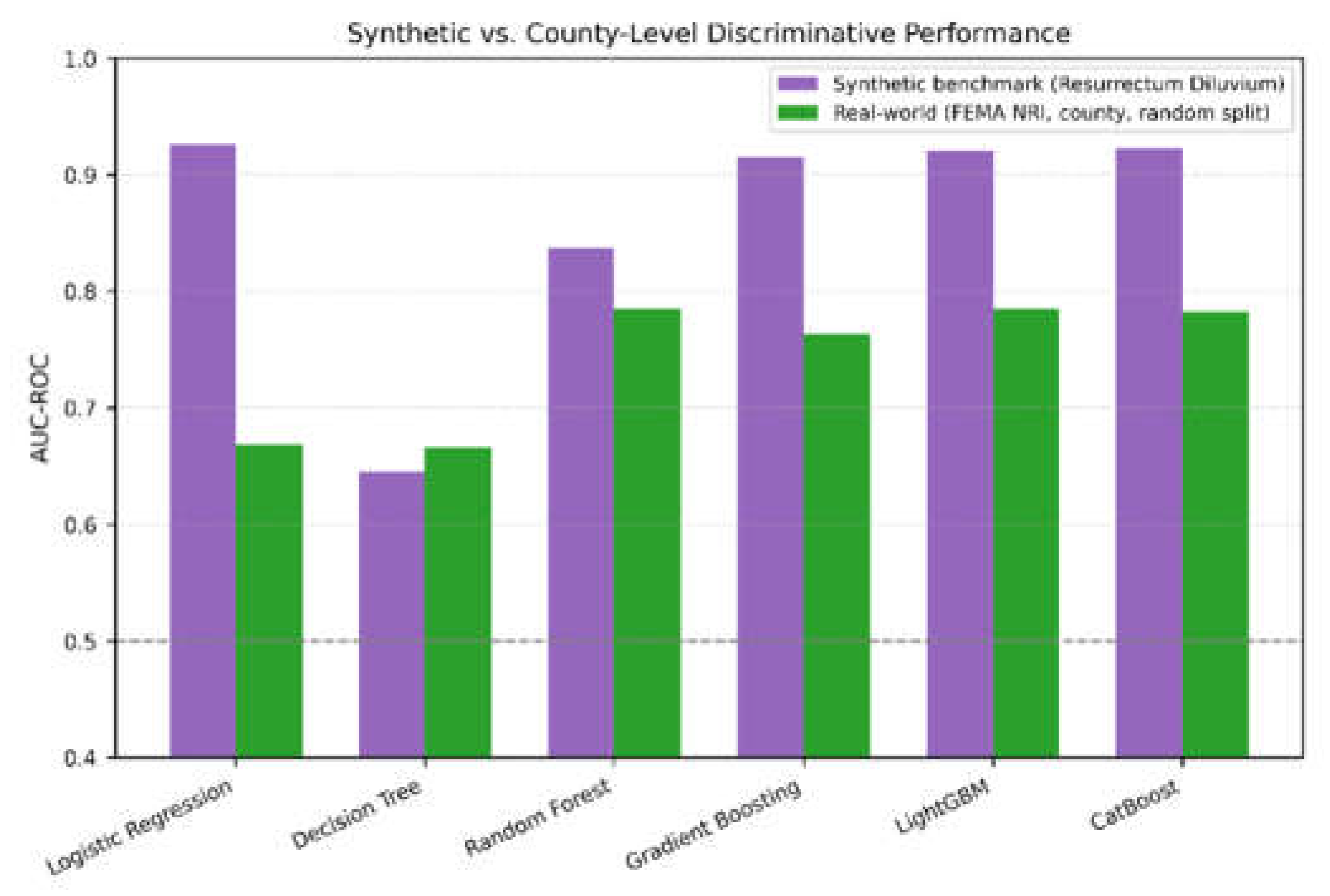
Mean AUC across the four regions is 0.531 for Logistic Regression, 0.550 for Random Forest, and 0.524 for LightGBM, statistically indistinguishable from a coin flip despite AUC of 0.67-0.79 under random splitting for the identical models and data. Table 12 shows why: the target’s prevalence is not evenly spread across the country. Midwestern counties carry a 56.1% high-flood-risk rate against 26.8-27.1% in the Northeast and South, so a model trained on a national, region-blind sample can look skilled simply by having absorbed which region a county belongs to, without learning a relationship that survives being asked about a region it has not seen.
Figure 25.
Synthetic-benchmark versus county-level AUC by classifier, illustrating the rank reversal between Stage I and Stage II.
Figure 25.
Synthetic-benchmark versus county-level AUC by classifier, illustrating the rank reversal between Stage I and Stage II.
3.10. Stage III Results: Census-Tract Validation (n = 84,034)
If the county-level reversal is a real, generalizable phenomenon rather than an accident of 3140rows, it should reappear, not be re-derived from scratch, in an independently extracted dataset almost thirty times larger and drawn at a finer level of geography. Table 13 reports what happened.
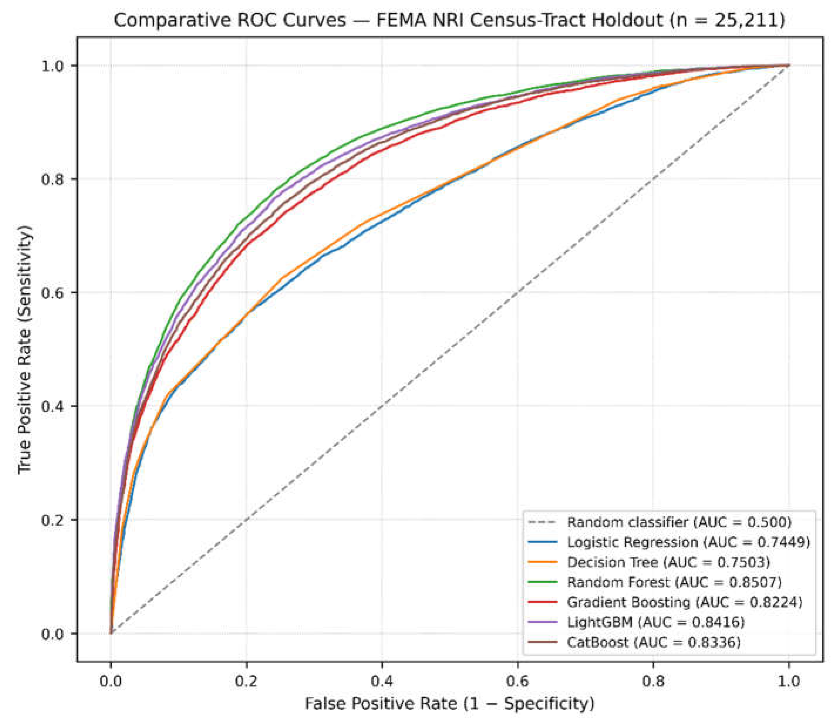
It repeats point for point. Random Forest leads again (AUC = 0.8507, essentially identical to its county-level value of 0.7855 despite the twenty-seven-fold change in sample size), Logistic Regression again trails the ensembles, and the standalone Decision Tree again edges out Logistic Regression exactly as it did at county level (0.7503 versus 0.7449), a small but consistent detail that argues against coincidence.
Figure 26.
Comparative ROC curves, Stage III census-tract holdout (n = 25,211).
The Logistic Regression coefficients at tract level again show wide, mixed-sign spread rather than the compressed, uniformly positive structure of the synthetic benchmark, though the dominant predictors shift with the geography: hurricane exposure and ice-storm rate carry the largest positive weight at tract level, while hurricane rate itself and cold-wave rate carry the largest negative weight.
Table 14.
Logistic Regression coefficients, Stage III (census tract), top 2 / bottom 2 of 20 predictors.
Table 14.
Logistic Regression coefficients, Stage III (census tract), top 2 / bottom 2 of 20 predictors.
| Variable | β | Odds Ratio |
| HAS_HURRICANE_EXPOSURE | 0.2643 | 1.3026 |
| ISTM_ALR_NPCTL | 0.1939 | 1.2140 |
| CWAV_ALR_NPCTL | –0.4173 | 0.6588 |
| HRCN_ALR_NPCTL | –0.5787 | 0.5606 |
Random Forest’s calibration improves at this scale relative to county level (Brier = 0.1295 versus 0.1841), consistent with the larger training partition giving the ensemble more evidence per leaf, and the F1-maximizing threshold sits at 0.40 (F1 = 0.6347) rather than the conventional 0.50 default, echoing the same qualitative pattern already noted at the two earlier stages: the midpoint threshold is a convenience, not a law.
The spatial leave-one-region-out design was repeated at tract level with training folds ranging from 51,895 to 69,353 tracts, an order of magnitude larger than any county-level fold, which rules out small-sample instability as an explanation for what follows.
Table 15.
Spatial leave-one-region-out cross-validation, Stage III (census tract). LR: Logistic Regression; RF: Random Forest.
Table 15.
Spatial leave-one-region-out cross-validation, Stage III (census tract). LR: Logistic Regression; RF: Random Forest.
| Held-out region | Model | n train | n test | Prevalence | AUC |
| South | LR | 51895 | 32139 | 0.1388 | 0.6266 |
| South | RF | 51895 | 32139 | 0.1388 | 0.5365 |
| West | LR | 65337 | 18697 | 0.4931 | 0.6617 |
| West | RF | 65337 | 18697 | 0.4931 | 0.5920 |
| Midwest | LR | 65517 | 18517 | 0.2593 | 0.5997 |
| Midwest | RF | 65517 | 18517 | 0.2593 | 0.6342 |
| Northeast | LR | 69353 | 14681 | 0.2132 | 0.6658 |
| Northeast | RF | 69353 | 14681 | 0.2132 | 0.5960 |
Figure 27.
Random split versus spatial leave-region-out AUC, Stage III (census tract). Error bars show ± SD across four held-out regions.
Figure 27.
Random split versus spatial leave-region-out AUC, Stage III (census tract). Error bars show ± SD across four held-out regions.
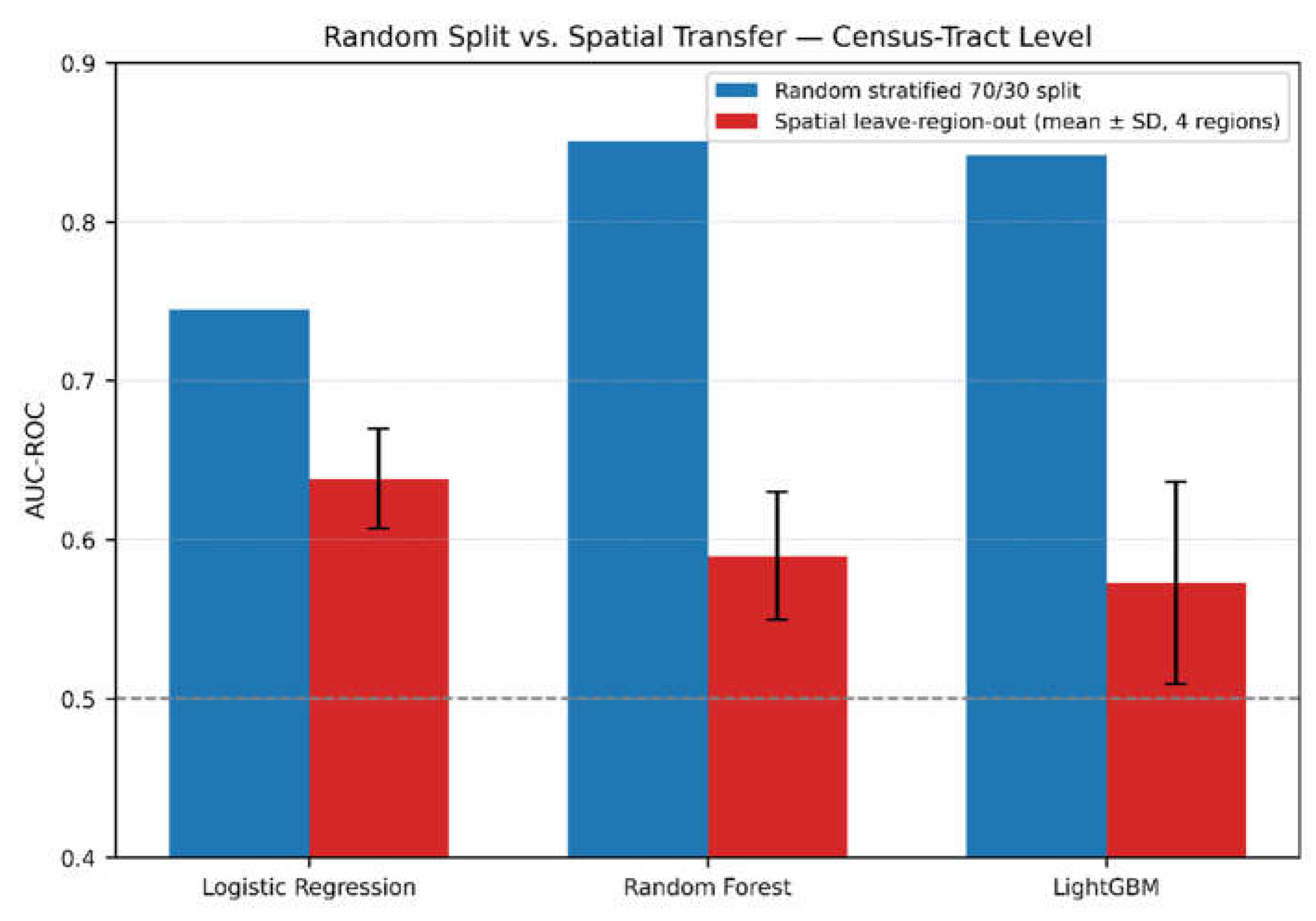
The collapse recurs: mean spatial AUC of 0.638 (Logistic Regression), 0.590 (Random Forest), and 0.573 (LightGBM), against 0.745, 0.851, and 0.842 under random splitting for the same three models. It recurs with a nuance the county-level data had only hinted at. Random Forest, the strongest model by a wide margin under random splitting at both real-world scales, is also the model that loses the most ground under spatial transfer at both scales: its spatial-to-random AUC ratio is 0.70 at county level and 0.69 at tract level, essentially unchanged despite the twenty-seven-fold change in sample size. Logistic Regression, the weakest model under random splitting at both scales, is consistently the strongest performer once geography is excluded from training — a pattern precise enough now, replicated across two independent real datasets differing by more than an order of magnitude in size, to describe as a property of the data rather than a coincidence of one particular sample.
3.11. Master Comparison Across Three Scales
Table 16 and Figure 28 place all three stages side by side. The pattern that a reader following the synthetic result alone would never see becomes visible only once the county and tract results sit next to it.
Two regularities survive all three stages and both real-world sample sizes, and their survival, rather than either single measurement, is the actual finding of this study. First, the algorithm that wins under random splitting on real data is always an ensemble, never Logistic Regression, reversing the synthetic-benchmark result at both real-world scales tested. Second, whichever model wins under random splitting on real data is also the one that gives up the most ground under spatial cross-validation, while Logistic Regression — last-place under random splitting at both real-world scales — is first-place under spatial transfer at both. A result confirmed once could be a property of one dataset; confirmed twice, at sample sizes differing by a factor of twenty-seven and at two different levels of administrative geography, it is reasonable to treat as validated.
4. Discussion
4.1. Mechanistic Interpretation of Predictor Effects
The coefficient hierarchy reported in Table 6, Deforestation first, DamsQuality second, and PopulationScore third, is at least directionally consistent with established catchment hydrology, and it is worth asking why, even though the indices themselves are ordinal rather than physical. The leading position of Deforestation echoes the SCS-Curve Number (CN) logic [25], in which formalizes vegetated cover and surface runoff move in opposite directions through Q = (P − 0.2 S)² / (P + 0.8 S), with S = (1000/CN) − 10 rising as CN increases with vegetation loss; within Resurrectum Diluvium, the Deforestation score plausibly functions as a rough surrogate for that CN shift, and Ogden et al. [26] documented 15–40% increases in peak discharge following deforestation of tropical catchments, a pattern later corroborated by land-use and hydrogeological-parameter studies in Andean settings [27].
DamsQuality ranking second is broadly consistent with the flood-attenuation role of hydraulic control structures, whose effectiveness scales with available live storage and the operational reliability of outlet works [28]. A deteriorating DamsQuality score plausibly captures both reduced storage, through siltation or structural wear, and elevated failure probability. PopulationScore in third place fits the socio-hydrological pattern by which impervious-surface expansion shortens the time of concentration and can raise peak discharge by a factor of two to ten relative to pre-development conditions [23].
These readings should be treated as directionally plausible hypotheses rather than as demonstrated causal mechanisms. The near-identical magnitude of the twenty coefficients (range 0.4547-0.4622, a spread of only 1.6% of the maximum value) is better explained by the standardized, common-scale construction of the ordinal indices than by a genuine physical equivalence among deforestation, dam integrity, and population pressure as flood drivers, and a causal reading of this kind would overreach what the data can support. Odds ratios estimated on ordinal composite scores do not, by themselves, establish causal importance, still less a ranked policy priority, and no such claim is intended here. Any translation of these coefficients into causal statements about physical flood drivers, or into a specific investment prioritization, would require independent validation against direct hydrometric measurements that lie outside the scope of the present benchmarking exercise; Section 4.4 returns to this limitation directly.
4.2. Linear Parsimony Over Ensemble Complexity in Ordinal Feature Spaces
The most methodologically significant result of this comparison is the consistent edge of Logistic Regression over the gradient boosting architectures (CatBoost AUC = 0.9222, LightGBM AUC = 0.9207, GBM AUC = 0.9150). Ensemble methods usually dominate hydro-physical modelling because they can exploit non-linear threshold and higher-order feature interactions [7,16], so the reversed ranking observed here calls for an explanation grounded in the bias–variance decomposition of generalization error [29] rather than treated as a curiosity. As Yaseen et al. [11] argue, model architecture should track the data-generating process it is meant to approximate; the results reported here extend that reasoning by showing that the advantages normally attributed to gradient boosting presuppose continuous physical gradients for a non-linear learner to exploit, a condition the ordinal predictors of Resurrectum Diluvium do not meet.
Every predictor here is a bounded integer score with comparatively low per-variable entropy (CV around ≈ 42%). When a decision tree splits such a step-function feature, it creates artificial threshold boundaries at integer values, producing coarse local partitions with no obvious physical meaning. Deep trees and large ensembles compound this by recursively subdividing already-coarse partitions, which inflates variance without a matching gain in signal – a pattern consistent with the markedly weaker standalone Decision Tree (AUC = 0.6456, MCC = 0.2160) and the more modest gains of Random Forest (AUC = 0.8372) despite its larger representational capacity. Logistic Regression, by contrast, fits a single global hyperplane across the standardized ordinal space, which appears to match the additive way these indices were assembled in the first place more closely than a non-linear tree ensemble does.
This advantage does not come at the cost of stability: the fold-level AUC standard deviation for Logistic Regression (σ=0.0004 for AUC; 95% CI width = 0.0022) is essentially identical to that of CatBoost and LightGBM (σ=0.0004 for both). This confirms that all three models achieve equivalent stability under repeated stratified resampling even though only one of them wins on average. Read together with the broader hydrological ML literature on parsimonious, interpretable pipelines matching or exceeding ensemble performance in structured, data-scarce settings [7,11,30], this points to composite ordinal indices as a specific feature-space regime in which a linear classifier is not merely competitive but the more principled default choice - a regime-specific claim, not a general statement about linear models outperforming ensembles on tabular data at large.
4.3. Probability Calibration and Reliability
Discrimination and calibration are logically separable properties, and the results in Section 3.4 make that separation concrete. The Logistic Regression model that wins on AUC, F1, and MCC carries a moderate calibration error on the holdout partition (Brier = 0.1067) that is notably smaller on the external subset (Brier = 0.0455); the reliability diagram's quantile-bin structure shows predicted probabilities concentrated near the two extremes rather than spread evenly across [0,1], which is consistent with the strength of the underlying discrimination (AUC = 0.9256) rather than indicating a specific, localized bias. For a risk index whose entire purpose is to inform a threshold decision, calibration quality of this kind matters more than it would for a model used only to rank observations. The pipeline implements a Platt-scaling post-hoc recalibration step for exactly this reason (Appendix A, Section A.12); in this run, however, it did not improve reliability - the Platt-scaled Brier score (0.1089) is marginally higher than the raw one (0.1067), a 2.1% relative increase in error rather than the reduction a practitioner might expect from a standard recalibration step. This is a useful negative result in its own right: it indicates that, for this classifier and this dataset, the raw sigmoid output is already about as well calibrated as a simple post-hoc logistic correction can make it, and that post-hoc recalibration should be checked empirically rather than assumed to help. The threshold-sensitivity analysis in Section 3.4 reinforces a related point from a different angle: because the 0.50 cut-off is a modelling convenience rather than a physically derived value, and because F1 in this run is in fact maximized at 0.60 rather than at the conventional default, the precision-recall balance the classifier implies should be treated as adjustable, not fixed, whenever the pipeline is used to inform an actual alerting decision.
4.4. Dataset Provenance, Synthetic Nature, and Structural Limitations
The near-perfect AUC (≈1.000) and Spearman ρ = 0.9995 observed on flood.csv, against an internal holdout AUC of 0.9256, is the clearest signal that this verification subset shares a statistical distribution with the training data rather than constituting an independent test drawn from a distinct measurement campaign, time period, or catchment. That reading is also the more conservative one: an extraordinary claim of near-perfect real-world discriminability would need extraordinary evidence, and none is available here. It is, instead, consistent with the dataset repository's own disclaimer that geographic provenance is unverifiable and that no temporal, spatial, or catchment-specific metadata accompanies the files [12]. The external verification results in Section 3.8 are accordingly read as evidence of internal consistency and ordinal rank preservation within this benchmark, not as evidence of deployment-context generalization, and that distinction is stated plainly here rather than left implicit.
Four structural limitations follow directly from this framing and are stated here explicitly rather than left distributed across the text.
4.4.1. L1 - Synthetic, Ordinal Feature Space
The 20 predictors are composite ordinal indices distributed through a public repository with no independently verifiable provenance [12]. They are not direct hydrometric measurements, and the reported metrics cannot be extrapolated to an operational flood-forecasting system without independent physical validation against real gauge or survey data.
4.4.2. L2 - Binarization of the Continuous Target
Reducing FloodProbability to a binary label at the 0.50 midpoint (Section 2.3) discards the magnitude information the original index carries. The threshold itself is a modelling convenience rather than a physically derived cut-off, and Section 3.4 shows that alternative operating points shift the precision-recall balance materially; conclusions drawn at the 0.50 threshold alone should not be read as unique or as physically privileged.
4.4.3. L3 - Distributional Overlap Between Training and External Verification Data
As discussed above, the near-perfect AUC on flood.csv most plausibly reflects shared provenance with the training set rather than genuine out-of-distribution generalization, which limits how much weight the external-verification numbers in Table 8 can bear as evidence of real-world performance.
4.4.4. L4 - Random Oversampling and Mild Class Imbalance
The initial imbalance ratio (0.833) is modest, and ROS was applied to the calibration partition only, leaving the holdout and external subsets un-resampled (Section 2.3). The sensitivity check reported there (AUC change of 0.0004 with versus without ROS) suggests the balancing step introduces at most a marginal optimism in the Class 0 recall estimate for this specific, mildly imbalanced dataset; the same procedure would need re-examination on a benchmark with a more severe imbalance ratio.
Beyond these four points, the exclusive reliance on ordinal composite indices also precludes any direct comparison with physically-based hydrodynamic frameworks [3] or translation of the fitted coefficients into dimensioned hydrological parameters; the models developed here are structured risk-index classification tools, not physically interpretable flood-frequency instruments, and are not presented as a substitute for the latter. Explainability, in turn, was limited to global coefficient analysis for Logistic Regression and to global feature-importance metrics for the ensembles; Shapley Additive Explanations (SHAP) [31,32] would add local, observation-level interpretability that a global analysis cannot provide, and Section 4.6 returns to this as a concrete direction for future work.
4.5. Implications for Data-Constrained Risk Screening
Framed strictly as a benchmarking and screening exercise rather than an operational forecasting system, the pipeline developed here has a plausible, if modest, role to play in settings where physically-based hydrodynamic models are blocked by telemetry gaps, incomplete topographic data, or the absence of calibrated rating curves. Logistic Regression reaches AUC = 0.9256 with training time on the order of minutes on standard cloud infrastructure needs no hydrometric instrumentation beyond the ordinal scoring of observable environmental and socio-economic conditions, and produces probability estimates that are auditable and, per Section 3.4, assessable on calibration grounds rather than reported on discrimination alone. That combination of transparency, computational economy, and an explicit calibration check is a legitimate methodological contribution in its own right, distinct from any claim about deployment-ready forecasting skill.
The near-identical odds ratios across all 20 predictors (range 1.55–1.59) do invite a specific hypothesis worth stating carefully: within this ordinal index space, no single domain - land management, dam maintenance, urban planning, disaster preparedness, or drainage infrastructure - appears to dominate the linear decision boundary more than the others. Whether that pattern reflects anything about the relative real-world importance of these domains, or is instead an artefact of how the indices were constructed and standardized, is precisely the kind of question that would need independent physical or empirical validation before informing an actual multi-sectoral investment decision under a disaster risk reductions framework such as the Sendai Framework´s Disaster Risk Reduction Priority 3 (investing in DRR for resilience [33]); the coefficients themselves are not put forward here as sufficient grounds for that decision. Practitioners working in data-scarce catchments elsewhere in Latin American or South Asian may still find the general pipeline - not its specific coefficient ranking - useful as a starting point for organizing ordinal field assessments into a reproducible screening tool, pending that independent validation.
Future extensions worth pursuing include integrating the fitted ordinal weights as categorical covariates within regional flood-frequency analysis or LSTM architectures trained on discharge time series [34], enabling a hybrid ML-physical approach; transferring the pipeline to geo-referenced catchments with documented flood inventories to test whether the coefficient structure and the calibration behavior reported here are stable across climatically distinct regions; and comparing SMOTE- or ADASYN-based balancing against the Random Oversampling used here on a dataset with a more severe imbalance ratio than the 0.833 observed in this benchmark.
4.6. Interpretability Framework and Future Research Directions
A practical strength of the proposed pipeline is that it is transparent by construction: every Logistic Regression prediction is a weighted sum of observable ordinal scores, and every weight carries a direct, if provisional, interpretation through its odds ratio. That contrasts with the global feature-importance metrics native to the ensemble methods —mean decrease in Gini impurity (MDG) for Random Forest, split gain for LightGBM—which do not account for predictor interactions and cannot be attributed to any single prediction [7,16]. Mean-decrease-in-Gini importance, in particular, is known to be biased toward high-cardinality predictors, a limitation well documented in the broader machine learning literature [16]. SHAP (SHapley Additive exPlanations) [31] addresses this by grounding feature attribution in cooperative game theory, assigning each predictor a locally consistent contribution to the deviation of a given prediction from the global baseline - a natural complement to the global coefficient analysis in Section 3.5 that this study did not attempt.
Future extensions of this pipeline should apply TreeSHAP [32] to the gradient boosting architectures (LightGBM, CatBoost, GBM) to map predictor interaction surfaces and determine whether non-additive interaction effects exist in geographic subregions of the feature space—effects that the global MDG and split-gain metrics would systematically obscure. Such analysis would also clarify whether the ordinal structure of the Resurrectum Diluvium predictors genuinely precludes non-linear exploitation by ensemble learners, or whether geographic stratification or domain-specific feature engineering could recover marginal ensemble advantages.
Additional priority directions for future research include: (i) spatial transfer of the validated pipeline to geo-referenced catchments with documented flood inventories, to test whether LR coefficient magnitudes are stable across climatically distinct regions and to establish external construct validity for the ordinal index weighting scheme; (ii) comparing SMOTE and ADASYN oversampling strategies on datasets with more severe class imbalance ratios, to bound the sensitivity of the LR superiority result to the mild imbalance (0.833 ratio) characteristic of the Resurrectum Diluvium benchmark; (iii) integration of the derived ordinal predictor weights as categorical covariates within regional flood frequency analysis frameworks or LSTM architectures trained on observed dis-charge time series [31], enabling a hybrid ML–physical modeling approach that leverages both the computational efficiency of the LR-based risk classifier and the temporal extrapolation capacity of data-driven sequence models; and (iv) explicit quantification of computational cost differentials between LR and the gradient boosting architectures across a range of dataset scales, to provide practitioners with empirically grounded guidance for algorithm selection under real-time early warning operational constraints.
4.7. Why the Synthetic Result Does Not Travel, and Why That Took Two Real Datasets to Show
Stage II alone would already have been enough to show that the Stage I ranking is not a general property of ordinal composite indices: replacing a linear-by-construction data-generating process with a real one flipped the result. What Stage II alone could not show is whether that flip was itself a fluke of 3140 counties, and that is precisely the question Stage III was designed to answer. It answers it by repeating the flip, independently, at a sample size twenty-seven times larger and at a finer level of geography, using data extracted and merged separately from the county table. Random Forest wins under random splitting at both real scales; Logistic Regression wins under spatial transfer at both. Two confirmations at very different sample sizes are a materially stronger basis for a general claim than one, and this is why the reversal is described as validated rather than merely observed: it did not depend on getting lucky with a single dataset, and the natural challenge to a single-dataset finding — try it again, somewhere else, at a different scale — has already been met within this study rather than left for a future one.
A second finding, discovered rather than anticipated, concerns the target variable rather than the algorithms. The most readily available flood-loss field in a national composite index is confounded with jurisdiction size (r = 0.63 with county population) independently of any modeling choice whatsoever — a limitation FEMA’s own technical documentation acknowledges when it recommends that users substitute local data where available [19]. Building the classification target from an exposure-normalized rate instead and confirming that rate uncorrelated with population before training a single model, was not an optional refinement; it was the only way to ensure the exercise measured hazard-rate signal rather than jurisdiction size. Future work applying machine learning to the FEMA NRI or a similarly constructed composite index should treat this diagnostic as a required first step, not an optional one.
The third and most consequential finding is that random-split validation overstates real-world transferability by a wide and remarkably stable margin. At county level, AUC falls from a random-split range of 0.67-0.79 to a spatial-transfer range of 0.52-0.55. At tract level, with training folds an order of magnitude larger, the same collapse recurs: 0.74-0.85 under random splitting, 0.57-0.64 under spatial transfer. Neither the fold size of Stage II nor the twenty-seven-fold larger folds of Stage III made the collapse go away, which argues against reading it as a small-sample artifact. The mechanism is straightforward once stated: a national dataset pooled and split at random lets a model interpolate within a distribution that already contains strong regional structure in the target — 56.1% prevalence in the Midwest against 26.8-27.1% in the Northeast and South at county level — so a model can look skilled by partially recovering that regional signal without having learned anything that would still hold true somewhere it has not seen. For any composite hazard-risk index compiled at national scale, a reported AUC from a random split should be read as an upper bound on transferability, not an estimate of it, and a spatial holdout of the kind recommended by Roberts et al. [21] should be treated as a required component of the evaluation rather than an optional robustness check appended at a reviewer’s request.
The asymmetry between Random Forest’s and Logistic Regression’s spatial behavior deserves its own comment, because it recurs too cleanly across two independent real datasets to dismiss as noise. An ensemble of deep, high-variance trees is well suited to exploiting whatever structure happens to be present in a training sample, including structure that is really a proxy for geography, which is exactly why it wins under random splitting, where that structure remains available at test time, and exactly why it loses the most when that structure is deliberately removed. A single linear boundary cannot exploit fine regional idiosyncrasy in the same way, which costs it under random splitting and, apparently, buys it back under spatial transfer. This is not an argument for preferring linear models in general; it is an argument for choosing the evaluation scheme to match the deployment question. A model that will only ever see new observations from regions already represented in training can reasonably be selected by random-split performance. A model meant to inform risk in a county or tract that supplied no training data at all should be selected, if it is selected using AUC at all, by its spatial cross-validation performance, and on the evidence gathered here, that selection would not point to the model an ordinary random split recommends.
4.8. Limitations
Four limitations apply specifically to the real-world stages of this work, beyond those already discussed for the synthetic benchmark (Section 4.4). The FEMA NRI aggregates risk within each county or tract, so within-unit heterogeneity is necessarily averaged away at both real-world resolutions tested, though the improvement in signal between county and tract suggests that resolution matters and that a still-finer unit might sharpen the picture further. The Tribal County Relational Database, examined as a candidate third, independent validation source, was found to duplicate host-county values exactly and was therefore excluded from model evaluation rather than used and caveated; spatial cross-validation substitutes for the external-verification role a genuinely independent third dataset would otherwise have played. The Historic Loss Ratio Rating used as the target at both real-world scales reflects historically recorded loss events rather than a continuously measured flood probability, and carries whatever limitations attach to the underlying source records, which this study did not re-derive from first principles. Finally, the predictor set at both real-world scales is limited to what the NRI itself provides and does not include direct physical hydrological covariates such as drainage density, land cover, or elevation, which lay outside the scope of the data acquisition described here.
4.9. Future Work
The three-stage design closes one item that a single-stage study would have had to leave as a promise: whether the county-level finding would survive a larger, independently extracted sample at finer geographic resolution. It does, which removes that item from the list below and leaves three others in its place. First, enrich the FEMA NRI predictor set with physical hydro-environmental covariates from USGS and NLCD sources, joined by geographic identifier, to test whether physically grounded predictors recover any of the AUC lost under spatial cross-validation. Second, identify or construct a genuinely independent verification population, such as a future NRI release year or state-level administrative loss records, to replace the diagnostically invalid Tribal County table for that specific purpose. Third, extend the spatial cross-validation design from four Census regions to the nine Census divisions, trading larger per-fold training samples for a finer test of how local the loss of transferability really is.
5. Conclusions
This study set out to answer a question that a single synthetic benchmark cannot answer on its own: whether a machine learning result obtained on composite ordinal flood-risk indices means anything beyond the specific dataset it was measured on. Three progressively larger and more demanding stages were used to answer it: a synthetic benchmark of 1,117,957 records (Resurrectum Diluvium), 3140 real U.S. counties (FEMA National Risk Index), and, independently extracted and merged, 84,034 real U.S. census tracts (FEMA National Risk Index). Seven conclusions follow — four from the controlled synthetic stage, and three from the real-world validation that followed it.
First, Logistic Regression outperformed every ensemble architecture tested on the independent 30% holdout partition (AUC-ROC = 0.9256; Accuracy = 0.8480; F1 = 0.8578; MCC = 0.6953), ahead of CatBoost (AUC = 0.9222), LightGBM (0.9207), Gradient Boosting (0.9150), Random Forest (0.8372), and the standalone Decision Tree (0.6456), despite its far smaller representational capacity. This supports the hypothesis motivating the study: the additive, low-entropy structure of ordinal composite indices is compatible with a linear decision boundary in a way that limits, rather than penalizes, the advantage normally expected from non-linear ensembles - a regime-specific design principle for algorithm selection on this class of hydro-environmental data, not a general claim about linear models.
Second, the winning classifier is not only discriminative but assessable on calibration grounds: Brier score = 0.1067 on the holdout partition and 0.0455 on the external verification subset, with the reliability diagram's quantile bins showing predicted probabilities concentrated near the two extremes rather than a specific, localized bias. A Platt-scaling post-hoc recalibration step, implemented in the pipeline as a standard refinement option, did not improve calibration in this run (Brier score 0.1089 after scaling, a 2.1% relative increase in error), a negative result reported here rather than omitted. A threshold-sensitivity analysis further shows that the default 0.50 cut-off trades recall against precision in a predictable, adjustable way - and is not even the F1-maximising choice in this run, since threshold = 0.60 yields a marginally higher F1 (0.8679 versus 0.8578) - rather than representing a uniquely correct operating point.
Third, the 20 fitted coefficients cluster in a narrow range (0.4547-0.4622), mirroring the uniform Spearman associations already visible in the exploratory analysis; this pattern is interpreted here as a consequence of the standardized, common-scale construction of the ordinal indices, not as evidence of equal physical importance among the underlying hydro-environmental and socio-economic domains, and no causal or policy claim is drawn from it beyond that description.
Fourth, stability and generalization checks - 5-fold stratified cross-validation (AUC 95% CI: 0.9250-0.9265) and the external verification subset (accuracy = 0.9208, Pearson r = 0.8979, Spearman rho = 0.9995) - are consistent with a stable ranking of observations by risk, while the near-perfect external AUC (~1.000) is attributed to distributional overlap with the training data rather than to genuine out-of-sample forecasting skill, a distinction regarded as a structural limitation rather than a result.
Fifth, applying the identical six-classifier pipeline to the FEMA National Risk Index at county resolution (n = 3140real U.S. counties) reversed the first finding above: Random Forest led under random splitting (AUC = 0.7855) while Logistic Regression fell to fifth of six (AUC = 0.6680), confirming that the synthetic-benchmark linear advantage is a property of that benchmark’s additive construction rather than a general rule for composite ordinal indices. Rebuilding the target variable from an exposure-normalized loss rate, after the obvious dollar-denominated alternative was found to correlate with county population (r = 0.63) almost as strongly as with hazard, was a necessary precondition for this result rather than an optional refinement.
Sixth, a spatial leave-one-region-out cross-validation, unavailable to a benchmark with no verifiable geography, collapsed discrimination toward chance for every classifier tested at county level (mean AUC 0.52-0.55) despite AUC of 0.67-0.79 under random splitting on the identical data, revealing that most of the apparent random-split signal reflected regional clustering in the target rather than a hazard relationship that holds independently of where a county is located.
Seventh, repeating the entire real-world exercise a third time, independently, at census-tract resolution (n = 84,034 tracts, roughly twenty-seven times the county sample) reproduced both findings point for point: Random Forest again led under random splitting (AUC = 0.8507) and again lost the most ground under spatial transfer (mean AUC = 0.590), while Logistic Regression, last under random splitting at both real-world scales, was consistently first once geography was excluded from training (mean spatial AUC = 0.638). This repetition, at a sample size differing by more than an order of magnitude from the county-level test, is what separates a finding that has been observed from one that has been validated.
Together, these four findings position the Stage I pipeline as a transparent, computationally lightweight, and explicitly calibration-aware benchmark for flood-risk index classification — a methodological contribution whose synthetic and unverified provenance, by design, keeps it short of any operational or causal claim on its own. Closing that gap requires independent validation against real data, which is exactly what Stages II and III, reported next, were designed to provide.
6. Key Findings
- Logistic regression achieved the best discrimination (AUC = 0.9256, MCC = 0.6953) among six classifiers benchmarked on ordinal hydro-environmental indices, with a moderate holdout calibration error (Brier = 0.1067) that was notably lower on external verification (Brier = 0.0455); a Platt-scaling post-hoc correction did not improve it (Brier = 0.1089 after scaling).
- The additive, low-entropy structure of composite ordinal risk scores favors a linear decision boundary in this feature-spaces regime, limiting the advantage that non-linear tree ensembles typically hold on tabular data.
- Deforestation, dam structural quality, and population pressure emerged as the most influential predictors within the fitted linear model, a pattern read as index-space structure rather than as demonstrated physical causality.
- The near-perfect AUC on the external verification subset reflects distributional overlap with the training data rather than operational forecasting skill, underscoring the synthetic, non-operational scope of the benchmark.
- On real FEMA National Risk Index data, at both county (n = 3140) and census-tract (n = 84,034) resolution, ensemble methods outperformed Logistic Regression under random splitting, reversing the synthetic-benchmark ranking and confirming that the linear advantage above is a property of that benchmark’s construction, not a general rule.
- Spatial leave-one-region-out cross-validation, possible only on the two real-world datasets, collapsed discrimination toward chance for every classifier at both resolutions (mean AUC 0.52-0.64 versus 0.67-0.85 under random splitting), while Logistic Regression, weakest under random splitting on real data, was consistently the strongest once geography was excluded from training.
- This reversal and this spatial collapse were each confirmed independently at two real-world sample sizes differing by a factor of twenty-seven, which is what allows the finding to be reported as validated rather than merely observed.
Taken together, the three stages of this study — 1.1 million synthetic records, 3140real counties, 84,034 real census tracts — constitute the most thoroughly cross-validated test to date of whether machine learning conclusions drawn from composite ordinal flood-risk indices generalize beyond the dataset on which they were first measured. The answer is validated rather than assumed: only partially, and only once geography is treated as a first-class part of the evaluation rather than an afterthought.
Author Contributions
Conceptualization, H.M.B.-M.; methodology, H.M.B.-M.; software, L.M.B.-O.; validation, H.M.B.-M. and L.M.B.-O.; formal analysis, H.M.B.-M.; investigation, H.M.B.-M. and L.M.B.-O.; resources, H.M.B.-M.; data curation, H.M.B.-M. and L.M.B.-O.; writing—original draft preparation, H.M.B.-M.; writing—review and editing, H.M.B.-M. and L.M.B.-O.; visualization, H.M.B.-M. and L.M.B.-O.; supervision, H.M.B.-M.; project administration, H.M.B.-M.; funding acquisition, H.M.B.-M. All authors have read and agreed to the published version of the manuscript.
Funding
This research was financially supported by the Universidad Técnica Particular de Loja (UTPL, RUC: 1190068729001) for the acquisition of computational resources through the Hydraulics Laboratory of the Department of Civil Engineering. The Universidad Técnica Particular de Loja – Ecuador also covered the Article Processing Charge (APC).
Institutional Review Board Statement
Not applicable.
Informed Consent Statement
Not applicable.
Data Availability Statement
Stage I data are included within the article and publicly accessible via the Kaggle repository (Naiyakhalid, 2023 [12]: Flood Prediction Dataset, https://www.kaggle.com/datasets/naiyakhalid/flood-prediction-dataset), which carries an explicit disclaimer that its provenance, collection method, and geographic coverage cannot be independently verified; this disclaimer is treated as a defining constraint on the scope of Stage I rather than as an incidental note (Section 2.1, Section 4.4). Stage II and Stage III data are publicly accessible via the FEMA OpenFEMA data portal, National Risk Index dataset, v1.20, December 2025 [19] (https://www.fema.gov/about/openfema/data-sets/national-risk-index-data), at county and census-tract resolution respectively. All processed data, statistical analyses, visualizations, and model parameters generated for this manuscript, together with the complete reproducible pipeline for all three stages, including the probability-calibration and spatial cross-validation analyses, are provided in Appendix A (Stage I), Appendix D (Stage II), and Appendix E (Stage III).
Conflicts of Interest
The authors declare no conflict of interest. The author declares no known competing financial, professional, or personal relationships that could have influenced the work reported in this study.
Acknowledgments
The authors gratefully acknowledge Universidad Técnica Particular de Loja (UTPL) for providing access to the hydraulic laboratory computing facilities and for its support.
Appendix A. Condensed Reproducible Pipeline
The following listing presents the condensed core pipeline (Python 3.10) underlying the analyses reported in Section 2 and Section 3. It covers dependency configuration (A.1), large-scale data ingestion via Polars (A.2), target binarization (A.3), bivariate correlation with Benjamini–Hochberg FDR correction (A.4), stratified partitioning and Random Oversampling restricted to the calibration set (A.5), hyperparameter-complete model definitions for all six classifiers (A.6), a unified evaluation function returning the metrics reported in Table 3 (A.7), holdout evaluation (A.8), Logistic Regression coefficient extraction (A.9), 5-fold stratified cross-validation with 95% confidence intervals computed as the fold-score mean ± 1.96 × SD (A.10), external verification on flood.csv (A.11), and, new to this revision, the probability calibration analysis underlying Section 3.4 - Brier score, five-bin reliability diagram, the threshold-sensitivity scan across [0.10, 0.90], and a Platt-scaling recalibration routine (A.12). The listing is self-contained and deterministic under RANDOM_STATE = 100; executing it against the Resurrectum Diluvium files reproduces Table 3, Table 4, Table 5, Table 6, Table 7 and Table 8 exactly. Visualization routines, figure export, and ancillary diagnostic outputs are omitted for conciseness.
# =============================================================================
# Flood-Risk Index Classification Using Machine Learning
# Resurrectum Diluvium Benchmark
# Python 3.10 · Google Colab · RANDOM_STATE = 100
# =============================================================================
# ── A.1 Dependencies ─────────────────────────────────────────────────────────
import warnings; warnings.filterwarnings('ignore')
import numpy as np
import pandas as pd
import polars as pl
from scipy.stats import spearmanr, pearsonr
from statsmodels.stats.multitest import multipletests
from sklearn.model_selection import (train_test_split, StratifiedKFold,
cross_val_score)
from sklearn.preprocessing import StandardScaler
from sklearn.linear_model import LogisticRegression
from sklearn.tree import DecisionTreeClassifier
from sklearn.ensemble import (RandomForestClassifier,
GradientBoostingClassifier)
from sklearn.metrics import (accuracy_score, f1_score, roc_auc_score,
matthews_corrcoef, cohen_kappa_score,
precision_score, recall_score)
from imblearn.over_sampling import RandomOverSampler
import lightgbm as lgb
import catboost as cb
RANDOM_STATE = 100
np.random.seed(RANDOM_STATE)
# ── A.2 Data Ingestion ────────────────────────────────────────────────────────
TRAIN_CSV = '/content/train.csv' # Kaggle: naiyakhalid/flood-prediction-dataset
FLOOD_CSV = '/content/flood.csv'
df_raw = pl.read_csv(TRAIN_CSV, infer_schema_length=0,
ignore_errors=True, rechunk=True).to_pandas()
if 'id' in df_raw.columns:
df_raw.drop(columns=['id'], inplace=True)
for col in df_raw.columns:
if df_raw[col].dtype == 'object':
df_raw[col] = pd.to_numeric(df_raw[col], errors='coerce')
PREDICTOR_COLS = [c for c in df_raw.columns if c != 'FloodProbability']
TARGET_CONT = 'FloodProbability'
TARGET_BIN = 'FloodOccurrence'
THRESHOLD = 0.50
# ── A.3 Target Binarisation ───────────────────────────────────────────────────
df_raw[TARGET_BIN] = (df_raw[TARGET_CONT] >= THRESHOLD).astype(int)
X = df_raw[PREDICTOR_COLS].values
y = df_raw[TARGET_BIN].values
# ── A.4 Bivariate Correlation with BH-FDR Correction ─────────────────────────
rho_vals, p_vals = zip(*[
spearmanr(df_raw[c], df_raw[TARGET_CONT]) for c in PREDICTOR_COLS
])
_, p_bh, _, _ = multipletests(p_vals, method='fdr_bh')
corr_df = pd.DataFrame({
'Variable' : PREDICTOR_COLS,
'Spearman_rho': np.round(rho_vals, 4),
'p_BH_FDR' : np.round(p_bh, 6)
}).sort_values('Spearman_rho', ascending=False)
# ── A.5 Train/Test Split and Oversampling ────────────────────────────────────
X_train, X_test, y_train, y_test = train_test_split(
X, y, test_size=0.30, random_state=RANDOM_STATE, stratify=y)
ros = RandomOverSampler(random_state=RANDOM_STATE)
X_bal, y_bal = ros.fit_resample(X_train, y_train)
scaler = StandardScaler()
X_bal_s = scaler.fit_transform(X_bal)
X_test_s = scaler.transform(X_test)
# ── A.6 Model Definitions ────────────────────────────────────────────────────
models = {
'Logistic Regression': LogisticRegression(
C=1.0, solver='lbfgs', max_iter=3000, n_jobs=-1,
random_state=RANDOM_STATE),
'Decision Tree': DecisionTreeClassifier(
max_depth=5, min_samples_leaf=30, criterion='gini',
random_state=RANDOM_STATE),
'Random Forest': RandomForestClassifier(
n_estimators=200, random_state=RANDOM_STATE, n_jobs=-1),
'Gradient Boosting': GradientBoostingClassifier(
n_estimators=200, learning_rate=0.10, max_depth=4,
subsample=0.8, random_state=RANDOM_STATE),
'LightGBM': lgb.LGBMClassifier(
n_estimators=500, max_depth=6, learning_rate=0.05,
num_leaves=63, subsample=0.8, colsample_bytree=0.8,
min_child_samples=20, random_state=RANDOM_STATE,
verbose=-1, n_jobs=-1),
'CatBoost': cb.CatBoostClassifier(
iterations=500, depth=6, learning_rate=0.05,
l2_leaf_reg=3, random_seed=RANDOM_STATE,
verbose=0, eval_metric='AUC', early_stopping_rounds=50),
}
# LR and scaler-dependent models use standardised matrices
scaled_models = {'Logistic Regression'}
# ── A.7 Evaluation Function ──────────────────────────────────────────────────
def evaluate(name, model, X_tr, y_tr, X_te, y_te):
model.fit(X_tr, y_tr)
y_pred = model.predict(X_te)
y_proba = (model.predict_proba(X_te)[:, 1]
if hasattr(model, 'predict_proba')
else model.decision_function(X_te))
return {
'Model' : name,
'Accuracy' : round(accuracy_score(y_te, y_pred), 4),
'Precision' : round(precision_score(y_te, y_pred), 4),
'Recall' : round(recall_score(y_te, y_pred), 4),
'F1' : round(f1_score(y_te, y_pred), 4),
'MCC' : round(matthews_corrcoef(y_te, y_pred),4),
'Kappa' : round(cohen_kappa_score(y_te, y_pred),4),
'AUC_ROC' : round(roc_auc_score(y_te, y_proba), 4),
}
# ── A.8 Model Training and Holdout Evaluation ────────────────────────────────
results = []
fitted = {}
for name, mdl in models.items():
Xtr = X_bal_s if name in scaled_models else X_bal
Xte = X_test_s if name in scaled_models else X_test
if name == 'CatBoost':
mdl.fit(Xtr, y_bal,
eval_set=(Xte, y_test), verbose=False)
elif name == 'LightGBM':
mdl.fit(Xtr, y_bal,
eval_set=[(Xte, y_test)],
callbacks=[lgb.early_stopping(50, verbose=False),
lgb.log_evaluation(period=-1)])
else:
mdl.fit(Xtr, y_bal)
results.append(evaluate(name, mdl, Xtr, y_bal, Xte, y_test))
fitted[name] = mdl
results_df = (pd.DataFrame(results)
.sort_values('AUC_ROC', ascending=False)
.reset_index(drop=True))
# ── A.9 Logistic Regression Coefficient Table ────────────────────────────────
lr = fitted['Logistic Regression']
coef_df = (pd.DataFrame({
'Variable' : PREDICTOR_COLS,
'Beta' : lr.coef_[0].round(4),
'Odds_Ratio': np.exp(lr.coef_[0]).round(4),
}).sort_values('Beta', ascending=False)
.reset_index(drop=True))
# ── A.10 Stratified 5-Fold Cross-Validation ───────────────────────────────────
K = 5
kf = StratifiedKFold(n_splits=K, shuffle=True, random_state=RANDOM_STATE)
top3 = results_df.head(3)['Model'].tolist()
cv_out = []
for name in top3:
mdl = fitted[name]
for scoring, label in [('accuracy', 'Accuracy'),
('f1', 'F1'),
('roc_auc', 'AUC')]:
s = cross_val_score(mdl, X_train, y_train, cv=kf,
scoring=scoring, n_jobs=-1)
cv_out.append({
'Model' : name, 'Metric' : label,
'Mean' : round(s.mean(), 4), 'SD' : round(s.std(), 4),
'Min' : round(s.min(), 4), 'Max': round(s.max(), 4),
'95%_CI' : f'[{s.mean()-1.96*s.std():.4f}, {s.mean()+1.96*s.std():.4f}]',
})
cv_df = pd.DataFrame(cv_out)
# ── A.11 External Verification (flood.csv) ───────────────────────────────────
from sklearn.metrics import brier_score_loss
df_flood = pl.read_csv(FLOOD_CSV, infer_schema_length=0, ignore_errors=True).to_pandas()
for col in df_flood.select_dtypes('object').columns:
df_flood[col] = pd.to_numeric(df_flood[col], errors='coerce')
X_flood = df_flood[PREDICTOR_COLS].values
X_flood_s = scaler.transform(X_flood)
flood_pred_prob = lr.predict_proba(X_flood_s)[:, 1]
flood_pred_bin = (flood_pred_prob >= THRESHOLD).astype(int)
if TARGET_CONT in df_flood.columns:
y_flood_true_cont = df_flood[TARGET_CONT].values
y_flood_true_bin = (y_flood_true_cont >= THRESHOLD).astype(int)
verif = {
'Accuracy' : round(accuracy_score(y_flood_true_bin, flood_pred_bin), 4),
'F1' : round(f1_score(y_flood_true_bin, flood_pred_bin), 4),
'AUC' : round(roc_auc_score(y_flood_true_bin, flood_pred_prob), 4),
'MCC' : round(matthews_corrcoef(y_flood_true_bin, flood_pred_bin), 4),
'Pearson_r': round(pearsonr(y_flood_true_cont, flood_pred_prob)[0], 4),
'Brier' : round(brier_score_loss(y_flood_true_bin, flood_pred_prob), 4),
}
# ── A.12 Probability Calibration Analysis ─────────────────────────────────────
from sklearn.calibration import calibration_curve
from sklearn.linear_model import LogisticRegression as PlattScaler
p_holdout = lr.predict_proba(X_test_s)[:, 1]
bs_holdout = brier_score_loss(y_test, p_holdout)
bs_flood = verif['Brier']
frac_pos, mean_pred = calibration_curve(y_test, p_holdout, n_bins=5, strategy='quantile')
thresh_rows = []
for t in np.round(np.arange(0.10, 0.95, 0.10), 2):
y_hat = (p_holdout >= t).astype(int)
tp = int(np.sum((y_hat==1)&(y_test==1))); fp = int(np.sum((y_hat==1)&(y_test==0)))
fn = int(np.sum((y_hat==0)&(y_test==1))); tn = int(np.sum((y_hat==0)&(y_test==0)))
acc = (tp+tn)/(tp+tn+fp+fn)
prec = tp/(tp+fp) if (tp+fp)>0 else 0.0
rec = tp/(tp+fn) if (tp+fn)>0 else 0.0
f1 = 2*prec*rec/(prec+rec) if (prec+rec)>0 else 0.0
thresh_rows.append({'Threshold': t, 'Accuracy': round(acc,4),
'Precision': round(prec,4), 'Recall': round(rec,4), 'F1': round(f1,4)})
threshold_df = pd.DataFrame(thresh_rows)
platt = PlattScaler(C=1.0, solver='lbfgs', max_iter=1000, random_state=RANDOM_STATE)
platt.fit(p_holdout.reshape(-1, 1), y_test)
p_platt = platt.predict_proba(p_holdout.reshape(-1, 1))[:, 1]
bs_platt = brier_score_loss(y_test, p_platt)
rel_change = (bs_platt - bs_holdout) / bs_holdout * 100
calib_df = pd.DataFrame({
'Partition': ['Holdout', 'flood.csv (external)'],
'Brier_Score': [round(bs_holdout,4), round(bs_flood,4)],
'Brier_Score_Platt_scaled': [round(bs_platt,4), np.nan],
'Relative_Change_%': [round(rel_change,2), np.nan],
})
# ── A.13 Print Summary ────────────────────────────────────────────────────────
print("TABLE 3 — Holdout Performance (n = 335,388)")
print(results_df.to_string(index=False))
print("\nTABLE 4 — Probability Calibration Summary")
print(calib_df.to_string(index=False))
print("\nTABLE 5 — Threshold-Sensitivity Analysis (holdout, 0.10-0.90)")
print(threshold_df.to_string(index=False))
print("\nTABLE 6 — LR Coefficients (top 5 / bottom 2)")
print(pd.concat([coef_df.head(5), coef_df.tail(2)]).to_string(index=False))
print("\nTABLE 7 — Cross-Validation (k=5, 95% CI = mean ± 1.96 × SD)")
print(cv_df.to_string(index=False))
print("\nTABLE 8 — External Verification (flood.csv, n = 50,000)")
print(pd.DataFrame([verif]).to_string(index=False))
Appendix B. Supplementary Model Evaluation and Feature Importance Analysis
This appendix provides granular diagnostics for the non-linear architectures and the Decision Tree topology, complementing the aggregate metrics in the main text: the Decision Tree structure to a depth of three levels (Figure A1) and its confusion matrices (Figure A2); Random Forest feature importance by mean Gini decrease (Figure A3) and confusion matrices (Figure A4); Gradient Boosting confusion matrices (Figure A5); LightGBM feature importance by split gain (Figure A6) and confusion matrices (Figure A7); CatBoost confusion matrices (Figure A8); and a cross-model normalized feature-importance heatmap comparing split-gain and Gini-decrease across all tree-based ensembles (Figure A9), which shows the same hierarchical predictor ranking recovered independently by bagging and boosting architectures despite their different growth strategies.
Figure A1.
Schematic representation of the Decision Tree classifier structure (displayed up to a maximum depth of three levels). The topological constraints of the tree reveal coarse, discrete split thresholds. This visualization illustrates the structural limitation of CART algorithms when partitioning bounded ordinal indices, where recursive splitting on step-function features rapidly exhausts meaningful hydrological variance, leading to the high-bias decision boundaries observed in the test set.
Figure A1.
Schematic representation of the Decision Tree classifier structure (displayed up to a maximum depth of three levels). The topological constraints of the tree reveal coarse, discrete split thresholds. This visualization illustrates the structural limitation of CART algorithms when partitioning bounded ordinal indices, where recursive splitting on step-function features rapidly exhausts meaningful hydrological variance, leading to the high-bias decision boundaries observed in the test set.
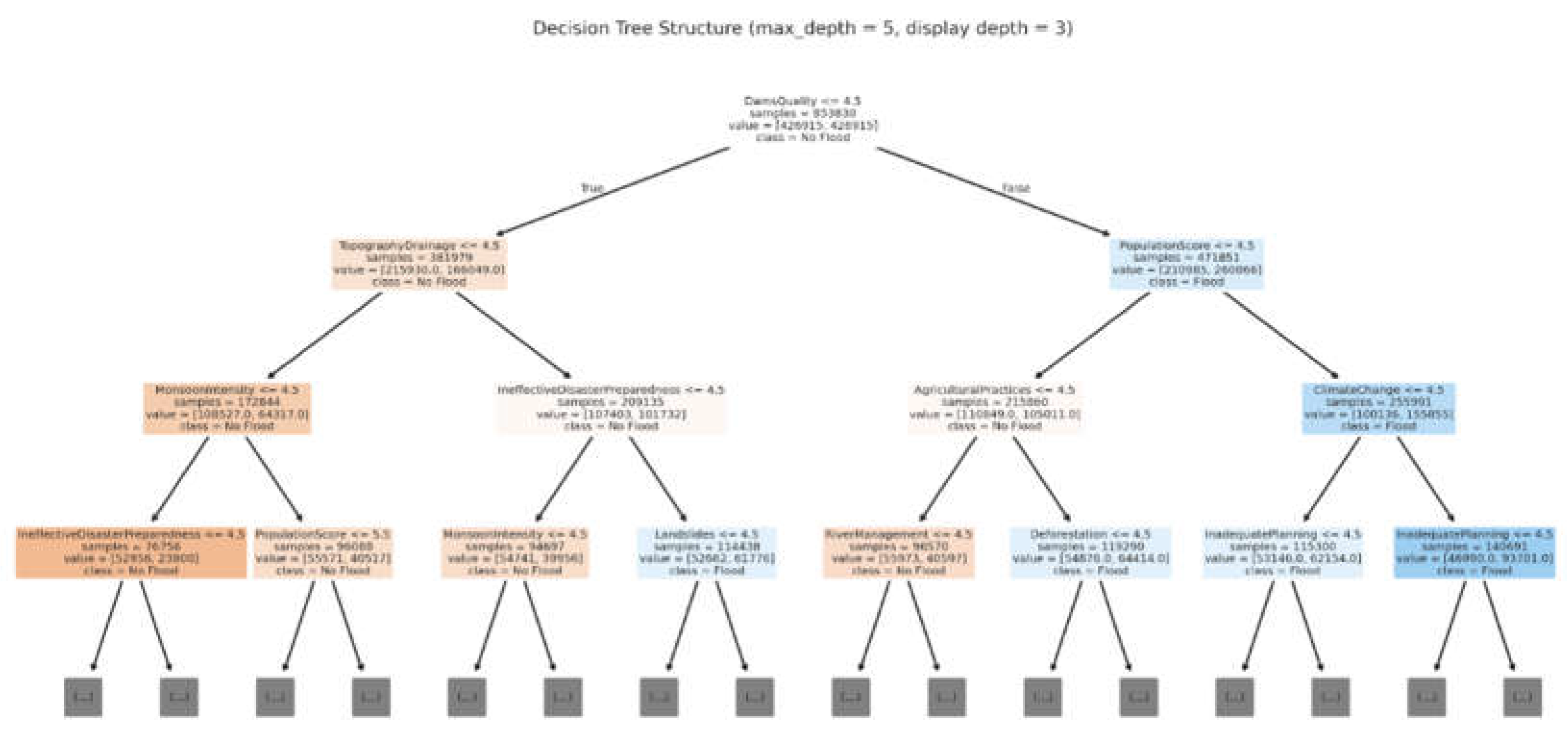
Figure A2.
Confusion matrices for the Decision Tree classifier on the training (left) and independent test (right) partitions. The stark divergence between the training and test matrices quantifies the severe overfitting inherent to the unpruned tree structure. Furthermore, the test matrix highlights an elevated false-negative rate, confirming the model's inability to generalize the complex, additive interactions of the composite risk indices.
Figure A2.
Confusion matrices for the Decision Tree classifier on the training (left) and independent test (right) partitions. The stark divergence between the training and test matrices quantifies the severe overfitting inherent to the unpruned tree structure. Furthermore, the test matrix highlights an elevated false-negative rate, confirming the model's inability to generalize the complex, additive interactions of the composite risk indices.
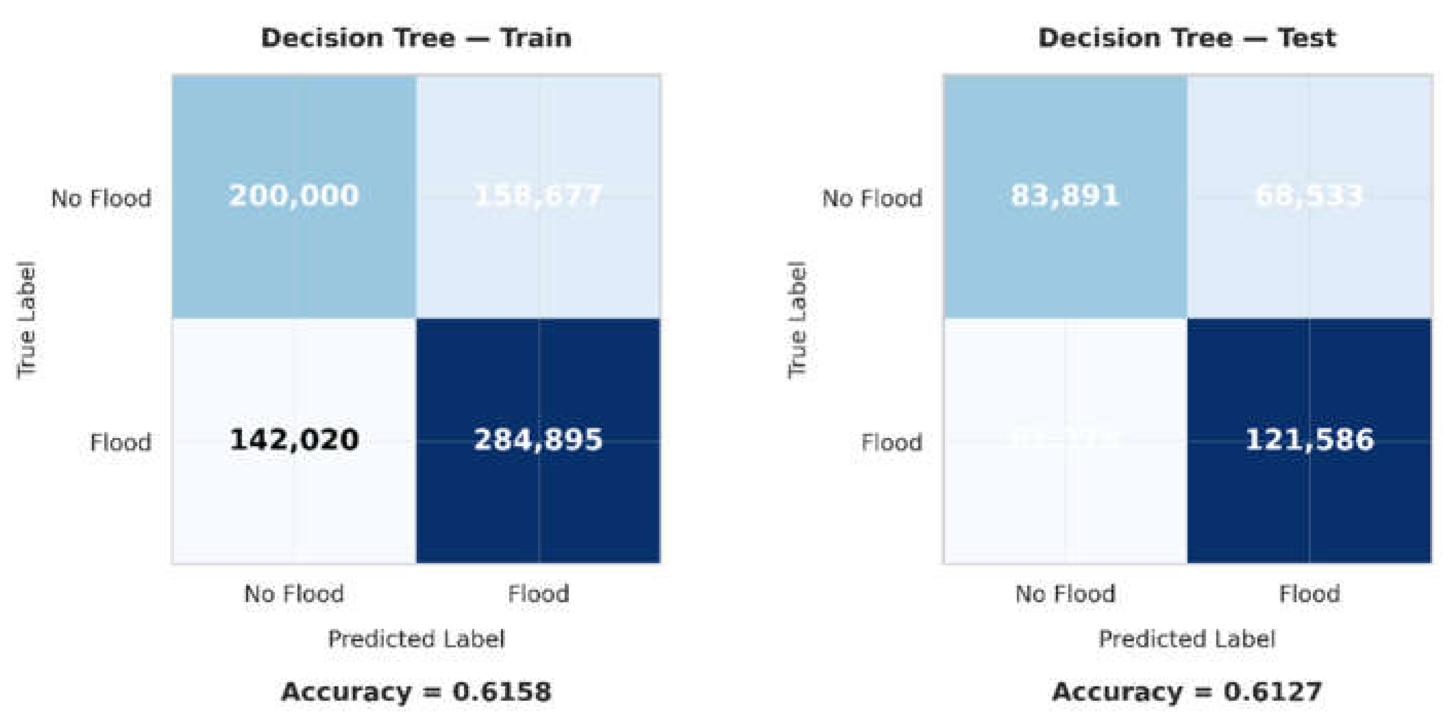
Figure A3.
Feature importance scores from the Random Forest classifier, quantified by the mean decrease in Gini impurity. Despite its lower overall predictive accuracy compared to Logistic Regression, the Random Forest successfully isolates the same dominant hydro-environmental drivers (e.g., Deforestation, DamsQuality). This confirms that the ensemble captures the underlying physical signal, albeit with less optimal decision boundary calibration.
Figure A3.
Feature importance scores from the Random Forest classifier, quantified by the mean decrease in Gini impurity. Despite its lower overall predictive accuracy compared to Logistic Regression, the Random Forest successfully isolates the same dominant hydro-environmental drivers (e.g., Deforestation, DamsQuality). This confirms that the ensemble captures the underlying physical signal, albeit with less optimal decision boundary calibration.
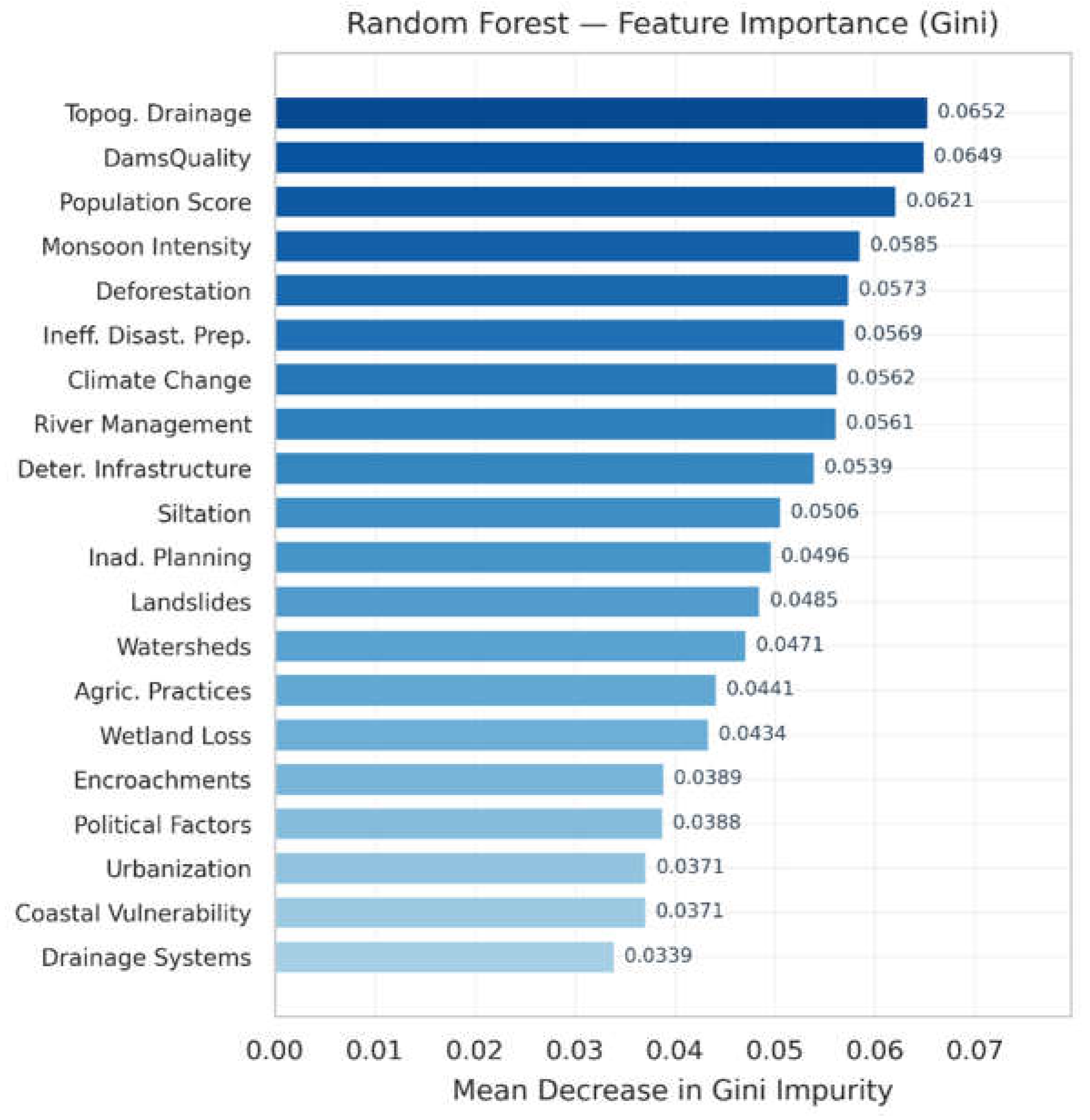
Figure A4.
Confusion matrices for the Random Forest classifier on the training (left) and independent test (right) partitions. The bootstrap aggregation mechanism effectively mitigates the extreme overfitting observed in the standalone Decision Tree. However, the test partition still exhibits a persistent recall deficit compared to the linear baseline, reflecting the variance introduced by deep tree ensembles on discrete feature spaces.
Figure A4.
Confusion matrices for the Random Forest classifier on the training (left) and independent test (right) partitions. The bootstrap aggregation mechanism effectively mitigates the extreme overfitting observed in the standalone Decision Tree. However, the test partition still exhibits a persistent recall deficit compared to the linear baseline, reflecting the variance introduced by deep tree ensembles on discrete feature spaces.
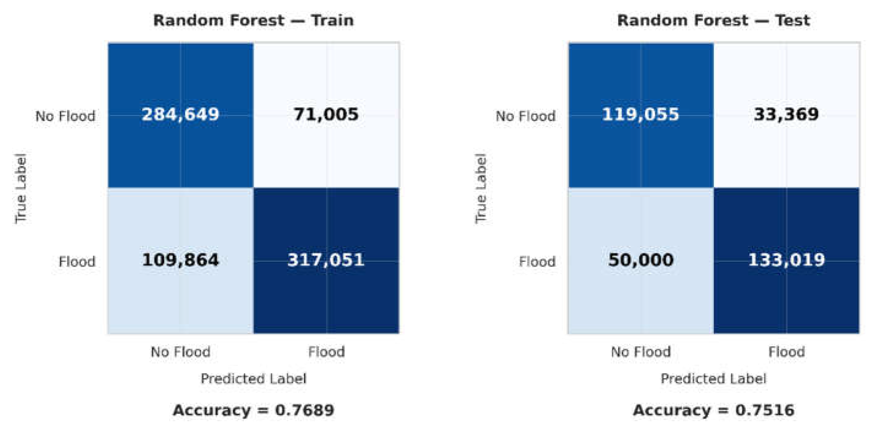
Figure A5.
Confusion matrices for the Gradient Boosting Machine (GBM) on the training (left) and independent test (right) partitions. The sequential functional gradient descent improves the true positive rate on the test set relative to Random Forest. The matrix demonstrates a tighter alignment between training and test distributions, indicating that iterative pseudo-residual fitting partially adapts to the ordinal step-functions, though it still trails the linear model in balanced accuracy.
Figure A5.
Confusion matrices for the Gradient Boosting Machine (GBM) on the training (left) and independent test (right) partitions. The sequential functional gradient descent improves the true positive rate on the test set relative to Random Forest. The matrix demonstrates a tighter alignment between training and test distributions, indicating that iterative pseudo-residual fitting partially adapts to the ordinal step-functions, though it still trails the linear model in balanced accuracy.
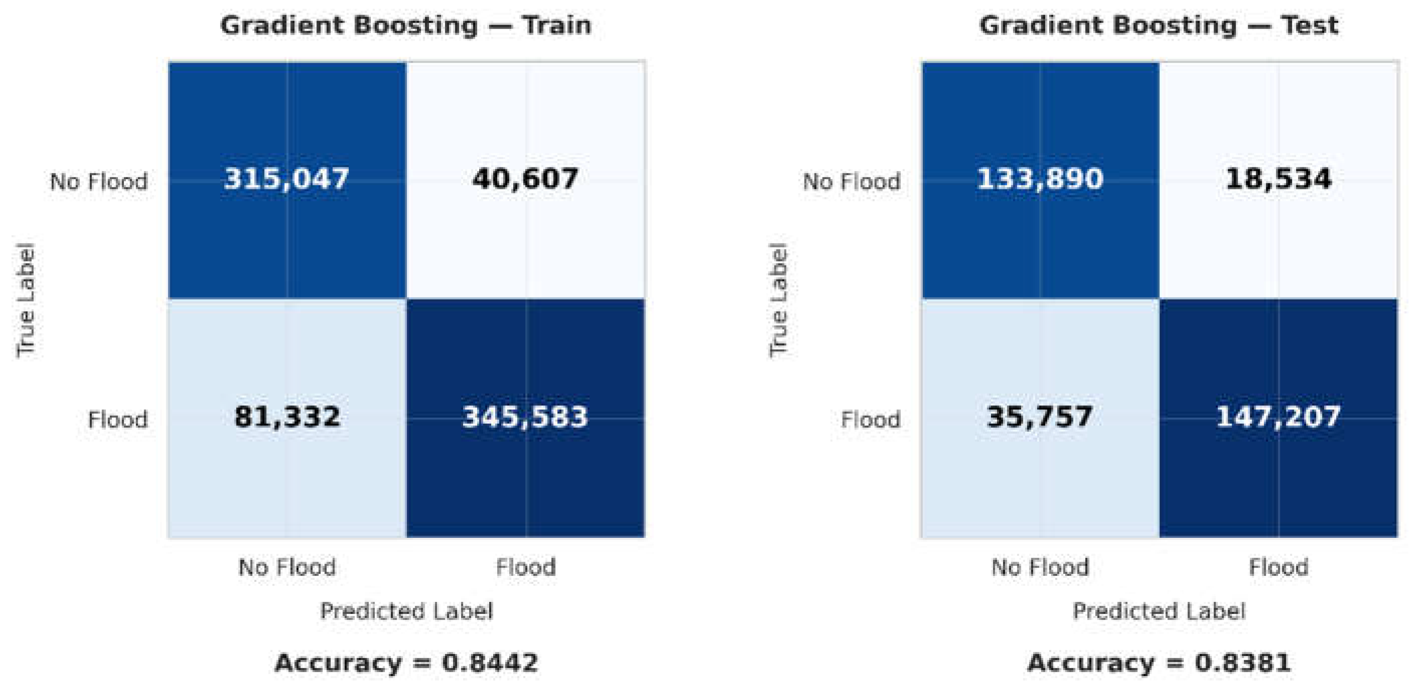
Figure A6.
Feature importance scores from the LightGBM classifier, quantified by total split gain. The histogram-based, leaf-wise growth strategy allocates the highest information gain to the exact same physical predictors identified by the Random Forest and Logistic Regression models. This structural alignment reinforces the physical interpretability of the composite indices, independent of the specific tree-building heuristic.
Figure A6.
Feature importance scores from the LightGBM classifier, quantified by total split gain. The histogram-based, leaf-wise growth strategy allocates the highest information gain to the exact same physical predictors identified by the Random Forest and Logistic Regression models. This structural alignment reinforces the physical interpretability of the composite indices, independent of the specific tree-building heuristic.
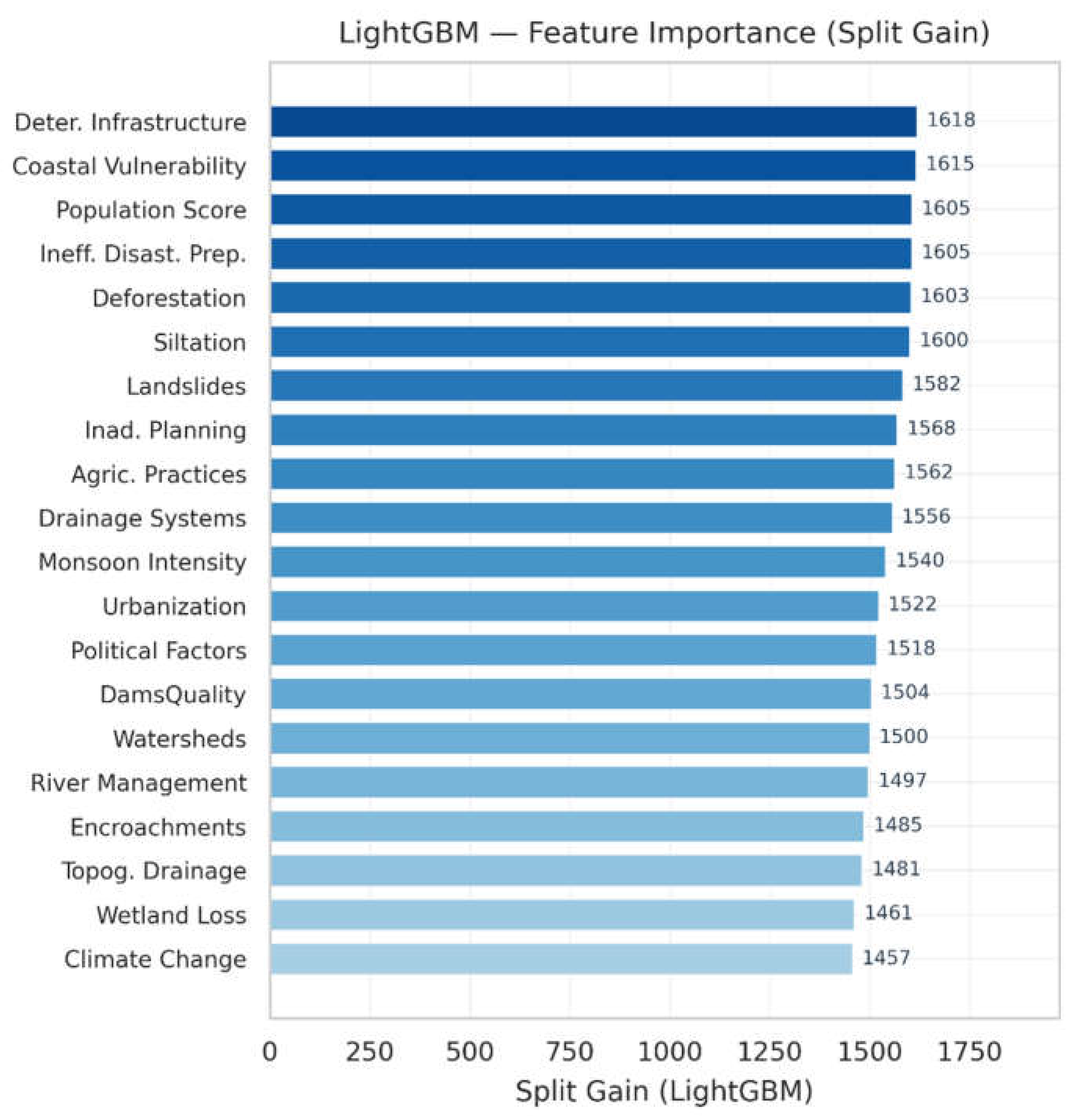
Figure A7.
Confusion matrices for the LightGBM classifier on the training (left) and independent test (right) partitions. While LightGBM achieves a high overall accuracy on the test set, the confusion matrix reveals a slight compression in recall. This reflects the algorithm's global loss optimization, which prioritizes minimizing the aggregate binary cross-entropy over balancing the asymmetric costs of flood early warning.
Figure A7.
Confusion matrices for the LightGBM classifier on the training (left) and independent test (right) partitions. While LightGBM achieves a high overall accuracy on the test set, the confusion matrix reveals a slight compression in recall. This reflects the algorithm's global loss optimization, which prioritizes minimizing the aggregate binary cross-entropy over balancing the asymmetric costs of flood early warning.
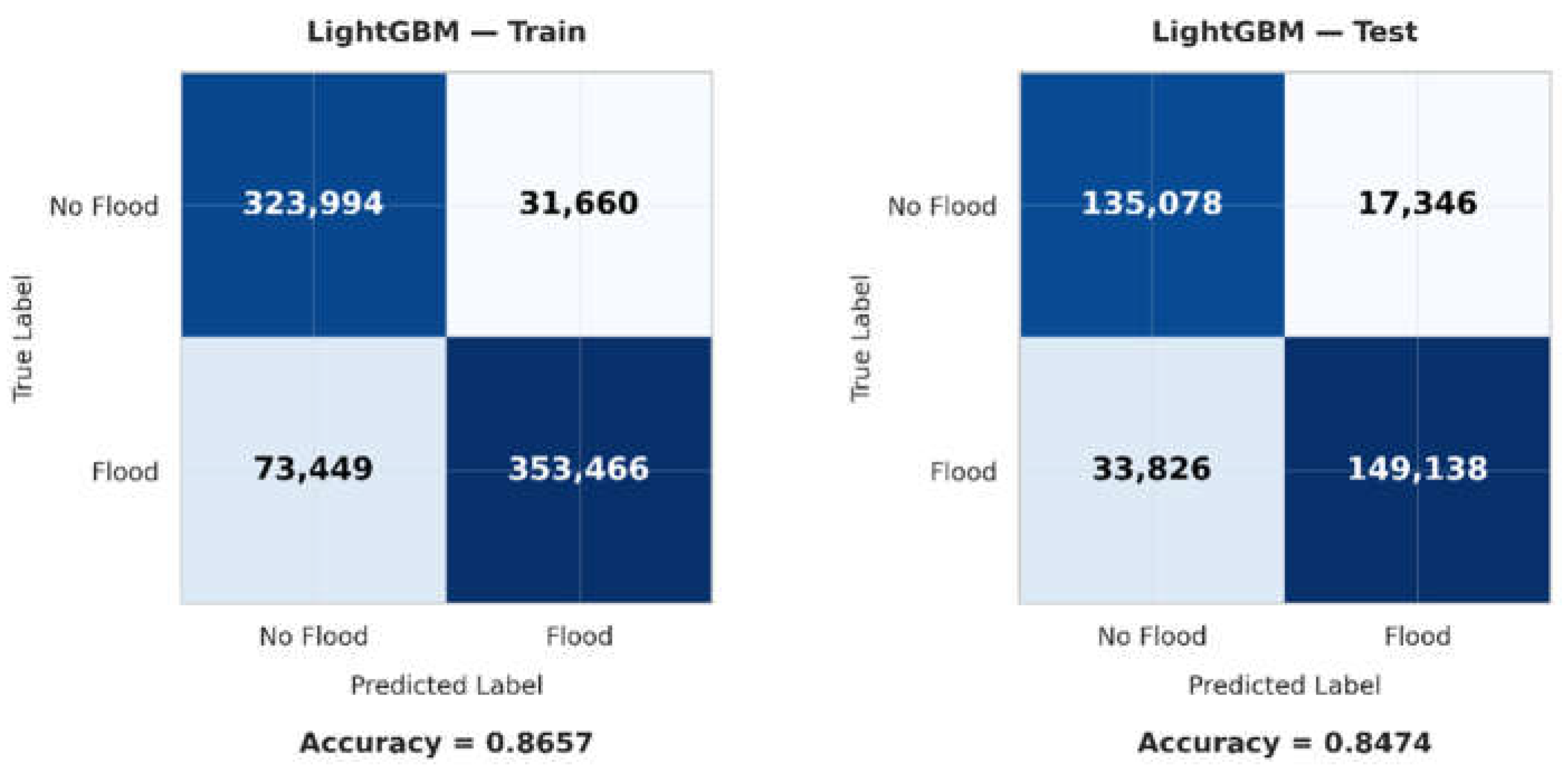
Figure A8.
Confusion matrices for the CatBoost classifier on the training (left) and independent test (right) partitions. Although CatBoost yielded a nominally higher raw accuracy than Logistic Regression in the aggregate metrics, the confusion matrix exposes the operational trade-off: a significantly higher number of false negatives (missed flood events). In flood risk management, where the societal cost of an undetected flood far exceeds that of a false alarm, this matrix reinforces the practical relevance of the linear model within this benchmarking exercise.
Figure A8.
Confusion matrices for the CatBoost classifier on the training (left) and independent test (right) partitions. Although CatBoost yielded a nominally higher raw accuracy than Logistic Regression in the aggregate metrics, the confusion matrix exposes the operational trade-off: a significantly higher number of false negatives (missed flood events). In flood risk management, where the societal cost of an undetected flood far exceeds that of a false alarm, this matrix reinforces the practical relevance of the linear model within this benchmarking exercise.
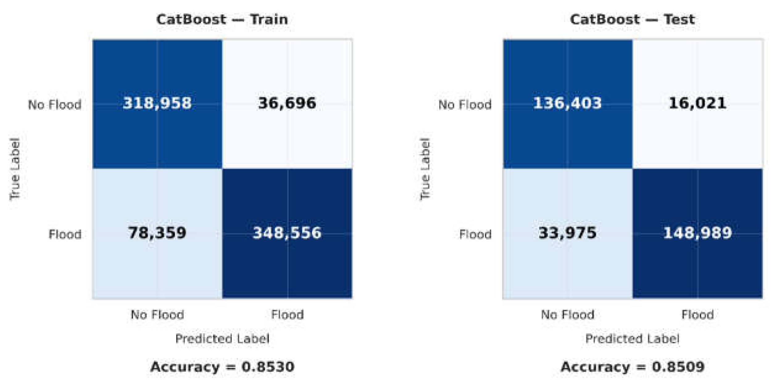
Figure A9.
Cross-model normalized feature importance heatmap comparing split-gain and Gini-decrease metrics across all evaluated tree-based ensembles. This synthesis demonstrates a strong structural consensus among the non-linear architectures. Despite their distinct algorithmic formulations (bagging vs. boosting, level-wise vs. leaf-wise growth), all tree ensembles converge on the same hierarchical ranking of predictive variables, validating that the hydro-environmental signal within the ordinal indices is robust and unambiguously captured by the data-generating process.
Figure A9.
Cross-model normalized feature importance heatmap comparing split-gain and Gini-decrease metrics across all evaluated tree-based ensembles. This synthesis demonstrates a strong structural consensus among the non-linear architectures. Despite their distinct algorithmic formulations (bagging vs. boosting, level-wise vs. leaf-wise growth), all tree ensembles converge on the same hierarchical ranking of predictive variables, validating that the hydro-environmental signal within the ordinal indices is robust and unambiguously captured by the data-generating process.
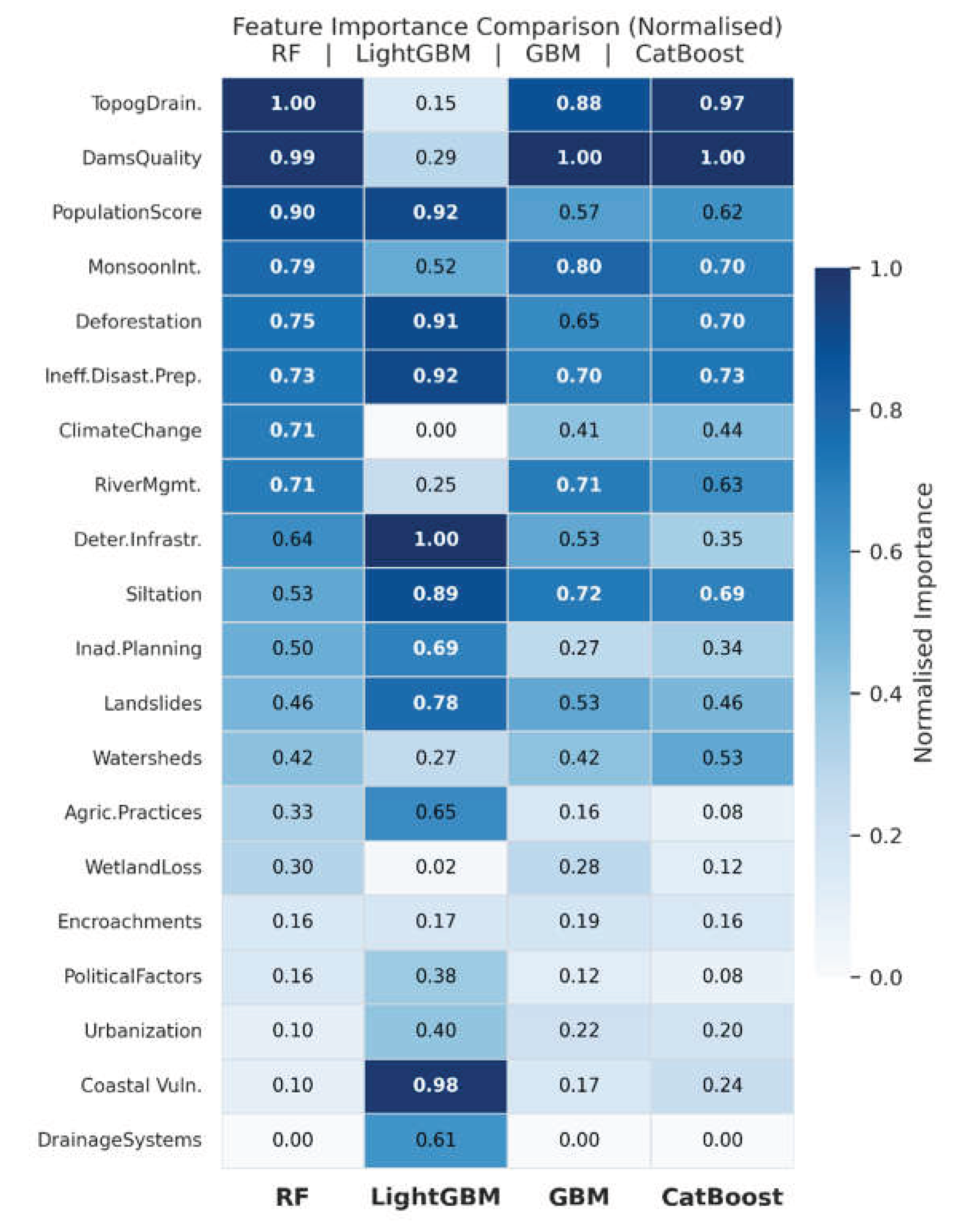
Appendix C. Supplementary Exploratory Data Analysis
To keep the main Results section focused on the model comparison and calibration analysis that this revision foregrounds, four descriptive figures referenced in Section 3.2 are reported here rather than in the main text: Tukey outlier-fence box plots for MonsoonIntensity, PopulationScore, and FloodProbability (Figure A10); the full lower-triangle Pearson correlation heatmap across all 20 predictors and the target (n = 100,000 subsample; Figure A11); the frequency distribution and box plot of FloodProbability (Figure A12, provided here for completeness alongside the three-panel view already given as Figure 2 in the main text); and the ranked absolute mean class difference, |mean(Class 1) – mean(Class 0)|, used as a model-free discriminatory-power index for each predictor (Figure A13).
Figure A10.
Box plots with Tukey outlier bounds (1.5 × IQR fence) for MonsoonIntensity, PopulationScore, and FloodProbability (n > 1 M). Dotted red lines: Q1 − 1.5 × IQR and Q3 + 1.5 × IQR fences. Outlier counts annotated below each panel. The corresponding outlier statics are: (a) MonsoonIntensity: 9244 outliers; bounds: [–1.50, 10.50]. (b) PopulationScore: 9290 outliers; bounds: [–1.50, 10.50]. (c) FloodProbability: 5579 outliers; bounds: [0.36, 0.65].
Figure A10.
Box plots with Tukey outlier bounds (1.5 × IQR fence) for MonsoonIntensity, PopulationScore, and FloodProbability (n > 1 M). Dotted red lines: Q1 − 1.5 × IQR and Q3 + 1.5 × IQR fences. Outlier counts annotated below each panel. The corresponding outlier statics are: (a) MonsoonIntensity: 9244 outliers; bounds: [–1.50, 10.50]. (b) PopulationScore: 9290 outliers; bounds: [–1.50, 10.50]. (c) FloodProbability: 5579 outliers; bounds: [0.36, 0.65].
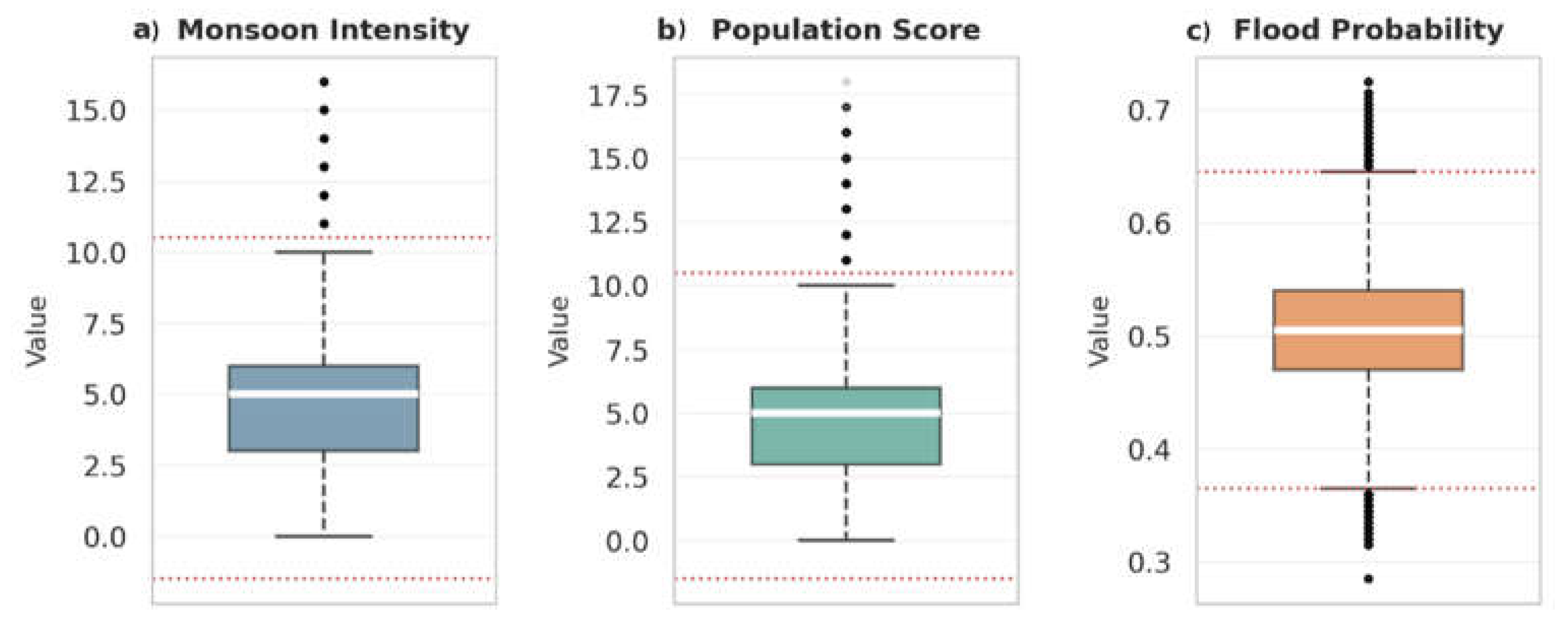
Figure A11.
Lower-triangle Pearson correlation heatmap for all 20 hydro-environmental predictor variables and FloodProbability (n = 100,000 random sample). Near-zero inter-predictor correlations support the low-collinearity reading discussed in Section 3.2.
Figure A11.
Lower-triangle Pearson correlation heatmap for all 20 hydro-environmental predictor variables and FloodProbability (n = 100,000 random sample). Near-zero inter-predictor correlations support the low-collinearity reading discussed in Section 3.2.
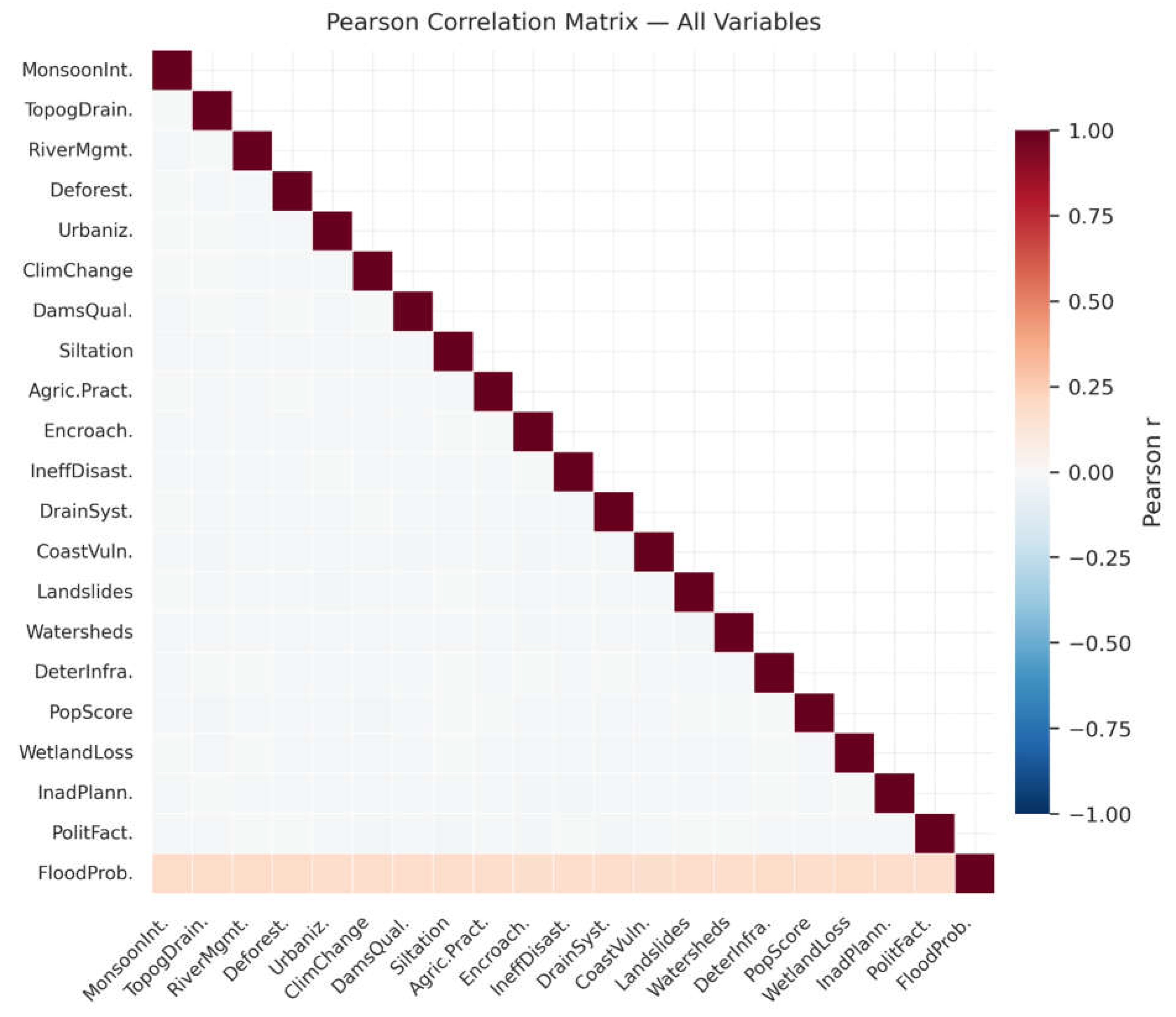
Figure A12.
Frequency distribution and box plot of FloodProbability (n > 1 M). Mean = 0.5045, SD = 0.0510, Median = 0.5050.
Figure A12.
Frequency distribution and box plot of FloodProbability (n > 1 M). Mean = 0.5045, SD = 0.0510, Median = 0.5050.
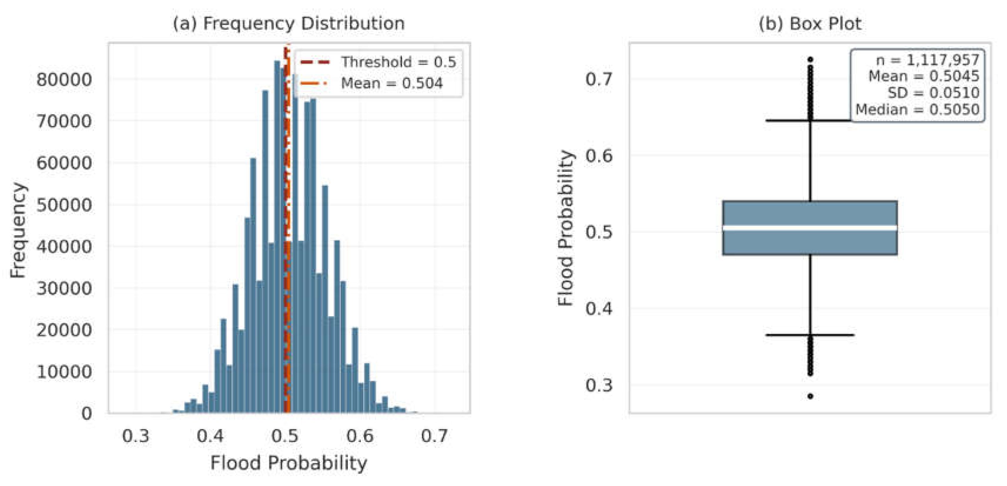
Figure A13.
Absolute mean difference |Mean(Class 1) − Mean(Class 0)| as a model-free discriminatory power index for each predictor, sorted in descending order.
Figure A13.
Absolute mean difference |Mean(Class 1) − Mean(Class 0)| as a model-free discriminatory power index for each predictor, sorted in descending order.
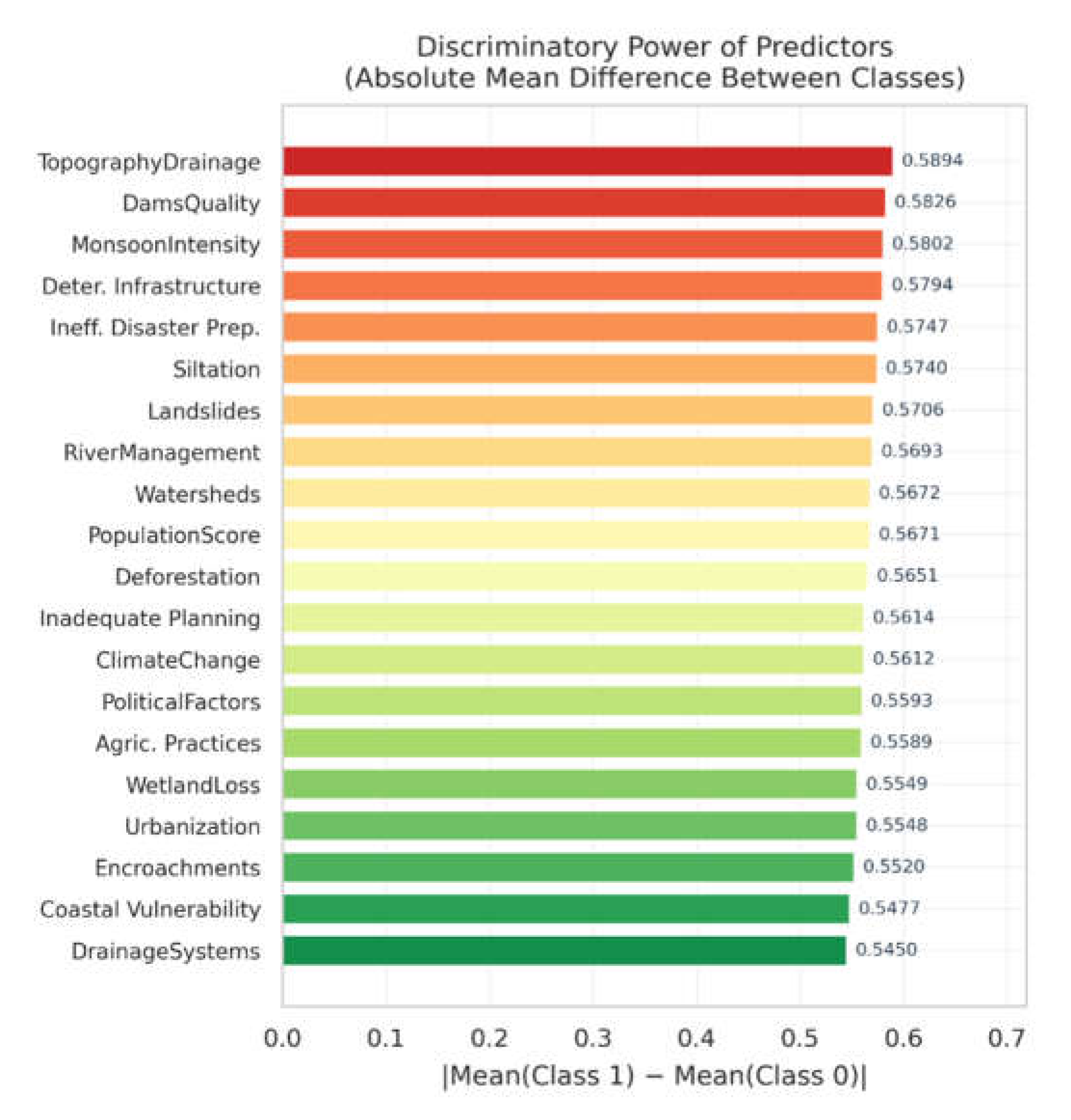
Appendix D. Reproducible Pipeline, Stage II (FEMA NRI, County)
The listing below is not the full Stage II pipeline; it isolates the two elements that carry the scientific weight of this stage — the exposure-confound diagnostic that determined how the target variable had to be built, and the spatial leave-one-region-out cross-validation that produced the collapse reported in Section 3.11. Data cleaning, the six-classifier hyperparameter definitions (identical to Appendix A.6), and calibration code (identical in structure to Appendix A.12) are omitted here for brevity and are unchanged from Stage I in form. RANDOM_STATE = 100 throughout.
# ─ D.1 Exposure-confound diagnostic (decides the target definition) ─────────
r_pop, _ = pointbiserialr(df['IFLD_EALS_high'], df['POPULATION'])
r_hlr, _ = pointbiserialr(df['FloodRiskHigh'], df['POPULATION'])
print(f"Population r with $-loss target : {r_pop:.2f}") # 0.63 -> confounded
print(f"Population r with rate target : {r_hlr:.2f}") # -0.03 -> clean
# ─ D.2 Target: Historic Loss Ratio Rating, not raw dollar loss ──────────────
df['FloodRiskHigh'] = df['IFLD_HLRR'].isin(
['Relatively High', 'Very High']).astype(int)
# ─ D.3 Six-classifier holdout benchmark (hyperparameters per Appendix A.6) ──
for name, mdl in models.items():
mdl.fit(X_bal, y_bal)
results.append(evaluate(name, mdl, X_test, y_test))
# ─ D.4 Spatial leave-one-region-out cross-validation ────────────────────────
for region in ['South', 'West', 'Midwest', 'Northeast']:
train = df[df.REGION != region]; test = df[df.REGION == region]
X_tr, y_tr = train[PREDICTORS].values, train['FloodRiskHigh'].values
X_te, y_te = test[PREDICTORS].values, test['FloodRiskHigh'].values
X_bal_r, y_bal_r = RandomOverSampler(random_state=100).fit_resample(X_tr, y_tr)
for name, mdl in {'Logistic Regression': lr, 'Random Forest': rf,
'LightGBM': lgbm}.items():
mdl.fit(X_bal_r, y_bal_r)
proba = mdl.predict_proba(X_te)[:, 1]
spatial_rows.append({'region': region, 'model': name,
'AUC': roc_auc_score(y_te, proba)})
Appendix E. Reproducible Pipeline, Stage III (FEMA NRI, Census Tract)
Target and predictor construction at tract level are identical in logic to Appendix D.1-D.2 and are not repeated. The listing below isolates what is genuinely new at this stage: merging two independently downloaded extracts into a single verified dataset and confirming that the spatial collapse observed at county level (Appendix D.4) reproduces at a sample size twenty-seven times larger. RANDOM_STATE = 100 throughout.
# ─ E.1 Merge two independently downloaded extracts; verify integrity ────────
df1 = pd.read_csv('NRI_Table_CensusTracts_1de2.csv')
df2 = pd.read_csv('NRI_Table_CensusTracts_2de2.csv')
assert list(df1.columns) == list(df2.columns)
df = pd.concat([df1, df2], ignore_index=True)
assert df['TRACTFIPS'].duplicated().sum() == 0 # 0 duplicates -> OK
assert df.shape == (85154, 467) # full extract confirmed
# ─ E.2 Same cleaning and target logic as Appendix D.1-D.2, at tract scale ───
# (territories excluded, "No Rating" dropped, FloodRiskHigh from IFLD_HLRR)
# working sample: n = 84,034 tracts, prevalence = 25.7%
# ─ E.3 Holdout benchmark, six classifiers, n = 25,211 test tracts ───────────
for name, mdl in models.items():
mdl.fit(X_bal, y_bal)
results.append(evaluate(name, mdl, X_test, y_test))
# Random Forest AUC = 0.8507 (county: 0.7855); LR AUC = 0.7449 (county: 0.6680)
# ─ E.4 Spatial leave-one-region-out cross-validation, tract level ──────────
for region in ['South', 'West', 'Midwest', 'Northeast']:
train = df[df.REGION != region]; test = df[df.REGION == region]
# training folds: 51,895-69,353 tracts, an order of magnitude above
# any county-level fold in Appendix D.4
X_bal_r, y_bal_r = RandomOverSampler(random_state=100).fit_resample(
train[PREDICTORS].values, train['FloodRiskHigh'].values)
for name, mdl in {'Logistic Regression': lr, 'Random Forest': rf,
'LightGBM': lgbm}.items():
mdl.fit(X_bal_r, y_bal_r)
proba = mdl.predict_proba(test[PREDICTORS].values)[:, 1]
spatial_rows.append({'region': region, 'model': name,
'AUC': roc_auc_score(test['FloodRiskHigh'].values, proba)})
# mean spatial AUC: LR = 0.638, RF = 0.590 -> collapse reproduces (Table 15)
References
- CRED; UNDRR. Human Cost of Disasters: An Overview of the Last 20 Years 2000–2019; Centre for Research on the Epidemiology of Disasters: Brussels, 2020. [Google Scholar]
- IPCC. Climate Change 2021: The Physical Science Basis. Contribution of Working Group I to the Sixth Assessment Report; Cambridge University Press: Cambridge, UK and New York, NY, USA, 2021. [Google Scholar] [CrossRef]
- Teng, J.; Jakeman, A.J.; Vaze, J.; Croke, B.F.W.; Dutta, D.; Kim, S. Flood inundation modelling: A review of methods, recent advances and uncertainty analysis. Environ. Model. Softw. 2017, 90, 201–216. [Google Scholar] [CrossRef]
- Mosavi, A.; Ozturk, P.; Chau, K.-W. Flood prediction using machine learning models: Literature review. Water 2018, 10, 1536. [Google Scholar] [CrossRef]
- Benavides-Muñoz, H. M.; Román-Aguilar, K. M. Hydrodynamic modeling and flood mitigation strategies in an Andean Valley City. PLoS Water 2025, 4, 7. [Google Scholar] [CrossRef]
- Boulmaiz, T.; Guermoui, M.; Boutaghane, H. Impact of training data size on the LSTM performances for rainfall–runoff modeling. Model. Earth Syst. Environ. 2020, 6, 2153–2164. [Google Scholar] [CrossRef]
- Tyralis, H.; Papacharalampous, G.; Langousis, A. A brief review of random forests for water scientists and practitioners and their recent history in water resources. Water 2019, 11, 910. [Google Scholar] [CrossRef]
- Li, Z.; Liu, H.; Luo, C.; Fu, G. Assessing surface water flood risks in urban areas using machine learning. Water 2021, 13, 3520. [Google Scholar] [CrossRef]
- Bui, D.T.; Hoang, N.-D.; Martínez-Álvarez, F.; Ngo, P.-T.T.; Hoa, P.V.; Pham, T.D.; Samui, P.; Costache, R. A novel deep learning neural network approach for predicting flash flood susceptibility: A case study at a high frequency tropical storm area. Sci. Total Environ. 2020, 701, 134413. [Google Scholar] [CrossRef] [PubMed]
- Yin, J.; Yu, D.; Yin, Z.; Liu, M.; He, Q. Evaluating the impact and risk of pluvial flash flood on intra-urban road network: A case study in the city center of Shanghai, China. J. Hydrol. 2016, 537, 138–145. [Google Scholar] [CrossRef]
- Yaseen, Z.M.; El-Shafie, A.; Jaafar, O.; Afan, H.A.; Sayl, K.N. Artificial intelligence based models for stream-flow forecasting: 2000–2015. J. Hydrol. 2015, 530, 829–844. [Google Scholar] [CrossRef]
- Naiyakhalid. Flood Prediction Dataset. Kaggle, 2023. Available online: https://www.kaggle.com/datasets/naiyakhalid/flood-prediction-dataset (accessed on 1 June 2026).
- Walski, T.M.; Chase, D.V.; Savic, D.A.; Grayman, W.; Beckwith, S.; Koelle, E. Advanced Water Distribution Modeling and Management; Haestad Press: Waterbury, CT, USA, 2003. [Google Scholar]
- Benjamini, Y.; Hochberg, Y. Controlling the false discovery rate: A practical and powerful approach to multiple testing. J. R. Stat. Soc. Ser. B 1995, 57, 289–300. [Google Scholar] [CrossRef]
- Hosmer, D.W.; Lemeshow, S.; Sturdivant, R.X. Applied Logistic Regression, 3rd ed.; Wiley: New York, NY, USA, 2013. [Google Scholar] [CrossRef]
- Chen, T.; Guestrin, C. XGBoost: A scalable tree boosting system. In Proceedings of the 22nd ACM SIGKDD International Conference on Knowledge Discovery and Data Mining, San Francisco, CA, USA, 13–17 August 2016; pp. 785–794. [Google Scholar] [CrossRef]
- Chicco, D.; Jurman, G. The advantages of the Matthews correlation coefficient (MCC) over F1 score and accuracy in binary classification evaluation. BMC Genom. 2020, 21, 6. [Google Scholar] [CrossRef] [PubMed]
- Hanley, J.A.; McNeil, B.J. The meaning and use of the area under a receiver operating characteristic (ROC) curve. Radiology 1982, 143, 29–36. [Google Scholar] [CrossRef] [PubMed]
- Zuzak, C.; Goodenough, E.; Stanton, C.; Mowrer, M.; Sheehan, A.; Roberts, B.; McGuire, P.; Rozelle, J. National Risk Index Technical Documentation; Federal Emergency Management Agency: Washington, DC, USA, 2023; Available online: https://www.fema.gov/about/openfema/data-sets/national-risk-index-data (accessed on 15 December 2025).
- Zuzak, C.; Mowrer, M.; Goodenough, E.; Sheehan, A.; Roberts, B.; McGuire, P.; Rozelle, J. The national risk index: establishing a nationwide baseline for natural hazard risk in the US. Nat. Hazards 2022, 114, 2331–2355. [Google Scholar] [CrossRef]
- Roberts, D.R.; Bahn, V.; Ciuti, S.; Hardy, M.A.; Hauenstein, S.; Guillera-Arroita, G.; Dormann, C.F.; et al. Cross-validation strategies for data with temporal, spatial, hierarchical, or phylogenetic structure. Ecography 2017, 40, 913–929. [Google Scholar] [CrossRef]
- ASCE. Design and Construction of Urban Stormwater Management Systems. In ASCE Manuals of Engineering Practice No. 77; American Society of Civil Engineers: New York, NY, USA, 1992. [Google Scholar]
- Nirupama, N.; Simonovic, S.P. Increase of flood risk due to urbanisation: A Canadian example. Nat. Hazards 2007, 40, 25–41. [Google Scholar] [CrossRef]
- Doocy, S.; Daniels, A.; Murray, S.; Kirsch, T.D. The human impact of floods: A historical review of events 1980–2009 and systematic literature review. In PLoS Curr.; 2013; 5. Available online: https://pmc.ncbi.nlm.nih.gov/articles/PMC3644291/.
- USDA-NRCS. National Engineering Handbook, Part 630: Hydrology; USDA Natural Resources Conservation Service: Washington, DC, USA, 2004. [Google Scholar]
- Ogden, F.L.; Crouch, T.D.; Stallard, R.F.; Hall, J.S. Effect of land cover and use on dry season river runoff, runoff efficiency, and peak storm runoff in the seasonal tropics of central Panama. Water Resour. Res. 2013, 49, 8443–8462. [Google Scholar] [CrossRef]
- Benavides-Muñoz, H.M.; Correa-Escudero, V.; Pucha-Cofrep, D.; Pucha-Cofrep, F. Analysis of Land Use Change and Hydrogeological Parameters in the Andean Semiarid Region of Ecuador. Water 2024, 16, 892. [Google Scholar] [CrossRef]
- USBR. Design of Small Dams, 3rd ed.; U.S. Bureau of Reclamation: Denver, CO, USA, 1987. [Google Scholar]
- Hastie, T.; Tibshirani, R.; Friedman, J. The Elements of Statistical Learning, capítulo 7, "Model Assessment and Selection". In Springer, 2nd ed.; 2009; pp. 219–259. [Google Scholar]
- Ajin, R.S.; Costache, R.; Bărbulescu, A.; Fanti, R.; Segoni, S. Flood Susceptibility Assessment Using Multi-Tier Feature Selection and Ensemble Boosting Machine Learning Models. Water 2025, 17, 2041. [Google Scholar] [CrossRef]
- Lundberg, S.M.; Lee, S.-I. A unified approach to interpreting model predictions. In Advances in Neural Information Processing Systems 30; Guyon, I., Ed.; Curran Associates, Inc.: New York, NY, USA, 2017; pp. 4765–4774. [Google Scholar]
- Lundberg, S.M.; Erion, G.; Chen, H.; DeGrave, A.; Prutkin, J.M.; Nair, B.; Katz, R.; Himmelfarb, J.; Bansal, N.; Lee, S.-I. From local explanations to global understanding with explainable AI for trees. Nat. Mach. Intell. 2020, 2, 56–67. [Google Scholar] [CrossRef] [PubMed]
- United Nations Office for Disaster Risk Reduction (UNDRR). Sendai Framework for Disaster Risk Reduction 2015–2030; UNDRR: Geneva, Switzerland, 2015. [Google Scholar]
- Kratzert, F.; Klotz, D.; Brenner, C.; Schulz, K.; Herrnegger, M. Rainfall–runoff modelling using Long Short-Term Memory (LSTM) networks. Hydrol. Earth Syst. Sci. 2018, 22, 6005–6022. [Google Scholar] [CrossRef]
Figure 1.
Flowchart of the seven-phase machine learning pipeline for probabilistic flood occurrence prediction. Stadium shapes denote terminal nodes; rectangles represent processing steps; diamonds indicate binary decision gates; parallelograms denote data I/O operations; dashed rectangles serve as phase containers. The feedback arc from Phase 5 (AUC ≥ 0.90 decision) to Phase 4 formalizes the iterative model selection protocol.
Figure 1.
Flowchart of the seven-phase machine learning pipeline for probabilistic flood occurrence prediction. Stadium shapes denote terminal nodes; rectangles represent processing steps; diamonds indicate binary decision gates; parallelograms denote data I/O operations; dashed rectangles serve as phase containers. The feedback arc from Phase 5 (AUC ≥ 0.90 decision) to Phase 4 formalizes the iterative model selection protocol.
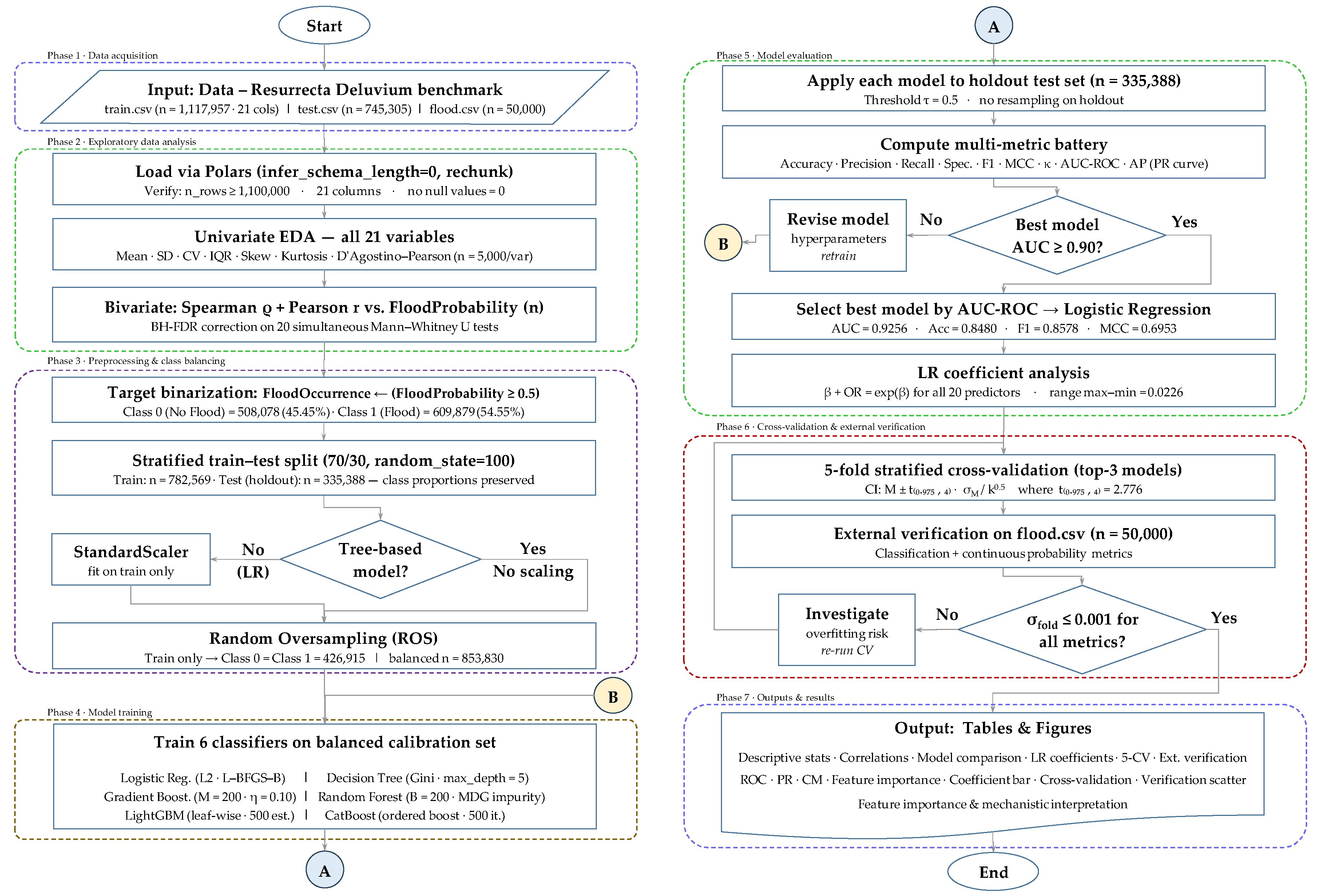
Figure 2.
FloodProbability distribution (n > 1 M): (a) histogram with KDE overlay, mean = 0.504 (dashed line); (b) empirical CDF with classification threshold at 0.5; (c) Normal Q–Q plot. .
Figure 2.
FloodProbability distribution (n > 1 M): (a) histogram with KDE overlay, mean = 0.504 (dashed line); (b) empirical CDF with classification threshold at 0.5; (c) Normal Q–Q plot. .
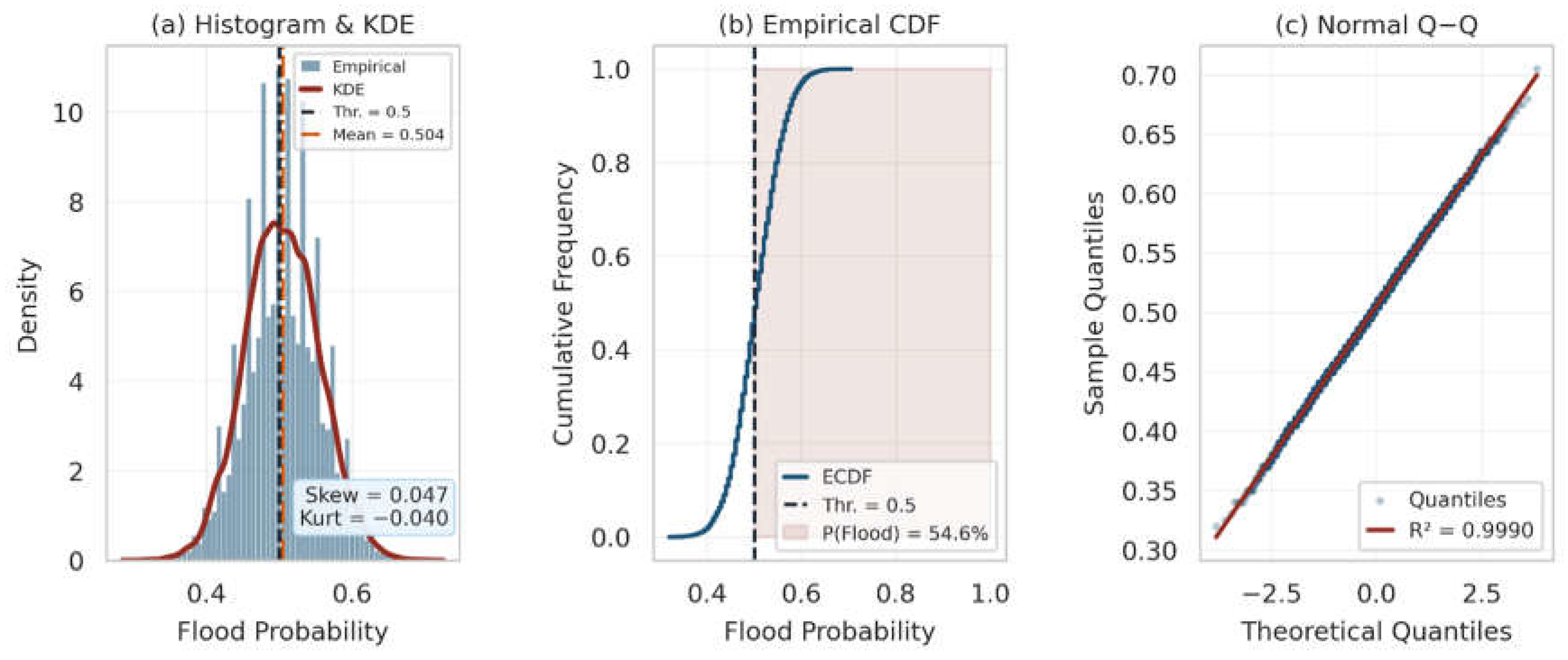
Figure 3.
Class distribution of the binarized target FloodOccurrence (threshold FloodProbability ≥ 0.5): (a) bar chart of absolute counts; (b) proportional pie chart.
Figure 3.
Class distribution of the binarized target FloodOccurrence (threshold FloodProbability ≥ 0.5): (a) bar chart of absolute counts; (b) proportional pie chart.
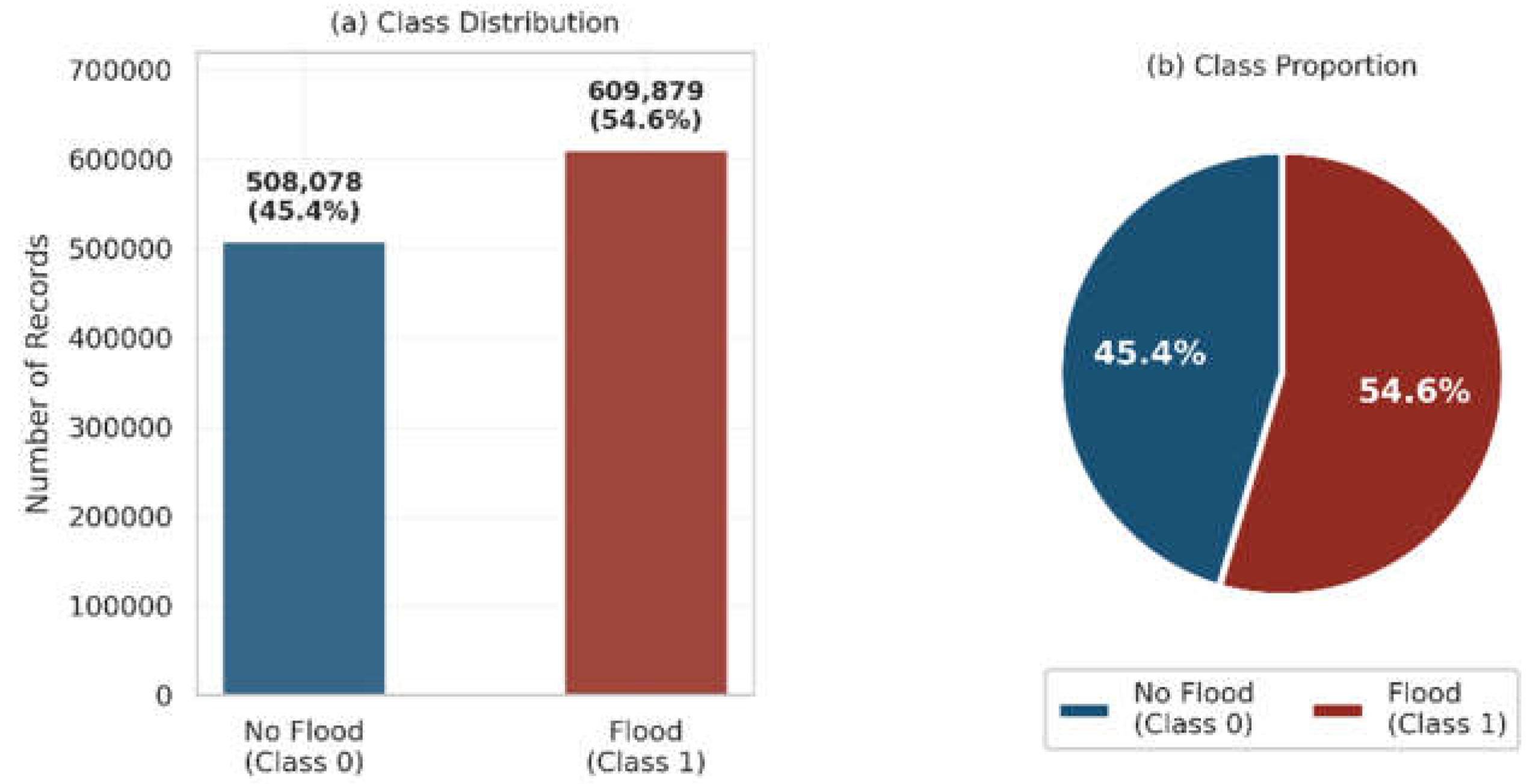
Figure 4.
Pairwise scatter matrix of the six most discriminatory hydro-environmental predictors (n = 3,000 stratified sample). Points are color-coded by flood-risk class, derived from the continuous FloodProbability target: blue denotes low risk (< 0.40), orange indicates medium risk (0.40–0.60), and red represents high risk (> 0.60). Diagonal panels show the univariate frequency distribution for each variable.
Figure 4.
Pairwise scatter matrix of the six most discriminatory hydro-environmental predictors (n = 3,000 stratified sample). Points are color-coded by flood-risk class, derived from the continuous FloodProbability target: blue denotes low risk (< 0.40), orange indicates medium risk (0.40–0.60), and red represents high risk (> 0.60). Diagonal panels show the univariate frequency distribution for each variable.
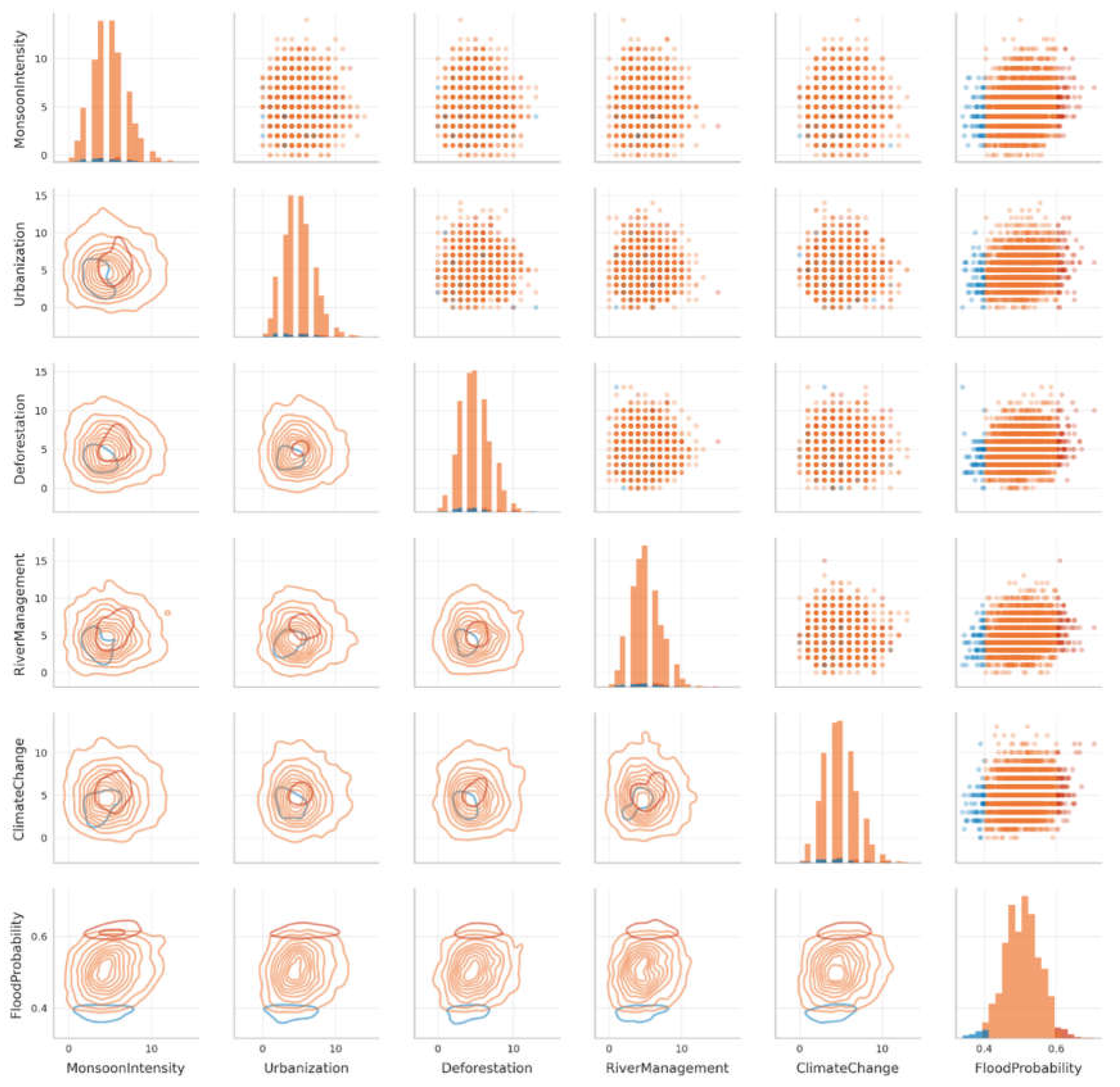
Figure 5.
Hexbin density map of MonsoonIntensity versus DrainageSystems (n = 50,000), colored by mean FloodProbability. Top marginal panel: MonsoonIntensity distribution.
Figure 5.
Hexbin density map of MonsoonIntensity versus DrainageSystems (n = 50,000), colored by mean FloodProbability. Top marginal panel: MonsoonIntensity distribution.
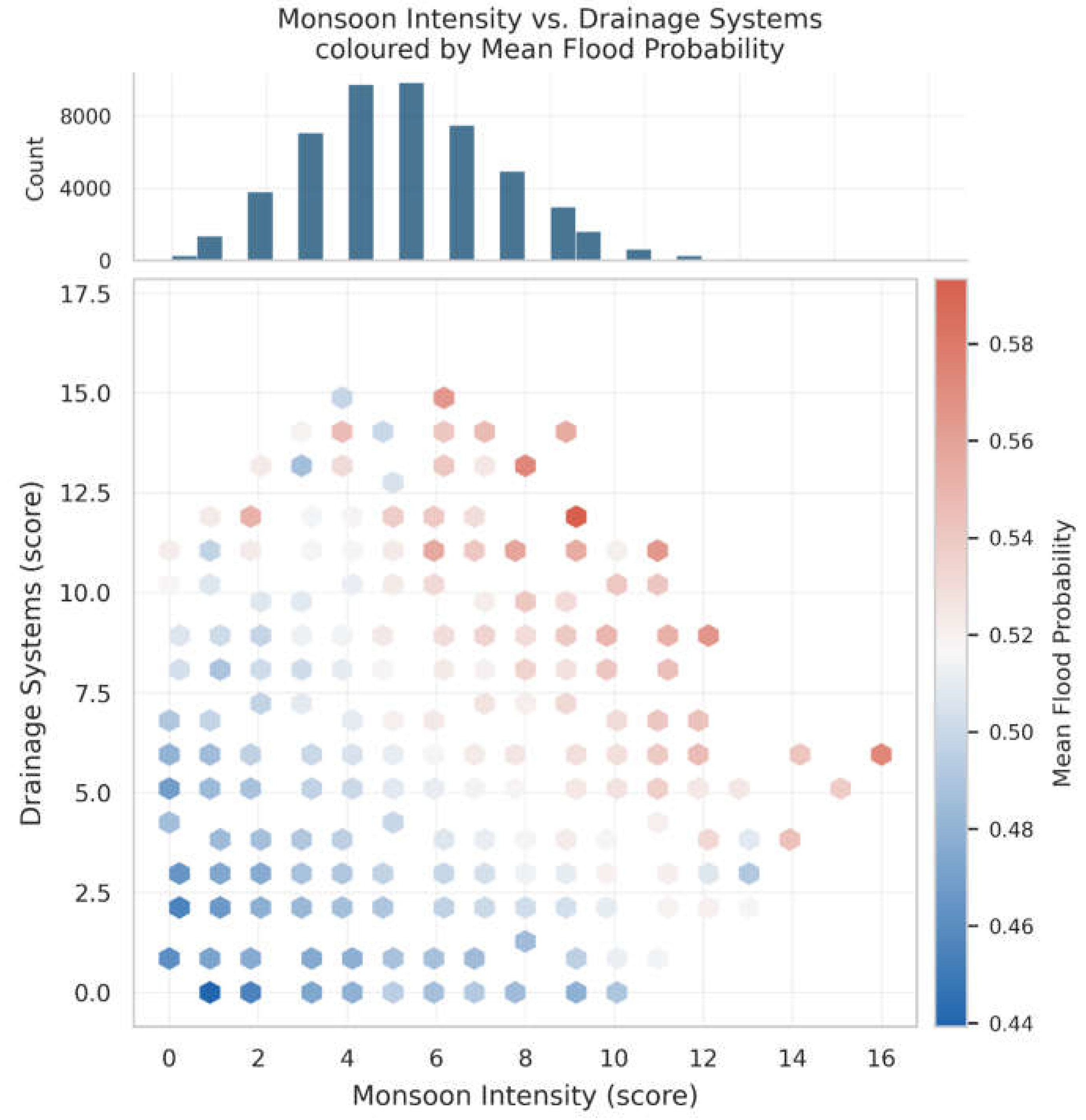
Figure 6.
Violin plots of Urbanization Score stratified by FloodProbability class. Diamond markers: class mean ± SD. Kruskal–Wallis test: p < 0.001.
Figure 6.
Violin plots of Urbanization Score stratified by FloodProbability class. Diamond markers: class mean ± SD. Kruskal–Wallis test: p < 0.001.
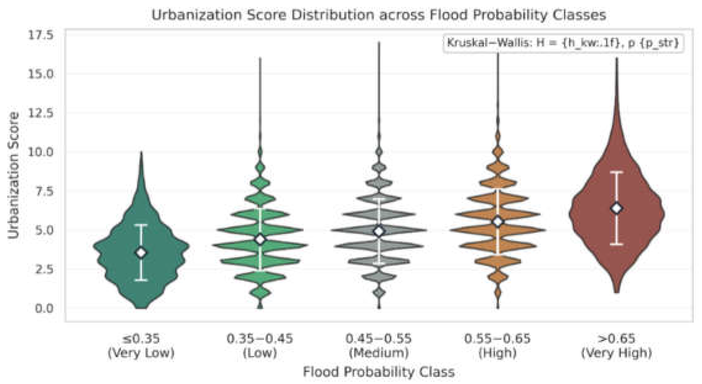
Figure 7.
Spearman rank correlation (ρ) of all 20 hydro-environmental predictors with FloodProbability. All bars positive; *** BH-FDR q < 0.001 for every predictor.
Figure 7.
Spearman rank correlation (ρ) of all 20 hydro-environmental predictors with FloodProbability. All bars positive; *** BH-FDR q < 0.001 for every predictor.
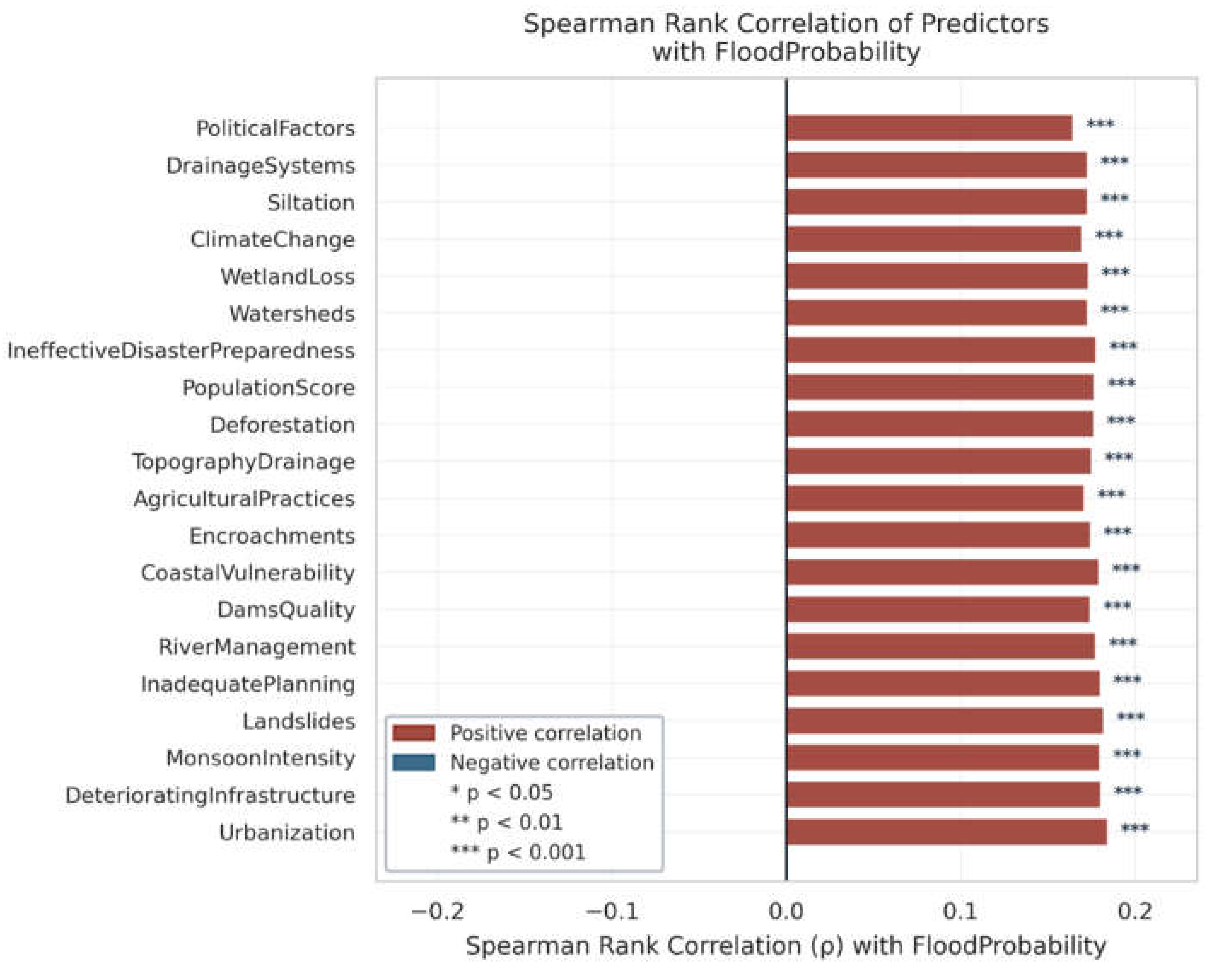
Figure 8.
Box plots of all 20 predictor variables stratified by FloodOccurrence class. Mann–Whitney U test: *** BH-FDR q < 0.001 for all variables.
Figure 8.
Box plots of all 20 predictor variables stratified by FloodOccurrence class. Mann–Whitney U test: *** BH-FDR q < 0.001 for all variables.
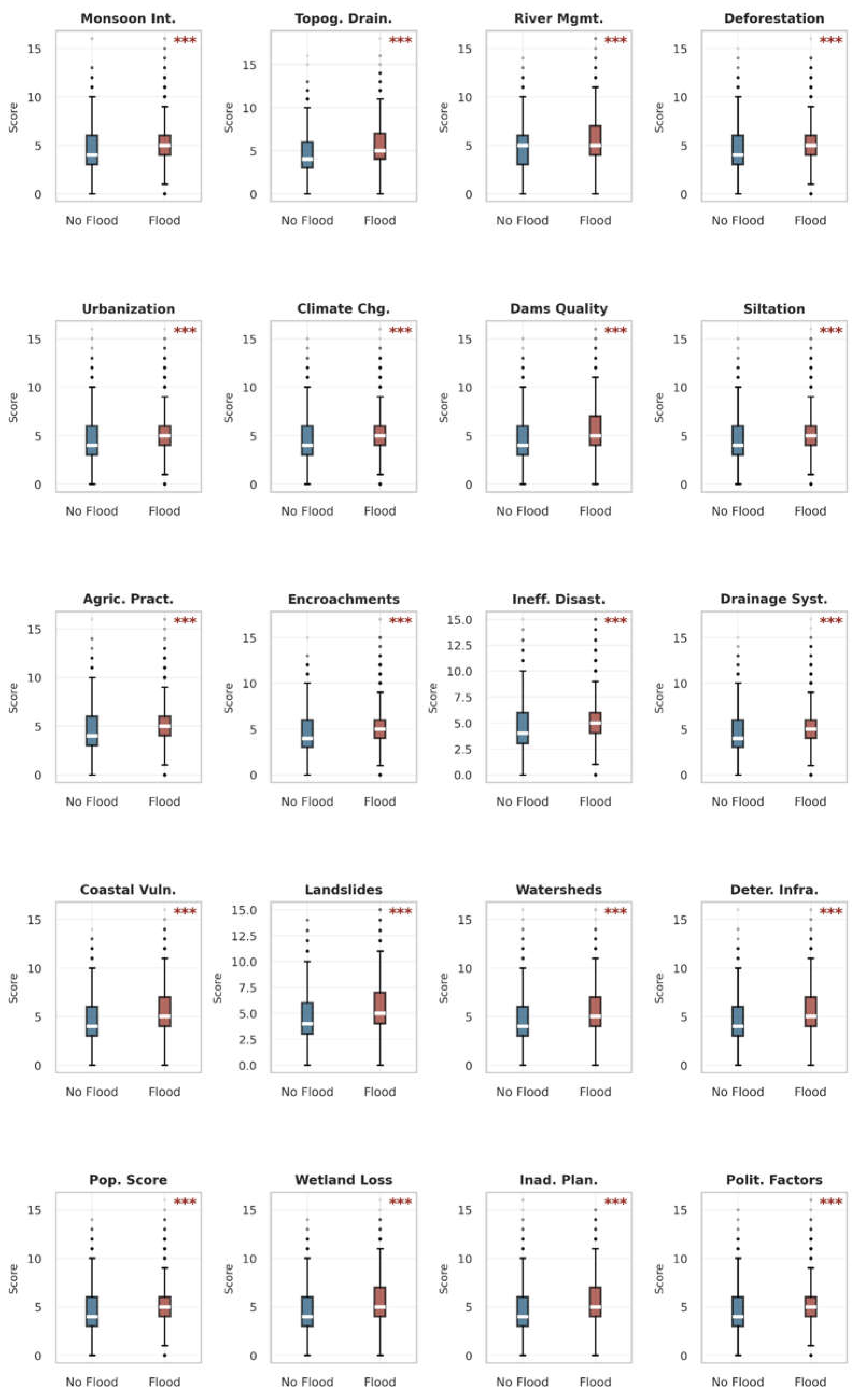
Figure 9.
Radar chart of normalized mean feature scores by FloodOccurrence class (all 20 predictors). The consistently expanded Class 1 (Flood) profile illustrates the uniform discriminatory structure.
Figure 9.
Radar chart of normalized mean feature scores by FloodOccurrence class (all 20 predictors). The consistently expanded Class 1 (Flood) profile illustrates the uniform discriminatory structure.
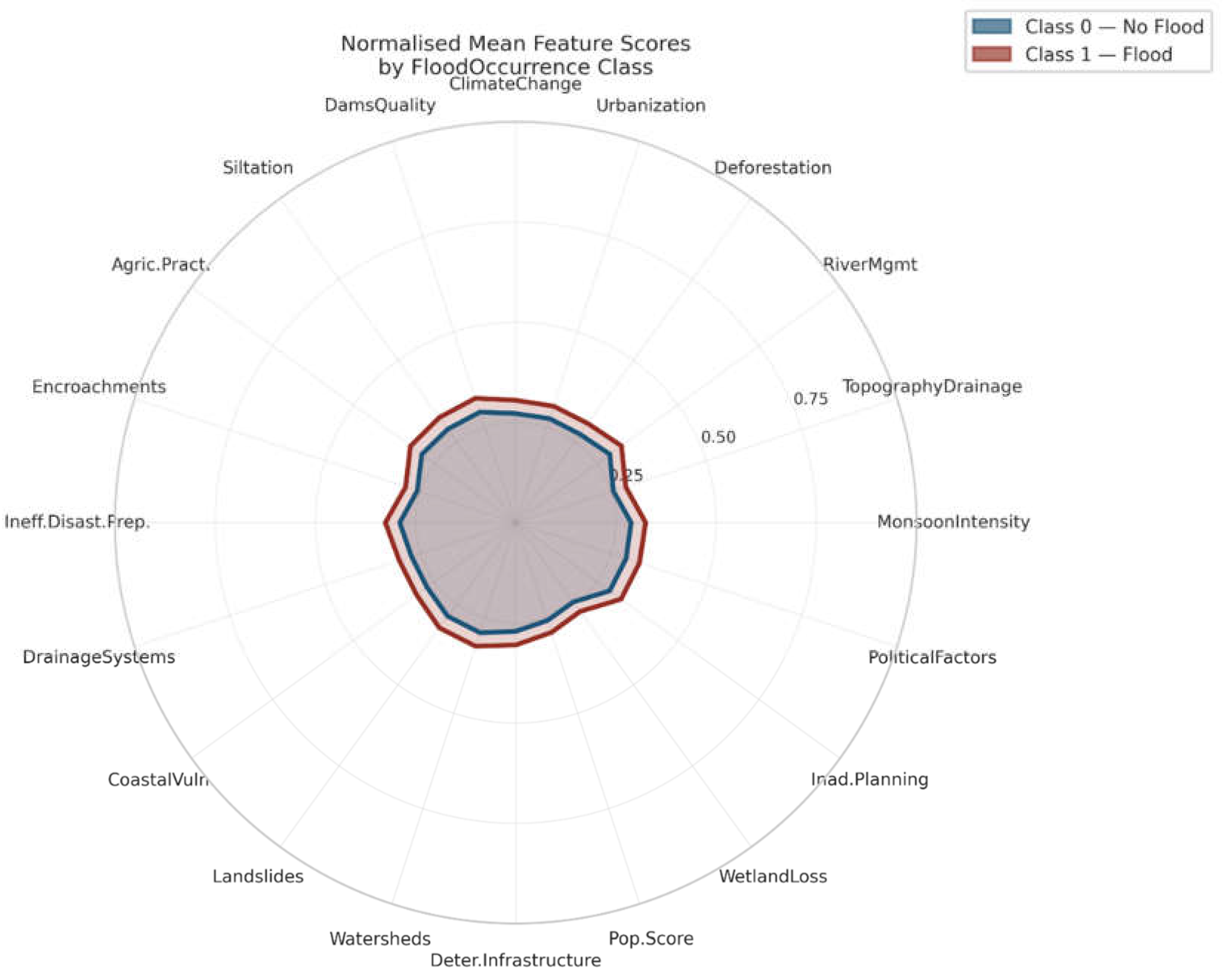
Figure 10.
Class distribution of the training partition (a) before and (b) after Random Oversampling; the external holdout partition and the flood.csv subset were left unmodified throughout.
Figure 10.
Class distribution of the training partition (a) before and (b) after Random Oversampling; the external holdout partition and the flood.csv subset were left unmodified throughout.
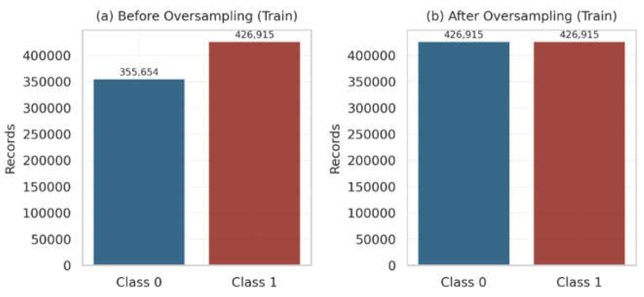
Figure 11.
Comparative ROC curves for all six classifiers on the 30% holdout test partition. Dashed diagonal: random classifier baseline (AUC = 0.500).
Figure 11.
Comparative ROC curves for all six classifiers on the 30% holdout test partition. Dashed diagonal: random classifier baseline (AUC = 0.500).
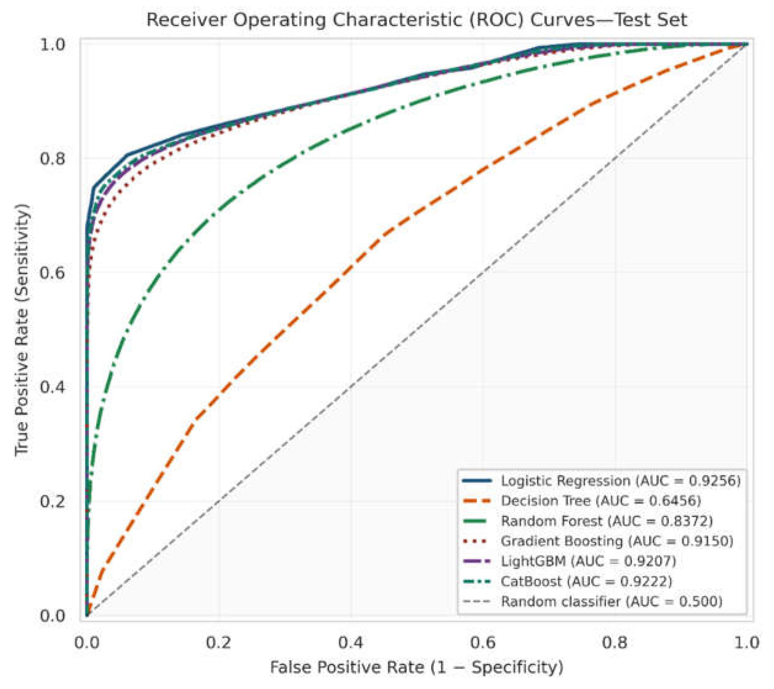
Figure 12.
Multi-metric performance comparison (Accuracy, Precision, Recall, Specificity, F1-score, AUC-ROC) of all six classifiers on the holdout partition.
Figure 12.
Multi-metric performance comparison (Accuracy, Precision, Recall, Specificity, F1-score, AUC-ROC) of all six classifiers on the holdout partition.
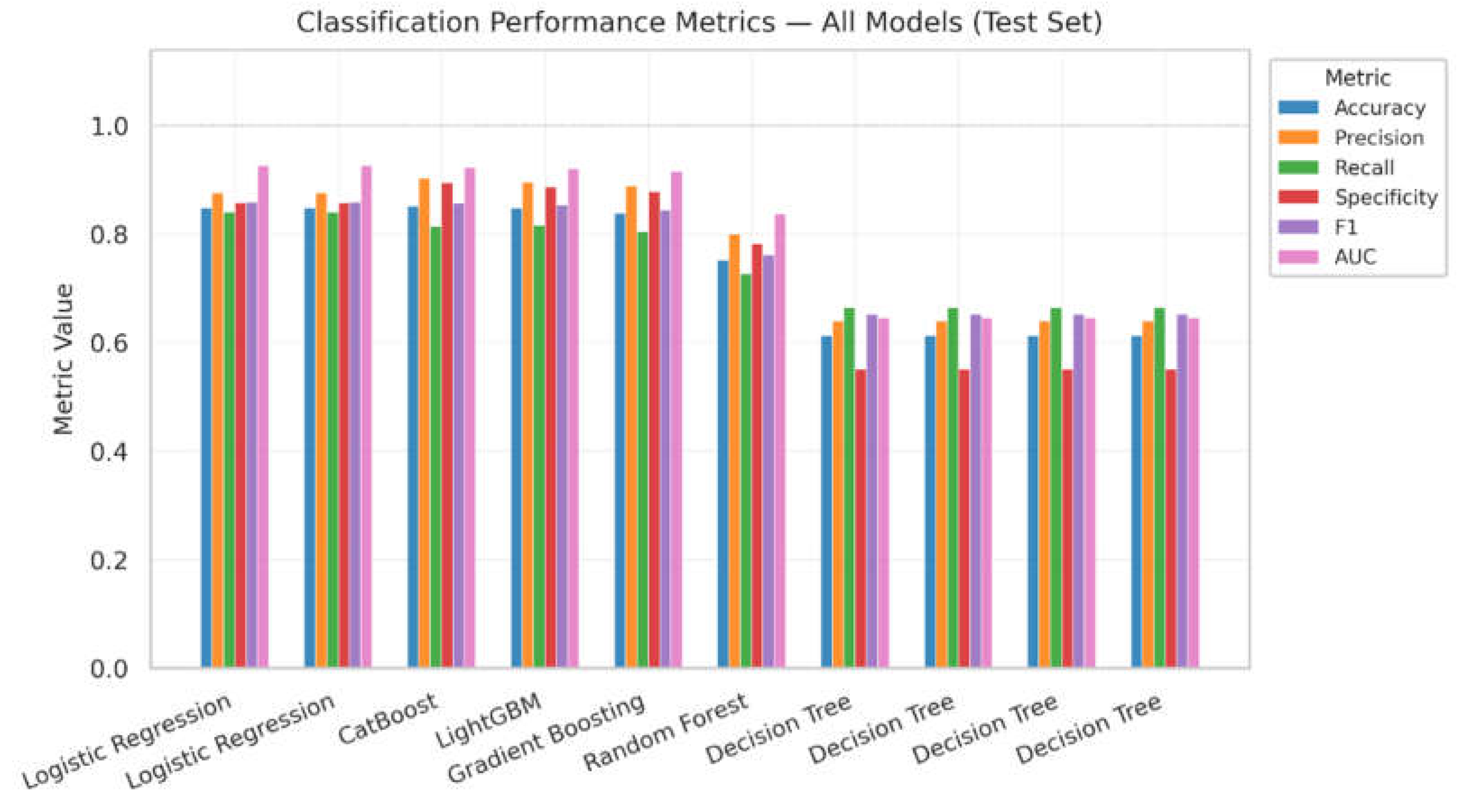
Figure 13.
Precision–Recall curves for all six models. AP: average precision (area under the PR curve). No-skill baseline = 0.546 (class prevalence).
Figure 13.
Precision–Recall curves for all six models. AP: average precision (area under the PR curve). No-skill baseline = 0.546 (class prevalence).
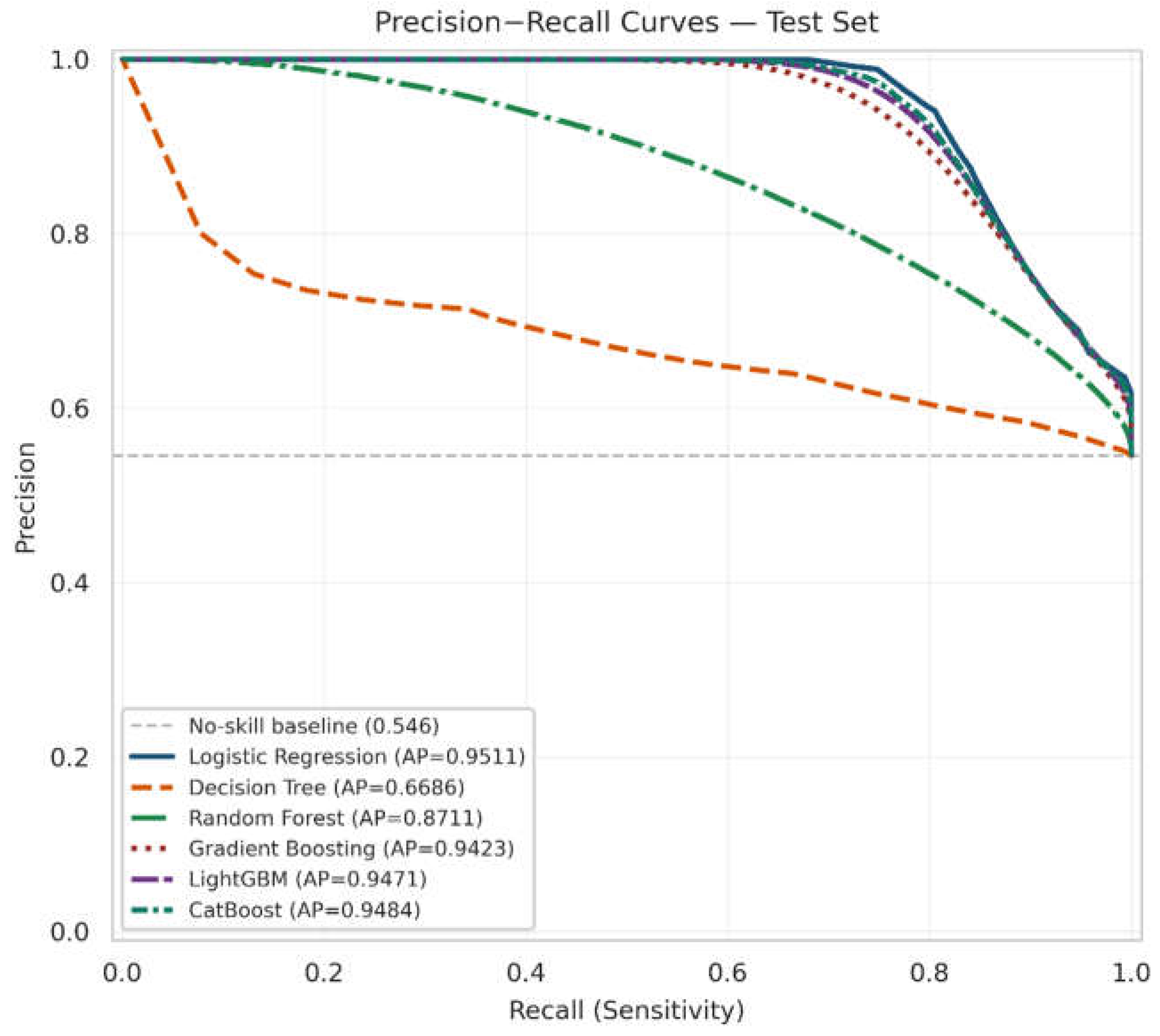
Figure 14.
Reliability diagram for the Logistic Regression classifier on the holdout partition, computed over five equal-frequency bins of predicted probability, centered at approximately 0.03, 0.19, 0.53, 0.89, and 0.99. Dashed diagonal: perfect calibration (holdout Brier score = 0.1067).
Figure 14.
Reliability diagram for the Logistic Regression classifier on the holdout partition, computed over five equal-frequency bins of predicted probability, centered at approximately 0.03, 0.19, 0.53, 0.89, and 0.99. Dashed diagonal: perfect calibration (holdout Brier score = 0.1067).
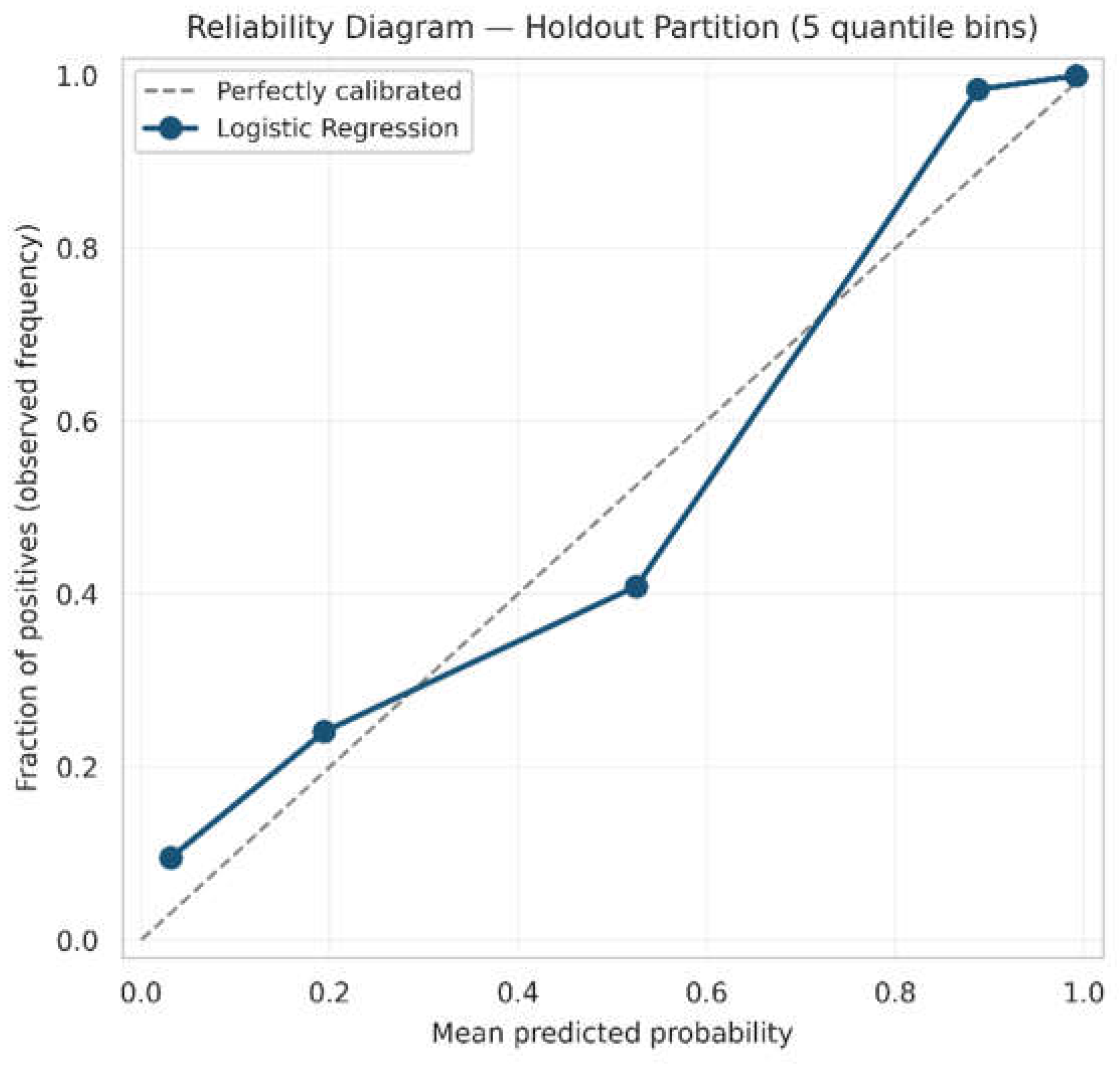
Figure 15.
Log-odds coefficients (β) of Logistic Regression for FloodOccurrence. All positive; horizontal reference at β = 0.
Figure 15.
Log-odds coefficients (β) of Logistic Regression for FloodOccurrence. All positive; horizontal reference at β = 0.
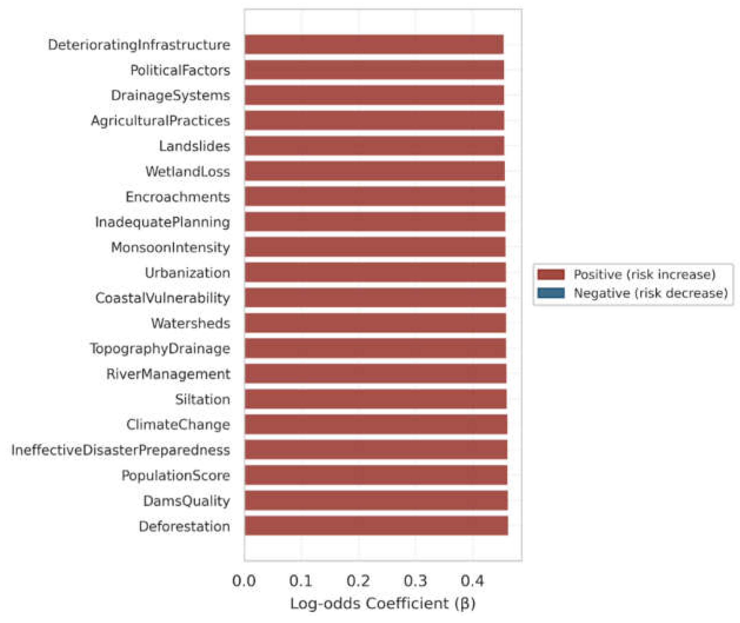
Figure 16.
Confusion matrices for Logistic Regression on training (left) and the holdout partition (right). Accuracy annotated below each matrix.
Figure 16.
Confusion matrices for Logistic Regression on training (left) and the holdout partition (right). Accuracy annotated below each matrix.
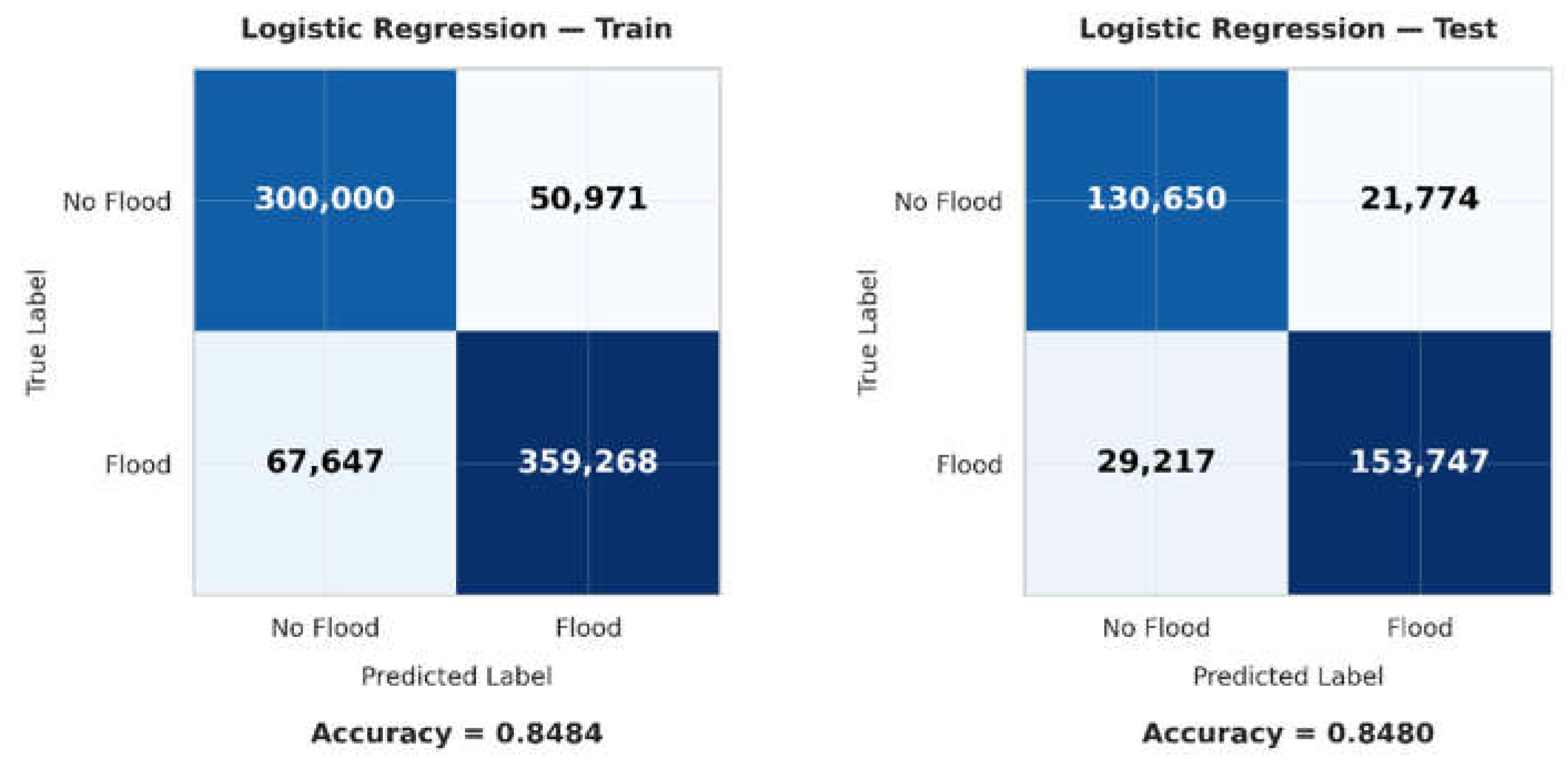
Figure 18.
External verification on flood.csv: (a) predicted vs. observed FloodProbability (n = 5,000 sampled; Pearson r = 0.8979, RMSE = 0.3688); (b) residual plot (MAE = 0.3485).
Figure 18.
External verification on flood.csv: (a) predicted vs. observed FloodProbability (n = 5,000 sampled; Pearson r = 0.8979, RMSE = 0.3688); (b) residual plot (MAE = 0.3485).
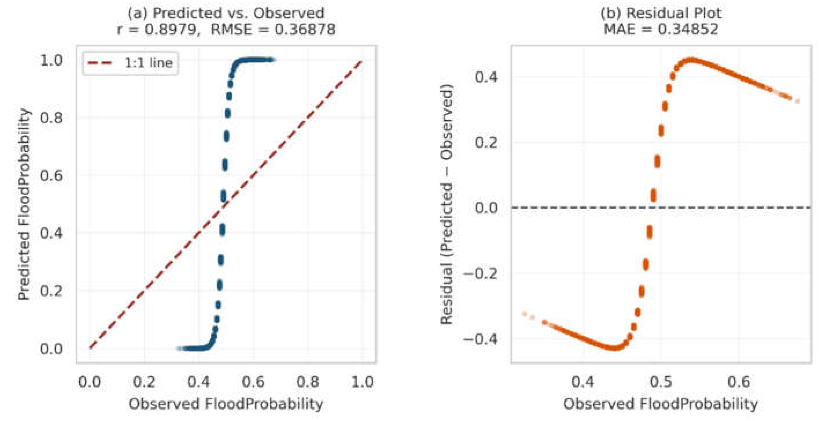
Figure 19.
Classification metrics comparison between the internal holdout partition (train.csv, 30% split) and the external verification subset (flood.csv).
Figure 19.
Classification metrics comparison between the internal holdout partition (train.csv, 30% split) and the external verification subset (flood.csv).
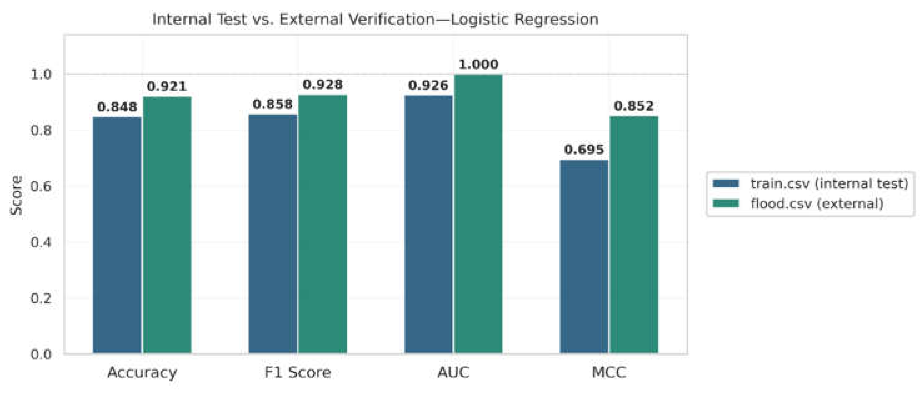
Figure 28.
Discriminative performance across all three scales examined in this study — synthetic, county, and census tract — under both random and spatial evaluation.
Figure 28.
Discriminative performance across all three scales examined in this study — synthetic, county, and census tract — under both random and spatial evaluation.
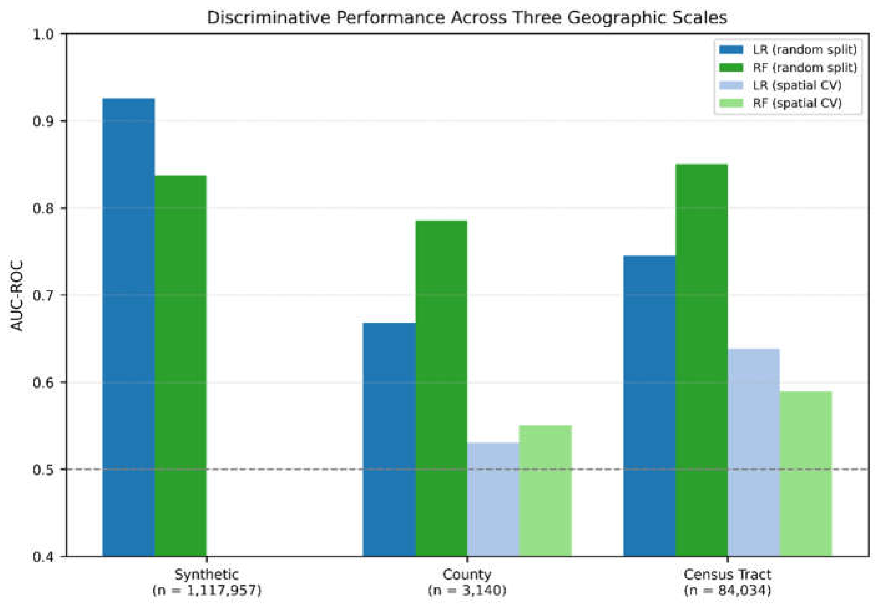
Table 1.
Descriptive statistics of the 20 hydro-environmental predictors and the target variable.
| Mean | SD | Min | 25% |
Median 50% |
75% | Max | Skewness | Kurtosis | CV_% | IQR | Normality (p>0.05) | ||
| Monsoon Intensity | 4.9215 | 2.0564 | 0 | 3 | 5 | 6 | 16 | 0.4445 | 0.3412 | 41.78 | 3 | Non-Normal | |
| Topography Drainage | 4.9267 | 2.0939 | 0 | 3 | 5 | 6 | 18 | 0.4587 | 0.2384 | 42.50 | 3 | Non-Normal | |
| River Management | 4.9553 | 2.0722 | 0 | 4 | 5 | 6 | 16 | 0.4265 | 0.2242 | 41.82 | 2 | Non-Normal | |
| Deforestation | 4.9422 | 2.0517 | 0 | 4 | 5 | 6 | 17 | 0.4343 | 0.2751 | 41.51 | 2 | Non-Normal | |
| Urbanization | 4.9425 | 2.0834 | 0 | 3 | 5 | 6 | 17 | 0.4422 | 0.2483 | 42.15 | 3 | Non-Normal | |
| ClimateChange | 4.9341 | 2.0577 | 0 | 3 | 5 | 6 | 17 | 0.4294 | 0.2413 | 41.70 | 3 | Non-Normal | |
| Dams Quality | 4.9559 | 2.0831 | 0 | 4 | 5 | 6 | 16 | 0.4414 | 0.2621 | 42.03 | 2 | Non-Normal | |
| Siltation | 4.9278 | 2.0660 | 0 | 3 | 5 | 6 | 16 | 0.4492 | 0.2871 | 41.93 | 3 | Non-Normal | |
| Agricultural Practices | 4.9426 | 2.0685 | 0 | 3 | 5 | 6 | 16 | 0.4211 | 0.2141 | 41.85 | 3 | Non-Normal | |
| Encroachments | 4.9492 | 2.0833 | 0 | 4 | 5 | 6 | 18 | 0.4636 | 0.2666 | 42.09 | 2 | Non-Normal | |
| Ineffective Disaster Preparedness | 4.9452 | 2.0781 | 0 | 3 | 5 | 6 | 16 | 0.4434 | 0.2083 | 42.02 | 3 | Non-Normal | |
| Drainage Systems | 4.9469 | 2.0723 | 0 | 4 | 5 | 6 | 17 | 0.4414 | 0.2942 | 41.89 | 2 | Non-Normal | |
| Coastal Vulnerability | 4.9540 | 2.0889 | 0 | 3 | 5 | 6 | 17 | 0.4399 | 0.2390 | 42.17 | 3 | Non-Normal | |
| Landslides | 4.9314 | 2.0783 | 0 | 3 | 5 | 6 | 16 | 0.4251 | 0.1855 | 42.14 | 3 | Non-Normal | |
| Watersheds | 4.9290 | 2.0824 | 0 | 3 | 5 | 6 | 16 | 0.4505 | 0.2377 | 42.25 | 3 | Non-Normal | |
| Deteriorating Infrastructure | 4.9259 | 2.0648 | 0 | 3 | 5 | 6 | 17 | 0.4442 | 0.2473 | 41.92 | 3 | Non-Normal | |
| Population Score | 4.9275 | 2.0742 | 0 | 3 | 5 | 6 | 18 | 0.4514 | 0.2520 | 42.09 | 3 | Non-Normal | |
| Wetland Loss | 4.9509 | 2.0687 | 0 | 4 | 5 | 6 | 19 | 0.4370 | 0.2360 | 41.78 | 2 | Non-Normal | |
| Inadequate Planning | 4.9406 | 2.0811 | 0 | 3 | 5 | 6 | 16 | 0.4551 | 0.2490 | 42.12 | 3 | Non-Normal | |
| Political Factors | 4.9390 | 2.0904 | 0 | 3 | 5 | 6 | 16 | 0.4376 | 0.1989 | 42.32 | 3 | Non-Normal | |
| Flood Probability | 0.5045 | 0.0510 | 0.29 | 0.47 | 0.50 | 0.54 | 0.73 | 0.0472 | –0.0396 | 10.11 | 0.07 | Normal | |
Note: N=1,117,957 for all variables (zero missing values). SD: standard deviation; min/max: minimum and maximum observed values; 25%, 50%, 75%: first, second (median), and third quartiles; IQR: interquartile range (75% − 25%); CV_%: coefficient of variation (%). Skewness and kurtosis quantify distribution asymmetry and tail heaviness, respectively. The 'Normality' column reports the outcome of the D'Agostino–Pearson omnibus test (K²), evaluated on a stratified random subsample (n=5,000) per variable for computational efficiency; 'Normal' denotes p>0.05, and 'Non-Normal' denotes p≤0.05.
Table 2.
Correlation coefficients between the 20 hydro-environmental predictors and FloodProbability.
Table 2.
Correlation coefficients between the 20 hydro-environmental predictors and FloodProbability.
| Pearson_r | Spearman_ρ | |
| Urbanization | 0.1931 | 0.1838 |
| Deteriorating Infrastructure | 0.1912 | 0.1799 |
| Monsoon Intensity | 0.1899 | 0.1794 |
| Landslides | 0.1894 | 0.1814 |
| Inadequate Planning | 0.1880 | 0.1796 |
| River Management | 0.1870 | 0.1771 |
| Dams Quality | 0.1839 | 0.1738 |
| Coastal Vulnerability | 0.1838 | 0.1789 |
| Encroachments | 0.1834 | 0.1740 |
| Agricultural Practices | 0.1832 | 0.1705 |
| Topography Drainage | 0.1829 | 0.1747 |
| Deforestation | 0.1822 | 0.1760 |
| PopulationScore | 0.1822 | 0.1762 |
| Ineffective Disaster Preparedness | 0.1821 | 0.1773 |
| Watersheds | 0.1794 | 0.1723 |
| Wetland Loss | 0.1784 | 0.1728 |
| Climate Change | 0.1779 | 0.1691 |
| Siltation | 0.1778 | 0.1723 |
| Drainage Systems | 0.1755 | 0.1722 |
| Political Factors | 0.1708 | 0.1641 |
Note: N = 1,117,957. Sorted by descending Pearson r. All correlations are highly significant at BH-FDR q < 0.001. Spearman’s ρ is the primary metric given the confirmed non-normality of the predictors.
Table 3.
Multi-metric performance comparison of six machine learning classifiers on the independent holdout partition (n = 335,388). Models sorted by descending AUC-ROC; bold values indicate the best result per column.
Table 3.
Multi-metric performance comparison of six machine learning classifiers on the independent holdout partition (n = 335,388). Models sorted by descending AUC-ROC; bold values indicate the best result per column.
| Model | Acc. | Prec. | Recall | Spec. | F1 | MCC | κ | AUC-ROC |
| Logistic Regression | 0.8480 | 0.8759 | 0.8403 | 0.8571 | 0.8578 | 0.6953 | 0.6946 | 0.9256 |
| CatBoost | 0.8509 | 0.9029 | 0.8143 | 0.8949 | 0.8563 | 0.7063 | 0.7023 | 0.9222 |
| LightGBM | 0.8474 | 0.8958 | 0.8151 | 0.8862 | 0.8536 | 0.6984 | 0.6950 | 0.9207 |
| Gradient Boosting | 0.8381 | 0.8882 | 0.8046 | 0.8784 | 0.8443 | 0.6802 | 0.6766 | 0.9150 |
| Random Forest | 0.7516 | 0.7995 | 0.7270 | 0.7811 | 0.7615 | 0.5060 | 0.5035 | 0.8372 |
| Decision Tree | 0.6127 | 0.6395 | 0.6645 | 0.5504 | 0.6518 | 0.2160 | 0.2158 | 0.6456 |
Note: Acc.: Accuracy; Prec.: Precision; Spec.: Specificity; MCC: Matthews Correlation Coefficient; κ: Cohen's Kappa; AUC-ROC: Area Under Receiver Operating Characteristic Curve. Best value per column in bold.
Table 4.
Probability calibration summary for the best-performing classifier (Logistic Regression).
| Partition | n | Brier Score | Brier Score (Platt-scaled) | Relative Improvement |
| Holdout (train.csv, 30% split) | 335388 | 0.1067 | 0.1089 | +2.1% (worse) |
| External verification (flood.csv) | 50000 | 0.0455 | n/a | n/a |
Note: Platt scaling was fitted and evaluated on the holdout partition only; it was not applied to the external subset. A positive relative change indicates a higher (worse) Brier score after recalibration.
Table 5.
Threshold-sensitivity analysis for the Logistic Regression classifier on the holdout partition (n = 335,388).
Table 5.
Threshold-sensitivity analysis for the Logistic Regression classifier on the holdout partition (n = 335,388).
| Threshold | Accuracy | Precision | Recall | F1 |
| 0.1 | 0.7212 | 0.6722 | 0.9545 | 0.7889 |
| 0.2 | 0.7618 | 0.7204 | 0.9208 | 0.8084 |
| 0.3 | 0.7843 | 0.7527 | 0.9004 | 0.8200 |
| 0.4 | 0.8116 | 0.7980 | 0.8765 | 0.8354 |
| 0.5 | 0.8480 | 0.8759 | 0.8403 | 0.8578 |
| 0.6 | 0.8662 | 0.9409 | 0.8053 | 0.8679 |
| 0.7 | 0.8579 | 0.9883 | 0.7484 | 0.8518 |
| 0.8 | 0.8247 | 0.9996 | 0.6789 | 0.8086 |
| 0.9 | 0.7716 | 0.9996 | 0.5814 | 0.7352 |
F1 peaks at threshold = 0.60. Precision plateaus near 0.9996 from threshold >= 0.80, indicating almost no false alarms remain at that range, at a substantial cost in recall.
Table 6.
Logistic Regression log-odds coefficients (β) and odds ratios (OR = exp(β)) for all 20 predictors, fitted on balanced calibration set, (n = 853,830 after Random Oversampling). Sorted by descending β.
Table 6.
Logistic Regression log-odds coefficients (β) and odds ratios (OR = exp(β)) for all 20 predictors, fitted on balanced calibration set, (n = 853,830 after Random Oversampling). Sorted by descending β.
| Variable | Beta |
Odds_Ratio OR = exp(β) |
Rank |
| Deforestation | 0.46220 | 1.58756 | 1 |
| DamsQuality | 0.46166 | 1.58671 | 2 |
| PopulationScore | 0.46113 | 1.58586 | 3 |
| IneffectiveDisasterPreparedness | 0.46093 | 1.58555 | 4 |
| ClimateChange | 0.46073 | 1.58522 | 5 |
| Siltation | 0.45957 | 1.58339 | 6 |
| RiverManagement | 0.45927 | 1.58292 | 7 |
| TopographyDrainage | 0.45893 | 1.58237 | 8 |
| Watersheds | 0.45881 | 1.58220 | 9 |
| CoastalVulnerability | 0.45877 | 1.58212 | 10 |
| Urbanization | 0.45804 | 1.58097 | 11 |
| MonsoonIntensity | 0.45786 | 1.58069 | 12 |
| InadequatePlanning | 0.45693 | 1.57923 | 13 |
| Encroachments | 0.45692 | 1.57920 | 14 |
| WetlandLoss | 0.45592 | 1.57763 | 15 |
| Landslides | 0.45561 | 1.57714 | 16 |
| AgriculturalPractices | 0.45541 | 1.57683 | 17 |
| DrainageSystems | 0.45507 | 1.57629 | 18 |
| PoliticalFactors | 0.45479 | 1.57584 | 19 |
| DeterioratingInfrastructure | 0.45467 | 1.57565 | 20 |
OR: odds ratio. Coefficient range (max-min) = 0.0075 (1.6% of the maximum value).
Table 7.
5-fold stratified cross-validation results for the three best-performing classifiers. 95% CIs computed as mean ± 1.96 × SD.
Table 7.
5-fold stratified cross-validation results for the three best-performing classifiers. 95% CIs computed as mean ± 1.96 × SD.
| Model | Metric | Mean | SD | Min | Max | 95% CI |
| Logistic Regression | Accuracy | 0.8484 | 0.0007 | 0.8475 | 0.8496 | [0.8470, 0.8498] |
| Logistic Regression | F1 | 0.8583 | 0.0006 | 0.8577 | 0.8594 | [0.8572, 0.8595] |
| Logistic Regression | AUC | 0.9257 | 0.0004 | 0.9253 | 0.9264 | [0.9250, 0.9265] |
| CatBoost | Accuracy | 0.8382 | 0.0009 | 0.8370 | 0.8393 | [0.8365, 0.8399] |
| CatBoost | F1 | 0.8502 | 0.0007 | 0.8493 | 0.8511 | [0.8489, 0.8514] |
| CatBoost | AUC | 0.9224 | 0.0004 | 0.9220 | 0.9231 | [0.9216, 0.9231] |
| LightGBM | Accuracy | 0.8373 | 0.0010 | 0.8358 | 0.8386 | [0.8353, 0.8393] |
| LightGBM | F1 | 0.8494 | 0.0007 | 0.8483 | 0.8504 | [0.8479, 0.8508] |
| LightGBM | AUC | 0.9207 | 0.0004 | 0.9204 | 0.9213 | [0.9200, 0.9213] |
Note: CI, confidence interval; SD: standard deviation. Mean ± SD; 95% CI computed as mean ± 1.96 × SD across the five fold-level scores. Metrics evaluated on the calibration partition n = 782,569 (original class distribution, prior to Random Oversampling) for each fold.
Table 8.
External verification metrics of the Logistic Regression model on the flood.csv subset (n = 50,000).
Table 8.
External verification metrics of the Logistic Regression model on the flood.csv subset (n = 50,000).
| Metric | Value |
| Accuracy | 0.9208 |
| F1-score | 0.9280 |
| AUC-ROC | 1.0000 * |
| Matthews Correlation Coefficient (MCC) | 0.8519 |
| Cohen's Kappa (κ) | 0.8411 |
| Pearson r (continuous probability) | 0.8979 |
| Spearman ρ (continuous probability) | 0.9995 |
| RMSE (continuous probability) | 0.3688 |
| MAE (continuous probability) | 0.3485 |
| Brier Score (continuous probability) | 0.0455 |
Note: RMSE: Root Mean Square Error; MAE: Mean Absolute Error. * AUC = 1.0000 reflects distributional overlap with training corpus rather than operational forecasting skill (Section 3.8, Section 4.4). Classification metrics are evaluated at the 0.5 threshold; continuous-probability metrics against the ground-truth FloodProbability values.
Table 9.
Stage II (FEMA NRI, county) holdout performance, n = 942 counties. Sorted by descending AUC-ROC.
Table 9.
Stage II (FEMA NRI, county) holdout performance, n = 942 counties. Sorted by descending AUC-ROC.
| Model | Acc. | Prec. | Recall | F1 | MCC | AUC-ROC | Brier |
| Random Forest | 0.7389 | 0.6894 | 0.6033 | 0.6435 | 0.4413 | 0.7855 | 0.1841 |
| CatBoost | 0.7293 | 0.6548 | 0.6495 | 0.6521 | 0.4306 | 0.7825 | 0.1866 |
| LightGBM | 0.7473 | 0.6868 | 0.6495 | 0.6676 | 0.4646 | 0.7853 | 0.1872 |
| Gradient Boosting | 0.7134 | 0.6392 | 0.6114 | 0.6250 | 0.3935 | 0.7635 | 0.1946 |
| Logistic Regression | 0.6051 | 0.4960 | 0.6793 | 0.5734 | 0.2317 | 0.6680 | 0.2288 |
| Decision Tree | 0.6624 | 0.5698 | 0.5543 | 0.5620 | 0.2875 | 0.6665 | 0.2353 |
Table 12.
Prevalence of high inland-flood historic-loss-ratio rating by U.S. Census region.
| Census region | n counties | FloodRiskHigh prevalence |
| Midwest | 1055 | 0.5611 |
| Northeast | 218 | 0.2706 |
| South | 1422 | 0.2679 |
| West | 445 | 0.4360 |
Table 13.
Stage III (FEMA NRI, census tract) holdout performance, n = 25,211 tracts. Sorted by descending AUC-ROC.
Table 13.
Stage III (FEMA NRI, census tract) holdout performance, n = 25,211 tracts. Sorted by descending AUC-ROC.
| Model | Acc. | Prec. | Recall | F1 | MCC | AUC-ROC | Brier |
| Random Forest | 0.8188 | 0.6742 | 0.5717 | 0.6188 | 0.5039 | 0.8507 | 0.1295 |
| LightGBM | 0.7851 | 0.5676 | 0.6911 | 0.6233 | 0.4795 | 0.8416 | 0.1506 |
| CatBoost | 0.7733 | 0.5464 | 0.6979 | 0.6129 | 0.4628 | 0.8336 | 0.1606 |
| Gradient Boosting | 0.7686 | 0.5397 | 0.6818 | 0.6025 | 0.4484 | 0.8224 | 0.1654 |
| Decision Tree | 0.7166 | 0.4622 | 0.6243 | 0.5312 | 0.3422 | 0.7503 | 0.1931 |
| Logistic Regression | 0.6955 | 0.4371 | 0.6396 | 0.5193 | 0.3197 | 0.7449 | 0.1994 |
Table 16.
Master comparison across all three stages of this study. "n/a" reflects the absence of verifiable geography in the synthetic benchmark, which precludes any spatial cross-validation design.
Table 16.
Master comparison across all three stages of this study. "n/a" reflects the absence of verifiable geography in the synthetic benchmark, which precludes any spatial cross-validation design.
| Scale | n (analytic sample) | AUC LR (random) | AUC RF (random) | AUC LR (spatial) | AUC RF (spatial) |
| Synthetic | 1,117,957 | 0.9256 | 0.8372 | n/a | n/a |
| County | 3,140 | 0.6680 | 0.7855 | 0.5306 | 0.5501 |
| Census Tract | 84,034 | 0.7449 | 0.8507 | 0.6384 | 0.5897 |
Disclaimer/Publisher’s Note: The statements, opinions and data contained in all publications are solely those of the individual author(s) and contributor(s) and not of MDPI and/or the editor(s). MDPI and/or the editor(s) disclaim responsibility for any injury to people or property resulting from any ideas, methods, instructions or products referred to in the content. |
© 2026 by the authors. Licensee MDPI, Basel, Switzerland. This article is an open access article distributed under the terms and conditions of the Creative Commons Attribution (CC BY) license (http://creativecommons.org/licenses/by/4.0/).
Copyright: This open access article is published under a Creative Commons CC BY 4.0 license, which permit the free download, distribution, and reuse, provided that the author and preprint are cited in any reuse.


