

Submitted:
07 August 2026
Posted:
07 August 2026
You are already at the latest version
Abstract
Non-destructive in-situ tests, such as the plate bearing (plate load) test, are widely used to estimate the equivalent deformation modulus (e.g., Ev2) of existing road embankments. However, the depth of influence sampled by such a test is governed by the loading plate diameter, so a single test yields only an average, diameter-dependent modulus rather than the actual variation of stiffness with depth. This study investigates whether systematically varying the plate diameter, and inverting the resulting settlement–diameter (dispersion) curves, can recover the full depth-dependent stiffness profile, E(z). Synthetic settlement–diameter curves were generated using a Boussinesq-based forward model for four families of reference stiffness profiles, representing normal (stiffness increasing with depth) and reverse (stiffness decreasing with depth) linear and exponential trends, combined with six Poisson’s ratios and five profile slopes/exponents (30 cases per profile family, 120 cases in total). Two inversion strategies were applied to back-calculate E(z) from each dispersion curve: a classical Occam-type, smoothness-constrained (Tikhonov-regularized) nonlinear inversion, and a direct, closed-form Simplified Inversion Method (SIM) based on differencing the apparent-modulus-versus-diameter curve. Results were benchmarked against the known reference profiles. Once calibrated so that its governing parameters depend only on Poisson’s ratio and the shape of the measured dispersion curve, SIM could be applied blindly, without prior knowledge of the true profile, and recovered E(z) with markedly lower error than Occam’s inversion (WAD = 2.2–4.7% and RMSPE = 2.6–5.8%, versus 7.4–19.1% and 9.4–28.3%, respectively, across the four profile families). For the Poisson’s ratio most typical of earth materials, ν = 0.3, the calibration further collapses to a universal parameter set (I = 0.66; c = 1.3 for stiffness increasing with depth, c = 2.5 for stiffness decreasing with depth), which attains WAD ≤ 4.2% across all four families with no calibration equation at all. Notably, Occam’s inversion reproduced the settlement–diameter curve itself with good accuracy in most cases, yet this close data fit did not guarantee an accurate stiffness profile—a direct manifestation of the intrinsic non-uniqueness of the settlement-based inverse problem. These findings support the use of a Poisson ratio-calibrated direct inversion method as a practical, robust alternative to generic regularized inversion for recovering stiffness profiles from multi-diameter plate loading data.
Keywords:
plate load test
; embankment characterization
; non-destructive testing
; inverse analysis
; Occam’s inversion
; non-uniqueness
; soil stiffness profile
1. Introduction
The assessment of the mechanical condition of existing road embankments and earthworks is a recurring task in transportation geotechnics, particularly in the context of pavement rehabilitation, widening projects, and the re-evaluation of aging infrastructure. Because intrusive sampling of a compacted embankment is costly, disruptive to traffic, and often unrepresentative of the in-place condition, practice relies heavily on non-destructive in-situ testing. Among the available methods, the static plate bearing (plate load) test occupies a central position: it is standardized (e.g., ASTM D1195/D1195M [2] and DIN 18134 [1]), directly measures a load–settlement response under conditions resembling those imposed by traffic and foundation loads, and yields the widely used strain moduli and that serve as acceptance criteria in earthworks specifications across Europe.
Notwithstanding its popularity, the plate bearing test suffers from a fundamental interpretive limitation. The settlement of a loaded circular plate reflects the deformation of a volume of soil whose depth of influence scales with the plate diameter D—commonly taken as roughly 1.5–2D below the loaded surface. Consequently, the deformation modulus back-figured from a single test is not a soil property at a specific depth but a weighted average over the influence volume, with the weighting dictated by the elastic stress distribution beneath the plate. Two embankments with markedly different stiffness–depth profiles can therefore return identical values for a given plate size, and, conversely, the same embankment tested with different plate diameters will generally return different moduli [3].
This diameter dependence, usually regarded as a nuisance, can instead be exploited as a source of information. If the plate diameter is varied systematically and the corresponding settlements are recorded under a common contact pressure, the resulting settlement–diameter curve, —referred to here as a dispersion curve, by direct analogy with the frequency- (wavelength-) dependent phase-velocity curves of surface-wave testing—encodes the variation of soil stiffness with depth: small plates predominantly sample the shallow material, whereas large plates engage progressively deeper strata. Recovering the modulus profile from is then an inverse problem with the same mathematical structure as the inversion of surface-wave dispersion curves for the shear-wave velocity profile [4] or the backcalculation of pavement layer moduli from falling-weight deflectometer (FWD) deflection basins [7,8]: a smooth, integrating forward operator maps a stiffness–depth function onto a small set of surface observations, rendering the inverse mapping ill-posed and non-unique.
In the geophysical literature, the reference approach to such ill-posed problems is Occam’s inversion, introduced by Constable, Parker and Constable [9] and extended to two dimensions by DeGroot-Hedlin and Constable [10]. Building on Tikhonov regularization [11], Occam’s inversion seeks the smoothest model—in the sense of a minimum-roughness penalty—that reproduces the observations to within a prescribed tolerance, with the trade-off between data misfit and model roughness controlled by a regularization parameter . The approach is deliberately conservative: by returning the smoothest acceptable model, it avoids overinterpreting features that the data cannot resolve. Its limitations are, however, equally well documented. The inverse problem remains fundamentally non-unique, so that many stiffness distributions reproduce the data essentially equally well; the smoothness constraint blurs sharp stiffness contrasts and can produce Gibbs-type overshoot at layer boundaries [12,13]; resolution decays rapidly with depth as the sensitivity of the surface observations to deep model parameters vanishes; and the selection of the regularization parameter—whether by the L-curve criterion [14], generalized cross-validation [15], or related statistical criteria [16]—is itself delicate, with the L-curve method provably failing to converge to the correct parameter as the data noise tends to zero [17]. These weaknesses have motivated a rich literature of alternatives, including sparsity-promoting and focusing regularization [12], transdimensional Bayesian formulations [4,18], and global optimization schemes [19], none of which, however, removes the underlying non-uniqueness; they either reshape the prior or quantify the resulting uncertainty.
In geotechnical engineering, by contrast, regularized inversion of plate settlement data for a continuous modulus profile has received little attention. Elastic solutions for non-homogeneous media—notably Gibson’s linearly increasing modulus half-space [20], its finite-layer extension [21], and related non-homogeneous formulations [22]—provide the forward-modelling ingredients, and displacement influence factors for foundations on such media are well established [3]. Inverse analyses of plate load tests have generally targeted a small number of layer parameters through direct optimization [23] rather than a full profile through regularized inversion.
The present study addresses this gap through a systematic synthetic benchmarking exercise with three objectives: (i) to assess whether the multi-diameter plate bearing test can, in principle, recover depth-dependent stiffness profiles representative of road embankments; (ii) to present and calibrate a direct, closed-form Simplified Inversion Method (SIM)—the counterpart, for plate loading data, of the simplified inversion method previously proposed and validated by the first author for surface-wave (Rayleigh-wave) dispersion curves [5,6]—whose two governing parameters are shown to depend only on Poisson’s ratio and a single shape descriptor of the measured dispersion curve, so that the method can subsequently be applied blindly; and (iii) to compare SIM against a state-of-practice Occam-type regularized inversion over 120 synthetic cases spanning four profile families, six Poisson’s ratios and five profile slopes. Particular attention is paid to a phenomenon that emerges consistently from the comparison and gives the paper its title: Occam’s inversion frequently reproduces the settlement–diameter curve with high accuracy while returning a substantially incorrect stiffness profile, providing a concrete, geotechnically relevant illustration of the non-uniqueness of the settlement-based inverse problem.
The paper is organized as follows. Section 2 describes the common forward model and the two inversion methods. Section 3 details the synthetic database, the SIM calibration procedure, and the Occam application protocol. Section 4 presents the results, Section 5 discusses their implications and limitations, and Section 6 summarizes the conclusions.
2. Inversion Methods
2.1. Forward Model
Both inversion methods considered here rest on the same forward model, which computes the surface settlement of a uniformly loaded circular plate resting on a layered elastic medium. Following the classical strain-influence formulation, the vertical strain at depth z beneath the centre of a circular area of radius carrying a uniform contact pressure q is expressed through the Boussinesq stress solution as
where is the Young’s modulus at depth z, is the Poisson’s ratio and is the strain influence factor,
with and the Boussinesq vertical and radial stress increments beneath the centre of the loaded area. For a medium discretized into N horizontal layers of constant modulus , bounded by depths and , the surface settlement follows by summation of the layer compressions:
where the leading coefficient is the rigid-plate factor, adopted throughout this study as consistent with the steel plates used in practice; a perfectly flexible plate would instead carry a factor of unity. The integral in Equation (3) is evaluated numerically, and the deepest layer is treated as a half-space by extending the integration to an effectively infinite depth.
Equation (3) makes the physical origin of the inverse problem’s difficulty explicit: the settlement is a weighted integral of the soil compliance , with a smooth, slowly decaying kernel . The forward operator therefore acts as a low-pass filter on the stiffness profile, and profiles differing by oscillatory or deep-seated components that the kernel suppresses map onto nearly identical settlement curves.
A convenient derived quantity is the apparent modulus associated with each plate diameter,
where I is a dimensionless influence coefficient. Equation (4) is the standard elastic settlement formula solved for the modulus; for a homogeneous half-space, is independent of D, whereas any diameter dependence of directly reflects the depth variation of stiffness. The curve is therefore an equivalent, and often more interpretable, representation of the dispersion curve .
A distinction is drawn throughout between two uses of Equation (4). The nominal apparent-modulus curve is obtained by fixing , i.e. ; it requires no prior information beyond the raw measurements and is the curve plotted, reported, and used in Section 3.5 to characterize the shape of the dispersion data. The calibrated apparent modulus, in which I takes its case-specific calibrated value, is instead used only internally, within the SIM inversion of Section 2.3, to recover the stiffness profile itself. This separation ensures that the shape descriptor of the dispersion curve is available directly from the measurements, before—and independently of—the calibrated influence coefficient.
2.2. Occam’S Smoothness-Constrained Inversion
The regularized inversion follows the Occam philosophy of Constable et al. [9], adapted to the plate settlement problem. The model vector collects the logarithms of the layer moduli, , which enforces positivity of the recovered moduli and reduces the nonlinearity of the forward map. The medium is discretized into layers, where M is the number of plate diameters (observations): the upper M layer boundaries are placed at depths proportional to the tested diameters, with c the representative-depth ratio defined in Section 2.3, and the final layer, of prescribed thickness, represents the underlying half-space.
At each Gauss–Newton iteration, the model update is obtained from the regularized normal equations
where is the Jacobian of the forward model with respect to , evaluated by finite differences; is the residual vector between observed and computed settlements; weights the residuals by the reciprocal of the observed settlements, so that all diameters contribute comparable relative errors; and is the first-order finite-difference operator acting on adjacent layers, so that the penalty term measures the roughness of the log-modulus profile. The regularization parameter is normalized through
which renders the nominal dimensionless and transferable across cases of different scale. Model updates are limited to per iteration to stabilize the iteration, and the scheme terminates when the relative step norm falls below or after a maximum of 40 iterations.
For each case, the inversion is repeated over a logarithmic sweep of the regularization parameter, , discretized in steps of decades. The operating value of is then selected automatically at the corner of the L-curve—the parametric curve of log data-misfit against log model-roughness—identified as the point of maximum curvature [14]. The selection is entirely blind: it uses only the misfit–roughness trade-off and has no access to the reference profile. The initial model is a uniform profile at the mean apparent modulus of the measured curve.
It is emphasized that this implementation incorporates the standard good practice of the regularized-inversion literature—logarithmic model parameters, relative data weighting, trace-normalized regularization, convergence-controlled iterations, and curvature-based L-curve selection—so that the comparison of Section 4 confronts SIM with a properly configured, rather than a deliberately weakened, Occam inversion.
2.3. the Simplified Inversion Method (SIM)
The Simplified Inversion Method takes the opposite route: instead of regularizing a general many-parameter model, it postulates a compact, physically motivated construction with only two free parameters and inverts the dispersion curve directly, without iteration.
The method proceeds in three steps. First, the measured dispersion curve is converted to apparent moduli through Equation (4), using the calibrated influence coefficient I—evaluated, as described in Section 3.5, from the Poisson’s ratio and the shape descriptor of the nominal () dispersion curve—rather than the nominal value used only to characterize the raw data. Second, each apparent modulus , for diameters ordered , is assigned to a representative depth
where the depth ratio c is the second calibration parameter: it expresses the depth at which the average modulus sensed by a plate of diameter is best localized, in the spirit of characteristic-depth arguments used in surface-wave processing. The two calibrated parameters, I and c, are thus applied together, at this single inversion step, on the same footing.
Write for the nominal () apparent modulus of Equation (4) at . Both differencing variants share an identical peeling structure, applied to a calibrated nodal quantity and its local secant slope,
but differ in what represents and in whether the peeled value is taken directly as the local modulus or inverted to yield it. For reverse profiles (decreasing , Profile Families 2 and 4), is the calibrated apparent modulus itself, and the peeled value is used directly,
For normal profiles (increasing , Profile Families 1 and 3), is instead the calibrated apparent compliance—the natural variable of Equation (3)—and the peeled value is inverted to recover the modulus,
In either case the shallowest layer requires no peeling, since removes the second term of Equation (8):
The two variants thus share the identical peeling operation of Equation (8); they differ only in the definition of and in the final direct-or-inverse step, with no additional quantity introduced. Because this peeling is carried out in the diameter domain D rather than the depth domain , the depth-calibration parameter c enters only afterward, through , at which each peeled node is subsequently plotted—so that I and c act independently within the same inversion step, I rescaling the peeled node values and c relocating them in depth. The variant is selected from the sign of the slope of the nominal dispersion curve, i.e. directly from the profile family; this rule reproduces the variant found to perform best in the exhaustive per-case comparison of Section 3.4. The recovered profile is therefore a piecewise-constant (step) function of depth,
consistent with the layered discretization also used by Occam’s inversion (Section 2.2).
Figure 1.
Schematic illustration of the application of SIM to an –D dispersion curve, as obtained from plate load test results.
Figure 1.
Schematic illustration of the application of SIM to an –D dispersion curve, as obtained from plate load test results.
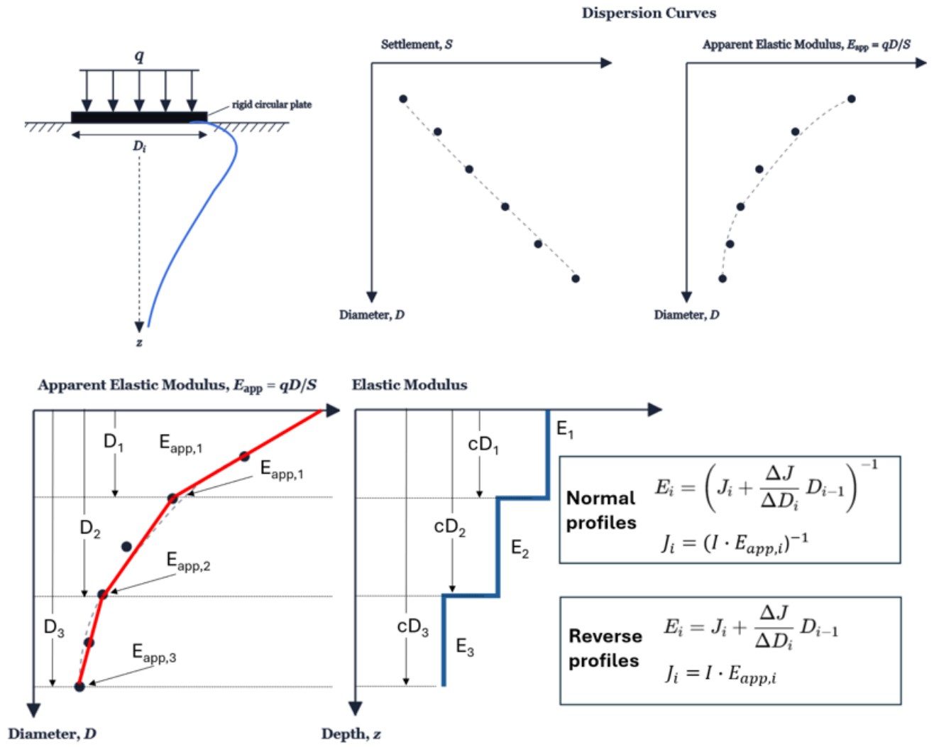
The construction is deliberately analogous to classical direct interpretation schemes of near-surface geophysics, in which a cumulative sounding curve is differentiated with respect to an abscissa playing the role of depth in order to localize layer properties. In particular, it transfers to plate loading data the simplified inversion method developed by the first author for surface-wave (Rayleigh-wave) dispersion curves [5,6]: there, apparent phase velocities are assigned to equivalent penetration depths proportional to the wavelength () and peeled layer by layer through relations formally identical to Equations (9) and (10), and the approach has been validated extensively against advanced iterative inversion schemes on both synthetic and field data. Its decisive feature is that the entire inversion is expressed in closed form: no Jacobian, no iteration, no regularization parameter and no starting model are required. All the flexibility of the method is concentrated in the pair , and Section 3.5 shows that this pair can be calibrated once, per profile family, as a smooth function of the Poisson’s ratio and of a single shape descriptor of the dispersion curve—after which SIM operates blindly on measured data.
3. Methodology
3.1. Reference Stiffness Profiles and Synthetic Database
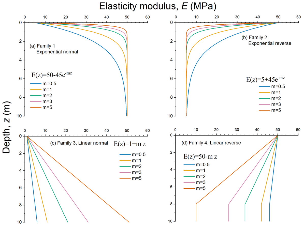
Four families of reference stiffness profiles were considered, chosen to span the depth-variation patterns most commonly encountered in compacted embankments and their foundations. Throughout the paper, profiles in which stiffness increases with depth are termed normal, and profiles in which stiffness decreases with depth are termed reverse. The four families are:
- Profile Family 1 — exponential normal: (MPa), rising from 5 MPa at the surface towards an asymptote of 50 MPa at depth;
- Profile Family 2 — exponential reverse: (MPa), decaying from 50 MPa at the surface towards 5 MPa at depth, representative of a stiff compacted crust over softer material;
- Profile Family 3 — linear normal: (MPa), a Gibson-type linearly increasing profile [20], capped at m;
- Profile Family 4 — linear reverse: (MPa) with negative slope m, capped at m, representing a stiff embankment overlying progressively softer ground.
Each family was evaluated for five values of the slope/exponent parameter and six Poisson’s ratios, , producing 30 cases per family and 120 synthetic cases in total.
Figure 2.
The four families of reference stiffness profiles used in the synthetic study: (a) Profile Family 1, exponential normal; (b) Profile Family 2, exponential reverse; (c) Profile Family 3, linear normal; (d) Profile Family 4, linear reverse. Each panel shows the five profile slopes/exponents considered.
Figure 2.
The four families of reference stiffness profiles used in the synthetic study: (a) Profile Family 1, exponential normal; (b) Profile Family 2, exponential reverse; (c) Profile Family 3, linear normal; (d) Profile Family 4, linear reverse. Each panel shows the five profile slopes/exponents considered.
3.2. Generation of Synthetic Dispersion Curves
For every case, the settlement–diameter curve was computed with the forward model of Section 2.1, using a fine vertical discretization of the continuous reference profile, a common contact pressure kPa, the rigid-plate factor , and a set of 10 plate diameters, m. The resulting synthetic curves are noise-free. This choice is deliberate: it isolates the intrinsic, structural non-uniqueness of the inverse problem from the additional variance introduced by measurement error, and thus represents the most favourable possible conditions for any inversion method. The implications of the noise-free setting for the automatic selection of the regularization parameter in Occam’s inversion are examined in Section 5.
The complete synthetic database is shown in Figure 3: for each profile family, the left panels collect the settlement–diameter curves and the right panels the corresponding nominal apparent-modulus curves , with the plate diameter on the vertical axis, increasing downward, to underline the analogy with depth profiles. All 30 curves of each family—the full grid of five profile parameters m and six Poisson’s ratios —are superimposed in a single uniform tone, deliberately without individual identification: the purpose of the figure is to convey the variety of dispersion responses that a single functional family generates as vary, which is precisely the variability that the shape descriptor and the calibrated pair must absorb. The spread is substantial in both coordinates: within a family the settlements at a given diameter span up to an order of magnitude, and the apparent-modulus curves fan out accordingly. The qualitative signature of each family is nevertheless preserved across its entire grid—apparent moduli increasing with diameter for the normal families (1 and 3), decreasing for the reverse families (2 and 4)—which is what makes the classification of the profile family from the shape of a measured curve, required by the blind protocol, feasible in the first place.
3.3. Error Metrics
The accuracy of a recovered profile relative to the reference is quantified by two depth-integrated, pointwise-normalized measures: the weighted absolute deviation,
and the root-mean-square percentage error,
Both metrics normalize the error pointwise by the local reference modulus before integrating over depth. This is essential in the present context, where the reference moduli span an order of magnitude within a single profile: an absolute (MPa-valued) RMSE would implicitly weight the stiff portions of the profile far more heavily than the soft ones, biasing both the calibration and the comparison. WAD, an -type measure, characterizes the average relative deviation and is comparatively insensitive to localized outliers; RMSPE, its counterpart, penalizes concentrated large deviations more severely. Reporting both jointly is deliberately diagnostic: close agreement between WAD and RMSPE indicates a diffuse, evenly distributed error, whereas an RMSPE substantially exceeding the WAD reveals error concentrated over a narrow depth range. In addition, the quality with which each recovered profile reproduces the data themselves is quantified by the RMSPE between the measured settlements and those recomputed from the recovered profile through the forward model, denoted .
3.4. SIM Optimal Parameter Identification
For each of the 120 cases, the optimal SIM parameter pair was identified by exhaustive grid search over and , minimizing the profile error of Equations (13) and (14); the search was performed independently for the two metrics, and for both the direct and inverse differencing variants, retaining the better variant per case. Because WAD and RMSPE weight the depth-distribution of error differently, their optima do not coincide exactly; both optima are recorded, and the internal consistency of the calibration is preserved by always pairing a reported error metric with parameters optimized under that same metric.
The landscapes of Figure 4 exhibit, in every panel, a single global minimum and no secondary minima, so that the two-parameter identification is well-posed and the grid search cannot be trapped away from the optimum. The shape of the low-error region, however, differs markedly and systematically between families, and is diagnostic of how tightly the data constrain each parameter. For Profile Family 1, the minimum lies in a valley elongated along the c-axis: the influence coefficient I is sharply resolved, whereas moderate departures of c from the optimum carry little error penalty. For Profile Family 2, the minimum is a compact, well-localized ellipse centred at a distinctly larger depth ratio (), consistent with the deeper representative depths required when a stiff crust forces the informative deformation to accumulate in the underlying soft material. Profile Family 3 displays a narrow, steeply inclined valley, revealing a strong positive coupling between I and c: along the valley, an increase in c can be almost exactly compensated by an increase in I, a direct consequence of the scale-free character of the linear (Gibson-type) profile, for which the data constrain a combination of the two parameters far more tightly than either one individually. Profile Family 4 shows a curved, banana-shaped valley expressing the complementary, negative trade-off. In all families the RMSPE landscape is sharper than its WAD counterpart, as expected from the stronger penalization of concentrated errors by the metric: the low-error region contracts and the optimum is more precisely localized in the plane. For this reason, RMSPE was adopted as the criterion for the statistical calibration that follows—the RMSPE-optimized pairs constitute better-identified, lower-variance calibration targets than their WAD counterparts. These topologies carry a practical implication for the calibration of Section 3.5: where the valley is elongated or curved, the case-by-case optima may scatter along the valley with little change in profile error, so the response surfaces need only place the blind parameter estimate inside the low-error valley—rather than exactly at its bottom—for the blind protocol to perform close to the per-case optimum.
3.5. Statistical Calibration of the SIM Parameters
The practical value of SIM rests on whether the case-by-case optimal parameters can be predicted from information available in a blind application. Two predictors are available without knowledge of the true profile: the Poisson’s ratio , assumed known or estimated from material type, and the shape of the measured dispersion curve. The latter is condensed into a single descriptor, , obtained by fitting to the nominal apparent-modulus curve—Equation (4) with , i.e. —a two-parameter exponential model, , for Profile Families 1, 2 and 4, and a linear model, , for Profile Family 3, consistent with the functional form of the corresponding reference profile family. Because it is defined on the nominal curve, is available directly from the raw measurements alone, without any prior knowledge of the calibrated influence coefficient I, and thus measures the steepness of the dispersion curve in the natural parametrization of its family independently of the subsequent calibration step.
For each profile family, the optimal parameters were then regressed on using full quadratic response surfaces,
comprising all monomials with , fitted by least squares, with statistically insignificant terms suppressed. The coefficients of determination and the standard errors of the retained coefficients are reported in Section 4. Once these surfaces are established, the blind application protocol of SIM is complete: given a measured dispersion curve and the Poisson’s ratio, one computes from the data, evaluates from Equation (15), and applies the closed-form inversion of Section 2.3.
3.6. Occam Application Protocol
Occam’s inversion was applied to all 120 cases with the settings of Section 2.2: swept over in steps of 0.2 decades, automatic selection at the point of maximum L-curve curvature, layer boundaries at with the half-space layer appended, and a uniform mean-modulus starting model. The recovered profiles were evaluated with the same WAD and RMSPE metrics of Equation (13)–(14), and the forward-recomputed settlement curves with , ensuring full comparability with SIM.
4. Results
4.1. SIM Calibration Results
Consistent with the sharper localization of the RMSPE optima observed in Figure 4 (Section 3.4), the statistical calibration was carried out on the RMSPE-optimized parameters. The resulting quadratic response surfaces and , Equation (15), obtained for the four profile families are reported in Table 1, Table 2, Table 3 and Table 4, with statistically insignificant monomials (5% level) suppressed (marked “—”) and standard errors given in parentheses. Significance levels are denoted *** , ** .
Figure 5.
Case-by-case optimal SIM parameters and fitted quadratic response surfaces, Equation (15), against for each Poisson’s ratio : (left) depth ratio ; (right) influence coefficient ; rows correspond to Profile Families 1–4. Fitted equations and values, annotated in each panel, correspond to Table 1, Table 2, Table 3 and Table 4.
Figure 5.
Case-by-case optimal SIM parameters and fitted quadratic response surfaces, Equation (15), against for each Poisson’s ratio : (left) depth ratio ; (right) influence coefficient ; rows correspond to Profile Families 1–4. Fitted equations and values, annotated in each panel, correspond to Table 1, Table 2, Table 3 and Table 4.
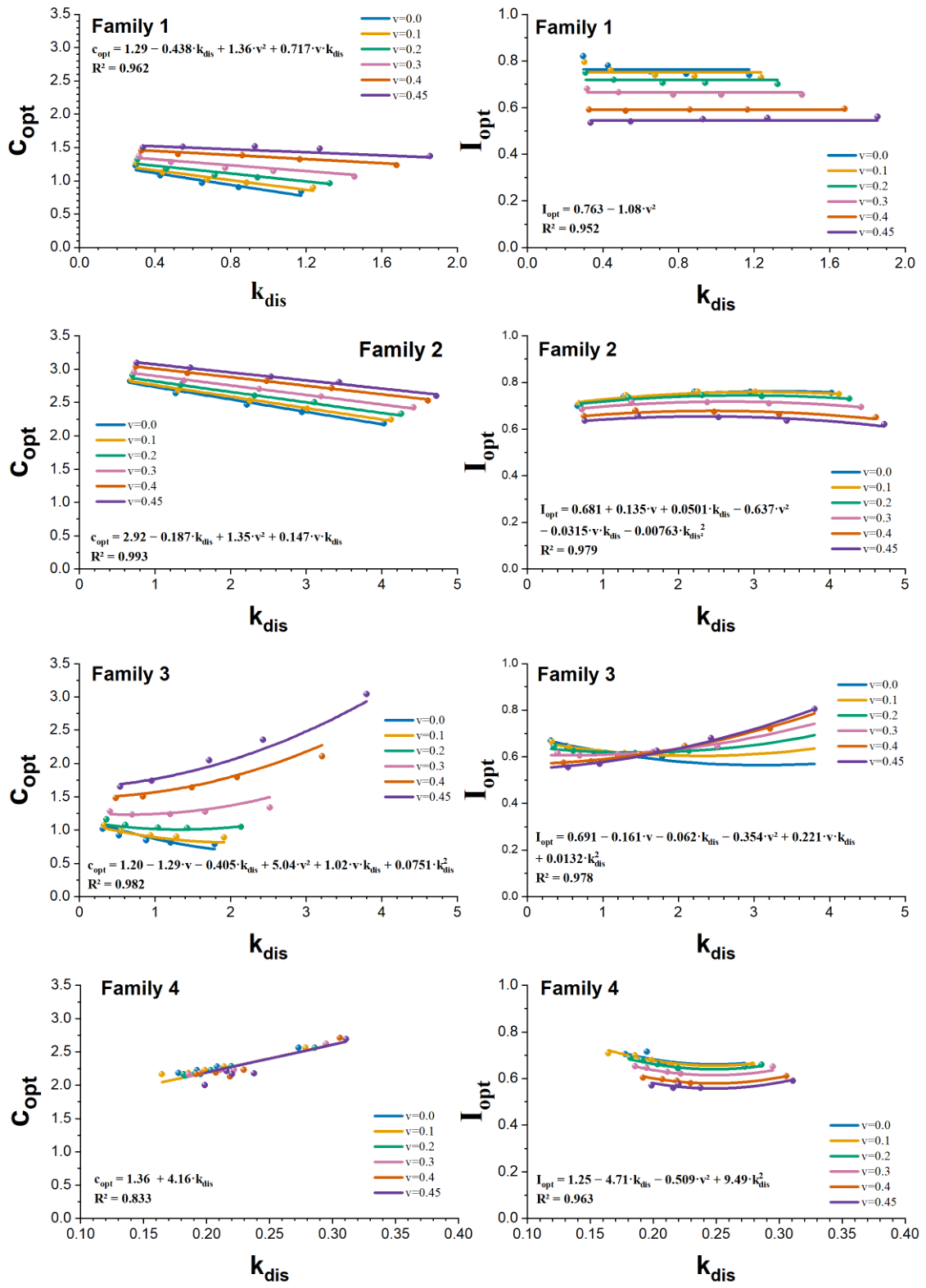
The Pearson correlation between and within the calibration data is modest in every family (–), confirming that the two predictors are only weakly collinear and can be treated as independent regressors in the response surfaces.
The case-by-case optima organize into smooth, low-curvature surfaces over the plane, and the quadratic fits of Table 1, Table 2, Table 3 and Table 4 achieve coefficients of determination ranging from (Profile Family 4, c-surface) to (Profile Family 2, c-surface), with a median of across the eight fitted surfaces. The residual scatter of the surface-predicted parameters about the individual optima translates into only a modest degradation of profile accuracy relative to the per-case optimum: moving from the per-case optimum to the blind, surface-predicted pair, the family-average WAD increases from 1.20% to 2.21% (Profile Family 1), 2.66% to 2.95% (Profile Family 2), 1.69% to 3.27% (Profile Family 3) and 4.36% to 4.66% (Profile Family 4), with a corresponding RMSPE increase from 1.77% to 2.55%, 3.97% to 4.04%, 2.33% to 3.72% and 5.47% to 5.76%, respectively. This confirms that the two predictors and capture the dominant systematic variation of the optimal and that the blind protocol is viable.
A further simplification emerges from the structure of the calibrated surfaces and from the tolerant, valley-shaped error landscapes of Figure 4. For the Poisson’s ratio most representative of compacted earth materials, , a single universal influence coefficient, , was found to serve all four profile families, combined with just two values of the depth ratio selected from the sign of the dispersion-curve slope alone: for normal profiles ( increasing with D) and for reverse profiles ( decreasing with D). Applied to the cases of the database, this two-constant protocol yields family-average profile errors of WAD = 0.78%, 2.6%, 0.95% and 4.2%, and RMSPE = 1.22%, 3.9%, 1.35% and 5.4%, for Profile Families 1–4 respectively—accuracy fully comparable to that of the response-surface protocol, obtained without evaluating any calibration equation. Since is a reasonable default for the majority of soils, the routine application of SIM thus reduces to a single decision: reading the sign of the slope of the measured dispersion curve and selecting the corresponding value of c. It is worth noting that the surface-wave version of SIM admits exactly the same simplification: there, a single universal depth coefficient for normally dispersive profiles at , and for inversely dispersive ones, was likewise found to suffice in practice [5,6]—suggesting that this collapse to a slope-sign-based universal calibration is a robust structural property of the direct inversion scheme rather than a peculiarity of the plate loading problem.
4.2. Occam Results and the Role of the Regularization Parameter
Figure 6 shows a typical case (Profile Family 1, , ) and encapsulates the pathology of the regularized inversion in a single picture. Two systematic observations emerge. First, the data misfit increases monotonically with , as expected: weak regularization allows near-perfect reproduction of the noise-free settlement curves—at the fitted dispersion curve deviates from the measurements by a mere 1.6%, and both fitted curves in Figure 6b are visually indistinguishable from the reference points. Yet this excellent data fit buys nothing for the profile: at the same the profile error is 12%, and the recovered profile in Figure 6c exhibits the spurious, oscillatory overshoots typical of under-regularized inversion. Second, the profile error exhibits a genuine interior minimum at intermediate —here at , where the profile error drops to 7.7% while the data misfit has already grown to 6.5%—typically one to two orders of magnitude above the smallest swept value. This minimum is, however, invisible to the blind selection criterion: because the synthetic data contain no noise, the misfit–roughness trade-off curve possesses no distinct corner, and the maximum-curvature criterion settles on values of far from the profile-optimal one. This behaviour is consistent with the theoretical result of Vogel [17] on the non-convergence of the L-curve criterion in the small-noise limit, and was found to persist when the L-curve criterion was replaced by generalized cross-validation. It follows that even under idealized, noise-free conditions—and, a fortiori, under field conditions—the operating point of Occam’s inversion cannot be reliably identified from the data alone, and the accuracy actually delivered in blind application falls well short of the best accuracy the method could deliver with an oracle choice of .
A further recurrent feature concerns the deepest, half-space layer of the Occam parametrization. The sensitivity of the settlement observations to the modulus of this layer is nearly zero, so its recovered value is controlled almost entirely by the smoothness penalty rather than by the data—a concrete manifestation of the loss of resolution with depth discussed in Section 1.
4.3. Dispersion-Curve Reproduction Versus Profile Recovery
Table 5 summarizes the benchmark over the four profile families, reporting the family-average WAD and RMSPE of the recovered profiles for both methods, together with the family-average of the forward-recomputed dispersion curves.
Three results stand out. First, the calibrated SIM outperforms Occam’s inversion on the profile-recovery task in every family, by factors ranging from roughly 1.6 (Profile Family 4) to 7 (Profile Family 2) on both metrics: family-average WAD of 2.2–4.7% against 7.4–19.1%, and RMSPE of 2.6–5.8% against 9.4–28.3%. The parity plot of Figure 7 shows that this superiority is not merely a property of the averages: essentially every one of the 120 individual cases lies above the 1:1 line, with the margin most dramatic in Profile Family 2 (Occam 12–37% against SIM 2–4%) and narrowest in Profile Family 4, where the mildest slopes bring the two methods closest together. The figure also reveals a robustness asymmetry: the SIM errors are compressed into a narrow horizontal band (roughly 1–4% in Families 1–3), whereas the Occam errors spread over a several-fold vertical range as and m vary—the calibrated direct inversion is not only more accurate but also far less sensitive to the case parameters. Second, the ordering is reversed on the data-reproduction task: as Figure 8 shows, in Families 2–4 virtually all points lie far below the 1:1 line—Occam reproduces the dispersion curves up to an order of magnitude more closely—while Family 1 is the only family in which the two methods straddle the line. The contrast is most striking in Profile Family 2, where Occam attains = 2.29% while returning the worst profile errors of the entire benchmark (WAD 19.1%, RMSPE 28.3%), and SIM reproduces the data an order of magnitude worse (26.2%) while recovering the profile an order of magnitude better (WAD 2.95%). Third, the gap between RMSPE and WAD is systematically wider for Occam than for SIM, indicating—by the diagnostic property of Section 3.3—that the Occam error is concentrated over narrow depth ranges (shallow layers and the unresolved half-space) rather than diffusely distributed.
The joint reading of Figure 7 and Figure 8 is particularly instructive because the same 120 cases populate both plots: passing from the profile metric to the data metric inverts the ranking of the two methods almost case by case. Occam converts its excess flexibility into data fit, absorbing the information of the settlement curve into whichever of the many compatible profiles the smoothness prior happens to select; SIM instead determines the layer moduli directly from successive observations through peeling and therefore cannot freely adjust them merely to chase a lower data misfit. The joint pattern of Table 5 and Figure 7 and Figure 8 is the central empirical finding of this study: goodness of data fit and goodness of profile recovery are nearly decoupled. A method may traverse the data almost exactly and still deliver a substantially wrong profile, because entire families of profiles are compatible with the same settlement curve; conversely, a resolution-matched, data-driven inversion may recover the true profile accurately even where its forward-recomputed data fit is mediocre. This is the non-uniqueness of the inverse problem made quantitative.
Figure 9 makes the spatial anatomy of the Occam failure visible, and its pattern is the same in all four families: the regularized inversion converges well over the depth ranges that contribute most to the measured settlement—the compliant layers, where the strain energy of the test is concentrated—but loses the profile in the stiff layers, whose contribution to the surface settlement is small. In Profile Family 1 the soft shallow zone is captured almost exactly, while the recovered profile drifts away from the reference within the stiff material at depth; in Profile Family 2 the situation is reversed geometrically but identical in mechanism, with the soft deep material well resolved and the stiff surface crust substantially overshot. Because these poorly recovered stiff zones contribute little to the settlements, their misfit costs Occam almost nothing in the dispersion-curve reproduction—which is precisely why the profile can be lost without the data fit betraying it, completing, at the level of individual layers, the decoupling argument of Figure 7 and Figure 8. The data-driven SIM peeling reconstruction does not exhibit this depth selectivity: its error is distributed thinly over the full depth range (per-panel RMSPE of 0.7–6.2%, against 7.5–24.3% for Occam).
4.4. Behaviour Per Profile Family
Profile Family 2 (exponential reverse) is the most adverse configuration for the regularized inversion. A stiff crust overlying softer material concentrates the stress-induced strains at depth, where the observational sensitivity is weakest, while the smoothness penalty resists the steep negative stiffness gradient near the surface; the combination produces the largest profile errors of the benchmark despite the closest data fit. Profile Family 1 (exponential normal) is the most favourable for both methods, the shallow soft material being well sampled by the small diameters. The linear families (Profile Families 3 and 4) occupy intermediate positions. For SIM, the reverse variant (Family 4) remains more challenging than the normal one (Family 3), consistent with the pattern observed for the exponential families; for Occam, by contrast, no consistent ordering holds between the two linear families, with Family 4 in fact showing the smaller profile errors of the pair. For SIM, the compliance-based differencing variant () was systematically selected by the optimization in the normal families (Profile Families 1 and 3), and the modulus-based variant () in the reverse families (Profile Families 2 and 4), consistent with the sign-of-slope selection rule of Section 2.3.
5. Discussion
5.1. Why Regularized Inversion Underperforms Here
The results admit a coherent interpretation in the classical bias–variance framework of statistical estimation. Occam’s inversion equips a flexible, ()-parameter model with a generic smoothness prior on the log-modulus profile, whose strength must be tuned through . SIM takes a different route: peeling converts each successive observation into a layer modulus, while only the modulus-scale coefficient I and the depth-localization coefficient c require calibration. The recovered profile is therefore not a two-parameter function; it contains one data-derived modulus per representative depth interval. This resolution-matched construction avoids introducing freely adjustable layer values whose principal effect may be to improve the fit of the settlement curve. Occam’s inversion, by contrast, must distribute the information of the same M observations over coupled unknowns, leaving the solution sensitive to , to the decreasing depth sensitivity of the kernel and to smoothing bias at steep gradients. The advantage of SIM in this benchmark is therefore not the imposition of a prescribed profile shape, but the direct use of the information added by each plate diameter.
The failure of the blind -selection deserves separate emphasis. The L-curve and related criteria presuppose measurement noise whose progressive suppression generates the characteristic misfit–roughness corner; in its absence, no corner exists and the criteria degenerate [17]. Field data contain noise, and one might expect the criteria to function better there; but field data equally contain correlated model errors (non-elastic behaviour, lateral heterogeneity, plate–soil contact effects) that violate the random-noise assumption in the opposite direction. In either regime, the operating point of the regularized inversion is not reliably identifiable from the data alone, and the accuracy gap between the oracle-best and the blindly selected —clearly visible in Figure 6—should be regarded as an intrinsic cost of the approach in this application.
5.2. Robustness of the Universal SIM Calibration
At the representative value , the SIM calibration reduces to one influence coefficient and two depth ratios. The same applies to all four profile families, while c depends only on the direction of the measured dispersion curve: when increases with plate diameter and when it decreases. These values remain unchanged for the linear and exponential cases and for all five values of m. Despite this simple rule, the family-average errors remain low (WAD = 0.78–4.2% and RMSPE = 1.22–5.4%). This shows that the calibration is controlled mainly by the direction of the measured stiffness trend, not by the exact analytical form or gradient of the reference profile.
This result follows naturally from the peeling procedure. SIM does not fit a linear or exponential function to the unknown . Instead, for plates ordered by increasing diameter, it uses the change between two consecutive apparent-modulus or apparent-compliance values to estimate the modulus of the additional depth interval sampled by the larger plate. Repeating this step produces one modulus for each representative depth interval and therefore a layered, data-derived profile. The coefficient I corrects the modulus scale, whereas c converts plate diameter to representative depth through . The four reference families are used only to calibrate and test these two conversions over a broad range of responses; their shapes are not imposed on the recovered profile. Thus, common values of I and c do not produce a common profile: different measured dispersion curves still generate different layer moduli through peeling. The common calibration simply makes this recovery direct and reproducible, without a starting model, regularization parameter or iterative search.
5.3. Practical Implications
For practice, the results support a simple protocol: perform plate bearing tests at a common contact pressure with at least four plate diameters—the minimum recommended for design and evaluation purposes [2]—spanning as wide a range as logistics permit; construct the nominal apparent-modulus curve; classify the profile family from its shape; evaluate from the calibrated surfaces using the known or estimated Poisson’s ratio; and apply the closed-form inversion. For the most common case in practice, , even the calibration equations become unnecessary: the universal values of Section 4.1 apply, with throughout and the depth ratio chosen solely from the slope of the measured curve— if increases with D, if it decreases. The entire procedure requires no specialized inversion software, no regularization tuning and no starting model, and its accuracy on the benchmark families exceeds that of a properly configured regularized inversion by a wide margin.
6. Conclusions
A systematic synthetic benchmark of 120 cases spanning four stiffness-profile families, six Poisson’s ratios and five profile slopes was used to assess the recovery of depth-dependent soil modulus profiles from multi-diameter plate bearing data. A classical Occam-type smoothness-constrained inversion was compared with SIM, a closed-form, layer-by-layer method governed by two calibration coefficients. The main conclusions are as follows.
- 1.
- SIM recovers the stiffness profile by peeling successive plate observations rather than by fitting a prescribed function to . Each peeling step estimates the modulus associated with the additional depth interval sampled by the next plate diameter. The coefficient I sets the modulus scale and c assigns the recovered values to representative depths through ; they do not define the shape of the recovered profile. Accordingly, the linear and exponential reference profiles used in this study constitute the calibration and validation domain, not shapes imposed by SIM.
- 2.
- Over the complete 120-case benchmark, the calibrated and blindly applied SIM achieved family-average WAD of 2.2–4.7% and RMSPE of 2.6–5.8%. Its errors were lower and less variable than those of Occam’s inversion across all four profile families, demonstrating stable profile recovery over the investigated ranges of m and without a starting model, iterative optimization or a regularization parameter.
- 3.
- At , the calibration reduces to a common rule. The same influence coefficient, , applies to all four profile families and all tested values of m, while c changes only with the sign of the measured –D slope: for an increasing curve and for a decreasing curve. Neither the linear nor the exponential form, nor the magnitude of the profile gradient, is required. This rule yields family-average WAD of 0.78–4.2% and RMSPE of 1.22–5.4%, making SIM directly applicable without evaluating a calibration equation.
- 4.
- For other values of , the optimal I and c vary smoothly with the Poisson’s ratio and the data-derived descriptor . The calibrated response surfaces retain the blind character of SIM: the required coefficients are obtained from the measured dispersion curve and , not from knowledge of the reference profile.
- 5.
- Occam’s inversion reproduced the settlement–diameter curves more closely, yet returned profile errors 1.6–7 times larger than those of SIM. Its largest errors occurred in stiffness zones to which settlement is weakly sensitive, while the automatic L-curve choice of could not identify the profile-optimal solution. The resulting reversal between data fit and profile accuracy demonstrates the practical non-uniqueness of the settlement-based inverse problem and shows why close data reproduction alone is not a sufficient inversion criterion.
- 6.
- These results provide a strong basis for applying SIM to multi-diameter plate tests. Further work should test the common calibration under realistic measurement variability and full-scale field conditions and extend the calibration domain to sharply layered and multi-transition stiffness arrangements.
Author Contributions
Conceptualization, methodology, and writing—original draft preparation, P.P.; formal analysis, G.O.; writing—review and editing, N.D. All authors have read and agreed to the published version of the manuscript.
Funding
This research received no external funding.
Institutional Review Board Statement
Not applicable.
Informed Consent Statement
Not applicable.
Data Availability Statement
The interactive computational tool implementing the forward model, both inversion methods and the statistical calibration, together with the complete synthetic database, is available from the authors upon reasonable request.
Conflicts of Interest
The authors declare no conflicts of interest.
Abbreviations
The following abbreviations are used in this manuscript:
| FWD | Falling-Weight Deflectometer |
| GCV | Generalized Cross-Validation |
| NDT | Non-Destructive Testing |
| RMSPE | Root-Mean-Square Percentage Error |
| SIM | Simplified Inversion Method |
| WAD | Weighted Absolute Deviation |
References
- DIN 18134:2012-04; Soil—Testing Procedures and Testing Equipment—Plate Load Test. Deutsches Institut für Normung: Berlin, Germany, 2012.
- ASTM D1195/D1195M-21; Standard Test Method for Repetitive Static Plate Tests of Soils and Flexible Pavement Components for Use in Evaluation and Design of Airport and Highway Pavements. ASTM International: West Conshohocken, PA, USA, 2021.
- Mayne, P.W.; Poulos, H.G. Approximate displacement influence factors for elastic shallow foundations. J. Geotech. Geoenviron. Eng. 1999, 125, 453–460. [Google Scholar] [CrossRef]
- Hallo, M.; Imperatori, W.; Panzera, F.; Fäh, D. Joint multizonal transdimensional Bayesian inversion of surface wave dispersion and ellipticity curves for local near-surface imaging. Geophys. J. Int. 2021, 226, 627–659. [Google Scholar] [CrossRef]
- Pelekis, P.C.; Athanasopoulos, G.A. An overview of surface wave methods and a reliability study of a new simplified inversion technique. Soil Dyn. Earthq. Eng. 2011, 31, 1654–1668. [Google Scholar] [CrossRef]
- Pelekis, P.C.; Athanasopoulos, G.A. Application of a simplified inversion technique to published surface wave dispersion data—Comparisons with advanced methods of inversion. In GeoCongress 2012: State of the Art and Practice in Geotechnical Engineering; ASCE: Reston, VA, USA, 2012; pp. 2716–2725. [Google Scholar]
- Rada, G.R.; Nazarian, S.; Visintine, B.A.; Siddharthan, R.V.; Thyagarajan, S. Pavement Structural Evaluation at the Network Level; Publication No. FHWA-HRT-15-074; U.S. Department of Transportation: Washington, DC, USA, 2016. [Google Scholar]
- Sharma, S.; Das, A. Backcalculation of pavement layer moduli from falling weight deflectometer data using an artificial neural network. Can. J. Civ. Eng. 2008, 35, 57–66. [Google Scholar] [CrossRef]
- Constable, S.C.; Parker, R.L.; Constable, C.G. Occam’s inversion: A practical algorithm for generating smooth models from electromagnetic sounding data. Geophysics 1987, 52, 289–300. [Google Scholar] [CrossRef]
- DeGroot-Hedlin, C.; Constable, S. Occam’s inversion to generate smooth, two-dimensional models from magnetotelluric data. Geophysics 1990, 55, 1613–1624. [Google Scholar] [CrossRef]
- Tikhonov, A.N.; Arsenin, V.Y. Solutions of Ill-Posed Problems; Winston & Sons: Washington, DC, USA, 1977. [Google Scholar]
- Portniaguine, O.; Zhdanov, M.S. Focusing geophysical inversion images. Geophysics 1999, 64, 874–887. [Google Scholar] [CrossRef]
- Vargas Huitzil, E.; Morzfeld, M.; Constable, S. RamBO: Randomized blocky Occam, a practical algorithm for generating blocky models and associated uncertainties. Geophys. J. Int. 2025, 241, 567–579. [Google Scholar] [CrossRef]
- Hansen, P.C.; O’Leary, D.P. The use of the L-curve in the regularization of discrete ill-posed problems. SIAM J. Sci. Comput. 1993, 14, 1487–1503. [Google Scholar] [CrossRef]
- Farquharson, C.G.; Oldenburg, D.W. A comparison of automatic techniques for estimating the regularization parameter in non-linear inverse problems. Geophys. J. Int. 2004, 156, 411–425. [Google Scholar] [CrossRef]
- Zainalpour, A.; Kamali, G.; Moradzadeh, A. Optimal selection of regularization parameter in magnetotelluric data inversion. Acta Geod. Geophys. 2022, 57, 245–263. [Google Scholar] [CrossRef]
- Vogel, C.R. Non-convergence of the L-curve regularization parameter selection method. Inverse Probl. 1996, 12, 535–547. [Google Scholar] [CrossRef]
- Malinverno, A. Parsimonious Bayesian Markov chain Monte Carlo inversion in a nonlinear geophysical problem. Geophys. J. Int. 2002, 151, 675–688. [Google Scholar] [CrossRef]
- Shaw, R.; Srivastava, S. Particle swarm optimization: A new tool to invert geophysical data. Geophysics 2007, 72, F75–F83. [Google Scholar] [CrossRef]
- Gibson, R.E. Some results concerning displacements and stresses in a non-homogeneous elastic half-space. Géotechnique 1967, 17, 58–67. [Google Scholar] [CrossRef]
- Brown, P.T.; Gibson, R.E. Surface settlement of a deep elastic stratum whose modulus increases linearly with depth. Can. Geotech. J. 1972, 9, 467–476. [Google Scholar] [CrossRef]
- Selvadurai, A.P.S. The settlement of a rigid circular foundation resting on a half-space exhibiting a near surface elastic non-homogeneity. Int. J. Numer. Anal. Methods Geomech. 1996, 20, 351–364. [Google Scholar] [CrossRef]
- Ahn, J.; Cote, J.; Robinson, B.; Gabr, M.A.; Borden, R.H. Inverse analysis of plate load tests to assess subgrade resilient modulus. Transp. Res. Rec. J. Transp. Res. Board 2009, 2101, 109–117. [Google Scholar] [CrossRef]
Figure 3.
Dispersion curves, S–D and –D, for each profile family, for all combinations of m and (30 curves per panel; , nominal ). The functional form fitted to the nominal apparent-modulus curve to extract (Section 3.5) is annotated on each –D panel, together with the approximate range of spanned by the family’s grid.
Figure 3.
Dispersion curves, S–D and –D, for each profile family, for all combinations of m and (30 curves per panel; , nominal ). The functional form fitted to the nominal apparent-modulus curve to extract (Section 3.5) is annotated on each –D panel, together with the approximate range of spanned by the family’s grid.
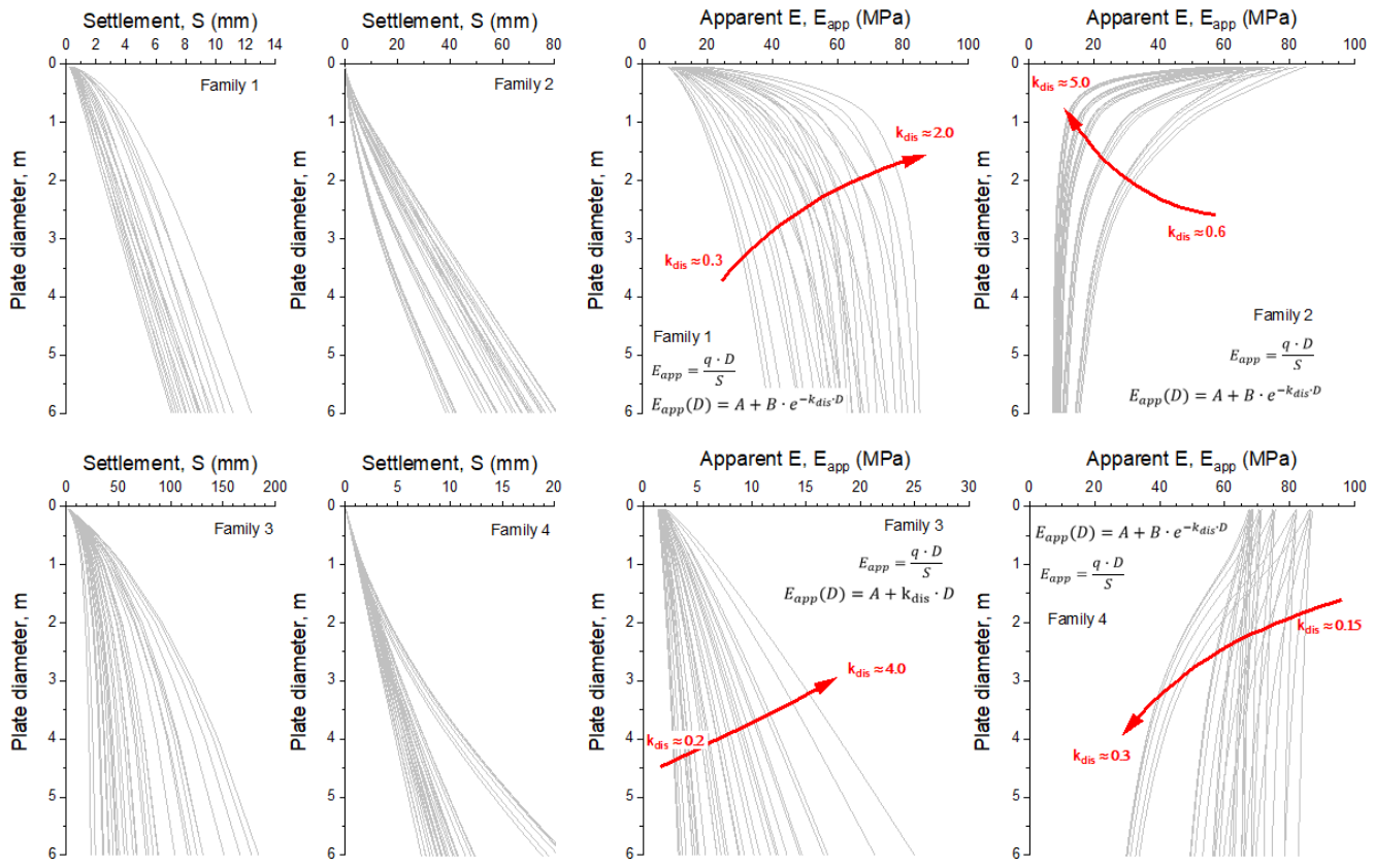
Figure 4.
Error landscapes of the SIM inversion in the parameter plane for a representative case of each profile family (, ): left column, WAD; right column, RMSPE; rows, Profile Families 1–4 (top to bottom). The cross marks the optimum identified by the grid search. Colour scale saturated at 10%.
Figure 4.
Error landscapes of the SIM inversion in the parameter plane for a representative case of each profile family (, ): left column, WAD; right column, RMSPE; rows, Profile Families 1–4 (top to bottom). The cross marks the optimum identified by the grid search. Colour scale saturated at 10%.
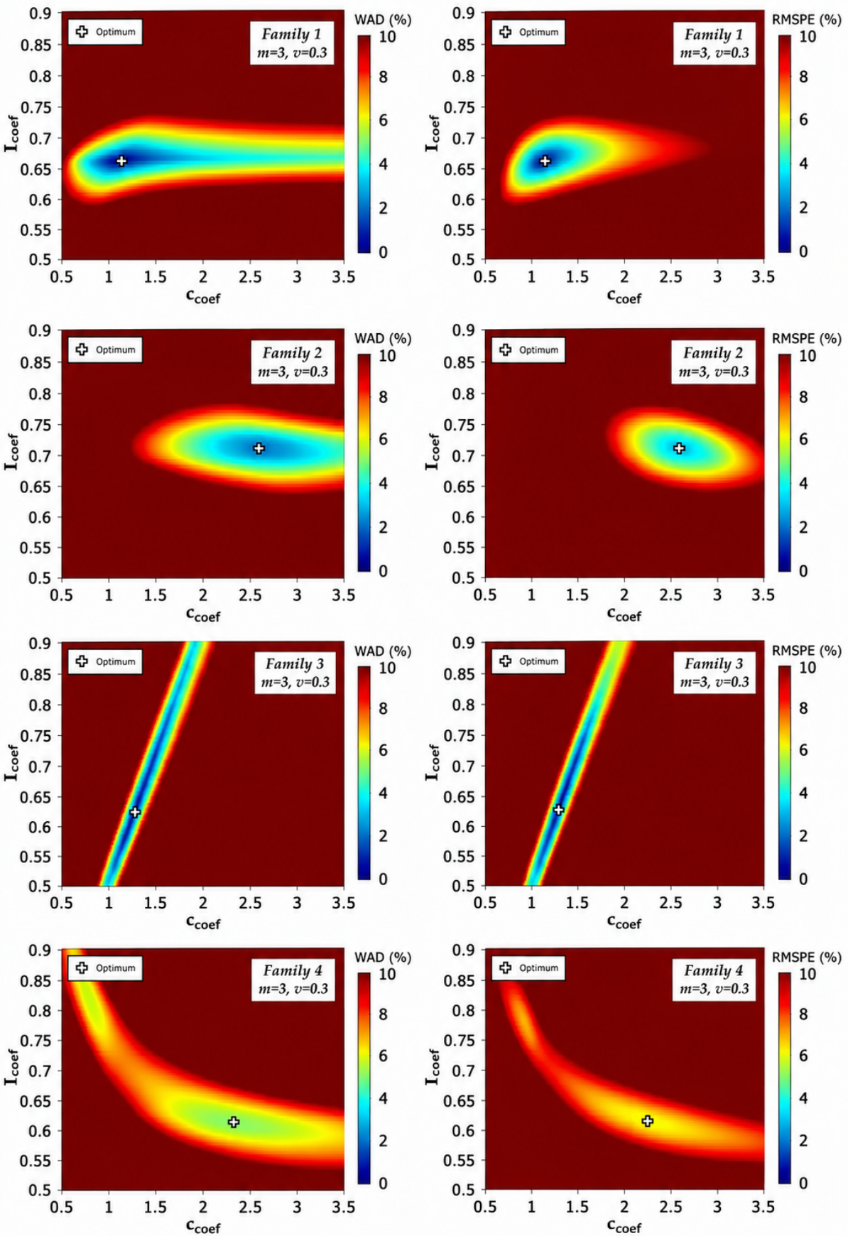
Figure 6.
Typical Occam inversion (Profile Family 1, , ): (a) profile error (RMSPE against the reference profile, left axis) and data misfit ( of the fitted dispersion curve, right axis) as functions of the regularization parameter , with two values marked—, on the small- plateau, and , the profile-optimal value; (b) reference and fitted settlement–diameter curves for the two marked values of ; (c) reference stiffness profile and the profiles recovered at the two marked values of .
Figure 6.
Typical Occam inversion (Profile Family 1, , ): (a) profile error (RMSPE against the reference profile, left axis) and data misfit ( of the fitted dispersion curve, right axis) as functions of the regularization parameter , with two values marked—, on the small- plateau, and , the profile-optimal value; (b) reference and fitted settlement–diameter curves for the two marked values of ; (c) reference stiffness profile and the profiles recovered at the two marked values of .
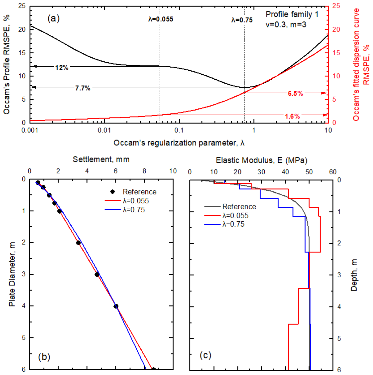
Figure 7.
Case-by-case (parity) comparison of the profile errors (RMSPE) of Occam’s inversion (vertical axis) and the blindly applied SIM (horizontal axis) for the four profile families; marker colour denotes the Poisson’s ratio and marker shape the profile parameter m. Points above the dashed 1:1 line correspond to cases in which SIM recovers the stiffness profile more accurately.
Figure 7.
Case-by-case (parity) comparison of the profile errors (RMSPE) of Occam’s inversion (vertical axis) and the blindly applied SIM (horizontal axis) for the four profile families; marker colour denotes the Poisson’s ratio and marker shape the profile parameter m. Points above the dashed 1:1 line correspond to cases in which SIM recovers the stiffness profile more accurately.
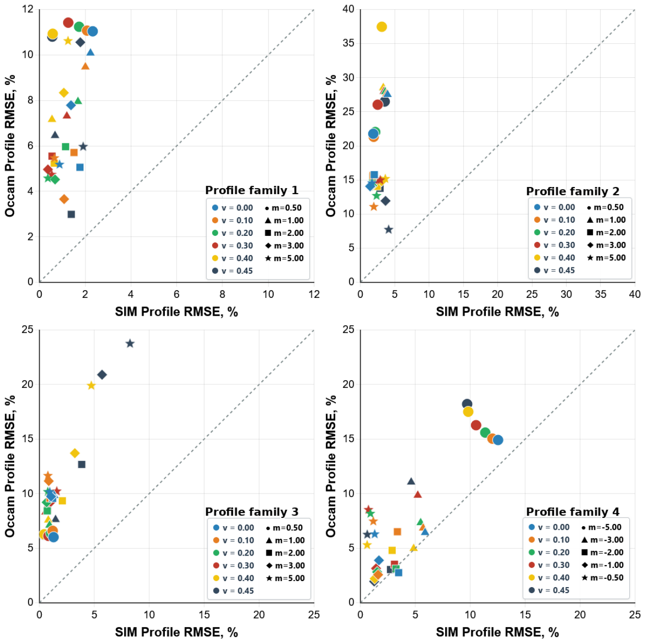
Figure 8.
Case-by-case (parity) comparison of the dispersion-curve reproduction errors () of Occam’s inversion (vertical axis) and SIM (horizontal axis) for the four profile families; symbols as in Figure 7. Points below the dashed 1:1 line correspond to cases in which Occam reproduces the measured dispersion curve more closely.
Figure 8.
Case-by-case (parity) comparison of the dispersion-curve reproduction errors () of Occam’s inversion (vertical axis) and SIM (horizontal axis) for the four profile families; symbols as in Figure 7. Points below the dashed 1:1 line correspond to cases in which Occam reproduces the measured dispersion curve more closely.
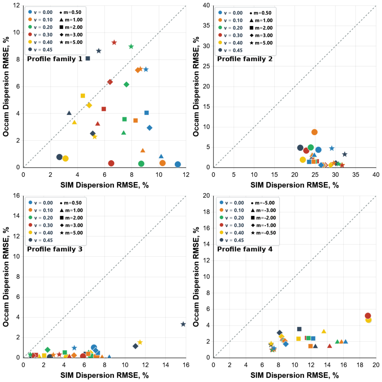
Figure 9.
Representative recovered profiles for one case of each profile family (, ): reference profile, blindly applied SIM, and Occam’s inversion at the automatically selected . The RMSPE of each recovered profile is given in the legends.
Figure 9.
Representative recovered profiles for one case of each profile family (, ): reference profile, blindly applied SIM, and Occam’s inversion at the automatically selected . The RMSPE of each recovered profile is given in the legends.
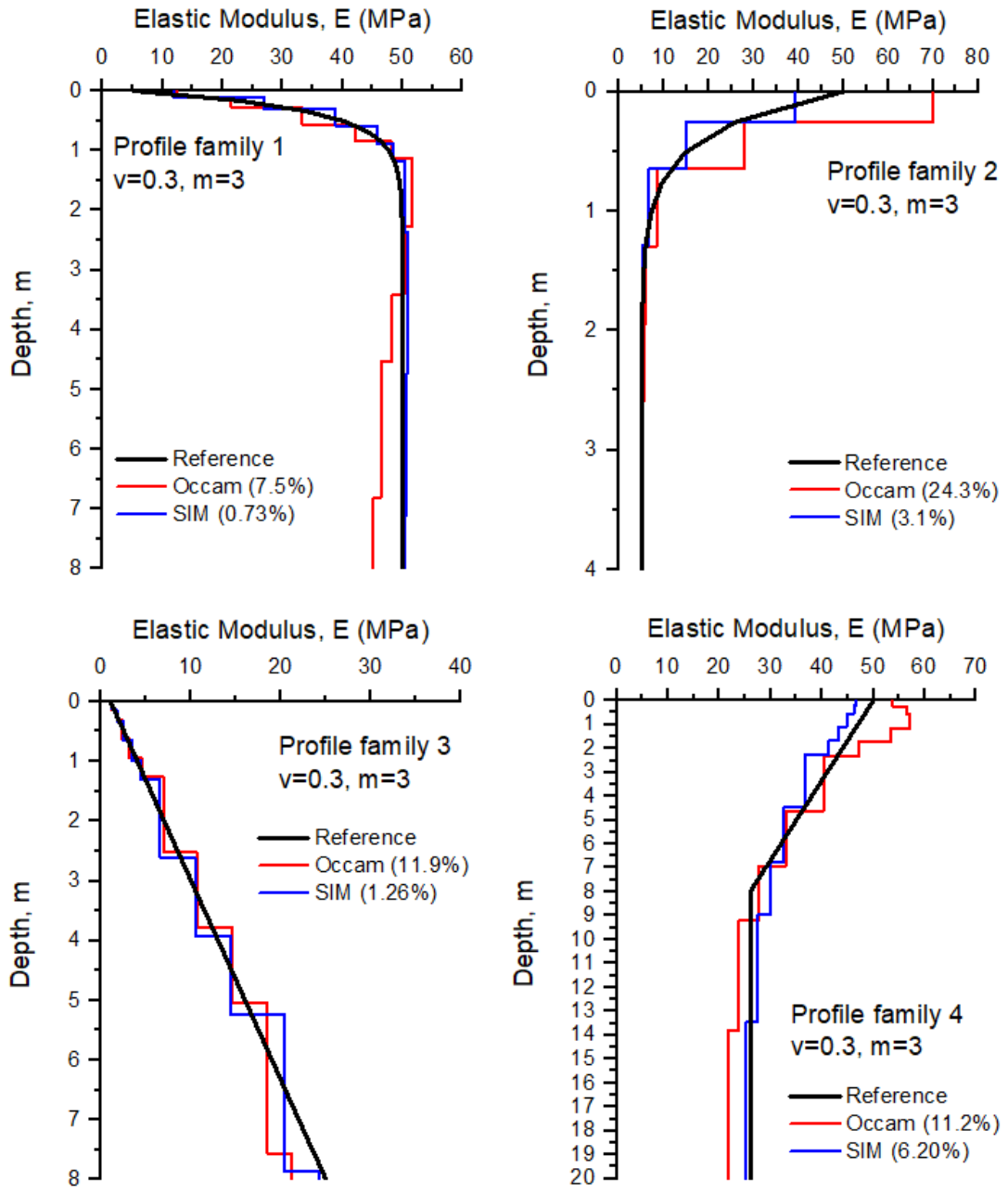

Table 1.
RMSPE-optimized response-surface coefficients for Profile Family 1 (exponential normal).
| Term | ||
|---|---|---|
| Intercept | 0.7627 (0.00518)*** | 1.291 (0.0256)*** |
| — | — | |
| — | −0.4376 (0.0394)*** | |
| −1.075 (0.0459)*** | 1.361 (0.212)*** | |
| — | 0.7165 (0.115)*** | |
| — | — | |
| 0.9515 | 0.9623 | |
| n (dof) | 30 (28) | 30 (26) |
Table 2.
RMSPE-optimized response-surface coefficients for Profile Family 2 (exponential reverse).
| Term | ||
|---|---|---|
| Intercept | 0.6806 (0.00616)*** | 2.921 (0.0122)*** |
| 0.1351 (0.0327)*** | — | |
| 0.05007 (0.00453)*** | −0.1871 (0.00570)*** | |
| −0.6371 (0.0635)*** | 1.346 (0.104)*** | |
| −0.03151 (0.00638)*** | 0.1473 (0.0183)*** | |
| −0.007627 (0.000890)*** | — | |
| 0.9794 | 0.9926 | |
| n (dof) | 30 (24) | 30 (26) |
Table 3.
RMSPE-optimized response-surface coefficients for Profile Family 3 (linear normal).
| Term | ||
|---|---|---|
| Intercept | 0.6912 (0.00519)*** | 1.199 (0.0521)*** |
| −0.1612 (0.0352)*** | −1.293 (0.354)** | |
| −0.06196 (0.00556)*** | −0.4052 (0.0559)*** | |
| −0.3538 (0.0728)*** | 5.038 (0.731)*** | |
| 0.2213 (0.0169)*** | 1.024 (0.170)*** | |
| 0.01319 (0.00210)*** | 0.07509 (0.0211)** | |
| 0.9784 | 0.9822 | |
| n (dof) | 30 (24) | 30 (24) |
Table 4.
RMSPE-optimized response-surface coefficients for Profile Family 4 (linear reverse).
| Term | ||
|---|---|---|
| Intercept | 1.245 (0.0686)*** | 1.360 (0.0788)*** |
| — | — | |
| −4.710 (0.587)*** | 4.161 (0.352)*** | |
| −0.5086 (0.0241)*** | — | |
| — | — | |
| 9.488 (1.21)*** | — | |
| 0.9632 | 0.8330 | |
| n (dof) | 30 (26) | 30 (28) |
Table 5.
Family-averaged profile errors (WAD, RMSPE against the reference profile) and dispersion-curve reproduction errors () for Occam’s inversion (automatic ) and the calibrated, blindly applied SIM. Profile family numbering as in Section 3.1.
Table 5.
Family-averaged profile errors (WAD, RMSPE against the reference profile) and dispersion-curve reproduction errors () for Occam’s inversion (automatic ) and the calibrated, blindly applied SIM. Profile family numbering as in Section 3.1.
| Family | Occam | SIM | Dispersion (%) | |||
|---|---|---|---|---|---|---|
| WAD (%) | RMSPE (%) | WAD (%) | RMSPE (%) | Occam | SIM | |
| 1 (exp. normal) | 7.39 | 9.40 | 2.21 | 2.55 | 4.01 | 6.88 |
| 2 (exp. reverse) | 19.10 | 28.28 | 2.95 | 4.04 | 2.29 | 26.23 |
| 3 (lin. normal) | 10.19 | 12.74 | 3.27 | 3.72 | 0.51 | 5.42 |
| 4 (lin. reverse) | 7.54 | 9.43 | 4.66 | 5.76 | 2.53 | 12.62 |
Disclaimer/Publisher’s Note: The statements, opinions and data contained in all publications are solely those of the individual author(s) and contributor(s) and not of MDPI and/or the editor(s). MDPI and/or the editor(s) disclaim responsibility for any injury to people or property resulting from any ideas, methods, instructions or products referred to in the content. |
© 2026 by the authors. Licensee MDPI, Basel, Switzerland. This article is an open access article distributed under the terms and conditions of the Creative Commons Attribution (CC BY) license (http://creativecommons.org/licenses/by/4.0/).
Copyright: This open access article is published under a Creative Commons CC BY 4.0 license, which permit the free download, distribution, and reuse, provided that the author and preprint are cited in any reuse.


