

Submitted:
06 August 2026
Posted:
07 August 2026
You are already at the latest version
Abstract
Accurate prediction of residual flexural strengths is essential for the structural design and performance assessment of steel fibre reinforced concrete (SFRC). While machine learning models have recently demonstrated strong predictive capability, most of the existing approaches rely on heuristic feature selection, unconstrained architectures, and random validation splits that may overestimate generalization capacity. This study proposes a Hard-constrained Mechanics-Informed Neural Network framework for predicting SFRC residual strengths across independent experimental studies. A multi-study database comprising 860 observations from 18 experimental assemblies was analysed to identify statistically dominant and physically interpretable predictors. Based on exploratory statistical analysis and micromechanical assessment, a hierarchical shared-backbone neural network architecture was developed. Physical admissibility was enforced structurally through non-negativity constraints, monotonic dependence on effective fibre bridging capacity, and bounded signed transitions between CMOD stages. Model performance was evaluated using five-fold group-based cross-validation, where entire studies were excluded from training to rigorously assess generalization. The proposed architecture achieved predictive performance comparable to or exceeding conventional neural networks and ensemble models, while eliminating physically inadmissible predictions and reducing fold-to-fold variability. The results demonstrate that embedding mechanical principles directly into neural network architecture enhances robustness and interpretability without compromising accuracy. The proposed hard-constrained Physics-Informed Neural Networks (PINN) framework provides a transferable methodology for physics-guided machine learning in structural materials modelling.
Keywords:
steel fibre reinforced concrete
; residual flexural strength
; physics-informed neural network
; hard architectural constraints
; group-based cross-validation
; reinforcement index
1. Introduction
The use of Steel Fibre Reinforced Concrete (SFRC) in structural engineering has increased, mainly due to its ability to control cracks and provide post-cracking capacity. Based on research by Romualdi and Batson (1963) [1], its performance depends on discrete fibres arresting crack growth. This process was further defined through studies on fibre pull-out [2] and fracture mechanics [3]. Recent work focuses on sustainability; evidence suggests recycled steel fibres offer tensile benefits similar to commercial fibres but with lower embodied carbon [4]. For instance, ultra-high-performance concrete (UHPC) achieves its ductile behaviour and strain-hardening properties through the inclusion of steel fibres, which provide distributed bridging across the matrix [5,6].
Building upon these micromechanical foundations, the practical application of SFRC deviates from conventional reinforced concrete. Whereas tensile resistance is typically localised in discrete bars, SFRC provides distributed crack-bridging through randomly oriented fibres [7]. This mechanism is beneficial for industrial slabs, tunnel linings, and earthquake-resistant components, where serviceability and ultimate limit states are dictated by post-cracking performance.
To characterise this response, the present study defines the flexural behaviour of SFRC through residual strengths (fR1, fR2, fR3 and fR4), determined at specific crack mouth opening displacement (CMOD) intervals. These parameters, measured in accordance with EN 14651 [8], constitute the foundational data structure for the proposed Physics-Informed Neural Network (PINN) model. Although the model's architecture is intrinsically coupled with this specific testing protocol, the framework establishes a versatile methodological basis. Consequently, the approach may be adapted to alternative standards, such as ASTM C1609 [9], thereby supporting the broader development of future PINN models based on varied experimental definitions of flexural performance.
Contemporary frameworks, such as the fib Model Code 2010 [10] and ACI 318-19 [11], incorporate residual strength-based formulations that enable the partial or full replacement of conventional reinforcement [12]. As these standards are progressively adopted globally—including the Spanish Structural Code [13] and Eurocode 2 [14]—the accurate prediction of residual strengths becomes essential for safe structural applications. Given the non-linear complexity of these parameters, identifying reliable predictive patterns is paramount for efficient structural design.
Unlike traditional concrete, where tensile resistance is localised in bars, SFRC provides distributed bridging through randomly oriented fibres. This mechanism is beneficial for industrial slabs, tunnel linings, and seismic components, where post-cracking behaviour governs serviceability and limit states. The flexural performance of SFRC is defined by residual strengths (fR1, fR2, fR3, and fR4), measured at specific CMOD levels according to EN 14651 (2007) [8]. These parameters quantify the capacity of cracked sections and form the basis for structural design. Contemporary frameworks, such as the fib Model Code 2010, use these formulations to determine the structural contribution of fibres, allowing for the partial or full replacement of conventional reinforcement. This approach is now integrated into international standards, including EN 1992-1-1 (2004) [15], ACI 318-19 (2019) (ACI Committee 318, 2019- ASTM C-1609), and various European guidelines [13]. Consequently, predicting residual strengths accurately is fundamental for code-based application of SFRC.
Predicting residual strengths is challenging due to the multiscale mechanisms involved. Post-cracking behaviour is controlled by microscale fibre–matrix interactions, such as debonding and frictional pull-out, alongside mesoscale variability in fibre orientation (Figure 1). These emergent responses depend on matrix strength, fibre tensile strength, and geometric efficiency—specifically aspect ratio and volume fraction. Recent evidence from 887 tests [7] confirms that fibre parameters dominate advanced crack stages while matrix strength influences the limit of proportionality. Traditional empirical models, such as regression-based formulations, often lack robustness and transferability across different fibre geometries or matrix types. For example, models calibrated for straight fibres frequently fail for hooked-end steel fibres. These limitations highlight the inadequacy of purely empirical approaches in capturing non-linear complexities. Consequently, there is a clear need for robust data-driven frameworks that can internalise these dependencies across diverse datasets.
Machine learning (ML) techniques—including neural networks and ensemble methods—have shown significant promise in overcoming the limitations of empirical models by accurately predicting the compressive and flexural properties of cementitious materials [4,16,17,18,19]. In the context of SFRC, these architectures have been successfully deployed to estimate shear capacity and residual strengths [20,21]. However, two critical methodological issues persist in the current literature. First, a reliance on random train–test splits often causes data leakage by mixing samples from the same experimental campaigns across datasets. This practice artificially inflates performance metrics and masks a model's inability to generalise to independent experimental datasets [22,23]. Second, most ML models employ unconstrained architectures that prioritise error minimisation over physical validity. Such models frequently produce physically inadmissible results, such as negative strengths or non-monotonic trends. Furthermore, treating f1-f4 as independent outputs ignores their inherent sequential dependence, where each crack opening stage inherits the mechanical state of the preceding level.
To address these limitations, this study adopts Physics-Informed Neural Networks (PINNs), a framework that incorporates physical principles directly into the learning process [24,25,26]. While PINNs typically embed differential equations, this work extends the framework to inequality-constrained structural modelling. In SFRC, physically consistent behaviour dictates that residual strengths must be non-negative, exhibit monotonic dependence on fibre bridging capacity, and evolve sequentially as crack openings increase. Embedding these constraints transforms the problem into admissible function approximation, restricting the hypothesis space to physically meaningful solutions.
Consequently, hard-constrained PINN framework is used in this study for predicting residual strengths (f1-f4), integrating micromechanical reasoning with architectural constraint enforcement and a group-based validation protocol (GroupKFold by Study) to rigorously assess cross-study generalisation.
The key contributions of this work are:
- i.
- Statistical dominance analysis: A multi-study database analysis—using Pearson correlation and VIF-based diagnostics—confirms the dominance of the reinforcement index (RI) and justifies the feature engineering decisions.
- i.
- ii. Physics-driven architecture: The network input space and architecture are derived from micromechanical reasoning, incorporating interaction terms that reflect fibre-matrix physics.
- i.
- iii. Architectural constraint enforcement: Physical constraints are enforced to guarantee non-negativity, monotonicity, and bounded sequential evolution, ensuring mechanical coherence across all predictions.
- i.
- iv. Study-level cross-validation: A rigorous group-based partitioning framework aligns model evaluation with real-world generalisation requirements.
The central research question addressed is: Can a hard-constrained, physics-informed neural architecture—whose hypothesis space is governed by inequality-based mechanical principles—achieve reliable cross-study generalisation in predicting the residual flexural strengths fR1-fR4 of steel fibre reinforced concrete? By addressing this question, this work aims to advance data-driven modelling from purely empirical prediction towards mechanically admissible and transferable predictive models.
2. Method
2.1. Experimental and Synthetic Database
2.1.1. Experimental Database
The experimental database was compiled from published literature and comprises 235 SFRC beam tests reported across 15 independent research datasets [27]. All specimens were tested under the three-point bending test (3PBT) prescribed by EN 14651 [28], providing the residual flexural tensile strengths at CMOD of 0.5, 1.5, 2.5, and 3.5 mm, respectively.
Each observation includes six input variables with RI = , and four target outputs Missing outputs are present in a subset of the data: 21 entries lack while 72 entries lack Rather than introducing imputation bias in the response variables, incomplete observations were retained and handled through a masked loss formulation (Section 3.6), ensuring that only available targets contribute to the optimization process.
The dataset was expanded to 860 samples through controlled resampling to improve numerical stability during training. This procedure does not introduce new information but modifies the effective empirical risk by reweighting observations. Such implicit weighting is essential in heterogeneous multi-study datasets, where uneven coverage of the input space and study-level imbalances can bias the learning process. Resampling was therefore used to enhance the representation of high-sensitivity regions—particularly those governed by variations in fibre geometry and reinforcement index—while preserving the original data distribution. Data leakage was prevented by adopting a study-level validation protocol (GroupKFold), ensuring strict separation between training and testing domains.
2.1.2. Synthetic Data Generation
To improve coverage of sparse regions of the experimental domain, an extended set of synthetic samples was generated from the consolidated database by structured interpolation within the range of physically observed input variables where
The synthetic targets were not treated as free numerical outputs; instead, they were required to remain compatible with the same mechanical admissibility conditions later imposed by the HardPINN architecture, namely bounded stage-wise increments and non-decreasing contribution of the bridging index RI. In this sense, the synthetic dataset was constructed as a regularization of the experimentally supported response manifold, intended to densify the learning space without introducing mechanically implausible patterns or extrapolated behaviours outside the observed domain.
2.2. Exploratory Data Analysis
Prior to model development, a systematic exploratory data analysis (EDA) was conducted to characterise the distribution of input features and target variables, identify imbalances in study-level contributions, and motivate feature engineering decisions. Descriptive statistics (count, mean, standard deviation, and quartiles) were computed for all six numeric inputs and the four residual strength targets.
Distribution histograms revealed that the composite bridging capacity is given by the reinforcement index and the fibre tensile strength exhibit pronounced right skewness, with heavy positive tails that would otherwise inflate the effective range of these predictors and impair gradient-based optimisation. The samples-per-study distribution confirmed a significant imbalance in database contributions across the 14 experimental datasets, motivating the adoption of a group-based cross-validation strategy (Section 3.7) to prevent data leakage between training and test folds. A Pearson correlation matrix was computed to quantify linear associations among input features and between inputs and targets, providing guidance for interaction term selection during feature engineering.
2.3. Feature Engineering
2.3.1. Variance-Stabilising Transforms
Three variance-stabilizing transformations were applied to compress heavy-tailed distributions and improve numerical conditioning during training:
- natural logarithm of the reinforcement index after a unit shift to handle zero values, suppressing the positive tail of the RI distribution.
- : natural logarithm of fibre tensile strength, stabilising the right-skewed distribution of fu.
- : square root of compressive strength, a transformation commonly used in concrete mechanics to linearise strength and stiffness relationships.
2.3.2. Physically Motivated Interaction Terms
Four interaction features were constructed to capture synergistic effects between pairs of physical variables that cannot be represented independently:
- : combining of bridging capacity and fibre tensile strength, representing the combined contribution of fibre geometry and material resistance to post-cracking performance.
- : combining of bridging capacity and matrix compressive strength, capturing the interaction between fibre content and matrix quality.
- : combining of fibre length and tensile strength, encoding the total force that a fibre of given length can transmit across a crack.
- : combining of compressive strength and the fibre hooks count indicator, accounting for the combined influence of matrix strength and fibre distribution on residual response.
2.3.3. Final Numeric Feature Set
The complete set of 12 numeric features supplied to the preprocessing pipeline was: , N, , , , , log_fu, sqrt_fc, RI.fu, RI.fc, lf.fu, and fc.N. Additionally, the categorical variable Type (concrete mix category) was encoded separately.
2.4. Preprocessing Pipeline
A scikit-learn ColumnTransformer was used to apply separate preprocessing pipelines to the numeric and categorical feature subsets, ensuring that transformations were fit exclusively on training data within each cross-validation fold to prevent information leakage. The numeric pipeline applied median imputation (SimpleImputer with strategy='median') to handle missing values in the input features, followed by standardization to zero mean and unit variance (StandardScaler). Median imputation was selected over mean imputation due to its robustness to the outliers present in the SFRC database. The categorical pipeline applied most-frequent imputation followed by one-hot encoding (OneHotEncoder with handle_unknown='ignore') of the concrete Type variable, producing binary indicator columns for each of the Six concrete mix categories are represented in the database: conventional concrete (CC), high-strength concrete (HSC, fc ≥ 50 MPa), self-compacting concrete (SCC), high-strength self-compacting concrete (HS-SCC), a hybrid HSC/SCC designation (HSC-SCC), and high-performance steel fiber concrete (HPSFC, fc > 60 MPa with high fiber dosage).The bridging capacity variable given by the reinforcement index was tracked by index (RI_IDX) within the numeric feature array after preprocessing. This index was used in the custom split_X_and_RI function to route the scaled reinforcement index (RI column) through a dedicated monotone pathway in the PINN architecture, separate from all other features.
2.5. Physics-Informed Neural Network Architecture
The HardPINN architecture was implemented in TensorFlow (v2.20.0) using the Keras functional API (tf.keras V3.12.1), enabling the incorporation of custom constraint-enforcing layers (e.g., non-negative weights, bounded transitions) within a differentiable computational graph.
The term 'hard-constrained' refers to the fact that the physical constraints are enforced by the network architecture itself—through layer design and activation function selection—rather than through soft penalty terms added to the loss function. This guarantees constraint satisfaction for every input, including out-of-distribution samples, without requiring tuning of penalty hyperparameters.
2.5.1. Dual-Input Structure
After preprocessing, the input array was split into two streams via the split_X_and_RI function: (i) X_other, containing all standardized features except RI, and (ii) RI_scaled, the standardised reinforcement index. This dual-input design allows RI to be routed through a dedicated non-negative weight pathway, enforcing the physical constraint that residual flexural strength is a monotonically non-decreasing function of the RI.
2.5.2. Shared Feature Representation
The X_other stream was processed through a sequence of fully connected hidden layers with batch normalization and dropout regularisation, producing a shared latent representation from which all four residual strength outputs were subsequently derived. This shared backbone promotes feature reuse across the four CMOD stages and reduces the total number of trainable parameters relative to training four independent models.
2.5.3. Non-Negative Dense Layer (NonNegDense) — Monotonicity Constraint
A custom Keras layer, NonNegDense, was developed to enforce the monotonicity constraint In a standard dense layer, weights W are unconstrained real numbers, allowing the network to learn negative weights that would imply an inverse relationship between RI and fRi—a physically inadmissible outcome. NonNegDense addresses this by parameterizing the weights as:
W = softplus(W_raw) where softplus(x) = log(1 + eˣ) > 0 for all x∈ ℝ
The raw weights are the actual trainable parameters, initialized with Glorot uniform initialization. At inference time, softplus is applied to before the matrix multiplication, guaranteeing that all effective weights are strictly positive. Consequently, an increase in RI always produces a non-negative contribution to each fRi output, regardless of what values converge to during training. The layer also includes an unconstrained bias term b.
2.5.4. BetaTanh Layer — Bounded Signed Increments
The four residual strength values fR1 through fR4 were generated in a sequential, hierarchical manner. The first output, fR1, was produced by a dedicated sub-network and passed through a softplus activation to enforce strict non-negativity. The subsequent outputs fR2, fR3, and fR4 were each computed as a signed increment Δ added to the preceding stage:
Each increment Δi was computed by a custom BetaTanh layer, which bounds the increment within the interval (−β, +β) while allowing gradients to flow freely during backpropagation:
where z is the pre-activation signal from the preceding layer, and β is a scalar learnable parameter constrained to be positive via softplus. The hyperbolic tangent function maps z to the open interval (−1, +1), so the product β × tanh(z) is bounded within (−β, +β). The layer is initialised such that β starts at 5.0 MPa (randomly selected to provide a reasonable upper bound on inter-stage variation at the beginning of training). Because β itself is learned, the network can expand or contract this bound as required by the data. This architecture permits degradation of residual strength between CMOD stages (Δ < 0), which is physically observed in some fibre types, while preventing unbounded or discontinuous jumps in predicted values.
Non-negativity for fR2, fR3, and fR4 was further ensured by applying a ReLU floor [max(0, ·)] to the final output of each stage, preventing the sequential increments from driving any predicted strength below zero.
2.4. Custom Loss Formulation
A custom masked mean squared error (MSE) loss function was developed to handle missing target values in specific experimental subsets [29,30] without requiring imputation. For a given sample, missing targets (NaN) do not contribute to the gradient, whereas observed targets update the model:
where M defines the set of sample-target index pairs with finite observed values (), and represents the network prediction. This guarantees the loss is not artificially attenuated in batches containing sparse targets.
2.5. Training Configuration and Baseline Models
The HardPINN was compiled with the Adam optimiser (learning rate 1×10⁻³) and trained for a maximum of 600 epochs with a batch size of 32, yielding approximately 23 gradient updates per epoch over the active training subset. An internal validation split of 15% was drawn from each training fold prior to model fitting, reserving approximately 129 observations to guide two epoch-level callbacks: early stopping (patience = 50 epochs, restoring best weights) and learning rate reduction on plateau (factor = 0.5, patience = 15 epochs). This fraction was selected to balance two competing requirements — providing a sufficiently large held-out subset to produce a stable, low-noise validation loss signal across consecutive epochs, while retaining the majority of training observations (n ≈ 731) for active parameter updates over the six-dimensional input space. A smaller internal split (< 8%) would produce an excessively noisy stopping criterion at this sample size; a larger split (> 25%) would unnecessarily reduce the training signal available to a model with approximately 7,535 trainable parameters. The internal validation split serves exclusively as the reference for early stopping and learning rate scheduling; it is drawn entirely from within the GroupKFold training fold and has no overlap with the held-out test studies, which remain fully isolated throughout all stages of training.
To quantify the value of nonlinear modelling and physics-informed constraints, two standard algorithms were trained under identical protocols:
- Random Forest (RF): An ensemble of 300 decision trees utilising Scikit-learn's MultiOutputRegressor.
- Ridge Regression: A linear model featuring L2 regularisation (). Both baselines utilised identical preprocessed features. Missing targets in baseline training were managed by fitting separate regressors per target and zero-weighting affected samples. Upon final evaluation, the PINN was retrained on the complete 860-sample dataset for deployment inference.
2.6. Validation Strategy and Generalisation Assessment
Because the database encompasses 16 independent experimental studies — all conducted under the three-point bending configuration specified by EN 14651 on notched prismatic beams, ensuring a common testing geometry across all source programs — with systematic variations in material properties, fiber types, and mix compositions, conventional random splitting would induce severe data leakage. Consequently, a five-fold group-based cross-validation strategy (GroupKFold) was implemented. By grouping samples by study identifier, entire experimental campaigns were held out during training, ensuring that performance metrics reflect true generalisation to unseen mixes and independent research programs rather than basic interpolation within a shared experimental campaign. The use of a standardised test configuration across all studies is a prerequisite for this validation design: because all residual strength values are obtained through an identical loading protocol, observed performance differences between folds can be attributed exclusively to variations in material composition and fiber-matrix properties rather than to geometric or procedural confounds. Predictive accuracy was quantified independently for each target (fR1–fR4) using Mean Absolute Error (MAE), Root Mean Squared Error (RMSE), and the Coefficient of Determination (R2). Beyond standard accuracy metrics, a strict physical constraint verification was conducted. Partial dependence analysis over the continuous domain of the reinforcement index B confirmed monotonicity of all four outputs, and aggregate predictions across all folds were audited to verify the absolute absence of negative residual strengths, validating the structural integrity of the HardPINN architecture.
3. Results and Discussion
3.1. Experimental Database and Descriptive Statistics
The primary experimental database comprises 235 beam specimens tested under three-point bending in strict accordance with EN 14651 specifications. These specimens were sourced from 15 independent experimental datasets. For the purposes of robust model training, this foundational dataset was systematically expanded to 860 observations via controlled resampling of the original records. It is critical to note that this procedure does not synthesise new empirical information; rather, it constitutes an implicit sample-weighting strategy. Reweighting is mathematically required considering the dataset's high heterogeneity and the significant imbalance in both study representation and feature coverage. It stabilises the optimisation framework and ensures an adequate gradient signal is derived from historically underrepresented regions of the input space—particularly those fragile regimes characterised by sparse combinations of reinforcement indices and novel fibre properties.
The group-based cross-validation protocol (GroupKFold by Study) was enforced strictly at the level of the original, unexpanded experimental campaigns. This guarantees that replicated copies of identical observations were never permitted to bridge the training and test sets simultaneously, thereby precluding interpolative data leakage. Consequently, the expanded dataset of 860 observations must be interpreted strictly as a computationally advantageous training strategy, rather than an artificial inflation of independent experimental yield. All subsequent performance metrics, generalisation evaluations, and statistical summaries explicitly refer to the model's predictive capability on entirely held-out studies that were completely unseen during the training phase.
In terms of concrete mix categorisation, the foundational database is heavily dominated by conventional concrete (CC, comprising 63.49% of the expanded set) and high-strength concrete (HSC, comprising 29.07%). The remaining advanced categories—including Self-Compacting Concrete (SCC), High-Performance Steel Fibre Concrete (HPSFC), and hybrid variations (HSC-SCC, HS-SCC)—collectively account for a marginal fraction of the available literature. This compositional imbalance has profound, direct implications for the neural network's capacity for generalisation: the architecture must be computationally robust enough to extrapolate safely beyond the well-represented CC and HSC matrices when confronted with the complex rheology and post-cracking mechanics of advanced, self-compacting, or high-performance fibre composites in the held-out test folds.
Descriptive statistics for all primary input variables and the four residual strength targets are presented in Table 1. The compressive strength values range from 19.2 to 77.8 MPa, confirming that the experimental scope adequately encompasses both normal and high-strength matrices. Fibre length lf and aspect ratio lf/df reflect the limits of commercially viable, hooked-end and straight fibre geometries. Conversely, fibre tensile strength fu exhibits immense relative variability (SD = 575.82 MPa), reflecting the chaotic coexistence of standard-grade and ultra-high-tenacity metallurgical variants within the global database.
The effective bridging capacity given by the reinforcement index RI presents a strong, positively skewed distribution, peaking at a maximum of 160. This heavy right tail indicates a sparse population of ultra-high-fibre-content specimens. From a computational perspective, this skewness is risky; unaddressed, it induces severe gradient instability during backpropagation. This statistical reality directly necessitates the variance-stabilising logarithmic transformation ln(1+RI) applied during feature engineering, which effectively compresses extreme outliers and anchors the learning process.
Residual flexural strengths exhibit a systematic, mechanically sound progression (Figure 2. The mean capacity rises from the limit of proportionality at fR1 (5.649 MPa) to a peak at fR2 (6.355 MPa, CMOD = 1.5 mm), before experiencing characteristic strain-softening through fR3 and fR4. Concurrently, the standard deviation increases monotonically from 2.620 MPa at fR1 to 2.787 MPa at fR4. This heteroscedasticity is not a statistical anomaly but a fundamental manifestation of fracture mechanics of concrete. Early-stage cracking is largely deterministic and governed by bulk matrix properties; however, at larger CMOD, the response becomes heavily dictated by the chaotic, highly stochastic mechanics of individual fibre pull-out, orientation alignment, and interfacial debonding.
3.2. Exploratory Data Analysis and Feature Selection
To unravel the hierarchy of predictive variables governing the post-cracking response, a comprehensive Pearson correlation analysis was executed. The objective was not merely to identify statistical associations, but to ground the mathematical feature space in fundamental structural mechanics.
The results delineated in Table 2 reveal the absolute dominance of reinforcement-index-based variables. The raw bridging capacity index RI exhibits the strongest positive association across all CMOD stages, maintaining correlation coefficients above 0.75 even at large crack openings. Crucially, the variance-stabilised representation ln(1+RI) yields the highest correlations observed across the entire dataset (peaking r at 0.862 for fR1).
Interaction terms corroborate this structural narrative. Variables such as RI.fu and RI.fc exhibit exceptionally strong correlations, demonstrating that the efficacy of the fibre content is inextricably modulated by the tensile limits of the steel and the compressive confinement provided by the surrounding matrix. Conversely, isolated geometric parameters (lf, lf/df) and individual material properties (fc, fu) exhibit only weak-to-moderate predictive utility. Noticeably, the correlation of fc decays as crack opening increases (0.327 down to 0.241), perfectly reflecting the physical transition from matrix-dominated to fibre-dominated load transfer.
This correlation architecture provides unassailable statistical justification for the primary architectural constraint of the network. Because residual strength is overwhelmingly governed by RI, it is physically inadmissible for an artificial intelligence model to predict a decrease in flexural capacity resulting from an increase in effective fibre content.
However, the creation of these physically motivated interaction terms introduces a severe mathematical complication: multicollinearity. To quantify this, a Variance Inflation Factor (VIF) analysis was performed on two distinct sets of predictors.
As demonstrated in Table 3, while the baseline raw physical inputs exhibit negligible multicollinearity (all VIFs < 2.0), the introduction of engineered, composite variables generates extreme statistical redundancy. Variables such as RI.fu record VIF values exceeding 300. In standard regression models, such severe multicollinearity destroys the interpretability of individual weights and induces chaotic gradient oscillations during neural network training.
Composite reinforcement index variables reduce multicollinearity compared to isolated geometric parameters. VIF computed on standardised features using pairwise complete observations. This epistemological and mathematical conflict—where mechanistically required features destroy statistical stability—directly motivates the dual-input architecture of the proposed HardPINN. By mathematically isolating the dominant monotonic driver into a dedicated NonNegDense pathway, the architecture effectively segregates the highly collinear interaction terms into a separate, shared latent backbone. This allows the network to harvest the rich, nonlinear predictive power of the engineered features without permitting their collinearity to corrupt the fundamental, physics-driven monotonicity of the primary reinforcement variable.
3.3. Cross-Validation Performance of the Proposed HardPINN
To rigorously assess the predictive capabilities of the constrained architecture, it was subjected to the GroupKFold cross-validation protocol. This approach guarantees that performance metrics are not contaminated by interpolative memorisation, representing instead a true measure of structural extrapolation.
Table 4 describes a profound, physically consistent narrative of predictive degradation. For the early-stage residual strength fR1, the model achieves a highly respectable mean MAE of 1.256 MPa and an r2 of 0.606. However, as the crack propagation advances toward fR4, predictive fidelity wanes significantly, terminating at an MAE of 1.662 MPa and an r2 of 0.197.
This monotonic decline is not indicative of an algorithmic failure; rather, it remarkably reflects the micromechanical fracture performance of SFRC. The early post-cracking phase is largely dictated by deterministic variables—namely, the gross volume of fibres and the compressive confinement of the uncracked matrix above the neutral axis. Conversely, the ultimate CMOD stages are governed by hyper-localised, fundamentally stochastic phenomena: individual fibre pull-out mechanics, random variations in angular orientation relative to the fracture plane, and unpredictable interfacial debonding events. These unobserved latent variables render the terminal stages inherently resistant to deterministic regression.
Furthermore, the standard deviation across the folds is striking—for fr4, r2 fluctuates with a standard deviation of 0.480, yielding negative values in Folds 4 and 5. This variance is the empirical signature of domain shift. Unlike papers that report artificially inflated [22,31], low-variance metrics derived from flawed, randomised train-test splits, these results represent the harsh reality of deploying computational models across disparate laboratory conditions. When the network encounters a held-out testing study possessing unique aggregate interlocking properties or unrecorded casting vibration methods, the domain shift restricts predictive accuracy (Figure 3). The explicit reporting of this variability guarantees scientific transparency and validates the methodology of the study.
3.4. Comparison with Baseline Models
To quantify the precise value added by the complex architectural constraints of the HardPINN, its performance was benchmarked against two purely statistical baseline models: an L2-regularised Ridge Regressor and a highly flexible Random Forest (RF) ensemble.
The comparative data in Table 5 presents a regularised, linear Ridge regression achieves the statistical fit, securing an r2 of 0.712 for early-stage strength, comfortably outperforming the proposed PINN framework.
Random Forest follows as the intermediate performer. The unconstrained models are intrinsically superior for this dataset. However, this statistical superiority belies a phenomenological flaw. Ridge regression minimises variance by imposing an absolute linear rigidity across the entire multidimensional space. It captures the dominant global trends suitably but remains completely oblivious to the governing laws of physics. Under extrapolation, a Ridge regressor will predict physically unreal negative flexural strengths or suggest that reducing fibre content increases structural capacity. In the materials included in the present dataset, this tendency was generally observed. However, it should not be interpreted as a universal feature of all SFRC systems, since the post-cracking response may vary depending on matrix strength, fibre volume fraction, fibre geometry, and fibre–matrix bond characteristics (Figure 4).
The HardPINN deliberately sacrifices a margin of global statistical fit (R2) to enforce absolute mechanical compliance (Figure 5). By artificially restricting the hypothesis space through hard constraints, the network ensures that every prediction—no matter how far outside the training distribution—remains physically coherent. In the domain of civil infrastructure design, where conservative bounds and mechanistic reliability outrank pure curve-fitting, this trade-off is not merely acceptable; it is mandatory.
3.5. Physical Constraint Verification
To validate the central thesis of this research—that structural architectures can enforce physical admissibility—a rigorous assessment of the network's constraints was conducted against the baseline algorithms.
As detailed in Table 6, the HardPINN operates flawlessly within the defined boundaries of fracture mechanics. Across 3,440 discrete cross-validation predictions, the architecture yielded exactly zero negative strength values. The unconstrained baseline algorithms frequently plummeted below the zero axis, necessitating artificial post-hoc data clipping.
Furthermore, the NonNegDense layer effectively paramaterises the network weights using the softplus function , thereby mathematically guaranteeing that the partial derivative of the residual strength with respect to the bridging capacity given by the reinforcement index RI is strictly non-negative (Figure 6). This is visually and empirically supported by the experimental data.
Finally, the custom BetaTanh layer ensures sequential coherence. By defining subsequent residual strengths as bounded increments from the previous stage (, where ), the architecture permits the physically observable strain-softening response without allowing the mathematically unbounded oscillations that frequently plague standard independent-output neural networks.
3.6. Final Model Training and Inference
Following successful constraint validation, the HardPINN was retrained on the complete dataset of 860 observations to maximise its generalisation capability before deployment. To illustrate the functional output of this fully trained agent, representative inferences were generated for distinct concrete mix topologies.
The inference profiles presented in Table 7 exhibit that the low-strength conventional matrix (CC, B=20) with various mixture typologies. The network predicts a suppressed, flattened residual response, accurately reflecting the limited pull-out resistance associated with low confinement stresses. Conversely, the High-Strength Concrete (HSC, RI=40) demonstrates a strong strain-hardening phase up to fR3, characteristic of enhanced interfacial bonding stresses.
Most impressively, the Self-Compacting Concrete (SCC, B=60) yields massive initial load strength (fR1=9.73 MPa) due to dense, highly aligned fibre dispersion, followed by a rapid and smooth strain-softening curve dropping to 5.647 MPa at fR4. The neural network successfully navigates these diverse mechanical typologies sequentially (Figure 7), without exhibiting the erratic algorithmic artifacts that characterise pure data-driven approaches.
3.7. Implications of Outcomes
The findings synthesised in this investigation highlight a necessary evolution in how computational mechanics approaches the application of artificial intelligence. The field is progressively transitioning from purely empirical, data-driven algorithms toward physically constrained, structurally grounded methodologies.
The fundamental paradox revealed by this study is that superior statistical fit does not inherently equate to superior engineering viability. Traditional evaluation protocols—specifically those employing random data partitioning—often hide the limitations of unconstrained models by confusing interpolative memorisation with genuine generalisation. When subjected to the rigorous executed independent experimental campaigns, unconstrained models like Ridge regression may minimise error globally, but their inability to respect the foundational laws of physics restricts their utility in safety-critical structural design.
The HardPINN architecture mitigates this critical limitation. By embedding domain knowledge directly into the topological geometry of the neural network—enforcing monotonicity, non-negativity, and sequential coherence by mathematical construction—the algorithmic hypothesis space is restricted strictly to physically mechanical-based admissible solutions. While this structural imposition introduces a slight degradation in traditional statistical metrics due to the bias-variance trade-off, it actively prevents the network from generating mechanically impossible design recommendations.
In the advancing framework of complex infrastructure, ensuring that predictive computational systems are constrained by physical reality is paramount. The proposed framework stands as a robust, interpretable bridge between the capabilities of modern machine learning and the uncompromising rigour required by civil engineering standards.
3.8. Future Research Directions
While the current framework of the HardPINN successfully bounds the post-cracking behaviour of SFRC, significant avenues remain for its conceptual expansion. Future investigative efforts should focus on extending these hard architectural constraints to encompass temporal degradation phenomena, specifically capturing the monotonic decay of structural capacity under long-term creep, fatigue cycling, and aggressive environmental chloride ingress.
Furthermore, moving beyond macroscopic empirical metrics, the direct embedding of energy-based fracture mechanics—such as prescribing strict thermodynamic bounds on the dissipated fracture energy (GF) during crack propagation—could grant the network a highly granular, constitutive understanding of the failure surface of materials. Given the profound domain shifts observed between disparate experimental studies, coupling this physics-informed architecture with advanced Bayesian inference networks will be vital. Such an integration would facilitate formal uncertainty quantification, transitioning the outputs from deterministic point predictions into mechanistically bounded probability distributions. Ultimately, integrating these constrained intelligence models into real-time Digital Twin frameworks represents the definitive frontier for next-generation structural health monitoring and predictive maintenance of the civil infrastructure.
4. Conclusions
This study introduces a hard-constrained Physics-Informed Neural Network framework to predict the residual flexural strengths of steel fibre reinforced concrete. By integrating statistical dominance analysis with mechanistic reasoning, the framework ensures that machine learning predictions align with fundamental physical laws.
The core findings demonstrate that residual strengths of SFRC are primarily governed by effective steel fibre bridging capacity. By employing a shared-backbone hierarchical structure, the HardPINN enforces non-negativity, monotonic dependence, and mechanically coherent transitions across CMOD stages by construction. Crucially, group-based cross-validation reveals that while unconstrained models may achieve high statistical fit, they often produce physically inadmissible outputs. Conversely, the HardPINN enhances generalisation across independent experimental studies by restricting the hypothesis space to physically valid solutions.
Methodologically, this work marks a shift from penalty-based 'soft' constraints to 'hard' architectural encoding. This approach acts as a form of structural regularisation, stabilising learning within heterogeneous datasets. The framework offers a robust modelling philosophy for structural engineering: by embedding physical admissibility directly into the network architecture, results of this study bridge the gap between empirical data-driven methods and mechanistic reliability. This strategy holds significant potential for broader applications, including shear capacity modelling and hybrid structural reliability frameworks.
Supplementary Materials
The following supporting information can be downloaded at the website of this paper posted on Preprints.org.
Author Contributions
Carlos Ávila: Conceptualisation, Data collection, Analysis of Results, Definition of methodology, Writing review and editing, Supervision. David Rivera: Analysis of Results, Definition of methodology Writing draft, Definition of methodology. Julián Carrillo: Conceptualisation, Writing review and editing, Data collection, Supervision.
Funding
This research received no external funding.
Data Availability Statement
Data available on request from the authors.
Conflicts of Interest
The authors declare no conflicts of interest.
Abbreviations
The following abbreviations are used in this manuscript:
| RI | Reinforcement Index |
| Vf | Volume fraction |
| HSC | High-strength concrete |
| SCC | Self-compacting concrete |
| HS-SCC | High-strength self-compacting concrete |
| HSC-SCC | Hybrid HSC/SCC |
| HPSFC | High-performance steel fiber concrete |
| CC | Conventional concrete |
| PINN | Physics-Informed Neural Network |
| HardPINN | Hard Physics-Informed Neural Network |
| EDA | Exploratory Data Analysis |
| SFRC | Steel Fiber Reinforced Concrete |
| 3PBT | Three-point bending test |
| VIF | Variance Inflation Factor |
References
- Roumaldi, J.P.; Batson, G. Mechanics of Crack Arrest in Concrete. J. Eng. Mech.-Asce 1963. [Google Scholar] [CrossRef]
- Naaman, A.E.; Shah, S.P. PULL-OUT MECHANISM IN STEEL FIBER-REINFORCED CONCRETE. In ASCE J Struct Div; STRING:PUBLICATION: PAGEGROUP, 1976; Volume 102, pp. 1537–48. [Google Scholar] [CrossRef]
- Hillerborg, A.; Modéer, M.; Petersson, P.-E. Analysis of crack formation and crack growth in concrete by means of fracture mechanics and finite elements. Cem. Concr. Res. 1976, 6, 773–81. [Google Scholar] [CrossRef]
- Zheng, D.; Wu, R.; Sufian, M.; Ben, Kahla N; Atig, M.; Deifalla, A.F.; et al. Flexural Strength Prediction of Steel Fiber-Reinforced Concrete Using Artificial Intelligence. Materials 2022, 15. [Google Scholar] [CrossRef] [PubMed]
- Hiew, S.Y.; Bin, Teoh K; Wong, H.S.; Banthia, N.; Yoo, D.-Y. Recent advances in low-carbon ultra-high-performance concrete: materials, mechanisms, and sustainability perspectives. npj Mater. Sustain. 2026, 4. [Google Scholar] [CrossRef]
- Zhang, X.; Wu, Z.; Xie, J.; Hu, X.; Shi, C. Trends toward lower-carbon ultra-high performance concrete (UHPC) – A review. Constr. Build. Mater. 2024, 420, 135602. [Google Scholar] [CrossRef]
- Jin, A.H.; Woo, J.S.; Do, Yun H; Kim, S.W.; Park, W.S.; Choi, W.C. Influence of concrete strength and fiber properties on residual flexural strength of steel fiber-reinforced concrete. Constr. Build. Mater. 2025, 489, 142366. [Google Scholar] [CrossRef]
- European Committee for Standardization. Test method for metallic fibre concrete - Measuring the flexural tensile strength (limit of proportionality (LOP), residual): EN-14651-2005-A1-2008. 2007.
- American Society for Testing and Materials. ASTM C1609/C1609M - 06 Standard Test Method for Flexural Performance of Fiber-Reinforced Concrete (Using Beam With Third-Point Loading) 2019. [CrossRef]
- fédération internationale du béton. Model code 2010. International Federation for Structural Concrete (fib), 2012. [Google Scholar]
- ACI Committee 318. Building Requirements for Structural Concrete and Commentary; American Concrete Institute: Farmington Hills, 2019; Vol. 1, (20. [Google Scholar]
- Carrillo, J.; Vargas, J.D.; Arroyo, O. Correlation between Flexural–Tensile Performance of Concrete Reinforced with Hooked-End Steel Fibers Using US and European Standards. J. Mater. Civ. Eng. 2021, 33. [Google Scholar] [CrossRef]
- Ministerio de Fomento. Código Estructural. 2021. [Google Scholar]
- European Committee for Standardization. Eurocode 2: Design of concrete structures-Part 1-1 : General rules and rules for buildings. 2004. [Google Scholar] [CrossRef]
- European Union. EN 1998-1: Eurocode 8: Design of structures for earthquake resistance – Part 1: General rules, seismic actions and rules for buildings; 2004.
- Portilla, S.; Reyes, J.C.; Carrillo, J.; Lasso, J.E. Mechanical properties of masonry using artificial neural networks. Earthq. Spectra 2025, 41, 1536–64. [Google Scholar] [CrossRef]
- Arroyo, O.; Angarita, C.; Montes, C.; Bonett, R.; Carrillo, J. Machine Learning-Based Evaluation of Roof Drifts and Accelerations of Reinforced Concrete Wall Buildings During Ground Motions. Earthq. Spectra 2026, 42. [Google Scholar] [CrossRef]
- Shafighfard, T.; Kazemi, F.; Bagherzadeh, F.; Mieloszyk, M.; Yoo, D.Y. Chained machine learning model for predicting load capacity and ductility of steel fiber–reinforced concrete beams. Comput.-Aided Civ. Infrastruct. Eng. 2024, 39, 3573–94. [Google Scholar] [CrossRef]
- Avila, C.; Shiraishi, Y.; Tsuji, Y. Crack width prediciton of reinforced concrete structures by artificial neural networks. In 7th Seminar on Neural Network Applications in Electrical Engineering NEUREL 2004. 2004; IEEE, 2004; pp. 39–44. [Google Scholar] [CrossRef]
- Ikumi, T.; Galeote, E.; Pujadas, P.; de la Fuente, A.; López-Carreño, R.D. Neural network-aided prediction of post-cracking tensile strength of fibre-reinforced concrete. Comput Struct. 2021, 256, 106640. [Google Scholar] [CrossRef]
- Congro, M.; Monteiro, V.M.; de, A.; Brandão, A.L.T.; Santos, B.F.; dos; Roehl, D.; Silva, F.; de, A. Prediction of the residual flexural strength of fiber reinforced concrete using artificial neural networks. Constr. Build. Mater. 2021, 303, 124502. [Google Scholar] [CrossRef]
- Kapoor, S.; Narayanan, A. Leakage and the reproducibility crisis in machine-learning-based science. Patterns 2023, 4, 100804. [Google Scholar] [CrossRef] [PubMed]
- Kang, M.C.; Yoo, D.Y.; Gupta, R. Machine learning-based prediction for compressive and flexural strengths of steel fiber-reinforced concrete. Constr. Build. Mater. 2021, 266, 121117. [Google Scholar] [CrossRef]
- Raissi, M.; Perdikaris, P.; Karniadakis, G.E. Physics-informed neural networks: A deep learning framework for solving forward and inverse problems involving nonlinear partial differential equations. J. Comput Phys. 2019, 378, 686–707. [Google Scholar] [CrossRef]
- Faroughi, S.A.; Pawar, N.M.; Fernandes, C.; Raissi, M.; Das, S.; Kalantari, N.K.; et al. Physics-Guided, Physics- Informed, and Physics-Encoded Neural Networks and Operators in Scientific Computing: Fluid and Solid Mechanics. J. Comput Inf. Sci. Eng. 2024, 24. [Google Scholar] [CrossRef]
- Cáceres, M.; Avila, C.; Rivera, E. Thermodynamics-Informed Neural Networks for the Design of Solar Collectors: An Application on Water Heating in the Highland Areas of the Andes. Energies 2024, 17. [Google Scholar] [CrossRef]
- Carrillo, J.; Vargas, J.D.; Alcocer, S.M. Model for estimating the flexural performance of concrete reinforced with hooked end steel fibers using three-point bending tests. Struct. Concr. 2021, 22, 1760–83. [Google Scholar] [CrossRef]
- European Committee for Standardization. EN 14651:2005+A1; Test method for metallic fibre concrete - Measuring the flexural tensile strength (limit of proportionality (LOP), residual). 2007.
- Cuenca, E.; Conforti, A.; Minelli, F.; Plizzari, G.A.; Navarro Gregori, J.; Serna, P. A material-performance-based database for FRC and RC elements under shear loading. Mater. Struct. Et. Constr. 2018, 51. [Google Scholar] [CrossRef]
- Barragán, B. Failure and toughness of steel fiber reinforced concrete under tension and shear. In Universitat Politècnica de Catalunya; 2002. [Google Scholar] [CrossRef]
- Meredig, B.; Antono, E.; Church, C.; Hutchinson, M.; Ling, J.; Paradiso, S.; et al. Can machine learning identify the next high-temperature superconductor? Examining extrapolation performance for materials discovery. Mol. Syst. Des. Eng. 2018, 3, 819–25. [Google Scholar] [CrossRef]
Figure 1.
Schematic representation of fibre-bridging mechanisms governing residual strength evolution with increasing CMOD.
Figure 1.
Schematic representation of fibre-bridging mechanisms governing residual strength evolution with increasing CMOD.
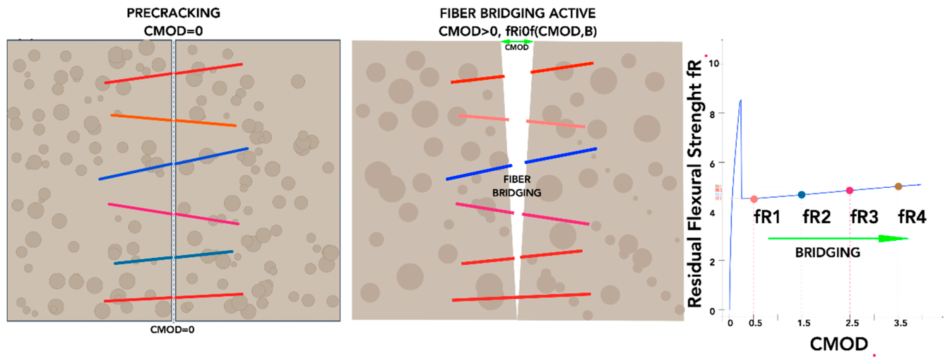
Figure 2.
Distribution plots of primary input features and target variables used in the study, including compressive strength fc, fibre tensile strength fu, fibre geometry parameters, reinforcement index and residual strengths
Figure 2.
Distribution plots of primary input features and target variables used in the study, including compressive strength fc, fibre tensile strength fu, fibre geometry parameters, reinforcement index and residual strengths
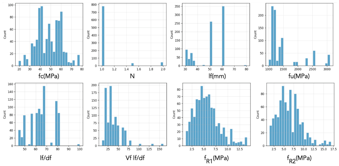
Figure 3.
Predicted vs. Experimental scatter plots for HardPINN.
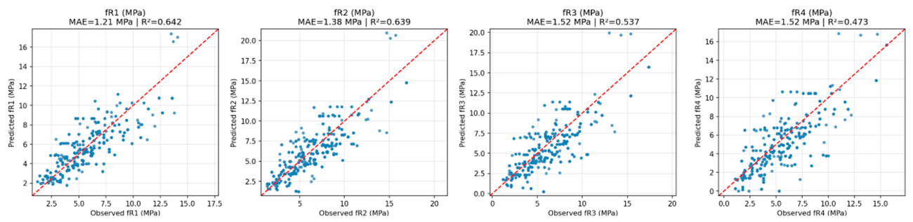
Figure 4.
3 × 4 scatter plot grid comparing HardPINN, RF, and Ridge across all stages.
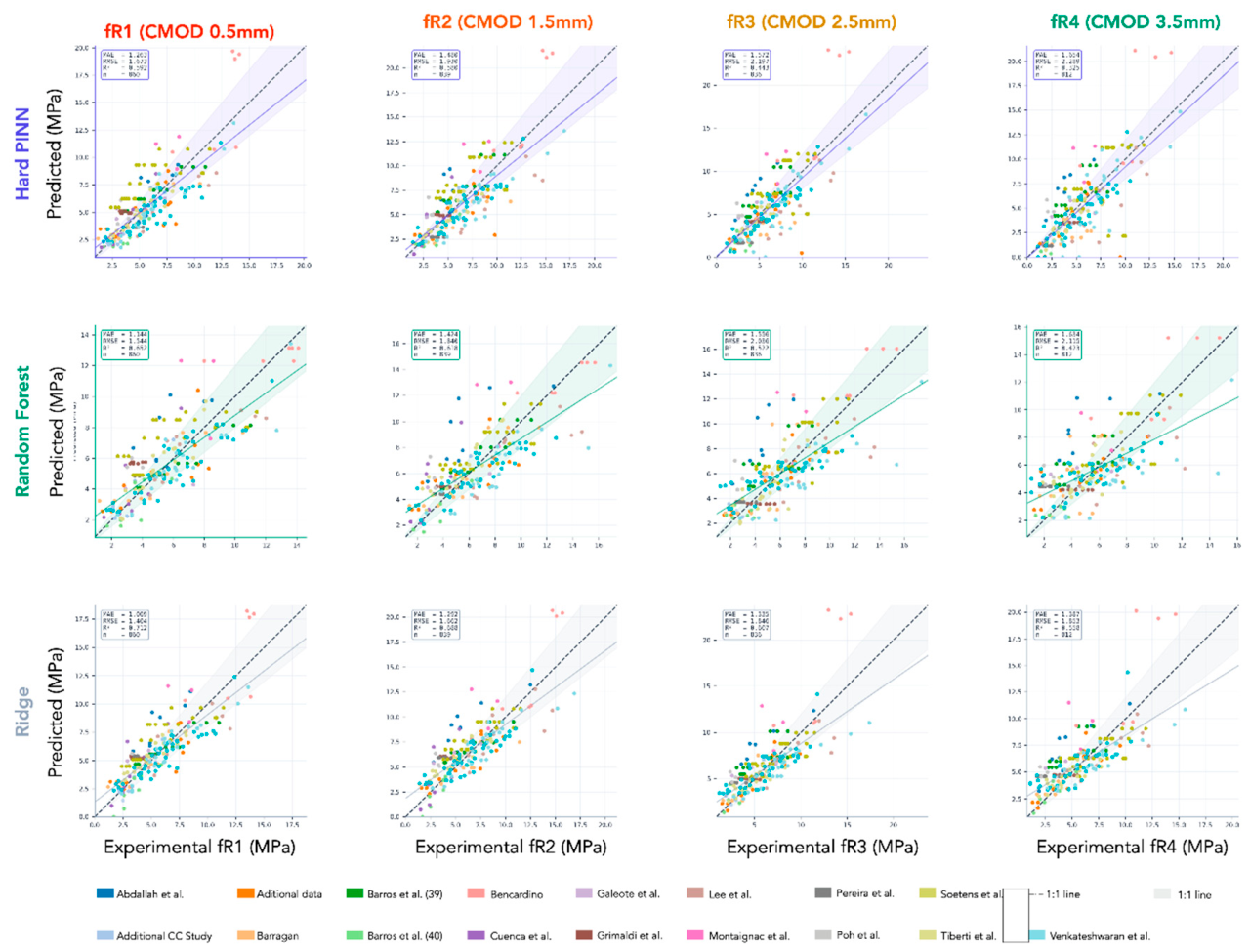
Figure 5.
R2 per fold.
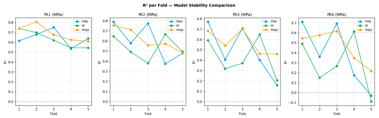
Figure 6.
Correlation scatter plots between RI and fRi. .
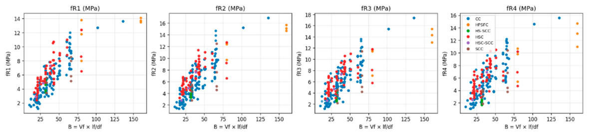
Figure 7.
Study-level prediction error distribution under group-based cross-validation. The hard-constrained PINN exhibits reduced variability across independent experimental datasets.
Figure 7.
Study-level prediction error distribution under group-based cross-validation. The hard-constrained PINN exhibits reduced variability across independent experimental datasets.
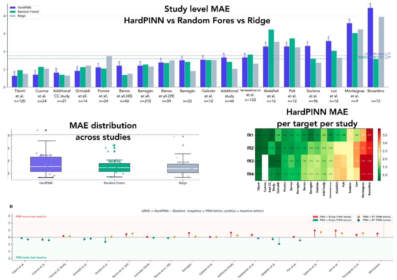

Table 1.
Descriptive statistics of the expanded experimental database (n=860).
| Variable | count | mean | std | min | 25% | 50% | 75% | max |
| fc (MPa) | 860 | 48,331 | 11,605 | 19,2 | 39,7 | 48 | 57,8 | 77,8 |
| N | 860 | 1,073 | 0,241 | 1 | 1 | 1 | 1 | 2 |
| lf (mm) | 860 | 49,424 | 11,321 | 30 | 37 | 50 | 60 | 80 |
| fu (MPa) | 860 | 1499,507 | 575,816 | 1000 | 1160 | 1230 | 1500 | 3100 |
| lf/df | 860 | 64,629 | 10,762 | 44 | 56 | 65 | 67 | 100 |
| Vf × lf/df | 860 | 38,516 | 21,14 | 10,2 | 23,9 | 33,3 | 45,6 | 160 |
| fR1 (MPa) | 860 | 5,649 | 2,62 | 1,2 | 3,775 | 5,3 | 6,9 | 14,1 |
| fR2 (MPa) | 839 | 6,355 | 2,978 | 1,4 | 4,1 | 6,1 | 8,2 | 16,9 |
| fR3 (MPa) | 836 | 6,078 | 2,946 | 1,2 | 3,8 | 5,9 | 8 | 17,4 |
| fR4 (MPa) | 812 | 5,66 | 2,787 | 1,1 | 3,6 | 5,5 | 7,3 | 15,6 |
| Vf (%) | 467 | 0,634 | 0,329 | 0,128 | 0,400 | 0,546 | 0,760 | 2,028 |
| Df (mm) | 467 | 0,790 | 0,158 | 0,375 | 0,746 | 0,769 | 0,923 | 1,200 |
Table 2.
Pearson correlation coefficients between dominant predictors and residual flexural strengths.
Table 2.
Pearson correlation coefficients between dominant predictors and residual flexural strengths.
| Predictor | fR1 | fR2 | fR3 | fR4 |
| fc (MPa) | 0.327 | 0.322 | 0.272 | 0.241 |
| fu (MPa) | 0.198 | 0.250 | 0.284 | 0.290 |
| lf (mm) | 0.026 | 0.142 | 0.178 | 0.214 |
| lf/df | 0.219 | 0.260 | 0.251 | 0.250 |
| RI=Vf(lf/df) | 0.839 | 0.817 | 0.789 | 0.752 |
| log(1+RI) | 0.862 | 0.832 | 0.796 | 0.762 |
| RI x fu | 0.755 | 0.756 | 0.753 | 0.735 |
| RI x fc | 0.834 | 0.813 | 0.775 | 0.732 |
| fu/fc | -0.005 | 0.025 | 0.113 | 0.133 |
Table 3.
Variance Inflation Factor (VIF) values for candidate predictors.
| Predictor | VIF | Diagnosis |
| Group A — Raw physical inputs (baseline) | ||
| (MPa) | 1.21 | Acceptable |
| (MPa) | 1.80 | Acceptable |
| (mm) | 1.47 | Acceptable |
| 1.88 | Acceptable | |
| 1.08 | Acceptable | |
| Group B — Full engineered feature set (used in model) | ||
| (MPa) | 240.84 | Very high |
| (MPa) | 149.52 | Very high |
| (mm) | 1.57 | Acceptable |
| 2.16 | Acceptable | |
| 51.21 | Very high | |
| 12.64 | High | |
| 70.01 | Very high | |
| 336.52 | Very high | |
| 17.22 | High | |
| 39.28 | Very high | |
| 47.36 | Very high | |
Note: Threshold reference: VIF < 5 AcceptableVIF 5–10 ModerateVIF 10–20 HighVIF > 20 Very higBold values: VIF ≥ 10 (high multicollinearity). Shaded rows = features involving reinforcement index RI = Vf×(lf/df). Standardised predictors used to avoid scale-driven inflation. The NonNegDense monotone path in HardPINN isolates RI from the shared backbone, mitigating collinearity effects on gradient updates.\.
Table 4.
Predictive performance of the proposed model across all residual strength targets. Results are reported as mean ± standard deviation over five folds using study-level GroupKFold validation. Metrics include MAE and the r2.
Table 4.
Predictive performance of the proposed model across all residual strength targets. Results are reported as mean ± standard deviation over five folds using study-level GroupKFold validation. Metrics include MAE and the r2.
| fR1 | fR2 | fR3 | fR4 | |
| MAE mean | 1.256 ± 0.531 | 1.514 ± 0.655 | 1.562 ± 0.637 | 1.662 ± 0.659 |
| R2 mean | 0.606 ± 0.170 | 0.538 ± 0.219 | 0.389 ± 0.374 | 0.197 ± 0.480 |
Table 5.
Pooled metrics across all models.
| Model | MAE | R2 | MAE | R2 |
| Ridge | 1.069 | 0.712 | 1.387 | 0.558 |
| Random Forest | 1.144 | 0.652 | 1.634 | 0.423 |
| HardPINN | 1.263 | 0.592 | 1.654 | 0.325 |
Table 6.
Constraint summary.
| Constraint | Mechanism | PINN | RF | Ridge |
| fRi ≥ 0 | softplus/relu floor | 0/3440 (0.00%) | 0/3440* | 0/3440* |
| ∂fRi/∂RI ≥ 0 | NonNegDense | ✓ all 4 targets | Not guaranteed | Not guaranteed |
| |Δi| bounded | BetaTanh | β per target | Not bounded | Not bounded |
| Sequential coherence | Hierarchical heads | Guaranteed | Not guaranteed | Not guaranteed |
*RF and Ridge required post-hoc clipping; PINN is guaranteed by architecture.
Table 7.
Representative predicted residual strengths for selected mixture typologies.
| fc | RI | fu | Type | fR1 | fR2 | fR3 | fR4 |
| 35 | 20 | 1200 | CC | 2.212 | 2.202 | 2.346 | 1.978 |
| 55 | 40 | 1500 | HSC | 5.767 | 7.281 | 7.422 | 6.814 |
| 70 | 60 | 2300 | SCC | 9.730 | 9.637 | 7.536 | 5.647 |
Disclaimer/Publisher’s Note: The statements, opinions and data contained in all publications are solely those of the individual author(s) and contributor(s) and not of MDPI and/or the editor(s). MDPI and/or the editor(s) disclaim responsibility for any injury to people or property resulting from any ideas, methods, instructions or products referred to in the content. |
© 2026 by the authors. Licensee MDPI, Basel, Switzerland. This article is an open access article distributed under the terms and conditions of the Creative Commons Attribution (CC BY) license (http://creativecommons.org/licenses/by/4.0/).
Copyright: This open access article is published under a Creative Commons CC BY 4.0 license, which permit the free download, distribution, and reuse, provided that the author and preprint are cited in any reuse.


