

Submitted:
05 August 2026
Posted:
06 August 2026
You are already at the latest version
Abstract
Electric motorcycles are central to SubSaharan Africa’s transition to electric mobility, yet manufacturers in the region typically rely on costly and time-consuming physical prototyping to optimise powertrains built from imported components. This paper presents a validated full-powertrain digital twin of the Roam Air, an electric motorcycle assembled in Nairobi, Kenya, developed in MATLAB/Simulink as four interconnected subsystems: the battery, the controller, the motor, and the vehicle dynamics. The battery is modelled as a Thévenin equivalent circuit whose parameters were experimentally derived at the pack level through Hybrid Pulse Power Characterisation tests, and the controller replicates the motorcycle’s field-oriented control with a maximum torque per ampere strategy, including its battery current and voltage limiting behaviour. The motorcycle’s regenerative braking characteristics, drag coefficient, and rolling resistance coefficient were experimentally obtained through braking, coasting, and coast-down tests. The digital twin ingests rider inputs and GPS information, and predicts the motor’s speed and the battery’s power. Validation against six measured drive cycles in Stellenbosch, South Africa, demonstrates strong agreement between predicted and measured profiles, with Pearson’s r values of 0.905 0.981 for battery power and 0.912–0.996 for motor speed, and energy consumption predicted to within 2.71% for five of the six trips. The presented modelling and characterisation framework offers manufacturers a transferable, computationally efficient alternative to iterative physical prototyping for powertrain optimisation under Sub-Saharan African operating conditions.
Keywords:
digital twin
; electric motorcycle
; powertrain modelling
; Sub-Saharan Africa
; equivalent circuit model
; field-oriented control
; regenerative braking
1. Introduction
Motorcycles are becoming increasingly popular in Sub-Saharan Africa (SSA), with registrations rising from approximately 5 million in 2010 to around 27 million in 2022 [1]. This is because they improve travel efficiency while providing employment opportunities in passenger transport and delivery services [1]. Motorcycle riders can navigate roads impassable to four-wheeled vehicles, weave through traffic in cities, and bring passengers to their exact destinations [1], offering greater accessibility and shorter travel times. In addition, motorcycles are less expensive to purchase and operate than four-wheeled vehicles, which is favourable to commercial users occupying an estimated 80% of all motorcycles in SSA [1].
Electrifying motorcycles is Africa’s primary move towards electric mobility, as their relatively low mass requires smaller and consequently cheaper battery packs [1]. Electric motorcycles improve local air quality and lower greenhouse gas emissions, noise pollution, and operating costs for riders [1]. According to a survey conducted in nine African cities, electric motorcycle riders spend one third less on weekly energy costs and more than a half less on weekly maintenance costs, compared to petrol motorcycle riders [1]. In South Africa, which has a high-carbon grid, an electric motorcycle is estimated to emit CO2/, compared with CO2/ for an equivalent internal combustion engine motorcycle [2].
Entrepreneurship surrounding electric mobility in SSA include battery pack development, electric motorcycle assembly, and retrofitting electric motorcycles from petrol motorcycles [1]. Electric motorcycle manufacturers in SSA typically import off-the-shelf parts, and design and assemble their motorcycles locally so that they are fit for African operating conditions [3]. Manufacturers typically undergo iterative physical prototyping and empirical testing to optimise their powertrain choices and/or configurations, which is costly and time-consuming [4]. A digital twin provides a more efficient approach to optimising an electric motorcycle’s powertrain, especially for African manufacturers who rely on imported components.
In this paper, a digital twin of an electric motorcycle powertrain is defined as a dynamic virtual replication of the physical powertrain.
The reviewed literature on digital twins of electric vehicle powertrains include [4,5,6]. In [4], the use of a digital twin to predict electric powertrain efficiency (motor and multi-stage transmission efficiency only) is the focus of the study. Various models were assessed to find the best balance of accuracy, prediction speed, and measurement effort [4]. The most complex model, which incorporates machine learning, achieved the best performance [4]. In [5], a virtual environment was created for functional and fault-response testing of electric vehicles, using digital twin technology. The simulation setup combines software (the digital twin simulating the test environment and test scenarios) with hardware (the vehicle control unit (VCU), battery management system (BMS), and motor control unit (MCU)) [5]. In [6], a Modelica library designed to build digital twins of electric powertrains is introduced. The library comprises sub-libraries for the battery, power electronics, and motor, each of which include thermal modelling [6]. The battery sub-library simulates the battery’s electrical behaviour using either an ideal voltage source model, internal resistance model, or resistor-capacitor (RC) element model [6]. The Modelica-built powertrain model was used in conjunction with Ricardo IGNITE (for vehicle dynamics) and MATLAB/Simulink (for the controller and driver models) to simulate the performance of a long-haul truck, yielding successful simulation results [6]. Related literature further includes forward-facing models of electric vehicle powertrains, whereby power calculations flow from a driver model to the vehicle’s wheels [7,8,9]. These models involve a driver model that uses the error between measured drive cycle and observed model speed and a PI controller [7,8,9]. The identified forward-facing models do not simulate the vehicle’s control operations and use simplified battery models [7,8,9]. ADVISOR (Advanced Vehicle Simulator), which is an industry-grade simulator for hybrid electric vehicles, is described in [10]. Backward-facing models calculate the vehicle’s traction force at the wheel from its longitudinal dynamics, and subsequently determine battery power consumption from the wheel [10]. ADVISOR integrates a backward-facing approach (that uses combined inverter-motor efficiency maps) with component variable limits that are characteristic of a forward-facing approach, to strike a balance between accuracy and computational efficiency. ADVISOR demonstrates energy consumption accuracy within 0.6%–1.9% and executes simulations 2.6–8 times faster than representative forward-facing models.
The literature on digital twins for electric vehicle powertrains provides limited methodological detail and places no emphasis on electric motorcycle powertrains. In addition, the identified forward-facing electric powertrain models, which are effectively lower-fidelity digital twins, use an artificial driver model and do not simulate the vehicle’s control operations.
In this paper, a digital twin of an electric motorcycle powertrain is developed, which ingests rider commands (throttle and brake signals) and environmental inputs (road’s gradient and wind speed), employs dynamic powertrain component models (including controller operations implemented on the physical motorcycle), and accurately predicts the motorcycle’s performance (battery power and motor speed). The aim of this paper is to give a comprehensive technical framework on developing a digital twin of an electric motorcycle powertrain, detailing the modelling and experimental characterisation of the powertrain’s components. This is the paper’s primary contribution, which is complemented by the digital twin’s uniqueness of using a more representative driver model and simulating the motor control typically used by electric motorcycles.
2. Theoretical Background
A single-speed electric motorcycle powertrain comprises a battery, motor controller and inverter (which are generally combined in one component), motor, and drivetrain (which include the front and rear sprockets, chain, mechanical brakes, and rear wheel). The motor controller receives rider inputs (throttle or electrical brake signals), supplies low-voltage DC power to the auxiliary components, and drives the motor via the inverter. Mechanical brakes are applied by the motorcycle’s calipers acting on the disc or drum brakes. The combination of mechanical and electrical braking determines the motorcycle’s total braking force. Figure 1 illustrates the interfacing of the electric motorcycle’s powertrain components and the energy flow between them.
The developed digital twin contains dynamic models of the battery, motor controller, and motor. Inverter power losses are obtained from an efficiency map, and the drivetrain gear ratio and friction are accounted for in the motorcycle dynamics.
2.1. Battery
Batteries generally exhibit non-linear characteristics, which complicate the accurate estimation of their equivalent internal resistance, state of charge, and state of health [11]. The battery’s equivalent internal resistance is a function of battery temperature, charge/discharge rate, battery age [11], and state of charge [12].
For Li-ion batteries, there are two classes of models that have been identified in the literature: electrochemical models and equivalent circuit models (ECMs) [11]. Electrochemical models emulate the chemical processes that occur in the battery, whereas ECMs reproduce the battery’s dynamics at a higher abstraction level [11]. Various ECMs have been established, however, the Thévenin and dual polarization (DP) models are commonly used due to their superior dynamic properties [11]. Figure 2 presents the Thévenin and DP ECMs.
When the battery receives a current input, the series resistor () models the instantaneous change in terminal voltage, while the resistor-capacitor (RC) pairs model the dynamic changes in terminal voltage over time. For the DP model, the first RC pair ( and ) represents the faster transient response to a current input, whereas the second RC pair ( and ) represents the slower transient response to a current input [12].
Electrochemical models are numerically complex and computationally heavy [11], and only the current-voltage properties of the battery are of concern for the digital twin; therefore, an ECM is selected for the battery model. Since the DP model includes a second RC pair, its parameter characterisation is more challenging in terms of accuracy and experimental time [12]. Therefore, the digital twin’s battery model uses the Thévenin ECM. For a set sampling time (), the battery’s terminal voltage () is determined from the bus current (I) by
where
2.2. Motor
Motors typically used for electric vehicle applications include direct current (DC) motors, induction motors, brushless DC (BLDC) motors, permanent magnet synchronous motors (PMSMs), and switched reluctance motors (SRMs) [13]. Overall, permanent magnet brushless motors, comprising both PMSMs and BLDC motors, are the dominant choice for electric vehicle propulsion.
A PMSM comprises a stator with copper windings and a rotor with permanent magnets [14]. The PMSM’s stator produces a rotating magnetic field from three-phase alternating currents, which magnetically moves the rotor at the same speed as the stator’s field [14]. PMSMs consist of two types: surface permanent magnet (SPM) motors and interior permanent magnet (IPM) motors (also known as interior PMSMs or IPMSMs), which are characterised by the location of their permanent magnets [14].
Power losses in PMSMs include: stator copper losses, core losses, mechanical losses, and other small miscellaneous losses [14]. Stator copper losses are caused by heating of the stator’s copper windings [14]. Core losses comprise eddy current and hysteresis losses [14]. Eddy current losses result from the resistive heating caused by circulating currents induced in the stator’s core [14]. Hysteresis losses arise from the energy dissipated during the repeated reorientation of the core’s magnetic domains as the magnetic field alternates [14]. Mechanical losses comprise friction and windage losses, caused by movement between the machine’s mechanical components and between these components and the air within the motor casing, respectively [14].
The electrical characteristics of a PMSM can be modelled by the direct-quadrature (dq) model and the finite element method (FEM) [15]. FEM is very accurate and can capture non-linearities caused by hysteresis effects and saturation of the magnetic materials, but FEM is computationally expensive [15]. The dq model is a simpler and computationally efficient approach that enables decoupled torque and flux control, but it relies on assumptions that leads to inaccuracies in performance prediction [15]. For motorcycles that operate using field-oriented control (described further in Section 2.4), the dq model is therefore required, and its voltage equations in the rotor reference frame are defined by
where and are the observed dq voltages, is the motor’s electrical speed, and , , , and is the motor’s stator resistance per phase, dq inductances and permanent magnet flux linkage [14].
2.3. Inverter
The inverter converts DC power from the battery to AC power for the motor, and vice versa. The inverter contributes two main losses to the electric motorcycle system: conduction and switching losses of the inverter’s internal devices [14].
These losses are modelled using an experimentally determined inverter efficiency map, which is an accurate and computationally inexpensive way of dynamically modelling the component’s power losses.
2.4. Controller (Field-Oriented Control)
Field-oriented control (FOC) is typically used for PMSMs. FOC involves independent control of the motor’s torque and flux by transforming the stator’s three-phase quantities into a two-dimensional rotating vector frame (the dq-axis system) [14]. The component of the stator current phasor along the direct axis (d-axis current) can only produce flux, whereas the component of the stator current phasor along the quadrature axis (q-axis current) produces a torque in interaction with the rotor flux [14].
2.4.1. Field-Oriented Control System
FOC, for torque-control, is implemented with a typical closed-loop system as shown in Figure 3 [16,17].
A torque command () enters the control system, from which current commands along the d () and q-axes () are generated according to the control strategy. The dq current commands are then passed through their respective current controllers (which are described further in Section 2.4.2) to produce dq voltage references ( and ). These dq voltage references are converted to three-phase voltages, for motor excitation, via the inverse Park transform:
and the inverse Clarke transform:
The motor’s three-phase currents provide feedback for the PI current regulators after being converted to the dq-axis system via the Clarke transform:
and the Park transform:
The motor’s feedback speed establishes the motor’s operating region (constant-torque or field-weakening). The base speed separates the constant-torque and field-weakening operating regions [14]. As the motor approaches its base speed, the induced electromotive force (EMF) approaches the maximum stator voltage, which is constrained by the DC bus voltage [14]. To enable PMSM operation above the base speed, field-weakening control is employed [14]. In this operating region, the induced EMF is maintained below the maximum available stator voltage by injecting a negative d-axis current, which reduces the motor’s effective air-gap flux linkage [14].
2.4.2. Current Controllers of the Field-Oriented Control System
The current controller regulates the phase currents to ensure accurate tracking of their reference values. The controller is generally a proportional-integrator (PI) type, in which the proportional and integrator gains are based on the per-phase stator resistance and self-inductance of the machine [14]. For interior permanent magnet synchronous motors (IPMSMs), a fully model-based current controller is required in the rotor reference frame [14], which is derived in this section. For a first-order lag system, the transfer function of the current controller is given by
where is the feedback current gain and is the desired lag [14]. In the time domain, Equation (15) becomes
Substituting Equation (16) into the machine equations of a PMSM (Equations 4 and 5) results in
where and are the dq voltage references, and is the inverter gain [14]. Applying the integral to both sides of Equation (16) results in
assuming zero initial conditions. Therefore the PMSM equations become
3. Modelling of Digital Twin
The developed digital twin (DT) is designed to virtually replicate the powertrain of the Roam Air [19], a popular electric motorcycle in Nairobi, Kenya. The DT ingests rider inputs (throttle and brake commands), GPS information (GPS location and altitude), and wind speed data, and outputs the motorcycle’s mobility and battery’s power (as illustrated in Figure 4).
The wind speed data is manually recorded from a smartphone weather application, which provides estimates of both the wind speed magnitude and direction. The GPS information is used to simulate the road’s gradient. After down-sampling the input data (from approximately to 1 ), Gaussian smoothing (with kernel parameters shown in Table 1) is applied to the GPS information before the road’s gradient is calculated. The road’s gradient is calculated from elevation difference () and path length () by
Slope values with are replaced by the nearest slope value with . When , the small values amplify the inaccurate values, leading to irregular slope values. Further slope processing is then performed, whereby slope outliers exceeding the maximum slope of the drive cycle are identified and replaced with the nearest valid slope value. These slope outliers are attributed to random spikes.
The DT was developed in MATLAB/Simulink and its block diagram is shown in Figure 5. The DT comprises four subsystems: 1) the battery, 2) the controller, 3) the motor, and 4) the vehicle’s dynamics. The battery supplies a DC voltage to the controller for vehicle operation. The controller uses the rider’s inputs (throttle and brake commands) and the motor’s feedback signals to control the motor. The motor receives phase voltages (from the controller) and a load torque (based on the vehicle’s dynamics) and returns feedback signals to the controller. The vehicle dynamics subsystem uses environmental information and the motorcycle’s speed to establish the motor’s load torque. Through the interfacing of the subsystems, the DT predicts the motor’s speed and the battery’s power.
3.1. Battery Model
The Thévenin equivalent circuit model (ECM) is implemented using Simulink’s "Battery Equivalent Circuit" block [20]. The battery’s terminal voltage is solved discretely with a sampling frequency of 1 . The bus current is received from the controller model to calculate the battery’s terminal voltage, which is sent to the controller model for the next time instant. For the battery model, the ECM parameters vary according to the battery’s state of charge (SoC) and the flow direction of current as follows:
The ECM’s open-circuit voltage () and parameters (, , ) were experimentally derived at the pack level (Section 4.1) and implemented in a lookup map fashion. The battery’s SoC is determined using the battery’s aged capacity () and the Coulomb counting method [20], which is defined as
Battery temperature and ageing effects on the equivalent internal resistance (EIR) are not modelled due to the difficulty in experimentally obtaining data for empirical modelling or physical modelling validation. The effect of discharge/charge rates on the EIR is also not modelled, but because little ECM parameter variation was observed between the experimental tests with varying discharge/current rates (Section 4.1).
3.2. Controller Model
The Roam Air comprises a controller with specifications described in Table 2. The controller’s inverter efficiency map is shown in Figure 6, which was experimentally determined in [2].
The controller model serves three functions: 1) generating the reference torque, 2) implementing the motorcycle’s motor control, and 3) replicating the motorcycle’s battery current and voltage limits. In addition, the inverter’s power loss is obtained from indexing the efficiency map in Figure 6 with the motor’s operating point. The controller model generates the reference torque with the setup shown in Figure 7.
The "Torque Reference Generator" block produces the reference torque from torque-speed envelopes, feedback motor speed, throttle and brake commands, and the battery’s SoC, using Algorithm 1:
| Algorithm 1: Torque reference generator logic. |
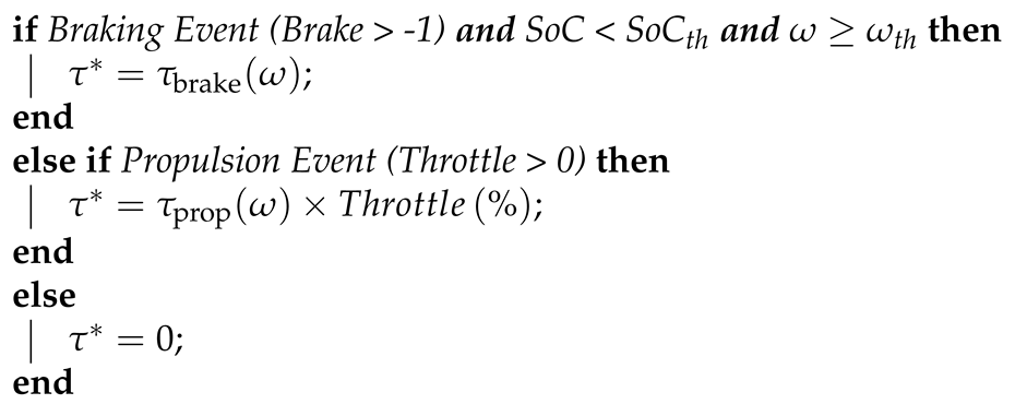 |
The algorithm samples the feedback speed, throttle, and brake inputs at a frequency of 1 . The "Brake" signal is logical (-1 = no brake; 0 = brake), where the transition between the two states is sometimes acknowledged. The "Throttle" signal is a percentage of throttle rotation (0 % = no throttle; 100 % = full throttle). The and values are indexed from their respective torque-speed envelope lookup maps. The torque-speed envelope for propulsion was derived from the motor’s specification sheet [21], whilst the torque-speed envelope for regenerative braking and the and thresholds were experimentally obtained (Section 4.3).
The controller model uses the "Interior PM Controller" block in MATLAB/Simulink to implement FOC in torque control mode [18], with a sampling frequency of 1 . The block uses a MTPA control strategy in the constant-torque operating region, whereby dq current commands are selected such that the required reference torque is produced with the minimum stator current magnitude [14]. The dq currents for MTPA operation ( and ) are determined from
where is the maximum magnitude of the stator current phasor and , and are the motor’s permanent magnet flux linkage and dq inductances.
The controller model performs flux-weakening via the indirect control scheme, in which the negative d-axis current () is analytically determined from
The d-axis current for flux-weakening () is a function of the maximum stator voltage () and the motor’s electrical speed () [14].
In terms of the Roam Air’s flux-weakening algorithm, it is suspected that it follows a simpler adaptive control scheme, which uses the stator voltage error () and a PI control loop to inject a negative d-axis current [14]. This control scheme is different to that implemented in the controller model, however, the Roam Air does not operate in the flux-weakening region. The motorcycle’s specified maximum speed of 90 km/h [19] (3234 rpm) is much less than the motor’s rated base speed (3800 rpm) [21], which is attributed to the motorcycle’s battery current limit set by the controller. This indicates that the motor does not flux-weaken; therefore, the model’s implemented flux-weakening algorithm is never activated and consequently has no influence on the digital twin’s results.
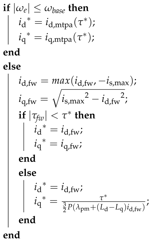
The model’s control logic for the constant-torque and flux-weakening operating regions is outlined in Algorithm 2 [18].
The current commands ( and ) in the constant-torque operating region () are obtained from predetermined lookup tables indexed by the reference torque (). Additionally, the field-weakening d-axis current () is constrained such that the magnitude of the resulting stator current phasor does not exceed the maximum allowable stator current ().
For the PI current controllers that generate the reference dq voltages, a first-order lag system is used (Equation (15)) with the parameters in Table 3.
| Algorithm 2: Control logic for the constant-torque and flux-weakening operating regions. |
 |
The desired lag was selected such that the reference torque, from the throttle signal, is tracked within its 1 s update interval while preventing oscillations in the dq voltage references.
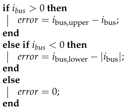
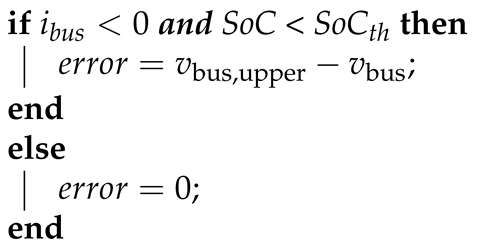
The controller model implements battery current and voltage limiting by dynamically reducing the reference torque via PI control loops that run at a sampling frequency of 1 . The error signals for the battery current and voltage limiting controllers are generated from Algorithms 3 and 4, respectively. The control signals are constrained to only reduce the reference torque when the battery current or voltage exceed their limits. The reference torque is reduced by subtracting or adding the control signal, depending on the sign of the reference torque.
| Algorithm 3: Error signal generation for the battery current limiting controller. |
 |
| Algorithm 4: Error signal generation for the battery voltage limiting controller. |
 |
3.3. Motor Model
The motor model was implemented using the Interior PMSM block in MATLAB/Simulink [22], with a sampling frequency of 1 . It receives the reference phase voltages from the controller model, transforms them to the rotor reference frame to yield and , and calculates the dq currents ( and ) from
where is the stator resistance per phase, is the motor’s electrical speed, is the motor’s mechanical speed, and P is the number of pole pairs. The electromagnetic torque () is then determined from
The motor model then calculates the motor’s speed from
where J is the moment of inertia of the loaded motorcycle, is the Coulomb friction torque of the loaded drivetrain, B is the viscous friction coefficient of the loaded drivetrain, and is the load torque. The calculated dq currents are converted to the stator reference frame and fed back to the controller model, along with the rotor’s mechanical speed and position (). The motor’s stator copper losses () and mechanical losses () are accounted for, and are quantified as power losses from
3.4. Vehicle Dynamics Model
The vehicle dynamics subsystem determines the load torque at the motor () from the external forces exerted on the motorcycle (as shown in Figure 8).
The load force at the wheel () is given by
where is the rolling resistance, is the gravitational force due to the road’s gradient, and is the aerodynamic force, with the equation’s parameters defined in Table 4. The road’s gradient () and wind speed () are obtained from the input data, which is sampled at a frequency of 1 . The motorcycle’s speed () is determined using
where is the motor’s mechanical speed sampled at a frequency of 1 from the motor model, is the drivetrain’s sprocket ratio, and is the rear wheel radius. The load torque at the motor () is given by
The parameters of the vehicle dynamics subsystem are summarised in Table 4.
4. Characterisation of Component Parameters
This section presents the experimental characterisation of the digital twin’s component parameters, covering the battery’s equivalent circuit model (Section 4.1), the motor’s electrical parameters (Section 4.2), the motorcycle’s regenerative braking behaviour (Section 4.3), and the drivetrain’s friction, drag, and rolling resistance coefficients (Section 4.4).
4.1. Battery Tests
The open-circuit voltage-state-of-charge (OCV–SoC) map and equivalent circuit model (ECM) parameters of the Roam Air’s battery pack were obtained experimentally. The specifications of the tested battery pack are presented in Table 5.
Hybrid Pulse Power Characterisation (HPPC) tests were conducted to obtain the ECM parameters, which involve analysing the battery’s terminal voltage response to constant current pulses [12]. The HPPC tests were performed with discharge and charge pulses at 10% state of charge (SoC) increments from 10% to 100%. Undistorted low-current pulses below 10% SoC were difficult to obtain because the battery’s terminal voltage would exceed its lower operating limit (Table 5). At each SoC level, tests with varying current magnitudes within the battery’s operating range (Table 5) were conducted, for both discharge and charge pulses. The intention of this was to investigate the effect of varying discharge and charge rates on the value of the ECM parameters. A pulse duration of 10 s was selected, as this is commonly used for NMC cells [12]. Additionally, the tests were conducted within a battery temperature range of 20 – 40 and each test was repeated five times. Figure 9 shows the experimental setup for the HPPC tests.
The DC power supply was connected to the battery’s terminals and was used to deliver the discharge and charge current pulses. The oscilloscope measured the current pulses and the battery’s terminal voltage, which was visualised and logged (with a sampling frequency of 1 ) on the laptop. Processing of the battery test data was handled in MATLAB, as summarised in Figure 10, which also presents the measured OCV–SoC map.
For the OCV-SoC map, the average terminal voltage, from the beginning of the measurement file to before the first current pulse, was recorded for the different SoC levels. For the ECM parameters, the voltage response during the current pulse was analysed. A moving average filter (with a kernel size of 37 samples) was first applied to the raw voltage data. The theoretical voltage response to a given step current (Equations 1 and 44) was then fitted to the filtered voltage, using a non-linear least-squares solver [23], to obtain the parameters of the Thévenin ECM with one resistor-capacitor pair.
The results of the Thévenin equivalent circuit model (ECM) parameters are described in Figure 11 and Figure 12. Figure 11 shows the effect of current magnitude on the value of the ECM parameters for different states of charge and current directions.
At each state of charge in the six frames, the data points mostly form dense clusters, indicating little change in the ECM parameter values for varying current magnitudes. The red data points (representing the 10 A current pulses) and sometimes the green data points (representing the 20 A current pulses) are more dispersed, possibly due to their lower signal-to-noise ratio, which influences the curve-fitting. Consequently, the ECM results from the 40 A current pulses were selected for the battery model, which are more robust to noise and SoC drift.
During the experimental tests, distortion of current pulses greater than 20 A occurred at SoC levels of 10% and 100%, for discharge and charge pulses respectively. Consequently, the ECM parameter results from the 20 A pulses were used at 10% SoC for discharging and 100% SoC for charging.
The ECM results from repeated measurements were averaged after the removal of outliers. Figure 12 presents the average ECM results and their individual measurements for discharge and charge pulses across the SoC range.
The ECM results are similar across the SoC range, except for the and results at 10% SoC. This is consistent with the OCV-SOC slope between 10% SoC and 22% SoC (Figure 10(a)), whereby the faster decline in open-circuit voltage contributes towards the differently behaving battery during the current pulse.
4.2. Motor Characterisation
The Roam Air uses a single motor with specifications presented in Table 6.
The stator resistance per phase (), direct-quadrature (dq) inductances ( and ), and permanent magnet flux linkage () were determined from a DC test, locked rotor test, and back-EMF test, respectively. The DC test involves injecting a small DC current between two of the motor’s phases, measuring the line-to-line resistance (), and calculating the phase resistance () from
The locked rotor test involves mechanically locking the rotor at a specific angle, injecting a low frequency AC voltage into the stator windings, measuring the current response, and calculating the required parameter. To determine , the rotor is aligned with the d-axis, which is parallel to the magnetic axis of any pole pair. To determine , the rotor is aligned with the q-axis, which is electrically perpendicular to the d-axis. The dq inductance values (L) are calculated from
where is the motor’s electrical speed, V is the root mean square (RMS) value of the applied stator phase voltage, and I is the RMS value of the measured stator phase current.
The back-EMF test involves spinning the motor without current, measuring the RMS line-to-line back-EMF (), and calculating the permanent magnet flux linkage () from
The resulting parameter values of the dq motor model are shown in Table 7.
4.3. Regenerative Braking Assessment
Rudimentary experiments were conducted to quantify the effect of speed, battery SoC, and inertia on the motorcycle’s regenerative energy, for both braking and coasting events. The experiments involved decelerating the motorcycle from certain speeds through braking or coasting, whilst only changing one variable (speed, battery SoC, and inertia). Timestamped battery voltage, battery current, and motor speed were recorded by the motorcycle’s onboard telemetry system to indicate the motorcycle’s regenerative energy and determine the regenerative torque from Newton’s 2nd Law (Equation (35)). At each initial speed, the regenerative torque was determined from the samples collected between the initial speed and 5 / below the initial speed.
To determine the effect of speed on the motorcycle’s regenerative energy, the effect of battery SoC and inertia were controlled by using battery packs with a sufficiently low SoC (SoC ≤ 70%) and keeping the motorcycle’s payload constant. Coasting and braking tests were then performed at initial speed increments of 10 km/h from 10 km/h to 80 km/h, with between 5 and 43 repetitions for each initial speed.
To determine the effect of battery SoC on the motorcycle’s regenerative energy, the tests were performed at initial speeds of 40 km/h. Four different batteries were used for these tests, each with SoC values of 70%, 80%, 90%, and 95%. This SoC range was selected based on observations from the motorcycle’s driving cycle data, whereby no regeneration occurs between 100% and 95% and maximum regeneration occurs from 80% and below.
To determine the effect of inertia on the motorcycle’s regenerative energy, the tests were performed with an added passenger at initial speeds of 40 km/h and a battery pack with a sufficiently low SoC.
Figure 13 displays the empirically derived relationship between speed and regenerative torque, which is averaged from the results of the individual measurements at each speed. These results pertain to braking events as it was discovered that no regeneration occurs for coasting events.
The regenerative torque appears to be fairly constant at approximately -17 Nm across the speed range. The minimum speed of regeneration was assumed to be 10 km/h due to difficulty in conducting tests below 10 km/h. This observation is consistent with the constant-torque region of the regenerative torque-speed envelope of a typical interior permanent magnet synchronous motor (IPMSM) [14]. This is further supported by the fact that the motorcycle does not enter the flux-weakening operating region (Section 3.2).
Figure 13 illustrates the observed relationship between battery SoC and the regenerative current, expressed as a percentage of the maximum regenerative current, measured from initial speeds of 40 km/h.
Above 95% SoC, the controller disallows regenerative braking. Between 95% SoC and 80% SoC, the controller permits regenerative braking which is battery voltage limited. At 80% SoC and below, the maximum regenerative current at 40 km/h is attainable.
After comparing the regenerative battery current for different motorcycle payloads, it was concluded that the motorcycle’s inertia has no effect on its regenerative capability.
4.4. Coast-Down Tests
In this paper, coast-down tests involve decelerating the motorcycle from full speed to rest, without applying brakes, to derive properties of the motorcycle from its speed profile. Two variations of the coast-down test were performed: 1) with an unloaded drivetrain to obtain the drivetrain’s Coulomb friction torque () and viscous friction coefficient (B), and 2) with a loaded drivetrain to obtain the drag and rolling resistant coefficients ( and ).
The unloaded drivetrain coast-down test was first conducted by lifting the motorcycle’s rear wheel using its stand. The test was repeated 15 times with all repetitions demonstrating similar measured speed profiles as shown in Figure 14.
Due to the linearity of the speed profile, it is assumed that the viscous friction of the drivetrain is negligible. Consequently, the average deceleration of the motor within the linear region of the speed profile () was used to calculate the Coulomb friction torque of the drivetrain () from
The effective inertia of the drivetrain () was approximated by determining the individual inertias of the drivetrain’s rotary components, specifically the rear wheel, chain, sprockets, and the motor’s rotor. The calculated Coulomb friction torque represents that of the loaded motorcycle in the digital twin despite being determined from the unloaded motorcycle. However, any difference from the calculated value is captured in the rolling resistance coefficient () determined from the loaded drivetrain coast-down test.
The loaded drivetrain coast-down test was conducted on a paved test section. The test was performed for different rider conditions (upright single rider, low-drag single rider, and upright rider and passenger), and each test was repeated between 4 and 6 times in each direction. A typical profile of the measured speed from the loaded drivetrain coast-down test is shown in Figure 14.
The drag and rolling resistance coefficients were determined by fitting a linear model to the measured deceleration of the motor () using the least-squares method [24]. From Newton’s 2nd Law (Equation (35)), the following linear model was derived:
where is the motorcycle’s speed in m/s, and , , A, , J, m, g, and is the rear wheel radius, air density, frontal area, sprocket ratio, effective inertia of the loaded motorcycle, loaded motorcycle mass, acceleration due to gravity, and the unloaded drivetrain’s Coulomb friction torque.
Table 8 presents the Coulomb friction torque, drag coefficient, and rolling resistance coefficient values obtained from the coast-down tests.
The estimated Coulomb friction torque and rolling resistance coefficients exhibit high repeatability, as indicated by their low standard deviations obtained from 15 and 8 measurements, respectively. The drag coefficient results demonstrate higher standard deviations, which are attributed to variations in wind speed and rider posture during each test.
For comparison, Coulomb friction torque values were difficult to obtain from literature. However, the identified drag and rolling resistance coefficients align with values reported in literature. A typical rolling resistance coefficient used for passenger cars on concrete is 0.015 [25], which is expected to be higher than the empirically-derived coefficients of the motorcycle on asphalt. In [26], computational fluid dynamics was performed on a sports motorcycle, whereby a drag coefficient of 0.53 was obtained for the rider in the upright position. The Roam Air is not fully-faired like a sports motorcycle, and so its drag coefficient is expected to be higher.
5. Results
This section presents the validation results of the digital twin against the six measured drive cycles, covering the battery model’s terminal voltage predictions and the digital twin’s predictions of battery power, motor speed, and energy consumption.
5.1. Validation of Digital Twin
The digital twin is validated against measured driving cycle data generated in Stellenbosch, South Africa. The driving cycle data covers a variety of riding and environmental conditions, which is summarised in Table 9.
To distinguish between electrical braking (which is activated by the initial brake lever movement) and mechanical braking (which engages after a greater lever displacement), a sensor measuring the brake lever’s angular displacement about its pivot point would be required. Since retrofitting such a sensor to the motorcycle was beyond the scope of this work, mechanical braking inputs were not incorporated into the digital twin. Consequently, the validation dataset was generated using only electrical braking. Figure 15 illustrates the validation process of the digital twin.
5.2. Battery Model Results
The battery model is validated against the measured battery terminal voltage of the driving cycle data described in Table 9. Figure 16 and Table 10 present the battery model’s results .
From observing the profiles as well as the Pearson’s correlation coefficient (r), it is evident that the predicted voltage profile strongly follows the measured profile. The associated p-values of Pearson’s r are not reported, as consecutive samples within a drive cycle are highly autocorrelated, which violates the independence assumption underlying the standard significance test for Pearson’s r. Furthermore, the error metrics (MAE, RMSE, and NRMSE) indicate little deviation from the measured voltage for most trips (2, 3, 5, and 6), whilst the other trips (1 and 4) demonstrate moderate errors.
For trips 1 and 3, there appears to be a noticeable offset between the predicted and measured profiles. For trip 1, the profiles have similar shapes, with the predicted profile shifted upwards. This is possibly due to an error in the initial condition. The offset in trip 3 also originates from an initial condition error, which is exacerbated by the mismatch at the rising and falling edges of the peaks. This may be attributed to differing battery temperatures during test and validation data generation.
5.3. Digital Twin Results
Table 11 compares the digital twin’s predicted energy consumption with the motorcycle’s measured energy consumption, for the six drive cycles described in Table 9. Figure 16 and Table 10 present the results of the battery power and motor speed predicted by the digital twin.
In terms of predicted energy consumption per trip, the digital twin produces percentage errors within -1.05% and 2.71% for trips 1, 2, 3, 5, and 6 (Table 11). Trip 4 exhibits a moderate percentage error of 10.65%, however, this percentage error is amplified by the low measured consumption of the trip.
The predicted battery power and motor speed profiles are of similar shape to their respective measured profiles (Figure 16). This is further supported by their similarity metrics (Table 10), demonstrating strong positive correlations with Pearson’s r values of 0.905–0.981 for battery power and 0.912–0.996 for motor speed. The battery power error metrics (MAE, RMSE, and NRMSE) indicate little errors for trips 1, 2, 3, 5, and 6, which have average errors of less than 10% of the trip’s measured power range (NRMSE). These trips primarily contain full-throttle and hard electric braking events, whereas Trip 4 contains rapid throttle fluctuations that make torque request interpretation more challenging. Therefore, considering the characteristic of trip 4’s drive cycle and its profile in Figure 16, the digital twin performs reasonably well for trip 4, despite its moderate error metrics. Additionally, from Trip 1’s battery power profile, it appears that the digital twin underestimates regenerative power. These underestimations align with the large discrepancies in trip 1’s motor speed profile, which is likely affected by poor environmental modelling.
5.4. Discussion of Results
The digital twin’s overall accuracy compares favourably with existing electric vehicle powertrain models in the literature, despite the added complexity of simulating a motorcycle’s field-oriented control and battery current/voltage limiting behaviour rather than relying on a simplified driver model. The energy consumption error of within 2.71% for five of the six trips is comparable to the 0.6–1.9% accuracy reported for ADVISOR [10], a mature, industry-grade simulator. This suggests that the additional modelling detail incorporated in the digital twin, particularly the replication of the motorcycle’s actual field-oriented control and battery limiting logic, has not come at the expense of predictive accuracy.
A common thread runs through the three trips that exhibited the largest deviations from measured data (trips 1, 3, and 4). In each case, the discrepancy was attributed to a variable that was not independently measured during validation: differing battery temperature (trip 3) and wind speed (trip 1), or to a system behaviour, throttle modulation (trip 4), that is inherently more difficult to capture in a physics-based model regardless of input quality. This points to a specific and addressable limitation of the present validation exercise, rather than a shortcoming of the underlying component models themselves. The battery model, motor model, and vehicle dynamics model were each independently and rigorously characterised (Section 4), and their errors during validation are plausibly driven by unmeasured or assumed environmental conditions rather than by deficiencies in the characterised parameters. Future validation work that measures wind speed directly at the vehicle, rather than relying on smartphone weather-application estimates, and that instruments battery temperature directly, would help to isolate the digital twin’s irreducible modelling error from error introduced by incomplete input data.
From a practical standpoint, the level of accuracy demonstrated here, energy consumption predicted to within 2.71%, and battery power and motor speed tracked with Pearson’s r values above 0.9 in all cases, is likely sufficient to support the kind of comparative powertrain decisions (e.g. battery pack sizing, motor selection, gear ratio choice) that motivate this work. Manufacturers are typically interested in the relative performance of candidate configurations rather than absolute precision, and the digital twin’s demonstrated fidelity supports this use case even without further refinement. However, the exclusion of mechanical braking from the validation dataset (Section 5.1) means this accuracy has only been demonstrated under electrical-only braking conditions, and manufacturers relying on the digital twin for range or energy-consumption predictions under real-world riding, which mixes mechanical and electrical braking, should treat the reported accuracy as an upper bound until this is addressed.
Beyond the input-data limitations discussed above, several simplifications in the component models themselves are worth noting. The motor model accounts for stator copper losses but not core losses (eddy current and hysteresis losses), which are typically smaller than copper losses at the motor’s rated operating point but may introduce additional unmodelled error at higher electrical frequencies. Similarly, the battery model uses a single resistor-capacitor pair rather than the dual polarisation model described in Section 2.1, trading some transient accuracy for a simpler and more tractable characterisation process; the strong agreement between predicted and measured terminal voltage (Table 10) suggests this trade-off was reasonable for the drive cycles tested, though it may understate transient behaviour under more aggressive current profiles than those captured here. No thermal modelling is included for either the battery or the motor, which is consistent with the digital twin’s intended use for powertrain configuration decisions over short drive cycles, but would need to be addressed before the digital twin could be used to predict long-term performance degradation or behaviour under sustained high-load conditions.
These simplifications shape where the digital twin is best applied. The validated drive cycles span flat, uphill, downhill, high-speed, and low-speed conditions, as well as single-rider and two-rider payloads, and the digital twin performs consistently well across all of these, supporting its use for performance prediction under representative Sub-Saharan African riding conditions. Its use for comparing powertrain configurations, differing battery capacities, motor specifications, or drivetrain gear ratios, follows directly from the component-level, physics-based structure of the model, since each subsystem can be reparametrised independently. The evaluation of alternative motor control strategies is a plausible further use case given that the controller is modelled as a distinct subsystem, though this has not been validated in the present work and would require its own experimental characterisation before the results could be trusted.
6. Conclusions
This paper presented a validated full-powertrain digital twin of the Roam Air electric motorcycle, developed to support powertrain optimisation for electric motorcycle manufacturers operating in Sub-Saharan Africa. The digital twin models the battery, motor controller, motor, and vehicle dynamics as interconnected subsystems in MATLAB/Simulink, and ingests rider telemetry and GPS data to predict battery power and motor speed during real-world drive cycles.
The powertrain’s component parameters were characterised through three experimental programmes. HPPC testing of the NMC battery pack yielded a Thévenin ECM whose parameters are consistent across the operating SoC range, with the exception of the RC pair resistance and time constant at 10% SoC, which is attributed to the steeper OCV decline in that region. Regenerative braking experiments revealed that the motorcycle produces an approximately constant regenerative torque of -17 Nm across the braking speed range, that regeneration is permitted below 95% SoC with battery voltage limiting activated for voltages exceeding the battery’s upper limit, and that vehicle payload has no discernible effect on regenerative capability. Coast-down testing yielded a Coulomb friction torque of 2.17 Nm, a drag coefficient of 0.61–0.68 depending on rider posture, and a rolling resistance coefficient of approximately 0.01 on asphalt, all of which are consistent with values reported in the literature for comparable vehicles.
The digital twin was validated against six drive cycles covering a range of riding and environmental conditions in Stellenbosch, South Africa, over which the battery model tracked the measured terminal voltage closely, with Pearson’s r values of 0.90–0.97 and NRMSE values of 0.085–0.174. The digital twin predicts battery power and motor speed with strong fidelity, achieving Pearson’s r values of 0.905–0.981 for battery power and 0.912–0.996 for motor speed, and reproduces energy consumption to within 2.71% for five of the six trips. Trip 4, a short downhill segment with rapid throttle fluctuations, exhibited a higher percentage error of 10.65%, which is attributable in part to the low absolute energy consumption of that trip amplifying percentage deviations, and to the model’s limited ability to capture rapid transient throttle behaviour.
The principal limitation of the present work is the exclusion of mechanical braking from the validation dataset, necessitated by the inability to distinguish electrical from mechanical braking in the available telemetry. In addition, battery temperature and ageing effects on the equivalent internal resistance are not modelled, and wind speed during validation was approximated rather than directly measured. Future work should incorporate a brake lever displacement sensor to enable full braking characterisation, and should investigate the sensitivity of the digital twin’s predictions to temperature variation and battery degradation over the operational life of the motorcycle. The methodology and experimental characterisation framework presented here are transferable to other electric motorcycle platforms operating in similar contexts across Sub-Saharan Africa, and provide a foundation for computationally efficient powertrain optimisation without the need for repeated physical prototyping.
Author Contributions
Conceptualization, M.J.B.; methodology, H.A., S.B., M.J.B.; software, H.A.; validation, S.B., M.J.B.; formal analysis, H.A., S.B., M.J.B.; investigation, H.A., S.B., M.J.B..; resources, S.B., M.J.B.; data curation, H.A.; writing—original draft preparation, H.A.; writing—review and editing, S.B., M.J.B.; visualization, H.A., M.J.B.; supervision, S.B., M.J.B.; project administration, M.J.B.; funding acquisition, M.J.B. All authors have read and agreed to the published version of the manuscript.
Funding
This research received financial support from the Western Cape Government Motorised Transport (WC GMT), contract number S009285, and Catalytic Finance through the Subnational Climate Fund, contract number S010624.
Data Availability Statement
The data presented in this study are available on request from the corresponding author.
Acknowledgments
Acknowledgement and appreciation are extended to Roam for providing their motorcycle and data, and to colleagues in the Electric Mobility Lab at Stellenbosch University for their experimental support.
Conflicts of Interest
The authors declare no conflicts of interest.
References
- Bishop, T.; Courtright, T. The Wheels of Change: Safe and Sustainable Motorcycles in Sub-Saharan Africa; FIA Foundation, 2022; Available online: https://www.fiafoundation.org/resources/the-wheels-of-change-safe-and-sustainable-motorcycles-in-sub-saharan-africa (accessed on 26 June 2026).
- Adams, H.; Botha, S.; Booysen, M.J. A Validated Physics-Based Powertrain Model for an Electric Motorcycle in Sub-Saharan Africa. World Electr. Veh. J. 2026, 17, 90. [Google Scholar] [CrossRef]
- Payton, B. EV Manufacturing Shows Signs of Promise in Africa. African Business. 2024. Available online: https://african.business/2024/07/trade-investment/ev-manufacturing-shows-signs-of-promise-in-africa (accessed on 26 June 2026).
- Kopp, L.; Ockert, N.; Cadau, L.; Kley, M. Development of a Digital Twin of a Powertrain for Efficiency Estimations with Machine Learning and Physical Modeling. Adv. Model. Simul. Eng. Sci. 2026, 13, 13. [Google Scholar] [CrossRef]
- Li, C.; Lei, J.; Yang, L.; Xu, W.; You, Y. Research on Electric Vehicle Powertrain Systems Based on Digital Twin Technology. Electronics 2024, 13, 4103. [Google Scholar] [CrossRef]
- Fotias, N.; Bao, R.; Niu, H.; Tiller, M.; McGahan, P.; Ingleby, A. A Modelica Library for Modelling of Electrified Powertrain Digital Twins. In Proceedings of the Proceedings of the 14th International Modelica Conference, Linköping, Sweden, 2021; pp. 249–261. [Google Scholar]
- Zhou, S.; Truong, D.Q.; Zhu, T.; Kirca, M.C.; McGordon, A. Impact of riding posture and regenerative braking on electric motorcycle energy consumption. In Proceedings of the IEEE Conference on Vehicle Power and Propulsion (VPPC); IEEE, 2024. [Google Scholar]
- Adegbohun, F.; Von Jouanne, A.; Phillips, B.; Agamloh, E.; Yokochi, A. High performance electric vehicle powertrain modeling, simulation and validation. Energies 2021, 14, 1493. [Google Scholar] [CrossRef]
- Yuniarto, M.N.; Wiratno, S.E.; Nugraha, Y.U.; Sidharta, I.; Nasruddin, A. Modeling, simulation, and validation of an electric scooter energy consumption model: A case study of indonesian electric scooter. IEEE Access 2022, 10, 48510–48522. [Google Scholar] [CrossRef]
- Wipke, K.B.; Cuddy, M.R.; Burch, S.D. ADVISOR 2.1: A user-friendly advanced powertrain simulation using a combined backward/forward approach. IEEE Trans. Veh. Technol. 1999, 48, 1751–1761. [Google Scholar] [CrossRef]
- Laadjal, K.; Cardoso, A.J.M. Estimation of Lithium-Ion Batteries State-Condition in Electric Vehicle Applications: Issues and State of the Art. Electronics 2021, 10, 1588. [Google Scholar] [CrossRef]
- Białoń, T.; Niestrój, R.; Skarka, W.; Korski, W. HPPC Test Methodology Using LFP Battery Cell Identification Tests as an Example. Energies 2023, 16, 6239. [Google Scholar] [CrossRef]
- Pravallika, G.; Sujatha, P.; Kumar, P.B. Different traction motor topologies with lithium-air battery for electric vehicles: A review. Mater. Today Proc. 2023. [Google Scholar] [CrossRef]
- Krishnan, R. Permanent Magnet Synchronous and Brushless DC Motor Drives; CRC Press, 2017. [Google Scholar]
- Azom, M.A.; Hossain, M.S.; Khan, M.Y.A. Review of electrical and thermal modeling techniques for three-phase PMSM drives. Control Syst. Optim. Lett. 2025, 3, 75–83. [Google Scholar] [CrossRef]
- Carter, S.B.R.; Praveen, P.; Varadhan, N.S.V.; Kowshik, S.; Gopinath, G. Field-Oriented Control (FOC) for Permanent Magnet Synchronous Motors (PMSM) in Electric Vehicle. In Proceedings of the 2023 International Conference on Next Generation Electronics (NEleX); IEEE, 2023; pp. 1–5. [Google Scholar]
- Ramesh, P.; Umavathi, M.; Bharatiraja, C.; Ramanathan, G.; Athikkal, S. Development of a PMSM Motor Field-Oriented Control Algorithm for Electrical Vehicles. Mater. Today Proc. 2022, 65, 176–187. [Google Scholar] [CrossRef]
- MathWorks. Interior PM Controller. 2026. Available online: https://www.mathworks.com/help/autoblks/ref/interiorpmcontroller.html (accessed on 2026-06-18).
- Roam Electric. Motorcycles. 2026. (accessed on 2026-07-12).
- MathWorks. Battery Equivalent Circuit. 2026. Available online: https://www.mathworks.com/help/simscape-battery/ref/batteryequivalentcircuit.html (accessed on 2026-06-17).
- Motor, Q.S. QS138 3000W QSD138A-70 Motor V1 Electric Mid Drive Motor. 2026. Available online: https://www.cnqsmotor.com/product/qs138-3000w-qsd138a-70-motor/ (accessed on 26 June 2026).
- MathWorks. Interior PMSM Block — Dynamic Model of a Three-Phase Interior Permanent Magnet Synchronous Machine Used for Simulation and Control Development. 2026. Available online: https://www.mathworks.com/help/autoblks/ref/interiorpmsm.html (accessed on 2026-06-24).
- MathWorks. lsqcurvefit—Solve Nonlinear Curve-Fitting (Data-Fitting) Problems in Least-Squares Sense. 2026. Available online: https://www.mathworks.com/help/optim/ug/lsqcurvefit.html (accessed on 26 June 2026).
- MathWorks. polyfit—Polynomial Curve Fitting. 2026. Available online: https://www.mathworks.com/help/matlab/ref/polyfit.html (accessed on 26 June 2026).
- Gillespie, T.D. Fundamentals of Vehicle Dynamics; SAE International: Warrendale, PA, USA, 2021. [Google Scholar]
- Wiński, K.; Piechna, A. Comprehensive CFD Aerodynamic Simulation of a Sport Motorcycle. Energies 2022, 15, 5920. [Google Scholar] [CrossRef]
Figure 1.
Block diagram of an electric motorcycle powertrain. Source adapted from [2].
Figure 1.
Block diagram of an electric motorcycle powertrain. Source adapted from [2].
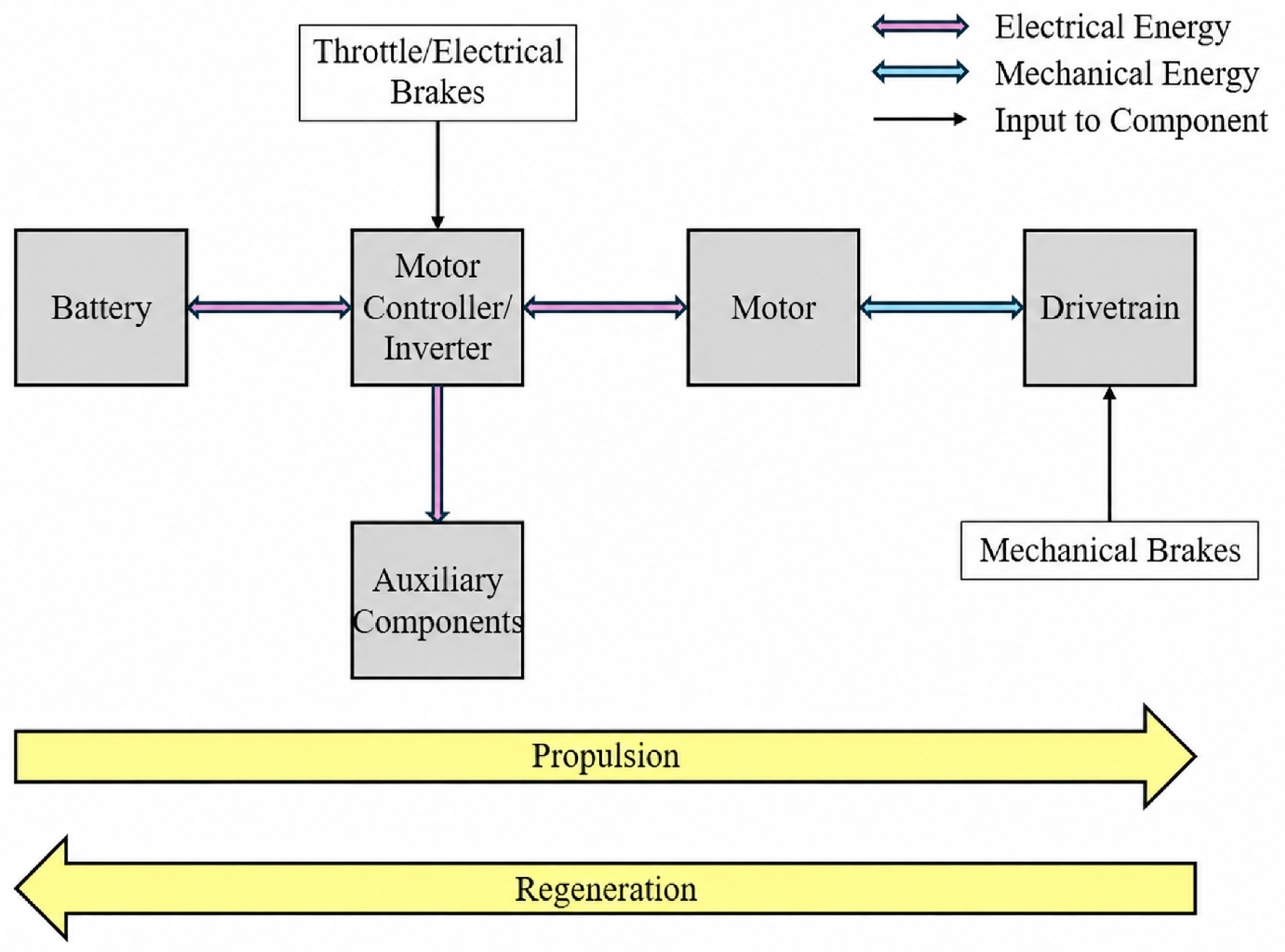
Figure 2.
Battery equivalent circuit models.
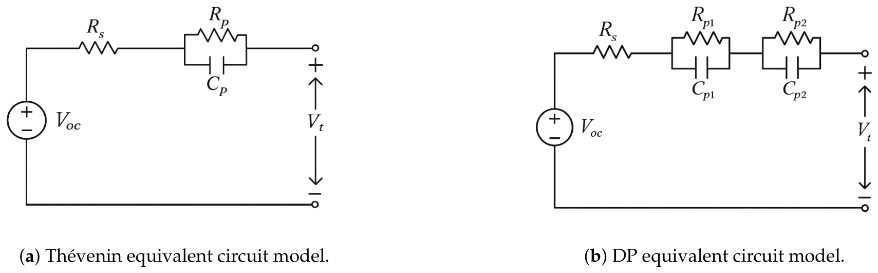
Figure 3.
FOC closed-loop system. Source adapted from [18]
Figure 3.
FOC closed-loop system. Source adapted from [18]
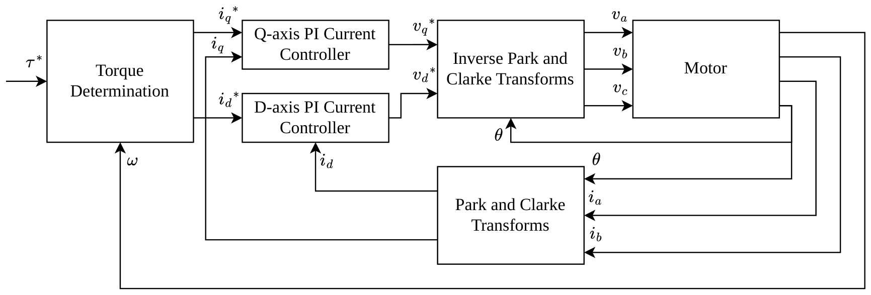
Figure 4.
Simulation setup. (a) High-level simulator overview: information from smartphone weather application (yellow), raw telemetry data (green), processed inputs of digital twin (orange), and outputs of digital twin (blue). (b) Preprocessing of GPS information to determine the road’s gradient.
Figure 4.
Simulation setup. (a) High-level simulator overview: information from smartphone weather application (yellow), raw telemetry data (green), processed inputs of digital twin (orange), and outputs of digital twin (blue). (b) Preprocessing of GPS information to determine the road’s gradient.
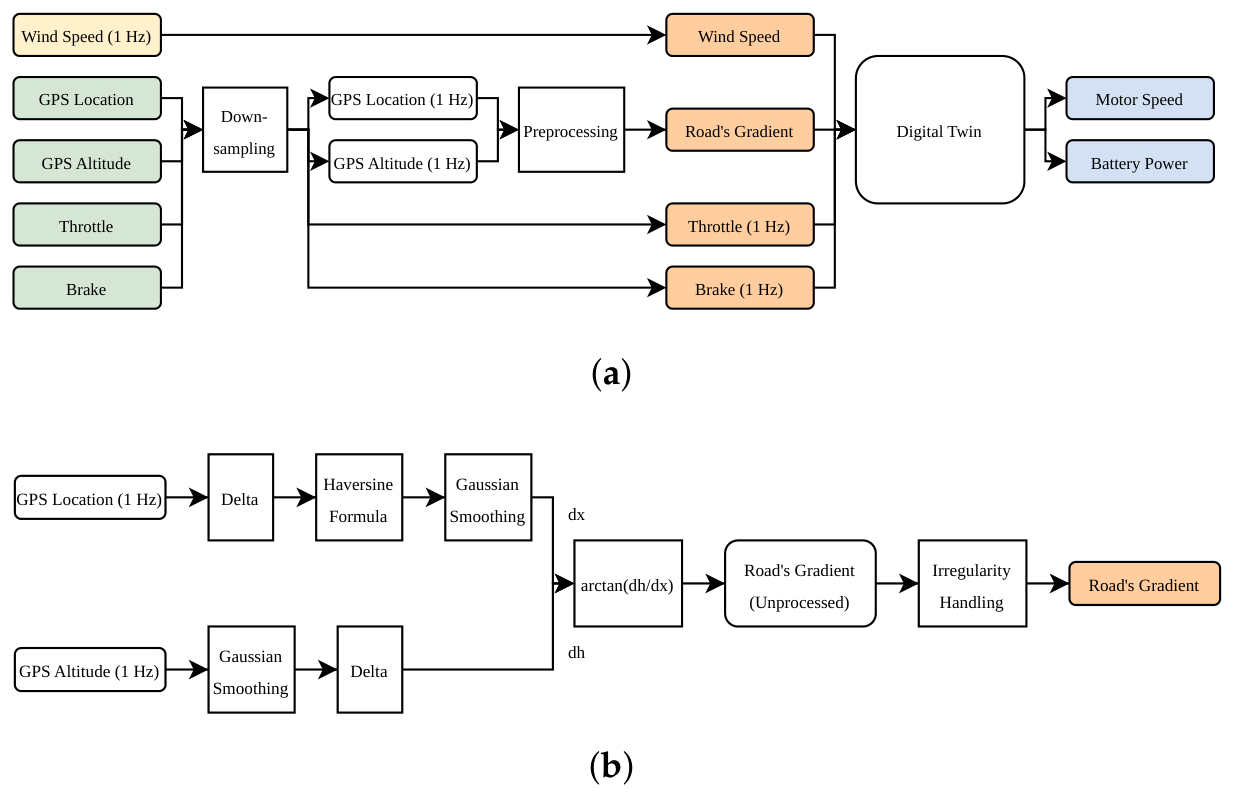
Figure 5.
Digital twin’s Simulink block diagram: processed inputs of digital twin (orange) and outputs of digital twin (blue).
Figure 5.
Digital twin’s Simulink block diagram: processed inputs of digital twin (orange) and outputs of digital twin (blue).
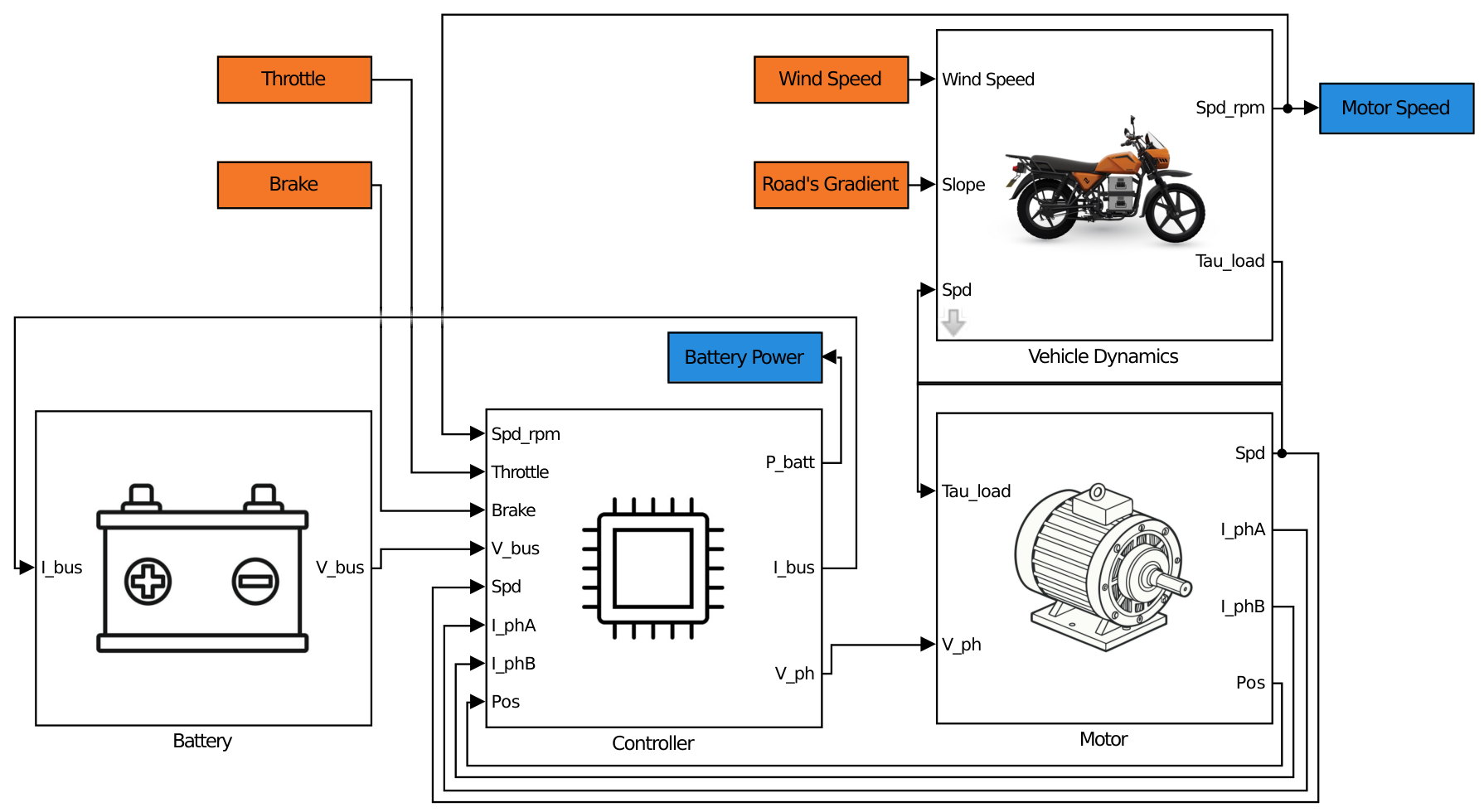
Figure 6.
Experimentally determined efficiency map of the Roam Air’s inverter.
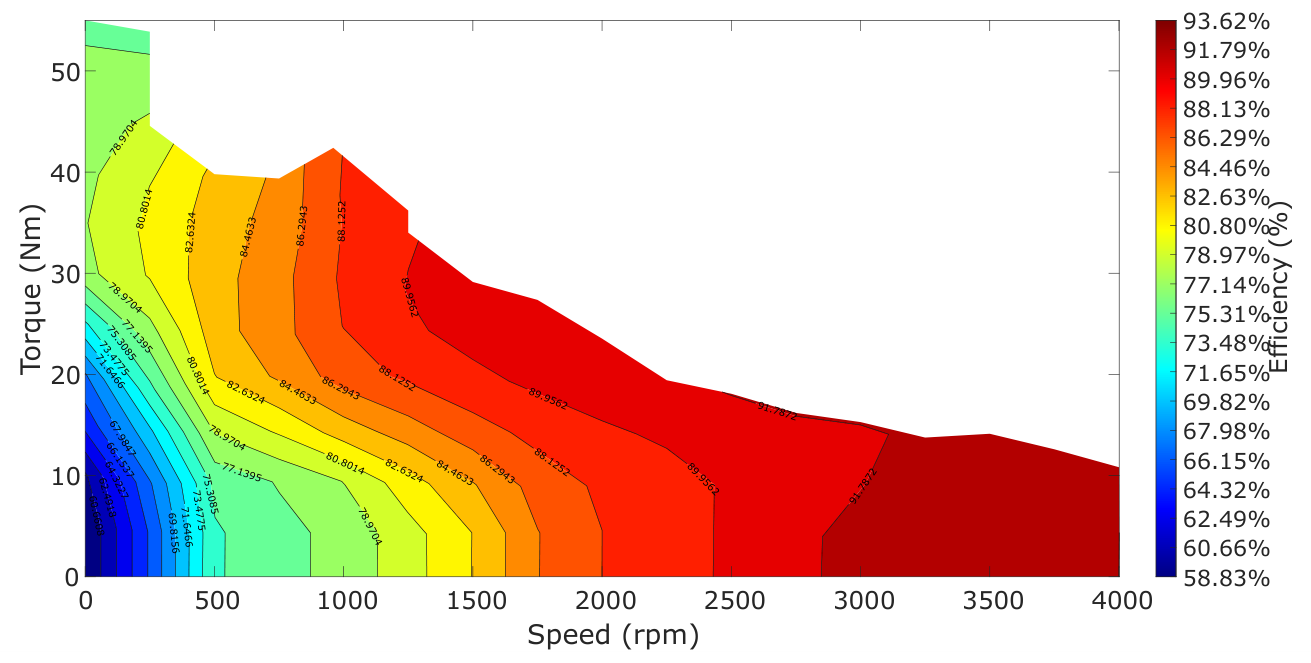
Figure 7.
Controller model’s reference torque generation.
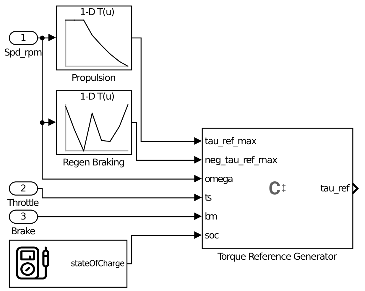
Figure 8.
Free-body diagram showing the predominant external forces exerted on the motorbike.
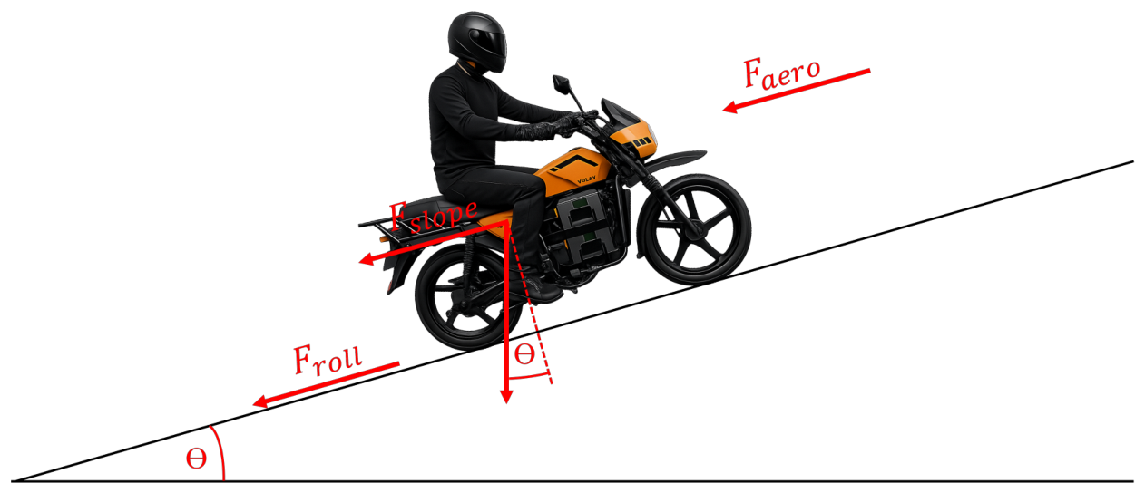
Figure 9.
Experimental setup used for the HPPC tests.
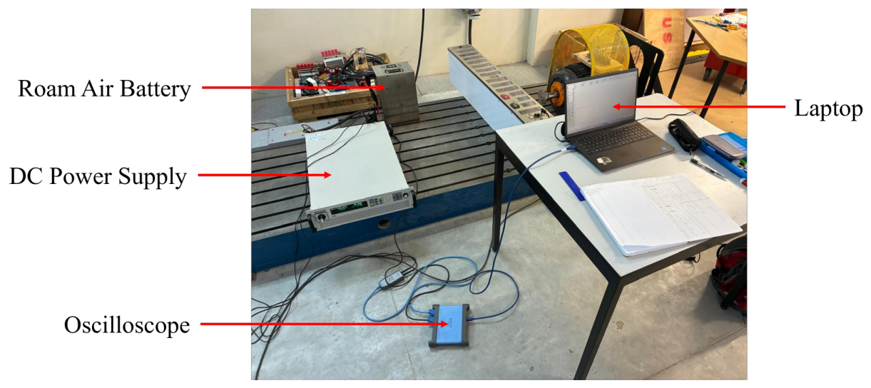
Figure 10.
Processing of the battery test data. (a) Measured OCV-SoC map of the battery pack. (b) A typical measurement file containing the terminal voltage, with markers indicating the processed sections. (c) Measured terminal voltage before and after filtering. (d) Curve fitting of the filtered terminal voltage.
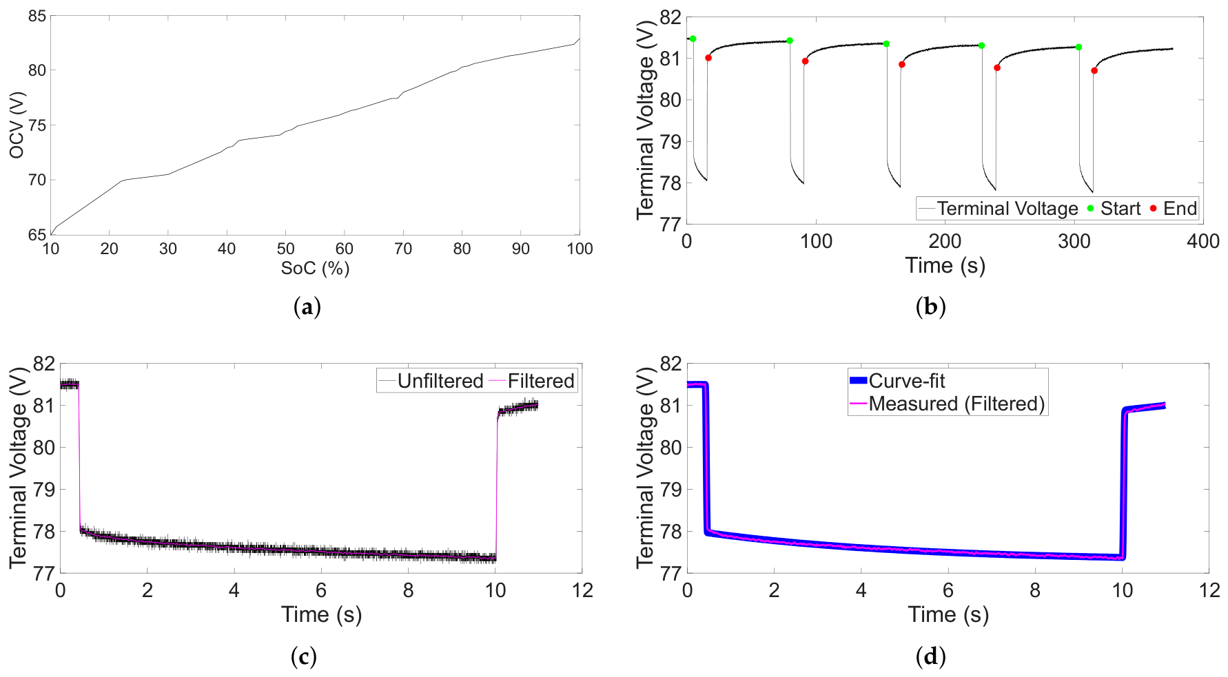
Figure 11.
ECM parameters as a function of SoC and current direction, for different current magnitudes.
Figure 11.
ECM parameters as a function of SoC and current direction, for different current magnitudes.
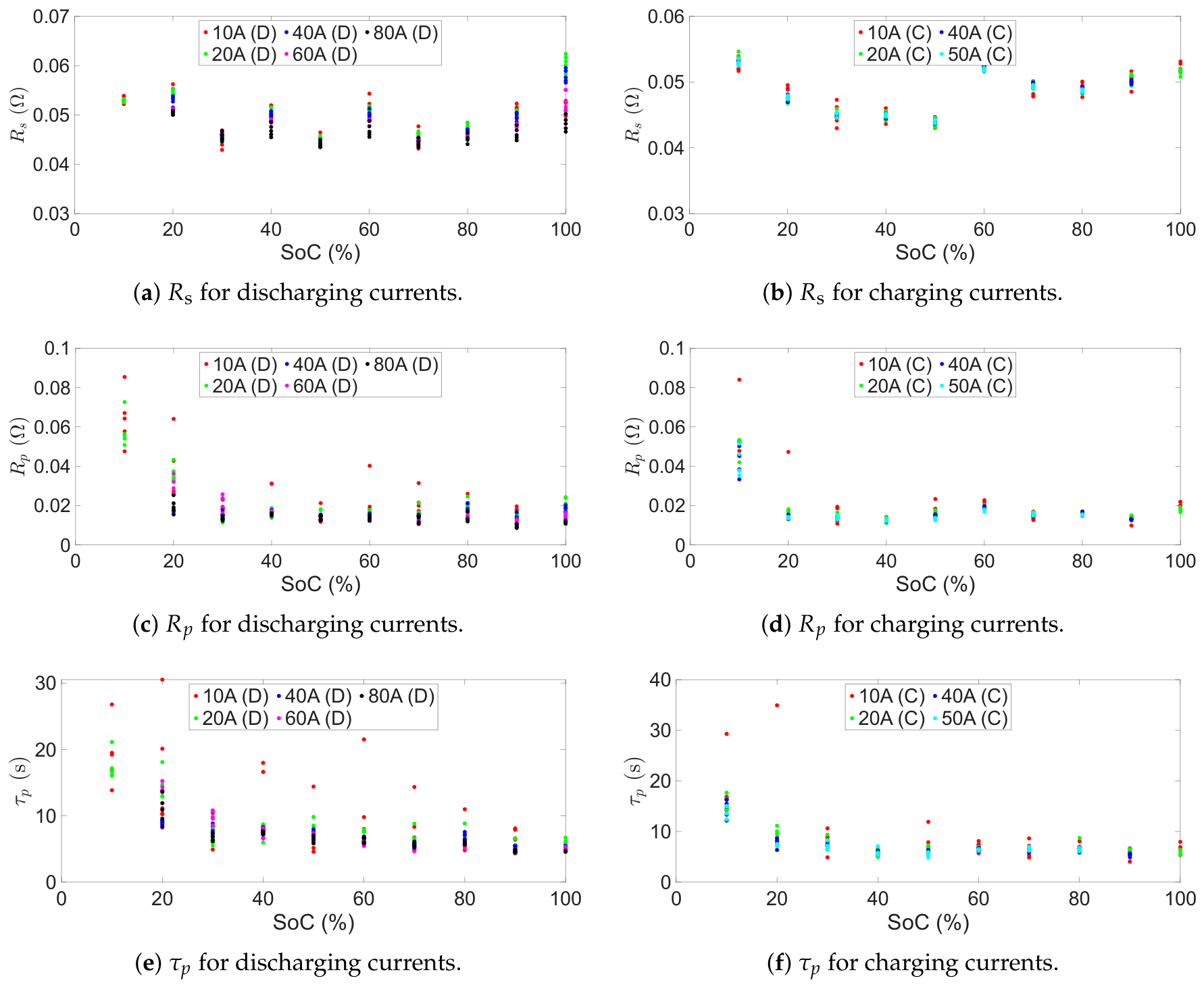
Figure 12.
ECM parameters, as a function of SoC and current direction, implemented into the battery model.
Figure 12.
ECM parameters, as a function of SoC and current direction, implemented into the battery model.
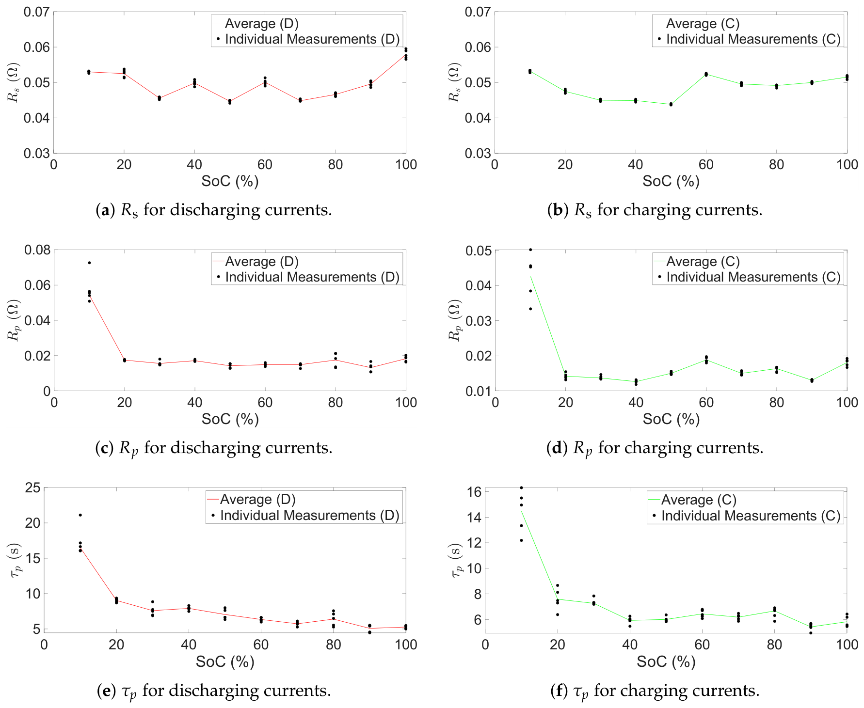
Figure 13.
Effect of speed and battery SoC on the regenerative torque. (a) Effect of speed on the regenerative torque. (b) Effect of SoC on the regenerative torque.
Figure 13.
Effect of speed and battery SoC on the regenerative torque. (a) Effect of speed on the regenerative torque. (b) Effect of SoC on the regenerative torque.
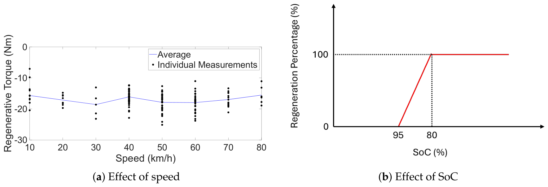
Figure 14.
Speed profiles measured from the coast-down tests. (a) One of the speed profiles measured from the unloaded drivetrain coast-down tests. (b) One of the speed profiles measured from the loaded drivetrain coast-down tests.
Figure 14.
Speed profiles measured from the coast-down tests. (a) One of the speed profiles measured from the unloaded drivetrain coast-down tests. (b) One of the speed profiles measured from the loaded drivetrain coast-down tests.
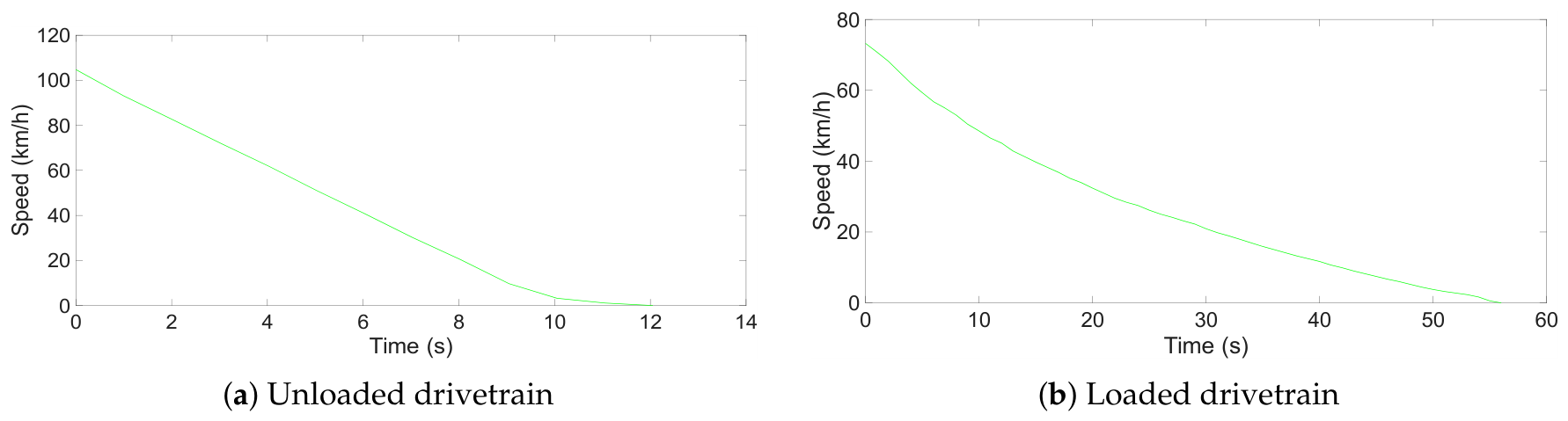
Figure 15.
Validation process of the digital twin. (a) Generation of validation data: raw telemetry data (green) and validation data (red). (b) Validation process outline.
Figure 15.
Validation process of the digital twin. (a) Generation of validation data: raw telemetry data (green) and validation data (red). (b) Validation process outline.
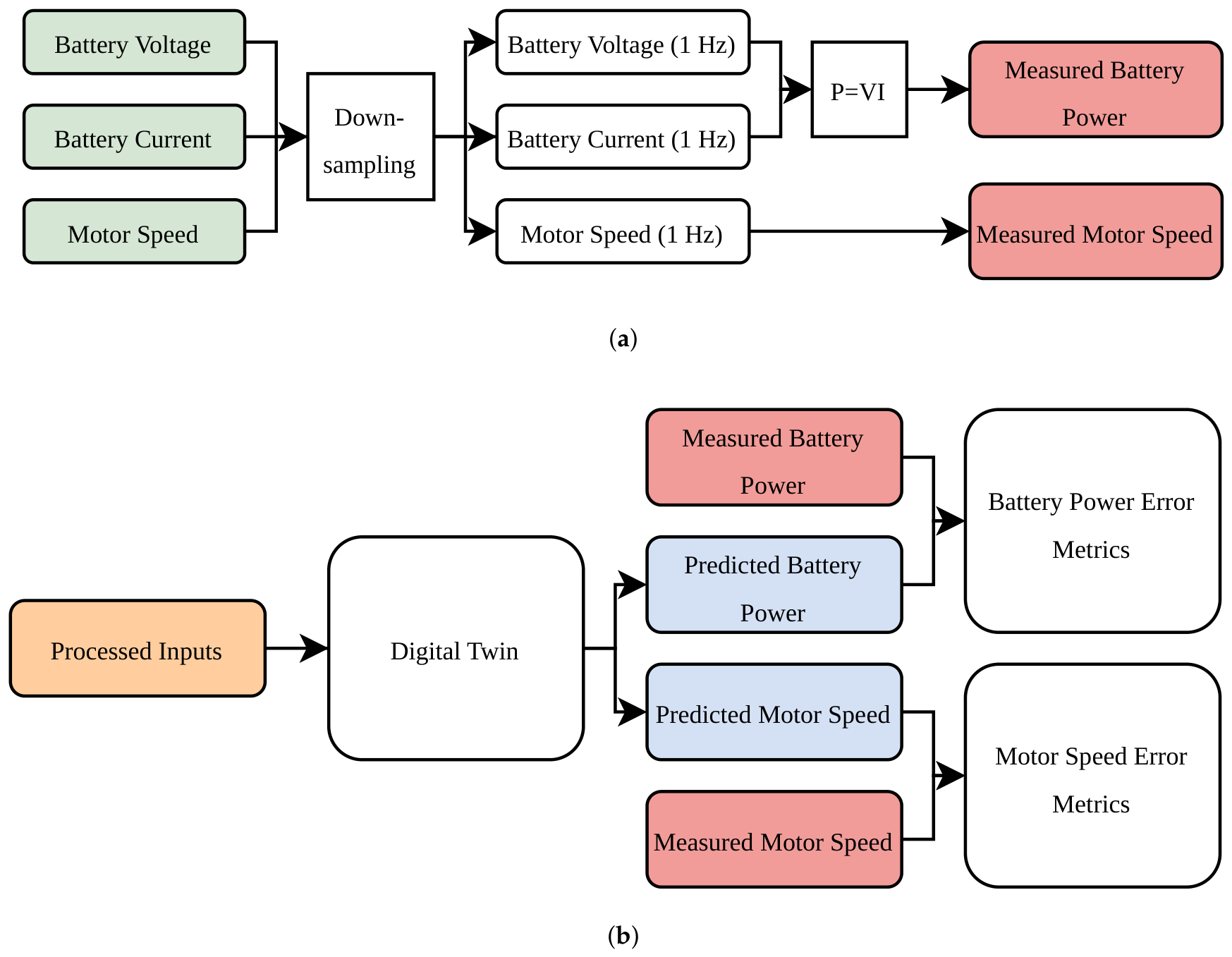
Figure 16.
Predicted terminal voltage, battery power, and motor speed of the digital twin against measured values, for six drive cycles. Trip 4 exhibits more frequent throttle modulation than the others.
Figure 16.
Predicted terminal voltage, battery power, and motor speed of the digital twin against measured values, for six drive cycles. Trip 4 exhibits more frequent throttle modulation than the others.
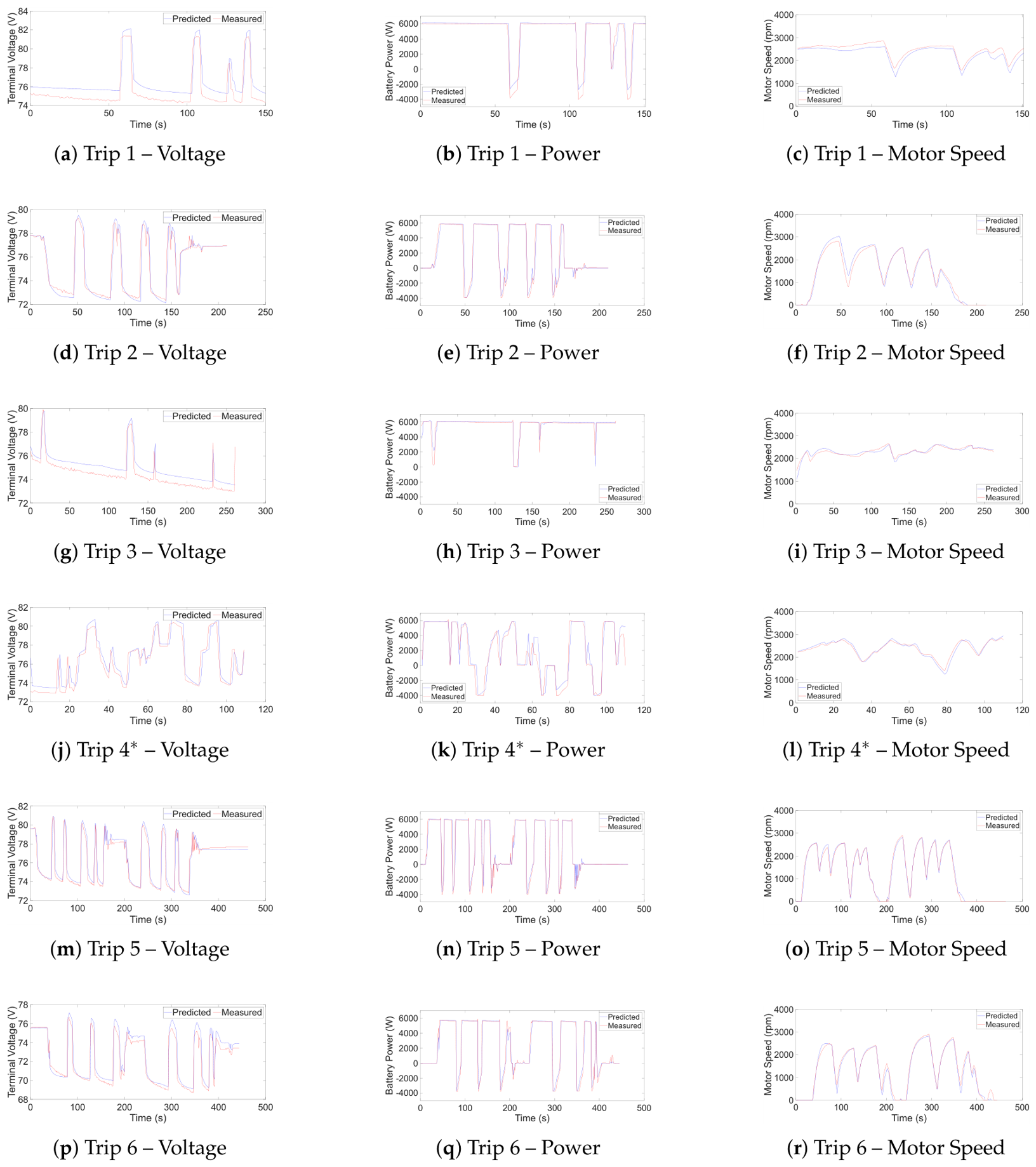

Table 1.
Parameters for Gaussian smoothing.
| Variable | Sigma (Samples) | Kernel Size (Samples) |
|---|---|---|
| Path length () | 0.75 | 5 |
| GPS altitude (h) | 1.80 | 11 |
Table 2.
Controller specifications.
| Specification | Value | Unit |
|---|---|---|
| Control type | Field-oriented control (FOC) | - |
| Control mode | Torque control | - |
| Control strategy () | Maximum torque per ampere (MTPA) | - |
| Control strategy () | Adaptive control (PI control) | - |
| Transistor type | N-channel silicon MOSFET (10N027) | - |
| Rated power | 8600 | W |
| Rated DC voltage | 72 | V |
| Rated DC current | 80 | A |
Table 3.
Parameters for the PI current controllers.
| Parameter | Value | Unit |
|---|---|---|
| Feedback current gain () | 1 | - |
| Desired lag () | 0.5 | s |
Table 4.
Parameters of the vehicle dynamics subsystem.
| Parameter | Value | Source | |
|---|---|---|---|
| Rolling resistance coefficient | 0.01 | Calculated (Section 4.4) | |
| Gross vehicle mass | m | 229.2–313.2 kg | Manufacturer (), Measured () |
| Acceleration due to gravity | g | 9.81 | - |
| Air density | 1.182–1.191 kg/ | Calculated (Ideal Gas Law) | |
| Drag coefficient | 0.61–0.68 | Calculated (Section 4.4) | |
| Frontal area | A | 0.78–0.93 | Measured (ImageJ Version 1.54t) |
| Wheel radius | 0.2953 m | Measured | |
| Sprocket ratio | 4 | Measured | |
Table 5.
Battery pack specifications.
| Specification | Value | Unit |
|---|---|---|
| Battery cell chemistry | Nickel manganese cobalt (NMC) | - |
| Nominal capacity | 45 | Ah |
| Nominal voltage | 72 | V |
| Voltage operating range | 63–84 | V |
| Maximum operating discharge current magnitude | 80 | A |
| Maximum operating charge current magnitude | 50 | A |
Table 6.
Motor specifications.
| Specification | Value | Unit |
|---|---|---|
| Motor type | IPMSM | - |
| Rated power | 6000 | W |
| Maximum torque | 54 | Nm |
| Base speed | 3800 | rpm |
| Rated voltage | 72 | V |
| Maximum phase current | 300 | |
| Interior permanent magnet synchronous motor | ||
Table 7.
Parameter values of dq motor model.
| Parameter | Value | Unit |
|---|---|---|
| Stator resistance per phase () | 3.9 | |
| D-axis stator inductance () | 0.0787 | mH |
| Q-axis stator inductance () | 0.0790 | mH |
| Permanent magnet flux linkage () | 0.02 | Wb |
Table 8.
Results summary of coast-down tests.
| Parameter | Specific Condition | Mean | Standard Deviation | Unit |
|---|---|---|---|---|
| Coulomb friction torque () | - | 2.17 | 0.049 | Nm |
| Drag coefficient () | Upright (1 person) | 0.68 | 0.14 | - |
| Low-drag (1 person) | 0.61 | 0.054 | - | |
| Upright (2 people) | 0.64 | 0.15 | - | |
| Rolling resistance coefficient () | Asphalt (1 person) | 0.01 | 0.0045 | - |
| Asphalt (2 people) | 0.013 | 0.0047 | - |
Table 9.
Description of trips.
| Trip | Description | Average Speed | Total Distance |
|---|---|---|---|
| [km/h] | [km] | ||
| 1 | Flat, high speed | 68.48 | 2.94 |
| 2 | Flat, low speed | 39.97 | 1.99 |
| 3 | Constant uphill | 64.15 | 4.75 |
| 4 | Constant downhill | 66.28 | 2.08 |
| 5 | Flat, rider only | 36.30 | 4.27 |
| 6 | Flat, rider and a passenger | 38.62 | 4.72 |
Table 10.
Digital twin results: predicted terminal voltage, battery power, and motor speed against measured values for six drive cycles.
Table 10.
Digital twin results: predicted terminal voltage, battery power, and motor speed against measured values for six drive cycles.
| Quantity | Trip | MAE | RMSE | r | |
|---|---|---|---|---|---|
| Voltage [V] | 1 | 1.1 | 1.232 | 0.174 | 0.9158 |
| 2 | 0.365 | 0.678 | 0.097 | 0.9616 | |
| 3 | 0.671 | 0.75 | 0.109 | 0.9302 | |
| 4 | 0.73 | 1.132 | 0.151 | 0.8982 | |
| 5 | 0.407 | 0.685 | 0.085 | 0.9567 | |
| 6 | 0.516 | 0.712 | 0.089 | 0.9696 | |
| Power [W] | 1 | 337 | 706 | 0.069 | 0.9705 |
| 2 | 296 | 712 | 0.071 | 0.9781 | |
| 3 | 189 | 525 | 0.085 | 0.9051 | |
| 686 | 1295 | 0.128 | 0.9349 | ||
| 5 | 267 | 700 | 0.068 | 0.9785 | |
| 6 | 292 | 666 | 0.069 | 0.9805 | |
| Motor Speed [rpm] | 1 | 158 | 176 | 0.1369 | 0.9728 |
| 2 | 117 | 167 | 0.0593 | 0.9884 | |
| 3 | 64 | 87 | 0.0727 | 0.9122 | |
| 4 | 74 | 93 | 0.0647 | 0.9770 | |
| 5 | 60 | 92 | 0.0315 | 0.9961 | |
| 6 | 93 | 134 | 0.0461 | 0.9926 | |
| a | |||||
| b The drive cycle exhibits more frequent throttle modulation than the others. | |||||
Table 11.
Energy consumption results.
| Trip | Wh/km Predicted | Wh/km Measured | Wh/km error | Wh/km error [%] | Total Energy Predicted [Wh] | Total Energy Measured [Wh] |
|---|---|---|---|---|---|---|
| 1 | 71.03 | 69.16 | 1.87 | 2.71 | 209 | 203 |
| 2 | 69.21 | 69.94 | -0.73 | -1.05 | 138 | 139 |
| 3 | 86.87 | 85.77 | 1.10 | 1.28 | 413 | 408 |
| 33.83 | 30.58 | 3.25 | 10.65 | 70 | 63 | |
| 5 | 68.50 | 67.08 | 1.42 | 2.11 | 293 | 287 |
| 6 | 64.45 | 63.53 | 0.92 | 1.45 | 304 | 300 |
| The drive cycle exhibits more frequent throttle modulation than the others. | ||||||
Disclaimer/Publisher’s Note: The statements, opinions and data contained in all publications are solely those of the individual author(s) and contributor(s) and not of MDPI and/or the editor(s). MDPI and/or the editor(s) disclaim responsibility for any injury to people or property resulting from any ideas, methods, instructions or products referred to in the content. |
© 2026 by the authors. Licensee MDPI, Basel, Switzerland. This article is an open access article distributed under the terms and conditions of the Creative Commons Attribution (CC BY) license (http://creativecommons.org/licenses/by/4.0/).
Copyright: This open access article is published under a Creative Commons CC BY 4.0 license, which permit the free download, distribution, and reuse, provided that the author and preprint are cited in any reuse.