

Submitted:
05 August 2026
Posted:
06 August 2026
You are already at the latest version
Abstract
Climate relationships with agricultural insurance claims are unlikely to be spatially uniform because crops, hazards, and insurance experience vary geographically. To identify geographic variation in climate predictors of claim severity, we fit six geographically weighted random forest models to monthly county observations from 1994 through 2022, pairing corn, soybeans, or wheat with drought or excess moisture/precipitation/rain. The outcome was logarithmically transformed positive loss per claim, adjusted to constant 2022 dollars using the Consumer Price Index for All Urban Consumers. Models included six monthly climate predictors, seasonal controls, and year, with each local forest using an adaptive neighborhood of the 10 nearest eligible counties. Total positive climate importance was greatest in the Great Plains and Midwest but varied by commodity and cause. Maximum temperature ranked first in five of the six models, while actual evapotranspiration ranked first for soybean excess moisture claims. Corn and soybean drought models emphasized maximum temperature and vapor pressure deficit, while excess moisture models showed more heterogeneous patterns. These findings demonstrate that a single national profile of climate importance cannot adequately represent local relationships between climate and claim severity. The analysis is conditional on positive payments and does not estimate claim occurrence or risk normalized for exposure.
Keywords:
crop insurance
; climate risk
; geographically weighted random forest
; spatial nonstationarity
; drought
; excess moisture
; claim severity
; permutation importance
1. Introduction
Agricultural production is exposed simultaneously to chronic climatic conditions and acute weather extremes [1]. High temperatures can reduce yields nonlinearly once crop-specific thresholds are exceeded, while water deficits, atmospheric demand, and excess precipitation can impair crop growth through distinct physiological and field-management pathways [2,3,4,5]. At broader scales, anthropogenic climate change has generally slowed agricultural productivity growth, increasing concern about how changing hazards will alter production risk and the institutions designed to manage it [6,7].
The U.S. Federal Crop Insurance Program is a central component of agricultural risk management [8]. Because indemnity records identify commodities, locations, timing, and reported causes of loss, insurance data also provide an extensive archive for examining weather-related agricultural damages [9,10]. Previous work has linked warming to increased yield risk and program costs and has shown that insurance incentives may influence adaptation to extreme heat [9,11,12,13,14]. Cause-of-loss records further show that drought and excess moisture are among the most consequential weather-related categories in the program [10,15]. These studies establish that climate matters for insured agricultural losses, but most empirical analyses estimate average relationships over large geographic domains or impose a common functional form across locations.
A spatially invariant relationship is unlikely to describe the full U.S. agricultural system. Crop calendars, cultivars, soils, irrigation, management, hazard climatology, and insurance participation vary geographically: a climate variable that is informative for claim severity in one production region may add little information elsewhere, and the locally important predictors of drought claims may differ from those associated with excess-moisture claims. National average coefficients or global machine-learning importance scores can obscure this fine-grained nonstationarity.
Geographically weighted methods address spatial nonstationarity by estimating models within locally defined subsets of the data [16]. Geographically weighted regression allows relationships between predictors and an outcome to vary across space, but it generally requires a prespecified functional form and may be difficult to interpret when relationships are nonlinear or strongly interactive [17]. Random forests provide a complementary approach by representing nonlinear relationships and interactions through ensembles of regression trees without requiring a predetermined response surface [18]. Geographically weighted random forests combine spatial localization with the flexibility of random forests by fitting separate ensembles within neighborhoods surrounding focal locations [19]. The resulting local models can be used to map geographic variation in predictor importance and model behavior. Although this approach does not provide conventional hypothesis tests or causal estimates, it is well suited to a national county panel in which the climate variables associated with agricultural insurance claim severity are expected to vary geographically.
This study asks: (1) where is the combined local usefulness of climate predictors greatest for explaining positive agricultural insurance claim severity; (2) which climate predictor is locally dominant; and, (3) how do these patterns differ among corn, soybeans, and wheat and between drought and excess-moisture damage causes? To address these questions, we analyze county–month observations from 1994–2022 using six county-centered geographically weighted random forest models, emphasizing spatial heterogeneity in conditional claim severity by evaluating the size of positive payments per claim among county–months in which at least one positive insurance payment occurred. This approach does not estimate claim probability, total expected loss, or exposure-normalized insurance risk.
2. Materials and Methods
2.1. Study Design and Analytical Units
The study domain was the conterminous United States, with insurance observations organized as a county–month–year panel for 1994–2022. Separate models were fitted for each of the six combinations formed by crossing three commodities (corn, soybeans, and wheat) with two damage causes (drought and excess moisture/precipitation/rain). Insurance records were derived from publicly available U.S. Department of Agriculture Risk Management Agency (RMA) cause-of-loss and Summary of Business resources [20,21]. Insurance payments were adjusted for inflation using the monthly U.S. city average Consumer Price Index for All Urban Consumers (CPI-U), not seasonally adjusted, and expressed in constant 2022 dollars.
The analysis was limited to county–months with at least one positive insurance payment for the specified commodity and damage cause. Observations with non-positive losses per claim were excluded because the analysis was designed to model the severity of positive insurance payments. The results therefore characterize spatial variation in climate–claim-severity relationships only for county–months in which a positive payment occurred, and do not describe the probability that a claim occurred or the overall level of agricultural insurance risk. The number of counties included in each model varies because commodity production, reported damage causes, and positive insurance payments are not distributed uniformly across the United States. The overall analytical workflow, from insurance and climate data preparation through county-centered geographically weighted random forest modeling, is summarized in Figure 1.
2.2. Claim-Severity Outcome and Inflation Adjustment
The primary response was positive real insurance loss per claim, expressed in constant 2022 U.S. dollars. Nominal losses were adjusted using the monthly Consumer Price Index for All Urban Consumers, U.S. city average, all items, not seasonally adjusted (Bureau of Labor Statistics series CUUR0000SA0) [22]. The modeled response was
where c, m, and t index county, month, and year. The logarithmic transformation reduced the leverage of the strongly right-skewed loss distribution while retaining small positive values.
Dividing loss by claim count adjusts the outcome for the number of claims represented in a county–month, but does not normalize by insured acreage, liability, premium, policy count, coverage level, or other measures of insurance exposure. The outcome therefore represents payment severity per claim, not a loss rate or total agricultural vulnerability.
2.3. Climate Predictors and Temporal Controls
Each model included six monthly climate predictors: precipitation (ppt), maximum temperature (tmax), minimum temperature (tmin), vapor-pressure deficit (vpd), actual evapotranspiration (aet), and soil moisture (soil). Together, these variables represent water supply, thermal conditions, atmospheric moisture demand, realized land-surface water use, and soil-water availability. Monthly climate and climatic water-balance data were obtained from TerraClimate through the University of Idaho’s Northwest Knowledge Network THREDDS data service [23]. The gridded data were spatially subset to the conterminous United States and aggregated to county polygons using coverage-fraction-weighted means across raster cells intersecting each county. This procedure produced one observation for each county, year, month, and climate variable. County-month climate values for 1994–2022 were then joined to the agricultural insurance records using county FIPS code, year, and month. To account for recurring seasonal structure, calendar month was represented using sine and cosine terms:
where m denotes calendar month. Calendar year was included as a continuous temporal control to absorb broad long-term changes in program structure, technology, management, reporting, and climate that were not otherwise represented by the monthly predictors.
2.4. County-Centered Geographically Weighted Random Forest
Random forests estimate an ensemble of regression trees from resampled data and randomly selected predictor subsets, allowing flexible representation of nonlinear and interacting relationships [18]. In the county-centered geographically weighted random forest design, one local random forest was centered on every eligible focal county. The focal county was represented by a reproducible anchor row used only to supply coordinates. The full monthly panel for the focal county and neighboring counties remained available to fit the local model.
Neighborhoods were defined using a location-based adaptive bandwidth. For each focal county, the primary model selected the 10 nearest unique eligible county locations, including the focal county. The bandwidth therefore referred to counties rather than panel rows. This design avoided zero-distance and duplicated-location problems that arise when repeated monthly observations are treated as independent spatial locations. Within each adaptive neighborhood, observations were weighted by distance from the focal county using a bi-square spatial kernel. These weights were supplied to the local ranger model as case weights, so observations from counties nearer the focal county contributed more strongly to fitting the local forest. Because spatial distance was defined at the county-location level, all monthly observations from the same county received the same spatial weight within a given focal model.
For observation i relative to focal county c, the spatial weight was
where is the distance between the county associated with observation i and focal county c, and is the adaptive local bandwidth. The kernel assigned its greatest weight to observations from the focal county and declined to zero at the local bandwidth.
Because each selected county contributed all eligible monthly observations, local training sample sizes varied with historical support in the focal neighborhood. Each local model used 50 trees and was fitted using the following model specification:
The principal output was county-specific permutation importance from each county-centered local random forest. Importance was calculated using the unscaled permutation measure implemented in ranger [24]. For each predictor, values were permuted among out-of-bag observations, and importance was quantified as the average increase in out-of-bag squared prediction error relative to the unpermuted predictions. Larger positive values indicate greater predictive reliance on a variable within the fitted local model, while values near zero indicate little contribution to out-of-bag predictive performance. Negative values can occur when permutation does not degrade, or slightly improves, predictive performance, and should not be interpreted as evidence of a protective effect. Permutation importance measures predictive reliance rather than effect direction; it thus does not indicate whether higher predictor values increase or decrease claim severity and should not be interpreted causally.
A second run using an adaptive bandwidth of 25 unique county locations was generated as a sensitivity analysis. While the run is the primary analysis because it preserves greater geographic localization, the results were used to compare with the primary models using county-level correlations in total positive climate importance, dominant predictor agreement, model-wide predictor-rank correlations, and adjacent-county roughness.
2.5. Climate Importance Metrics and Map Construction
One direct county-level model output and two derived county-level summaries were used. The direct output was the signed permutation importance, , for climate predictor j at focal county c. Variable-specific maps display these values, including positive, near-zero, and negative importance values.
The first derived summary was total positive climate importance for focal county c:
where contains the six climate predictors. This index summarizes their combined positive importance without allowing negative values to offset positive values.
The second derived summary was the dominant local climate predictor,
provided that at least one climate predictor had positive importance. Counties with no positive climate importance were assigned a separate category. Dominance identifies the predictor with the largest positive importance within a county; it does not imply that its importance differs significantly from that of the second ranked predictor. Model-wide means and medians were calculated across eligible focal counties. Because importance scales depend on the fitted response and local data structure, comparisons of raw importance magnitudes across separately fitted models are purely descriptive. Within-model rankings and mapped spatial variation therefore provide the primary evidence.
Panel construction, spatial processing, GWRF estimation, summary statistics, and figure production were implemented in R 4.5.2. Local random forests were fitted using version 0.1.0 of the gwrf package [25], which was developed by the author to support geographically weighted random forests with adaptive neighborhoods defined by unique spatial locations. The package uses ranger (version 0.18.1) as the random forest engine [24]. This implementation allowed repeated county-month observations to be included without treating repeated rows from the same county as distinct neighboring locations. Core data management, spatial processing, and visualization packages included arrow, dplyr, sf, terra, and ggplot2. Analysis code, package-version information, and supporting metadata are provided in the Data Availability Statement.
3. Results
3.1. Panel Coverage and Local Training Support
The six models included 74,527–129,966 eligible county–month–year observations accumulated over the full 1994–2022 study period, representing 1,722–1,934 unique focal counties (Table 1). Each observation corresponded to one county in one month and year for a specified commodity and damage cause, conditional on a positive insurance payment. Corn and soybean observations were concentrated across the central and eastern United States, whereas wheat had a broader western and northern footprint. Mean local training support, defined as the number of eligible panel observations available to an individual county-centered forest from its adaptive county neighborhood, ranged from 426.4 to 759.1 observations across models. Although average local support was substantially larger, a small number of peripheral focal counties had limited training data, with the minimum local neighborhood containing 14 panel observations. These differences reflect commodity production geography and the frequency of eligible positive-payment observations.
Figure 2 summarizes the analytical workflow. For each focal county, the adaptive neighborhood was defined using unique county locations, while all eligible monthly observations from the selected counties were retained for local model fitting. The focal anchor observation supplied the coordinates used to center the local model and was not interpreted as a county-average prediction or residual.
3.2. Model-Wide Climate-Importance Rankings
Permutation importance values represent unscaled increases in out-of-bag squared prediction error and are therefore not restricted to values between zero and one; larger positive values indicate greater predictive reliance within a fitted model. When averaged across focal counties, maximum temperature had the highest mean permutation importance in five of the six models (Table 2). Its prominence was greatest in the corn and soybean drought models, with mean importance values of 0.765 and 0.793, respectively. In these two models, vapor pressure deficit ranked second (0.712 for corn and 0.617 for soybeans), followed by minimum temperature. The only exception to the overall maximum-temperature ranking was soybean excess moisture, with actual evapotranspiration ranked first (0.517), followed by maximum and minimum temperature. Corn excess moisture likewise showed relatively little separation among maximum temperature, actual evapotranspiration, and minimum temperature. The wheat models had lower mean climate-importance values overall and less differentiation among the leading thermal and atmospheric-demand predictors.
Year had the highest mean permutation importance among the temporal controls in all six models. Mean year importance ranged from 0.780 for wheat excess moisture to 2.284 for soybean excess moisture, with particularly high values in the corn- and soybean-excess-moisture models. This pattern indicates that broad temporal structure contributed substantially to local prediction. Because the year term may capture a mixture of technological change, policy and reporting shifts, changes in exposure and coverage, and long-term climatic variation, it was treated as a control variable rather than as a climate predictor.
3.3. Total Positive Climate Importance
Total positive climate importance (the sum of positive local permutation-importance values across the six climate predictors) varied substantially among counties in every model (Figure 3). In the corn and soybean models, counties with the highest values of this measure were concentrated primarily across the central and northern Great Plains and the western Corn Belt, especially in parts of the Dakotas, Nebraska, Kansas, Iowa, and Minnesota. This pattern was most spatially continuous in the corn-drought and soybean-drought models. The corresponding excess-moisture models retained a central Great Plains and Midwest concentration but displayed more localized hotspots and less continuous extensions into eastern and southern portions of their model domains.
Wheat displayed a different geographic pattern. In the drought model, elevated total positive climate importance extended farther west through portions of the northern Plains, southern High Plains, and interior West, while values were generally lower across many central-eastern counties. The wheat excess-moisture model showed elevated values across parts of the northern tier and central-to-southern Plains, together with scattered hotspots elsewhere. Collectively, the six maps demonstrate that total positive climate importance varied spatially rather than forming a geographically uniform pattern.
3.4. Dominant Local Climate Predictors
The identity of the climate predictor with the greatest positive local permutation importance varied across space, although several coherent regional patterns were evident (Figure 4). Maximum temperature was the dominant predictor across broad portions of the corn- and soybean-drought domains, particularly from the central Great Plains through much of the Midwest. Vapor pressure deficit and other climate variables were dominant along portions of the western and northern margins of these domains and in smaller local clusters. In the corn- and soybean-excess-moisture models, actual evapotranspiration was dominant across a broad Midwestern corridor extending approximately from Nebraska through Iowa, Illinois, Indiana, and Ohio. Outside this corridor, the excess-moisture maps showed greater local variation among maximum temperature, minimum temperature, precipitation, soil moisture, vapor pressure deficit, and actual evapotranspiration.
The wheat-drought model displayed a different and more fragmented geographic pattern. Vapor pressure deficit was dominant across much of the northern portion of the wheat domain, particularly through parts of the northern Great Plains, whereas minimum temperature was prominent in the southern High Plains, including the Texas Panhandle and adjacent areas. Elsewhere, the dominant predictor changed frequently among neighboring counties, and some counties had no positive permutation importance for any of the six climate predictors. The wheat excess-moisture model was the most geographically heterogeneous, with frequent local changes in the highest-ranked predictor and no single climate variable dominating across a broad region.
These categorical maps represent the predictor with the highest positive permutation importance within each county. They should therefore be interpreted as local rankings rather than evidence that the mapped predictor controlled claim severity or was the sole driver of losses. Where two or more predictors had similar importance values, relatively small differences could determine the mapped category.
3.5. Spatial Variation in Maximum Temperature Importance
Because maximum temperature had the highest mean permutation importance in five of the six models, its county-level importance was examined in greater detail as a representative variable-specific result, with Figure 5 illustrating why model-wide rankings alone are incomplete. In the corn- and soybean-drought models, maximum temperature showed broadly positive importance across the Great Plains, Midwest, and parts of the eastern production domains, with localized areas of particularly high importance embedded within these regions. The corresponding excess-moisture models also showed positive maximum-temperature importance across much of the central agricultural region, but the spatial pattern was weaker and more variable, with scattered near-zero and negative values.
In the wheat-drought model, positive maximum-temperature importance extended across portions of the northern Plains, southern High Plains, and interior West. The wheat excess-moisture model showed a weaker and more discontinuous spatial pattern, although localized areas of elevated importance remained. Positive values indicate that permuting maximum-temperature values increased out-of-bag prediction error and therefore reduced local predictive performance. They do not demonstrate that higher temperatures caused larger insurance payments. Determining effect direction and response shape would require a separate model-interpretation analysis beyond the scope of this study.
3.6. Bandwidth Sensitivity
The broader adaptive neighborhood of unique county locations produced results that were generally consistent with the primary analysis, although the exact identity of the dominant local predictor was more sensitive to bandwidth choice (Table 3). Across the six commodity–damage-cause models, Pearson correlations in county-level total positive climate importance between the two bandwidths ranged from 0.792 to 0.895, and Spearman rank correlations ranged from 0.750 to 0.897. Model-wide correlations in the rankings of the six climate predictors ranged from 0.943 to 1.000, and the top-ranked predictor was unchanged in five of the six models.
The only change in the top-ranked model-wide predictor occurred in the wheat-drought model, for which maximum and minimum temperature were nearly indistinguishable under the primary bandwidth. Maximum temperature ranked first under , with a mean permutation importance of 0.366939, compared with 0.366867 for minimum temperature. Under , minimum temperature ranked slightly above maximum temperature. This change therefore reflected a near-tie rather than a substantial reordering of predictor importance.
County-level agreement in the dominant climate predictor ranged from 34.8% to 61.7%, indicating that the precise categorical assignment of the highest-ranked predictor was more bandwidth sensitive than total climate importance or model-wide predictor rankings. The broader neighborhoods substantially increased local training support and reduced standardized adjacent-county roughness by 15.6% to 27.4% across the six models. Thus, the broader bandwidth produced smoother importance surfaces and altered some local predictor classifications, but it did not materially change the broader conclusions concerning geographic variation in climate importance and model-wide predictor rankings.
4. Discussion
4.1. Climate-Claim Relationships Are Spatially Nonstationary
The central finding is that the climate information associated with positive agricultural insurance claim severity varies geographically. Both total positive climate importance and the identity of the highest-ranked climate predictor differed among counties, even within the same commodity and reported damage cause. Model-wide rankings therefore summarize broad tendencies but do not fully describe local climate–claim relationships.
The bandwidth sensitivity analysis supports this interpretation (Table 3). County-level total positive climate importance remained strongly correlated between the and models, and model-wide predictor rankings were nearly unchanged. In contrast, agreement in the identity of the dominant local predictor was lower, and the broader neighborhoods produced smoother spatial surfaces. Broad geographic patterns were therefore more robust than the precise county-level classification of the highest-ranked predictor. The dominant-predictor maps should be interpreted as spatially varying local rankings rather than as fixed boundaries between mechanistically distinct regions.
This result is consistent with the rationale for geographically weighted modeling. Observations assigned the same national outcome category may arise from different local combinations of hazard exposure, cropping systems, soils, water availability, management, and insurance structure. Geographical random forests make this heterogeneity explicit by fitting a separate nonlinear ensemble around each focal location [19]. In this study, the method does not simply identify where insurance payments were large. It identifies where climate variables contributed more or less to locally predicting the severity of positive payments that had already occurred.
4.2. Drought Claims Emphasize Heat and Atmospheric Demand
Maximum temperature and vapor pressure deficit were the two highest mean-ranked climate variables in both corn and soybean drought models. Their maps also showed broad areas of positive importance across the central production belt. This pattern is physically plausible because high temperature and atmospheric moisture demand can intensify crop water stress and amplify the effects of precipitation deficits [26,27,28,29]. Previous yield and insurance studies have documented nonlinear heat damages, increased yield risk under warming, and potential insurance-related disincentives to adaptation to extreme heat [2,11,13]. The GWRF results extend that literature by showing that predictive usefulness varies considerably within the national crop domain.
The analysis does not determine whether temperature or vapor pressure deficit is the proximate cause of higher payment severity, nor can correlated climate predictors be interpreted independently. Maximum temperature, minimum temperature, vapor pressure deficit, evapotranspiration, and soil moisture are physically linked. Permutation may distribute predictive credit among correlated variables differently across local forests [30,31]. The appropriate inference is that positive drought-claim severity contains a strong and geographically variable hydrothermal signal, not that any single climate variable has an isolated causal effect.
4.3. Excess Moisture Claims Reflect Multiple Hydroclimatic Pathways
The excess-moisture models produced more heterogeneous dominant-predictor mosaics than the corn and soybean drought models. Actual evapotranspiration ranked first for soybean excess moisture and nearly tied with maximum temperature for corn excess moisture. Precipitation itself was not the highest mean-ranked variable in either model. This does not imply that precipitation was unimportant to excess-moisture claims. Monthly precipitation totals may incompletely represent saturation, drainage, antecedent soil conditions, evapotranspirative demand, field access, crop stage, and submonthly precipitation intensity. Excess precipitation can damage crops through delayed planting, waterlogging, erosion, disease, and reduced field operations [3,32,33,34].
The local importance of actual evapotranspiration, soil moisture, and temperature may reflect the broader water balance and crop-development context in which precipitation occurs rather than independent causal effects. Future directional analyses should examine interactions and conditional response shapes rather than interpreting importance maps as additive effects. Event-scale precipitation intensity and antecedent wetness metrics may improve the representation of excess moisture processes.
4.4. Wheat Differs from Corn and Soybeans
Wheat models had lower mean climate-importance values and a different geographic footprint. Wheat production spans winter and spring systems, dryland and irrigated regions, and a wider range of western and northern climates than the primary corn and soybean domains. These differences likely contribute to the more fragmented dominant-predictor maps and counties with no positive climate importance in the wheat drought model.
Lower mean importance does not imply that wheat claim severity is insensitive to climate. It indicates that, given the monthly predictors, temporal controls, local sample sizes, and response definition, permuting individual climate variables caused a smaller average degradation in local predictive performance. Lower support in some wheat neighborhoods and greater production-system heterogeneity may also reduce stability. The local-support maps retained in the supplement are therefore important when interpreting geographically isolated patterns.
4.5. Long-Term Temporal Structure
The models retained substantial long-term temporal structure beyond that represented by the monthly climate predictors and seasonal controls. The continuous calendar-year covariate had the highest mean permutation importance of all predictors in every model, particularly in the corn- and soybean-excess-moisture models. However, calendar year is not a mechanistic driver: it may be absorbing changes in commodity prices and insurance coverage, technology, yields and management, program and reporting practices, the geographic composition of insured production, and long-term climate. Insurance subsidies may also influence crop choices and therefore the composition and geographic distribution of insured production [35].
Including calendar year reduces the likelihood that the climate predictors serve as proxies for all long-term change, but it does not identify the source of the remaining temporal variation. Because the covariate may represent multiple climatic and nonclimatic processes simultaneously, its importance should not be interpreted as evidence of any single temporal mechanism. Future work could compare defined multi-year periods or fit time-varying local models. Such work should be treated as a separate temporal-change analysis rather than inferred from the full-period atlas.
4.6. Implications for Agricultural Risk Analysis
The findings have three methodological implications. First, national agricultural-risk models should evaluate spatial nonstationarity explicitly rather than assume that a single climate-response structure applies across all production regions. Second, the most predictively useful climate variables may differ by commodity, reported damage cause, and location, suggesting that predictor selection and model interpretation should account for regional production and hazard contexts. Third, risk communication should distinguish among claim occurrence, conditional claim severity, and exposure-adjusted loss rates because these outcomes answer different scientific and actuarial questions.
The maps provide a geographic screening framework for identifying regions where more detailed process-based or actuarial analysis may be warranted. However, they are not premium-rating maps and should not be used directly to recommend insurance prices or program changes. Such applications would require explicit information on liability, insured acreage, coverage, and other measures of exposure, together with actuarial validation, decision-specific out-of-sample testing, and careful consideration of policy and producer behavior. Previous studies have shown that climate change can affect both yield risk and Federal Crop Insurance Program costs [6,12,13,14]. The present results suggest that these effects may be geographically differentiated in ways that pooled national models can obscure.
4.7. Limitations
Several aspects of the data and modeling approach limit how these results should be interpreted. The analysis is conditional on county- months with at least one positive insurance payment; the models therefore do not estimate whether a claim occurs, and cannot be interpreted as models of unconditional expected loss. Although dividing total payments by claim count adjusts the outcome for the number of claims, it does not control for insured acreage, liability, policy characteristics, coverage levels, price elections, or participation. Spatial differences may thus reflect both physical loss processes and the composition of the insurance system.
Reported damage cause is an administrative classification: a claim recorded as drought or excess moisture may involve interacting hazards, and classification or reporting practices may vary over time and space. Monthly county-level climate summaries may also obscure short-duration extremes, within-county environmental variation, crop stage timing, irrigation, soil properties, and antecedent conditions. In addition, local permutation importance is sensitive to predictor correlation, local training support, and model specification [30,31]. It measures predictive usefulness but does not provide effect direction, statistical significance, or causal attribution.
Some county-centered neighborhoods had relatively small local training samples, particularly in the wheat models, because adaptive neighborhoods guarantee a specified number of county locations rather than a fixed number of county–month observations. Finally, the bandwidth sensitivity analysis indicated that broad geographic patterns and model-wide predictor rankings were generally stable, but the exact county-level classification of the dominant climate predictor remained sensitive to neighborhood size.
5. Conclusions
County-centered geographically weighted random forests revealed substantial spatial heterogeneity in the climate predictors associated with positive agricultural insurance claim severity across the conterminous United States. Maximum temperature was the highest mean-ranked climate predictor in five of the six commodity–damage-cause models, while actual evapotranspiration ranked first for soybean excess-moisture claims. Maximum temperature and vapor pressure deficit were particularly prominent in the corn- and soybean-drought models, whereas the excess-moisture models exhibited more heterogeneous local combinations of temperature, evapotranspiration, precipitation, soil moisture, and atmospheric moisture demand. The wheat models had a broader geographic footprint, lower mean climate-importance values, and more fragmented local predictor patterns than the corn and soybean models.
The analysis also demonstrated that broad model-wide rankings do not fully represent local climate–claim relationships. Total positive climate importance and the identity of the highest-ranked climate predictor varied among counties within the same commodity and reported damage cause. The bandwidth sensitivity analysis showed that broad geographic patterns and model-wide predictor rankings were generally consistent between the and neighborhoods, although the precise county-level classification of the dominant predictor was more sensitive to neighborhood size. These results support the use of spatially localized models while also emphasizing that mapped predictor boundaries should not be interpreted as fixed or mechanistically distinct regions.
The findings apply specifically to payment severity among county–months with at least one positive insurance payment. They do not estimate claim probability, unconditional expected loss, exposure-adjusted risk, or causal climate effects. Nevertheless, the atlas provides a reproducible geographic screening framework for identifying where climate variables contribute differently to the local prediction of positive claim severity. Agricultural risk analyses should therefore evaluate spatial nonstationarity explicitly and distinguish among claim occurrence, conditional claim severity, and exposure-adjusted loss. Future research should integrate insured acreage, liability, coverage, and other measures of exposure; evaluate directional and interactive climate effects; examine temporal change; and investigate the local processes underlying the geographic patterns identified here.
Supplementary Materials
The following supporting information can be downloaded at website of this paper posted on Preprints.org, The supporting information includes the complete county-centered GWRF analysis for all six commodity–damage-cause models, with historical panel support, local training support, total positive climate importance, dominant climate predictor, and variable-specific importance maps.
Author Contributions
E.S. was solely responsible for all aspects of the study, including conceptualization, methodology, software, validation, formal analysis, investigation, data curation, visualization, project administration, and preparation and revision of the manuscript. The author has read and agreed to the published version of the manuscript.
Funding
This research was supported by faculty startup funds provided by Baylor University’s College of Arts and Sciences and the School of Earth and Environmental Sciences.
Institutional Review Board Statement
Not applicable. This study used publicly available aggregate administrative and environmental data and did not involve human participants or animals.
Informed Consent Statement
Not applicable.
Data Availability Statement
The original agricultural insurance data used in this study are publicly available from the U.S. Department of Agriculture Risk Management Agency. Cause of Loss data are available at https://www.rma.usda.gov/tools-reports/summary-of-business/cause-loss, and Summary of Business data are available at https://www.rma.usda.gov/tools-reports/summary-of-business. Monthly climate and climatic water-balance data are publicly available from TerraClimate at https://www.climatologylab.org/terraclimate.html. Monthly Consumer Price Index data for series CUUR0000SA0 are publicly available from the U.S. Bureau of Labor Statistics at https://data.bls.gov/timeseries/CUUR0000SA0. The processed analytical datasets, model outputs, supporting metadata, and code required to reproduce the analyses and figures are archived in Dryad (https://datadryad.org) at https://doi.org/10.5061/dryad.r4xgxd2vm. The gwrf R package is available at https://github.com/hac-lab/gwrf.
Conflicts of Interest
The author declares no conflicts of interest.
Acknowledgments
The author gratefully acknowledges the institutional support provided by Baylor University’s College of Arts & Sciences, particularly through the School of Earth and Environmental Sciences.
Abbreviations
The following abbreviations are used in this manuscript:
| CPI-U | Consumer Price Index for All Urban Consumers |
| GWRF | Geographically weighted random forest |
| RMA | Risk Management Agency |
| USDA | U.S. Department of Agriculture |
| THREDDS | Thematic Real-time Environmental Distributed Data Services |
References
- Lesk, C.; Rowhani, P.; Ramankutty, N. Influence of extreme weather disasters on global crop production. Nature 2016, 529, 84–87. [Google Scholar] [CrossRef] [PubMed]
- Schlenker, W.; Roberts, M.J. Nonlinear temperature effects indicate severe damages to U.S. crop yields under climate change. Proc. Natl. Acad. Sci. USA 2009, 106, 15594–15598. [Google Scholar] [CrossRef] [PubMed]
- Rosenzweig, C.; Tubiello, F.N.; Goldberg, R.; Mills, E.; Bloomfield, J. Increased crop damage in the US from excess precipitation under climate change. Glob. Environ. Change 2002, 12, 197–202. [Google Scholar] [CrossRef]
- Schauberger, B.; Archontoulis, S.; Arneth, A.; Balkovic, J.; Ciais, P.; Deryng, D.; Elliott, J.; Folberth, C.; Khabarov, N.; Müller, C.; et al. Consistent negative response of US crops to high temperatures in observations and crop models. Nat. Commun. 2017, 8, 13931. [Google Scholar] [CrossRef] [PubMed]
- Zhao, C.; Liu, B.; Piao, S.; Wang, X.; Lobell, D.B.; Huang, Y.; Huang, M.; Yao, Y.; Bassu, S.; Ciais, P.; et al. Temperature increase reduces global yields of major crops in four independent estimates. Proc. Natl. Acad. Sci. U.S.A. 2017, 114, 9326–9331. [Google Scholar] [CrossRef] [PubMed]
- Lobell, D.B.; Schlenker, W.; Costa-Roberts, J. Climate trends and global crop production since 1980. Science 2011, 333, 616–620. [Google Scholar] [CrossRef] [PubMed]
- Ortiz-Bobea, A.; Ault, T.R.; Carrillo, C.M.; Chambers, R.G.; Lobell, D.B. Anthropogenic climate change has slowed global agricultural productivity growth. Nat. Clim. Chang. 2021, 11, 306–312. [Google Scholar] [CrossRef]
- Miranda, M.J.; Glauber, J.W. Systemic Risk, Reinsurance, and the Failure of Crop Insurance Markets. Am. J. Agric. Econ. 1997, 79, 206–215. [Google Scholar] [CrossRef]
- Seamon, E.; Gessler, P.E.; Abatzoglou, J.T.; Mote, P.W.; Lee, S.S. A climatic random forest model of agricultural insurance loss for the Northwest United States. Environ. Data Sci. 2022, 1, 1–9. [Google Scholar] [CrossRef]
- Seamon, E.; Gessler, P.E.; Abatzoglou, J.T.; Mote, P.W.; Lee, S.S. Climatic Damage Cause Variations of Agricultural Insurance Loss for the Pacific Northwest Region of the United States. Agriculture 2023, 13, 2214. [Google Scholar] [CrossRef]
- Annan, F.; Schlenker, W. Federal Crop Insurance and the Disincentive to Adapt to Extreme Heat. Am. Econ. Rev. 2015, 105, 262–266. [Google Scholar] [CrossRef]
- Tack, J.; Coble, K.; Barnett, B. Warming temperatures will likely induce higher premium rates and government outlays for the U.S. crop insurance program. Agric. Econ. 2018, 49, 635–647. [Google Scholar] [CrossRef]
- Perry, E.D.; Yu, J.; Tack, J. Using insurance data to quantify the multidimensional impacts of warming temperatures on yield risk. Nat. Commun. 2020, 11, 4542. [Google Scholar] [CrossRef] [PubMed]
- Crane-Droesch, A.; Marshall, E.; Rosch, S.; Riddle, A.; Cooper, J.; Wallander, S. Climate Change and Agricultural Risk Management Into the 21st Century. Economic Research Report Number 266. 2019. [Google Scholar] [CrossRef]
- Reyes, J.J.; Elias, E. Spatio-temporal variation of crop loss in the United States from 2001 to 2016. Environ. Res. Lett. 2019, 14, 074017. [Google Scholar] [CrossRef]
- Brunsdon, C.; Fotheringham, A.S.; Charlton, M.E. Geographically Weighted Regression: A Method for Exploring Spatial Nonstationarity. Geogr. Anal. 1996, 28, 281–298. [Google Scholar] [CrossRef]
- Fotheringham, A.S.; Yang, W.; Kang, W. Multiscale Geographically Weighted Regression (MGWR). Ann. Am. Assoc. Geogr. 2017, 107, 1247–1265. [Google Scholar] [CrossRef]
- Breiman, L. Random Forests. Mach. Learn. 2001, 45, 5–32. [Google Scholar] [CrossRef]
- Georganos, S.; Grippa, T.; Niang Gadiaga, A.; Linard, C.; Lennert, M.; Vanhuysse, S.; Mboga, N.; Wolff, E.; Kalogirou, S. Geographical random forests: a spatial extension of the random forest algorithm to address spatial heterogeneity in remote sensing and population modelling. Geocarto Int. 2021, 36, 121–136. [Google Scholar] [CrossRef]
- U.S. Department of Agriculture, Risk Management Agency. Cause of Loss Historical Data Files.
- U.S. Department of Agriculture; Risk Management Agency. Summary of Business Historical Data Files.
- U.S. Bureau of Labor Statistics. Bureau of Labor Statistics Consumer Price Index (CPI-U). [CrossRef]
- Abatzoglou, J.T.; Dobrowski, S.Z.; Parks, S.A.; Hegewisch, K.C. TerraClimate, a high-resolution global dataset of monthly climate and climatic water balance from 1958-2015. Sci. Data 2018, 5, 1–12. [Google Scholar] [CrossRef] [PubMed]
- Wright, M.N.; Ziegler, A. ranger: A Fast Implementation of Random Forests for High Dimensional Data in C++ and R. Soft 2017, 77. [Google Scholar] [CrossRef]
- Seamon, E. gwrf: Geographically Weighted Random Forests, 2026. Status: Submitted to the Comprehensive R Archive Network.
- Lobell, D.B.; Hammer, G.L.; McLean, G.; Messina, C.; Roberts, M.J.; Schlenker, W. The critical role of extreme heat for maize production in the United States. Nat. Clim. Change 2013, 3, 497–501. [Google Scholar] [CrossRef]
- Grossiord, C.; Buckley, T.N.; Cernusak, L.A.; Novick, K.A.; Poulter, B.; Siegwolf, R.T.W.; Sperry, J.S.; McDowell, N.G. Plant responses to rising vapor pressure deficit. New Phytol. 2020, 226, 1550–1566. [Google Scholar] [CrossRef] [PubMed]
- Novick, K.A.; Ficklin, D.L.; Stoy, P.C.; Williams, C.A.; Bohrer, G.; Oishi, A.; Papuga, S.A.; Blanken, P.D.; Noormets, A.; Sulman, B.N.; et al. The increasing importance of atmospheric demand for ecosystem water and carbon fluxes. Nat. Clim. Change 2016, 6, 1023–1027. [Google Scholar] [CrossRef]
- Lesk, C.; Anderson, W.; Rigden, A.; Coast, O.; Jägermeyr, J.; McDermid, S.; Davis, K.F.; Konar, M. Compound heat and moisture extreme impacts on global crop yields under climate change. Nat. Rev. Earth Env. 2022, 3, 872–889. [Google Scholar] [CrossRef]
- Strobl, C.; Boulesteix, A.L.; Kneib, T.; Augustin, T.; Zeileis, A. Conditional variable importance for random forests. BMC Bioinform. 2008, 9, 307. [Google Scholar] [CrossRef] [PubMed]
- Nicodemus, K.K.; Malley, J.D.; Strobl, C.; Ziegler, A. The behaviour of random forest permutation-based variable importance measures under predictor correlation. BMC Bioinform. 2010, 11, 110. [Google Scholar] [CrossRef] [PubMed]
- Tian, L.x.; Zhang, Y.c.; Chen, P.l.; Zhang, F.f.; Li, J.; Yan, F.; Dong, Y.; Feng, B.l. How Does the Waterlogging Regime Affect Crop Yield? A Global Meta-Analysis. Front. Plant Sci. 2021, 12, 634898. [Google Scholar] [CrossRef] [PubMed]
- Voesenek, L.A.C.J.; Bailey-Serres, J. Flood adaptive traits and processes: an overview. New Phytol. 2015, 206, 57–73. [Google Scholar] [CrossRef] [PubMed]
- Setter, T.L.; Waters, I.; Sharma, S.K.; Singh, K.N.; Kulshreshtha, N.; Yaduvanshi, N.P.S.; Ram, P.C.; Singh, B.N.; Rane, J.; McDonald, G.; et al. Review of wheat improvement for waterlogging tolerance in Australia and India: the importance of anaerobiosis and element toxicities associated with different soils. Ann. Bot. 2009, 103, 221–235. [Google Scholar] [CrossRef] [PubMed]
- Yu, J.; Sumner, D.A. Effects of subsidized crop insurance on crop choices. Agric. Econ. (United Kingdom) 2018, 49, 533–545. [Google Scholar] [CrossRef]
Figure 1.
Analytical workflow for evaluating spatial heterogeneity in climate–agricultural insurance claim severity. County-month insurance records were combined with monthly climate data, and indemnity payments were adjusted to constant 2022 dollars using monthly CPI-U. Separate datasets were constructed for six commodity × damage-cause combinations. For each eligible focal county, a geographically weighted random forest was fit using the complete monthly panel from the focal county and its adaptive neighborhood of the 10 nearest unique county locations. Permutation importance represents local predictive usefulness and does not indicate effect direction or causality.
Figure 1.
Analytical workflow for evaluating spatial heterogeneity in climate–agricultural insurance claim severity. County-month insurance records were combined with monthly climate data, and indemnity payments were adjusted to constant 2022 dollars using monthly CPI-U. Separate datasets were constructed for six commodity × damage-cause combinations. For each eligible focal county, a geographically weighted random forest was fit using the complete monthly panel from the focal county and its adaptive neighborhood of the 10 nearest unique county locations. Permutation importance represents local predictive usefulness and does not indicate effect direction or causality.
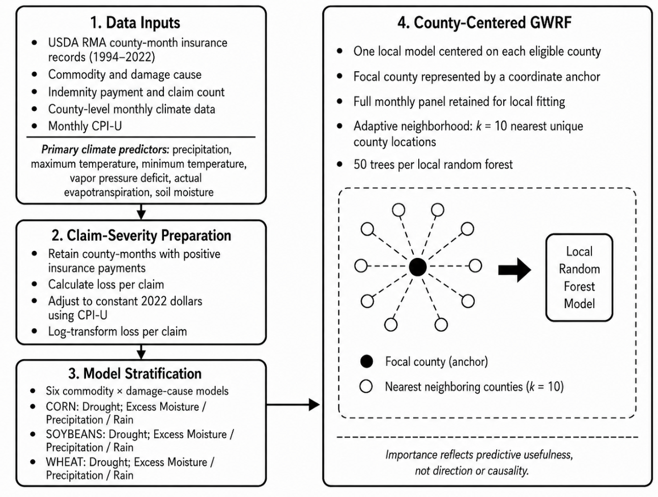
Figure 2.
County-centered geographically weighted random-forest workflow. Agricultural insurance records were joined to monthly TerraClimate and temporal predictors at the county–month scale. For each focal county, an adaptive neighborhood of unique county locations was selected, and all eligible monthly observations from those counties were used to fit a local random forest. County-specific permutation importance values were subsequently summarized and mapped.
Figure 2.
County-centered geographically weighted random-forest workflow. Agricultural insurance records were joined to monthly TerraClimate and temporal predictors at the county–month scale. For each focal county, an adaptive neighborhood of unique county locations was selected, and all eligible monthly observations from those counties were used to fit a local random forest. County-specific permutation importance values were subsequently summarized and mapped.
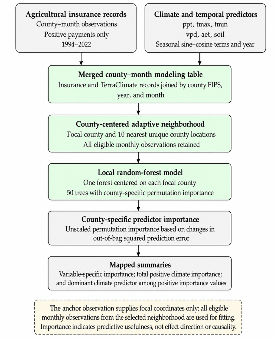
Figure 3.
Total positive climate importance for (A) corn drought, (B) corn excess moisture/precipitation/rain, (C) soybean drought, (D) soybean excess moisture/precipitation/rain, (E) wheat drought, and (F) wheat excess moisture/precipitation/rain. Values are the sum of positive local permutation importance across precipitation, maximum temperature, minimum temperature, vapor pressure deficit, actual evapotranspiration, and soil moisture. A common color scale is used across all six panels. Because the models were fitted separately, comparisons of raw importance magnitudes among models remain descriptive.
Figure 3.
Total positive climate importance for (A) corn drought, (B) corn excess moisture/precipitation/rain, (C) soybean drought, (D) soybean excess moisture/precipitation/rain, (E) wheat drought, and (F) wheat excess moisture/precipitation/rain. Values are the sum of positive local permutation importance across precipitation, maximum temperature, minimum temperature, vapor pressure deficit, actual evapotranspiration, and soil moisture. A common color scale is used across all six panels. Because the models were fitted separately, comparisons of raw importance magnitudes among models remain descriptive.
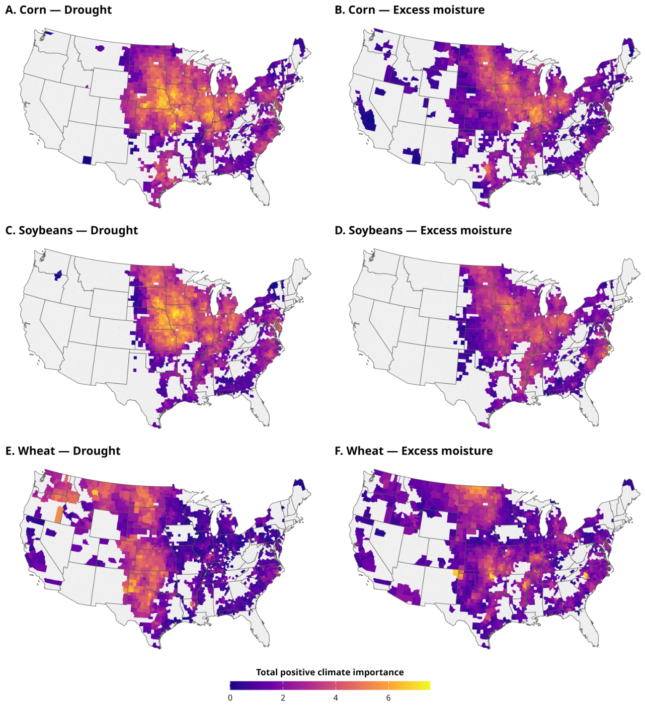
Figure 4.
Dominant local climate predictor for (A) corn drought, (B) corn excess moisture/precipitation/rain, (C) soybean drought, (D) soybean excess moisture/precipitation/rain, (E) wheat drought, and (F) wheat excess moisture/precipitation/rain. The mapped category is the climate variable with the highest positive permutation importance in each focal county. “No positive importance” indicates that all six local climate-importance values were nonpositive. Dominance does not convey effect direction or causality.
Figure 4.
Dominant local climate predictor for (A) corn drought, (B) corn excess moisture/precipitation/rain, (C) soybean drought, (D) soybean excess moisture/precipitation/rain, (E) wheat drought, and (F) wheat excess moisture/precipitation/rain. The mapped category is the climate variable with the highest positive permutation importance in each focal county. “No positive importance” indicates that all six local climate-importance values were nonpositive. Dominance does not convey effect direction or causality.
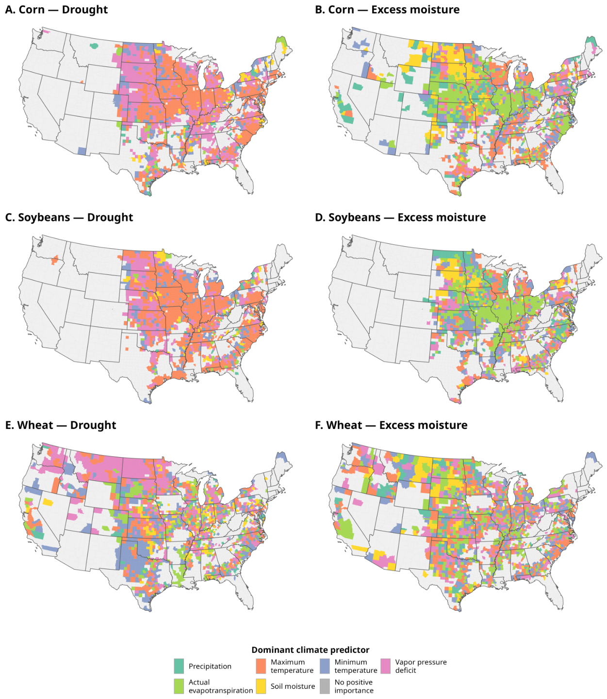
Figure 5.
County-centered local permutation importance for monthly maximum temperature in (A) corn drought, (B) corn excess moisture/precipitation/rain, (C) soybean drought, (D) soybean excess moisture/precipitation/rain, (E) wheat drought, and (F) wheat excess moisture/precipitation/rain. Positive values indicate greater local predictive usefulness. Negative values do not indicate a beneficial temperature effect. A common color scale is used across all six panels. Because the models were fitted separately, comparisons of raw importance magnitudes among models remain descriptive.
Figure 5.
County-centered local permutation importance for monthly maximum temperature in (A) corn drought, (B) corn excess moisture/precipitation/rain, (C) soybean drought, (D) soybean excess moisture/precipitation/rain, (E) wheat drought, and (F) wheat excess moisture/precipitation/rain. Positive values indicate greater local predictive usefulness. Negative values do not indicate a beneficial temperature effect. A common color scale is used across all six panels. Because the models were fitted separately, comparisons of raw importance magnitudes among models remain descriptive.
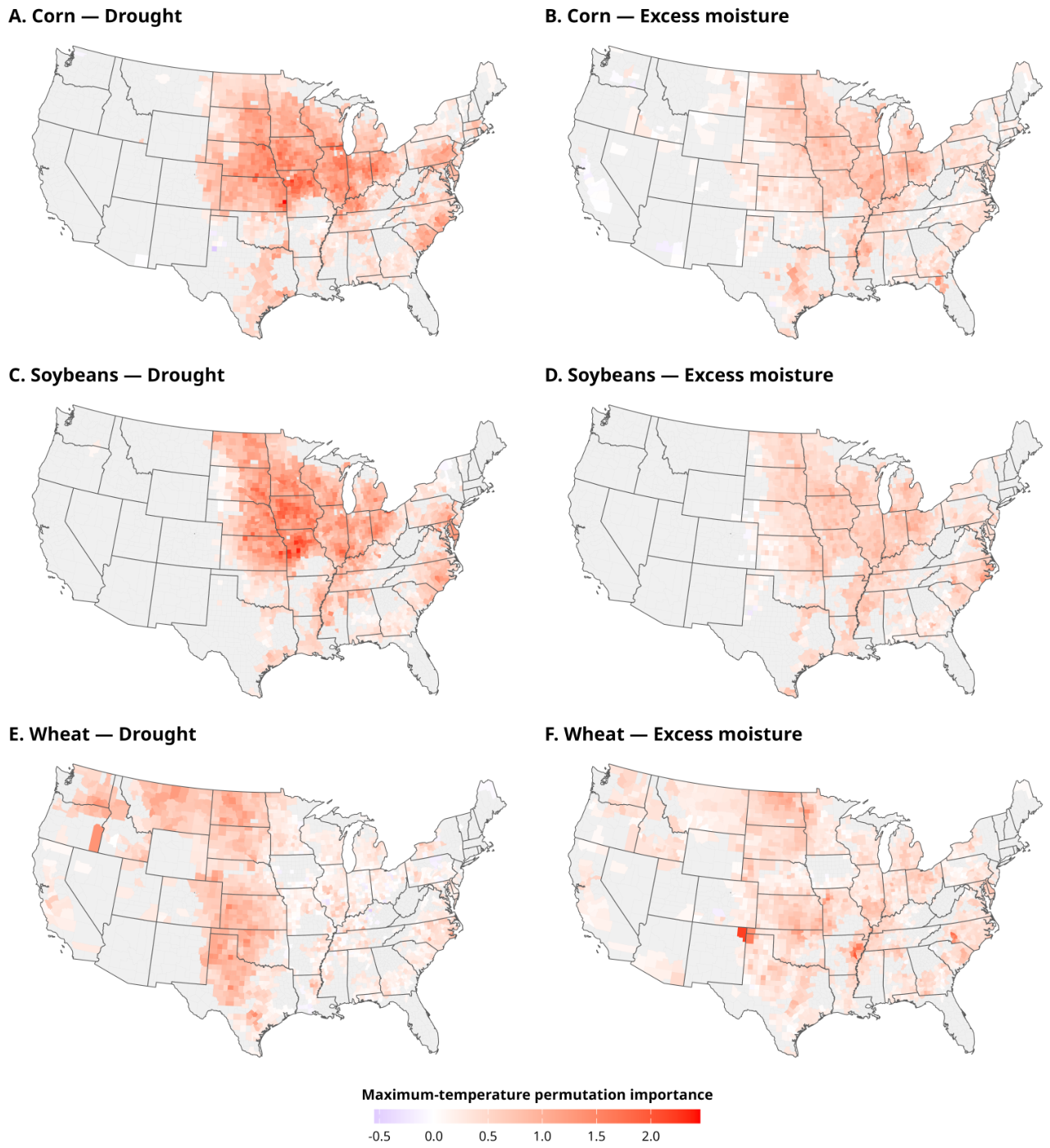

Table 1.
County–month coverage and local training support for the six primary county-centered GWRF models. The adaptive bandwidth was 10 unique county locations, and each local forest used 50 trees. Local training observations are the county–month records used to fit each county-centered random forest; mean, minimum, and maximum values summarize support across focal counties.
Table 1.
County–month coverage and local training support for the six primary county-centered GWRF models. The adaptive bandwidth was 10 unique county locations, and each local forest used 50 trees. Local training observations are the county–month records used to fit each county-centered random forest; mean, minimum, and maximum values summarize support across focal counties.
| Local training observations | |||||
|---|---|---|---|---|---|
| Model | County–months | Counties | Mean | Min | Max |
| Corn × Drought | 109,252 | 1,880 | 595.0 | 16 | 1,553 |
| Corn × Excess moisture | 121,159 | 1,934 | 635.8 | 19 | 1,841 |
| Soybeans × Drought | 108,877 | 1,722 | 646.6 | 25 | 1,471 |
| Soybeans × Excess moisture | 129,966 | 1,743 | 759.1 | 21 | 2,018 |
| Wheat × Drought | 74,527 | 1,797 | 426.4 | 14 | 2,187 |
| Wheat × Excess moisture | 80,789 | 1,921 | 428.9 | 35 | 1,932 |
Table 2.
Mean local permutation importance, with median in parentheses, for the six climate predictors. Rankings are most defensible within each model; raw magnitudes across separately fitted models are descriptive. Boldface identifies the predictor with the highest mean permutation importance within each model.
Table 2.
Mean local permutation importance, with median in parentheses, for the six climate predictors. Rankings are most defensible within each model; raw magnitudes across separately fitted models are descriptive. Boldface identifies the predictor with the highest mean permutation importance within each model.
| Model | ppt | tmax | tmin | vpd | aet | soil |
|---|---|---|---|---|---|---|
| Corn × Drought | 0.329 (0.330) | 0.765 (0.712) | 0.593 (0.569) | 0.712 (0.682) | 0.408 (0.408) | 0.372 (0.337) |
| Corn × Excess moisture | 0.354 (0.332) | 0.466 (0.440) | 0.447 (0.425) | 0.381 (0.371) | 0.464 (0.419) | 0.319 (0.263) |
| Soybeans × Drought | 0.315 (0.299) | 0.793 (0.766) | 0.591 (0.565) | 0.617 (0.579) | 0.409 (0.391) | 0.350 (0.304) |
| Soybeans × Excess moisture | 0.357 (0.348) | 0.487 (0.484) | 0.485 (0.482) | 0.413 (0.415) | 0.517 (0.498) | 0.304 (0.267) |
| Wheat × Drought | 0.220 (0.166) | 0.367 (0.288) | 0.367 (0.282) | 0.361 (0.277) | 0.277 (0.227) | 0.187 (0.153) |
| Wheat × Excess moisture | 0.250 (0.225) | 0.394 (0.357) | 0.379 (0.344) | 0.352 (0.315) | 0.363 (0.326) | 0.214 (0.177) |
Table 3.
Sensitivity of climate-importance results to the adaptive neighborhood bandwidth.
| Model | Total-importancePearson r | Dominant-predictoragreement (%) | Predictor-rank | Top predictor | Roughnessreduction (%) |
|---|---|---|---|---|---|
| Corn × drought | 0.882 | 57.3 | 1.000 | Max. temp. → Max. temp. | 23.3 |
| Corn × excess moisture | 0.873 | 44.1 | 1.000 | Max. temp. → Max. temp. | 22.0 |
| Soybeans × drought | 0.895 | 61.7 | 1.000 | Max. temp. → Max. temp. | 26.8 |
| Soybeans × excess moisture | 0.858 | 46.8 | 0.943 | AET → AET | 15.6 |
| Wheat × drought | 0.847 | 38.2 | 0.943 | Max. temp. → Min. temp. | 27.4 |
| Wheat × excess moisture | 0.792 | 34.8 | 1.000 | Max. temp. → Max. temp. | 21.7 |
Notes: Total-importance Pearson r compares county-level total positive climate importance between the k = 10 and k = 25 models. ominant-predictor agreement is the percentage of matched counties assigned the same highest-ranked positive climate predictor. Predictor-rank ρ is the Spearman correlation between the model-wide rankings of the six climate predictors. The arrow identifies the top-ranked predictor under k = 10 and k = 25, respectively. AET denotes actual evapotranspiration. Roughness reduction is the percentage decrease in standardized adjacent-county roughness under k = 25 relative to k = 10; larger values indicate greater spatial smoothing.
Disclaimer/Publisher’s Note: The statements, opinions and data contained in all publications are solely those of the individual author(s) and contributor(s) and not of MDPI and/or the editor(s). MDPI and/or the editor(s) disclaim responsibility for any injury to people or property resulting from any ideas, methods, instructions or products referred to in the content. |
© 2025 by the author. Licensee MDPI, Basel, Switzerland. This article is an open access article distributed under the terms and conditions of the Creative Commons Attribution (CC BY) license.
Copyright: This open access article is published under a Creative Commons CC BY 4.0 license, which permit the free download, distribution, and reuse, provided that the author and preprint are cited in any reuse.