
Submitted:
04 August 2026
Posted:
05 August 2026
You are already at the latest version
Abstract
As the development of deep oil and gas resources advances continuously, the role of weighted fracturing fluids in reducing wellhead operating pressure becomes increasingly important. However, the turbulent frictional drag behaviors of weighted fracturing fluids in pipes have not been understood systematically. The frictional drag characteristics and flow behaviors of non-weighted and weighted fracturing fluids in pipes are investigated at different flow rates, densities, pipe diameters, and rheological parameters via steady-state rheological tests and pipe flow friction experiments, together with large-eddy simulation and a power-law constitutive model for generalized Newtonian fluids. Main findings are as follows. The drag reduction rates of non-weighted polyacrylamide solutions basically increase with flow rate, and the optimal molecular weight of 600–700×104 corresponds to the highest drag reduction rate of 62%, while excessively large molecular weights weaken drag reduction effectiveness due to enhanced chain entanglement. The types of weighting salts have a significant effect on drag reduction performance. The 20% KCl system obtains the highest drag reduction rate of 64.8%, while the high-density CaBr2 system gets the lowest of 42.3% because high salinity suppresses the stretching of polymers. Parameter sensitivity analysis indicates that the power-law index n is the most sensitive parameter controlling frictional drag, followed by pipe diameter D. The novelty of this study lies in integrating experimental investigation, LES, and parameter sensitivity analysis to provide a theoretical basis for deep fracturing working conditions and fracturing fluids design.
Keywords:
weighted fracturing fluid
; turbulent frictional drag
; pipeline friction resistance test
; largeeddy simulation
; generalized Newtonian fluid
; sensitivity analysis
1. Introduction
As conventional oil and gas resources gradually become depleted, oil and gas exploration and development shift from middle and shallow formations to deep and ultra-deep ones. Hydraulic fracturing has developed into one of the core engineering technologies for improving the effective production degree of low-permeability and low-porosity reservoirs [1]. In the process of hydraulic fracturing, the frictional drag along the pipe increases rapidly with the increasing well depth or flow rate, which may lead to an excessively high wellhead pressure [2,3]. In engineering practice, weighted fracturing fluids are often employed to reduce the wellhead pressure. By adding inorganic- or organic-salt weighting agents into water-based fracturing fluids, the hydrostatic pressure in the wellbore increases, thereby lowering the surface pump pressure [4]. The weighting agents commonly used in existing studies include CaCl2, KCl, NaCl, sodium formate, and other organic-salt systems. Weighting agents not only alter the densities of fracturing fluids, but also influence the hydration, crosslinking reaction, and shear-thinning behaviors of polymers, so that weighted fracturing fluids exhibit different rheological characteristics from conventional fracturing fluids [5,6]. Therefore, understanding the turbulent frictional drag behaviors of weighted fracturing fluids in pipes is of great significance for the parameter optimization of deep fracturing systems and the prediction of wellhead pressures.
Water-based fracturing fluids are classified as non-Newtonian fluids containing polymers, crosslinking networks, or surfactant structures, with an apparent viscosity varying with shear rate. They may exhibit shear-thinning, viscoelastic, and other rheological behaviors [7,8]. Toms [9] was the first to discover that adding a small amount of long-chain polymer to Newtonian fluids can significantly reduce the turbulent frictional drag. This phenomenon is widely known as the Toms effect. Based on abundant pipe flow experimental data, Virk [10] proposed the maximum drag reduction asymptote, revealing that the friction factor of polymer solutions is essentially different from the Blasius empirical relationship for Newtonian fluids. Lumley [11] elucidated the drag-reducing mechanisms based on the influence of polymers on small-scale turbulent structures and viscous effects. Choueiri et al. [12] further pointed out that the elastic effect of polymers may cause drag reduction to exceed the conventional asymptotic limit.
In terms of experimental studies, Escudier et al. [13] carried out turbulent flow experiments in circular pipes to investigate the drag reduction behaviors of various polymer solutions, revealing a close correlation between the frictional drag variation of polymer solutions and their viscoelasticity and the extensional viscosity at low shear/strain rates. Donohue et al. [14] conducted near-wall dye flow visualization experiments, suggesting that polymer additives can alter the structures of the viscous sublayer and near-wall region, thereby influencing the generation process of turbulent kinetic energy in wall turbulence. White et al. [15] provided an overview of the research on polymers for turbulent drag reduction, pointing out that high-molecular-weight polymers can achieve drag reduction by altering near-wall turbulent structures, suppressing Reynolds shear stress and regulating turbulent energy dissipation. Motozawa et al. [16] investigated the streamwise process of drag reduction in polymer solutions using the particle image velocimetry technique, revealing that turbulent structures, Reynolds shear stress and wall-normal turbulent intensity undergo significant changes after polymer injection. In the context of hydraulic fracturing, Le Brun et al. [17] studied the drag reduction effectiveness and shear stability of a modified acrylamide copolymer. Habibpour et al. [18] evaluated the turbulent drag reduction performance and shear degradation characteristics of hydrolyzed polyacrylamide (HPAM)/xanthan gum polymer blends using a closed-loop circulation system. Wang et al. [19] and Jing et al. [20,21] investigated the influence of molecular structure, concentration, and salinity of hydrophobically associating polymers and HPAM with ultra-long side chains using a friction test apparatus.
In terms of weighted fracturing fluids, Qiu et al. [22] and Gupta et al. [23] carried out laboratory evaluation on high-density brine-based fracturing fluids and studied their applications to deep/ultra-deep fracturing, suggesting that weighted systems can decrease the wellhead operating pressure by increasing the hydrostatic pressure. Different weighted systems were evaluated in terms of density control, crosslinking delay, rheological stability, temperature and shear resistance, and drag reduction, providing an experimental basis for the design of weighted fracturing fluid systems for high-temperature, high-pressure deep reservoirs [24,25,26,27,28]. Liang et al. [29] proposed a field-scale performance prediction method for drag reducers based on laboratory friction tests, emphasizing the similarity between laboratory parameters (pipe diameter, flow rate, and Reynolds number) and field working conditions. These studies indicate that the changes in the frictional drag of fracturing fluids are the result of fluid apparent viscosity variation, as well as the regulating effect of polymers, weighting salt types, and crosslinking structures on near-wall turbulent structures.
Compared with experiments, numerical simulation can capture flow fields and friction characteristics of fracturing fluids in pipes at a lower cost. In direct numerical simulation (DNS) studies, the Navier-Stokes equation is coupled with a viscoelastic constitutive equation to directly resolve the interaction between elastic stress and turbulent structures [30,31,32]. Oldroyd-B, FENE-P, and Giesekus are commonly used constitutive models [30,31]. Recently, DNS has also been used to research the transition mechanisms of elasto-inertial turbulence and viscoelastic fluids. The findings indicate that polymer elasticity not only weakens the conventional inertial turbulence, but also may induce new elastically unstable structures [33,34]. When DNS is employed, however, all turbulent scales and polymer stress fields have to be resolved, leading to extremely high computational costs. In addition, some parameters of viscoelastic constitutive models such as FENE-P can hardly be obtained directly from experiments. In engineering flow applications, the generalized Newtonian fluid (GNF) model is widely applied to simulate non-Newtonian fluids in pipes, for it can be directly correlated with rheological experimental data. In the GNF model, fluid viscosity is expressed as a function of shear rate, which can be described using the power-law, Cross, or Carreau model [35,36].
In addition to DNS, Reynolds-averaged Navier-Stokes (RANS) and large-eddy simulation (LES) methods are also widely applied to simulate non-Newtonian and viscoelastic fluids, as their computational costs are relatively low. Malin [37] employed the modified k-ε model to investigate the turbulent flow of power-law fluids in pipes, demonstrating that the turbulent model modified with a viscosity function and damping can be used to compute the frictional drag of certain non-Newtonian fluids. Based on the framework of GNF, Pinho and Cruz [38,39] developed a low-Reynolds k-ε model suitable for drag-reducing fluids. Furthermore, k-ε-v²-f, k-ω, and pseudo-elastic stress were modified, respectively, to improve the ability of RANS to predict turbulent kinetic energy and friction factor [40,41,42]. Gnambode [43] employed LES to study the turbulent flow of power-law fluids in pipes, suggesting that LES can be used to capture the changes in the near-wall turbulent structures and frictional drag of shear-thinning fluids. Amani et al. [44] pointed out that non-Newtonian stress and apparent viscosity fluctuation should not be neglected in the LES of turbulent non-Newtonian fluids. Taghvaei and Amani [45] demonstrated that the simulation of high-Reynolds pipe flow of non-Newtonian fluids shall pursue a balance between accuracy and computational cost. To sum up, LES can resolve large-scale turbulent structures and deal with small-scale fluctuations using the subgrid-scale model, so it is more suitable for analyzing the near-wall turbulent structures and friction-generating mechanisms in non-Newtonian pipe flow.
Previous studies on the friction behaviors of fracturing fluids in pipes mostly focused on the influence of polymer concentrations, types, and molecular structures. In engineering practice, however, the near-wall turbulent structures and friction behaviors of weighted fracturing fluids in pipes have not been comprehensively investigated, even though they may be crucial to the design of high-performance weighted fracturing fluids. This study combines rheological experiments, pipe flow friction tests, and three-dimensional numerical simulations of non-Newtonian turbulent flows, with a focus on the effects of different weighted salt systems on the in-pipe flow field, near-wall turbulent structures, and frictional drag characteristics, and further analyzes the sensitivity of key factors to pipe flow friction. It provides theoretical guidance for system optimization in deep and ultra-deep fracturing operations.
2. Experimental Methodology
2.1. Preparation of Fracturing Fluids
A variety of non-weighted and weighted fracturing fluids were selected as experimental objects for rheological and pipe flow friction experiments for fracturing fluids. The experimental materials mainly include fresh water, Polyacrylamide (PAM), KCl, CaCl2, CaBr2, temperature stabilizer, cleanup additive, demulsifier, and cosolvent. PAM polymer solution served as non-weighted fracturing fluid. Different mass fractions of PAM were added slowly and uniformly to fresh water, which acted as the base fluid, and then stirred continuously for sufficient swell and hydration until the solution turned uniform. Following this process, 12 kinds of fracturing fluids with various polymer molecular weights and zero-shear viscosities η0 were prepared, with polymer molecular weights mainly ranging from 4×10⁶ to 9×10⁶ and η0 ranging from 60 to 84 mPa·s. This group of samples can be used to analyze the influence of polymer chain length and zero-shear viscosity on pipe friction.
Four kinds of weighted fracturing fluids were prepared by adding inorganic salts to water-based fracturing fluids to regulate their density, seeing Table 1. Weighted fracturing fluid systems are used to investigate the influence of weighting salt type, concentration, and system density on friction behaviors. In the process of fluid preparation, weighting salts and fresh water were weighed as per experimental formulations (1 L solution), and then poured into a stirring vessel. The constant-speed stirrer was started. After the salts were completely dissolved, the relevant additives and polymers were added successively, while the stirring was maintained to ensure the system was mixed sufficiently. In this way, the corresponding fracturing fluid system was prepared.
2.2. Pipe Flow Friction Test
The pressure difference method is adopted in the experiments to drive fracturing fluids to stably flow through the test pipe section at a given pipe diameter and length and flow rate. The inlet pressure and outlet pressure were measured, and their difference was the pressure drop along the pipe section. To evaluate the drag reduction effectiveness of fracturing fluids compared with fresh water, the drag reduction rate DR is defined under the identical flow rate condition:
(1)
where ΔP0 and ΔP1 are the pressure drops of fresh water and fracturing fluid, respectively, in kPa. DR>0 indicates that fracturing fluids exhibit drag reduction effectiveness compared with fresh water, while DR<0 indicates drag increase.
Pipe flow friction tests were carried out at 25℃. A 12.7 mm × 3 m straight pipe is used as the test pipe section. The test system is composed of a mixing tank, agitator, screw pump, straight pipe section, flowmeter, pressure sensor, data acquisition system, and waste liquid tank. The sketch of the test system is shown in Figure 1. The well-prepared and uniform fracturing fluids were added to the mixing tank and maintained uniformly using the agitator, as shown in the physical photo in Figure 2(a). The visual control panel was accessed via the computer control system to set up test pipe diameter, pressure difference range, expected flow rate, sampling frequency, and test time. After parameter setup, the screw pump was started to pump the test fluids from the mixing tank to the straight pipe section. Data recording began when the flow rate became stable. A flowmeter is used for the real-time monitoring of flow rates at the pipe inlet, as shown in the physical photo in Figure 2(b). During the tests, the flow rate was initially 10 L/min and then increased at the rate of 5 L/min until the highest value of 90 L/min was reached. The corresponding pressure difference was recorded after the flow rate became stable. The flow rate, pressure difference, and temperature were recorded synchronously using the data acquisition system. After one sample was tested, the system was cleaned for another sample test. After all tests were completed, the experimental data were output for calculating the frictional drag and DR of fracturing fluids in pipes.
2.3. Rheological Test
Fracturing fluids are non-Newtonian fluids, whose viscosity is not constant but varies with shear rate. Therefore, zero-shear viscosity alone can hardly provide an accurate description of the real rheological behaviors of fracturing fluids during high-shear flow in pipes. To support the pipe flow friction tests, it is necessary to carry out steady-state shear tests to understand the rheological behaviors of fracturing fluids and the change patterns of apparent viscosity at various shear rates. During the test process, the rheometer applies shear force on samples by rotating the rotator, and records the stress response of each sample. In principle, it converts the angular displacement and velocity of motor rotation into strain and shear rate, and the measured torque into shear stress. Thereby, the apparent viscosity of samples at various shear rates can be calculated based on the relationship between shear stress and shear rate, seeing Equation (2).
(2)
where η is the apparent viscosity, Pa·s, τ is the shear stress, Pa, and γ is the shear rate, s-1.
Thermo Scientific HAAKE MARS60 rotary rheometer and its supporting control system were employed, as shown in Figure 3. Before testing, the air compressor and host rheometer were started, and the temperature control system and measurement rotator were confirmed to be normal. The steady-state shear test procedure was set according to the experiment plan via HAAKE RheoWin software, with the shear rate in the range of 0.1–1000 s-1, and the test temperature being stable. Multiple data points were acquired continuously, and their average was taken as the η at each level of shear rate. After all samples were tested, the data of shear rate, shear stress, and η were output, and the measurement system was cleaned.
3. Numerical Simulation Methods
3.1. Governing Equations
It is assumed that the flow of fracturing fluids in a cylindrical pipe is three-dimensional, transient, and incompressible, and the fluid density ρ remains constant. The continuity equation and momentum equation are
(3)
and
(4)
where u is the velocity vector, m/s, p is the static pressure, Pa, and τ is the viscous stress tensor.
In view that DNS has excessively high computational costs and the RANS method struggles to resolve the near-wall turbulent fluctuations and may impact the prediction accuracy of frictional resistance at medium Reynolds numbers, this study employs the LES method in numerical simulation and applies the finite volume method to spatial discretization. In LES, turbulent motion is divided through spatial filtering into large-scale analyzable structures and small-scale non-analyzable fluctuations. Large-scale eddies are solved directly via governing equations, while the influence of small-scale eddies is enclosed with a sub-grid scale (SGS) model. In this study, the Wall Adaptive Local Eddy Viscosity (WALE) model [46] was selected as the SGS model, which can reasonably describe the attenuation characteristics of eddy viscosity near the wall and is suitable for turbulent flow constrained by the inner pipe wall. The second-order upwind and second-order discretization are used for the discretization of the momentum equation and pressure field. The second-order implicit method is adopted for the time discretization. The pressure-velocity coupling is dealt with the coupled algorithm.
3.2. Rheological Model
The tests of weighted fracturing fluids for engineering practice indicate that their viscosity varies with strain rate. To accurately describe the rheological behaviors of the weighted fracturing fluids, this study employed the GNF constitutive model to describe the viscous stress tensor of fluids. Different from Newtonian fluids, the apparent viscosity in the GNF model is not a constant, but a function of shear rate. Therefore, the viscous stress tensor can be expressed as:
(5)
where is the viscosity function, D is the strain rate tensor, which is defined as
(6)
and is the shear rate, expressed as . Therefore, the viscous stress tensor in the GNF model can be expressed as
(7)
In the Power-Law model, the viscosity function is
(8)
where K is the consistency coefficient, representing the measurement of fluid viscosity at unit shear rate; n is the rheological index, determining the deviation degree and direction of fluid from Newtonian behavior, n<1: shear thinning, n>1: shear thickening.
3.3. Computational Domains and Boundary Conditions
A fluid simulation platform that can predict the frictional drag of viscoelastic fracturing fluids under actual working conditions was established. A computational domain for the flow in circular pipes was established for numerical simulation by referring to the experimental model size listed in Sorgun et al. [47], as shown in Figure 4. The mesh partitioning method and mesh accuracy for viscoelastic fluids should be consistent with those for Newtonian fluids. A cylindrical coordinate system is used, with z, r, and θ representing axial flow direction, wall normal direction, and circumferential angle, respectively. Periodic boundary conditions were applied in the streamwise direction to ensure that stable and fully developed pipe flow can be obtained in a small computational domain. The required minimum pipeline length for the streamwise length was estimated based on the following formula.
(9)
where C is set to 2000 based on experience, is the viscosity, Pa·s, is the density, kg/m3, and is the friction velocity, , m/s.
The non-slip boundary conditions were applied to the wall, without considering the influence of wall roughness and gravity. The structured hexahedral grid was employed in the spatial discretization. The meshes in the streamwise and circumferential directions (r and θ) are divided uniformly. O-grid division method is used in the wall-normal direction. To evaluate the influence of grid scale on computational results and determine the optimal grid distribution that meets the required computational accuracy, a grid independence study is conducted. The averaged dimensionless velocity distributions in the radial direction at four grid resolutions are obtained and compared with DNS results illustrated in reference [48], as shown in Figure 5. The ultimate grid meets the following requirements: the grid scale of the first layer on the wall rmin+ < 1, the radial grid scale Δrmax+ ≤ 10, the streamwise and circumferential grid scales Δz+ ≤ 10 and Δ(rθ)+ ≤ 10, where the superscript "+" represents the result normalized by the wall unit. The comparison results demonstrate that the computational grids have met the requirement of grid independence.
A user-defined function is established for the obtained apparent viscosity, enabling the viscosity to be updated in real time according to the shear rates during the computation process, to fully capture the shear rheological behaviors of weighted fracturing fluids. The computation is considered to be converged when the residuals of all variables in the simulation equations drop below 10-5.
3.4. Validation of Numerical Model
The complexity and uncertainty inherent in the experimental data of coiled tubing hinder their direct application to the validation of numerical simulation results. Thus, we adopt the experimental data from Sorgun et al. [47] under similar fluid properties and flow conditions to validate the numerical method, as shown in Figure 6. The corresponding dimensionless generalized Reynolds number () ranges from 3600 to 4600. It indicates that the numerical simulation results are overall in good agreement with the experimental data, with an average relative deviation of about 10% and a minimum of around 5%. From an engineering perspective, the above discrepancy is within the acceptable range, hence confirming the accurate prediction of turbulent fracturing fluids' frictional drag by the established numerical model. It should be noted that the discrepancies are mainly induced by the GNF model. Despite this, the present results are generally consistent with the recent findings in reference [49], suggesting the good applicability of this model.
It should be noted that all simulated conditions are in the turbulent regime. Figure 7 shows the comparison of axial and radial root-mean-square fluctuating velocity urms+ and vrms+ along the wall-normal direction between LES results and the DNS data [48]. The distribution of urms+for the power-law fluids is generally consistent with the DNS results, except for some discrepancies near the peak and in the outer layer. The radial velocity fluctuations of power-law fluids are obviously affected by rheological behaviors and shows different from the DNS data. At moderate Reynolds numbers of 4128, vrms+ is characterized by a lower degree of turbulent fluctuations and shows features of early turbulence. The employed numerical method demonstrates good capability of predicting turbulent statistics in pipes.
4. Results and Discussions
4.1. Friction Characteristics of Fracturing Fluids
(1) Friction characteristics of non-weighted fracturing fluids
The pressure drop data of 12 kinds of PAM solutions at various flow rates were acquired and compared with the results of fresh water. Figure 8 shows the variation of the frictional pressure drop and drag reduction rate of PAM solutions with different molecular weights at a zero-shear viscosity η0 of 84 mPa·s. As the flow rate increases from 10 to 90 L/min, the pressure differences of fresh water and PAM solutions all increase gradually, and the frictional drag along the pipe increases. Compared with fresh water, PAM polymer solutions have a slower increase in pressure difference. At the stage of low flow rate (10–30 L/min), the frictional pressure drop of PAM solutions is larger than that of fresh water. It indicates that polymer molecular chains are not stretched sufficiently, viscosity resistance is dominant, and a drag increase characteristic appears. When the flow rate exceeds 30 L/min, the frictional pressure drop of PAM solutions is smaller than that of fresh water; the drag reduction rate transforms from negative to positive, indicating drag reduction occurs. As the flow rate increases, the drag reduction rate increases continuously, suggesting that at high flow rates and strong shear force, PAM molecular chains stretch enough to suppress the turbulent fluctuations in pipes, thus decreasing the pressure drop.
Regarding the influence of molecular weights, PAM solutions are basically consistent in the variation trend of pressure drop at the identical zero-shear viscosity, but differ in drag reduction effectiveness at high flow rates. The PAM solutions with small or medium molecular weights have relatively low frictional drag, with the maximum drag reduction rate up to 62%, while those with molecular weights of 800×104 to 900×104 have relatively high frictional pressure drop, with the maximum drag reduction rate of 56%. It suggests that under the conditions of this experiment, the PAM solutions with moderate molecular weights perform better in reducing frictional drag, while those with excessively large molecular weights may enhance the entanglement between polymer molecular chains and the internal viscous energy dissipation, thereby weakening the drag reduction effectiveness.
Figure 9 shows the variation of frictional drop and DR of PAM solutions with η0 of 60 mPa·s, 66 mPa·s, and 84 mPa·s, respectively, under the identical molecular weight of 600×104 to 700×104. PAM solutions with various η0 all exhibit DR increasing with flow rate. At low flow rates, DR is relatively low, and with the increasing flow rate, it increases rapidly. In the stage of high flow rate, the DR of PAM solutions increases slowly and gradually approach to be stable, with the maximum value ranging from 60% to 62%. The PAM solution with η0 = 60 mPa·s exhibits the lowest pressure drop and the highest DR, while that with η0 = 84 mPa·s is contrary. It suggests that the drag reduction effectiveness of PAM solutions is not enhanced simply by increasing η0, but is also influenced by viscous resistance and molecular chain stretching. An appropriate decrease in zero-shear viscosity is conducive to the reduction of frictional drag in pipes.
(2) Friction characteristics of weighted fracturing fluids
The pressure drop of four kinds of weighted fracturing fluids at various flow rates was acquired in the friction experiments and was compared with the results of fresh water to calculate the DR of each formulation system. The densities of weighted fracturing fluids are 1150 kg/m3, 1150 kg/m3, 1350 kg/m3, and 1500 kg/m3, respectively. Figure 10 shows the variation of pressure drop and DR of each system with flow rate. Even though their pressure drops increase with flow rate, four kinds of weighted systems still exhibit certain drag reduction behaviors compared with fresh water. At the maximum flow rate of 90 L/min, the DRs of 20% KCl, 25% CaCl2, 46% CaCl2, and 53% CaBr2 systems are 64.77%, 57.72%, 49.36%, and 42.29%, respectively. Among these formulations, the 20% KCl system has the smallest pressure drop, and the 53% CaBr2 system has the largest one. It indicates that from the perspective of drag reduction effectiveness, the KCl system is the best, followed by the CaCl2 system, and the CaBr2 system is the worst. The reasons for this phenomenon are: the KCl system has relatively low density and high polymer dosage, promoting the role of polymer molecular chains in drag reduction; the CaCl2 and CaBr2 systems have relatively high salinity and density, resulting in high frictional drag, as high salinity impacts the stretching state of polymer molecular chains and high-density fluids exhibit enhanced inertia flowing in pipes. It suggests that the drag reduction performance of weighted fracturing fluids is under the joint influence of salt type and concentration and system density. As weighting salt concentration and density increase, the drag reduction of polymer molecular chains is suppressed. It is worth noting that while weighted fracturing fluids exhibit generally lower drag reduction than pure PAM solutions in Figure 9(b), their higher density results in higher hydrostatic pressure, which is advantageous for lowering surface pump pressure in field applications.
4.2. Rheological Characteristics of Fracturing Fluids
(1) Rheological characteristics of non-weighted fracturing fluids
Figure 11 shows the variation of apparent viscosity of different PAM solutions at various shear rates. Twelve groups of samples all exhibit obvious shear-thinning characteristics. At low shear rates of 0.1–1 s-1, η is relatively high, indicating strong entanglement and structural viscosity of polymer molecular chains. As the shear rate increases gradually, the entanglement degree of polymer molecular chains decreases, and η drops rapidly. When the shear rates enter the medium-high shear zone of 10–500 s-1, the viscosity decline slows down. When the shear rates reach 500–1000s-1, the viscosity of most samples approaches stability.
The sample comparison results indicate that the samples with higher zero-shear viscosity have higher η. At low shear rates, the samples with η0 = 84 mPa·s exhibit the highest viscosity, followed by those with η0=66 mPa·s and η0=60 mPa·s. Furthermore, with the increasing PAM molecular weights, η of the solution increases overall, indicating that the PAM with large molecular weights has strong viscosity-enhancing capacity and molecular chain entanglement. At high shear rates, however, the viscosities among different samples tend to be consistent, indicating that strong shear effect can mitigate the influence of η0 and molecular weight on η.
This rheological law is consistent with the friction test results. At low flow rates, the shear effect in pipes is weak, and the PAM solution maintains a high η, so viscous resistance performs as a dominant factor. Some samples may exhibit low drag reduction rates. As the flow rate rises, the average flow velocity and wall shear rate in the pipe increase, and the PAM solution undergoes shear thinning, thereby reducing the flow resistance. Consequently, the pressure difference is lower than that of fresh water, and the drag reduction rate gradually increases and tends to stabilize.
(2) Rheological characteristics of weighted fracturing fluids
Figure 12 shows the apparent viscosity of 4 kinds of weighted fracturing fluids at varying wall shear rate. All of these weighted fracturing fluids present certain shear-thinning characteristics. At low shear rates, the initial η of weighted fracturing fluids is lower than that of non-weighted PAM solutions. It indicates that high-concentration salt ions weaken the hydration expansion and entanglement of polymer molecular chains, thereby decreasing the system viscosity. As the shear rates increase, the polymer molecular chains gradually orient under shear action, resulting in a decrease in entanglement degree and η. At medium shear rates, the viscosity of each system decreases to a lower level.
The formation comparison results show that formulations 1 and 2 have higher polymer content, and their apparent viscosities are overall higher than those of formulations 3 and 4. As the shear rates increase, the viscosity differences among these formulations decrease gradually. It indicates that strong shear effect mitigates the influence of polymer concentration and weighting salt type on η. It should be noted that at high shear rates of 500–1000 s⁻¹, the viscosity of weighted fracturing fluids doesn’t continue to decline obviously, but increases or fluctuates slightly. This phenomenon may be caused by the conformational adjustment of polymer molecular chains, changes in hydration state, and high shear rheological response in high-concentration salt environments.
Besides, the power-law fluid F-1 used for numerical model validation is also shown in Figure 12. The rheological behavior between the four weighted fracturing fluid formulations and the F-1 fluid indicates that the viscosity of the F-1 fluid generally falls within the curve range of the actual fracturing fluids, confirming the comparability between numerical simulation and experiments.
4.3. Average Axial Velocity
Figure 13 shows the average axial velocity profiles normalized by the friction velocity for different densities, pipe diameters, K, and n, which all exhibit the turbulent velocity distribution characteristics of increasing rapidly in the near-wall region and slowing down gradually after the buffer layer. As the fluid density increases from 1009.6 kg/m3 to 1400 kg/m3 in Figure 13(a), the velocity profiles tend to shift upward in the logarithmic and outer layers, while remaining almost unchanged in the near-wall viscous region. Under the same flow conditions, an increase in density enhances liquid inertia and thus the turbulent momentum transport, leading to an increase in axial velocity in the outer layer. As the pipe diameter increases from 35 mm to 100 mm in Figure 13(b), the dimensionless axial velocity exhibits a decreasing trend after entering the buffer layer and the logarithmic layer. With the increasing pipe diameter, the flow scale increases, and the wall shear effect on the unit fluid weakens, leading to a change in the velocity gradient and consequently a descending velocity distribution. As the consistency coefficient K increases from 0.04 to 0.3 in Figure 13(c), the velocity profiles overall exhibit a slight descending trend. The consistency coefficient K reflects the viscous resistance level of fluids, and its increase results in a higher η under the same shear conditions, which enhances the viscous dissipation effect during the flow process, thereby reducing the momentum transport capacity of fluids and shifting the velocity profiles downward. As n increases from 0.55 to 0.85 in Figure 13(d), the velocity profile gradually shifts downward, with a lower n corresponding to a higher dimensionless axial velocity. The reason is that n determines the shear-thinning degree of the fluid. When n decreases, the non-Newtonian shear-thinning effect is enhanced, and η and flow resistance in the near-wall region with high shear rates decrease, consuming less fluid momentum, thus shifting the velocity profile upward.

4.4. Flow Field Analysis
The influences of flow condition and physical property parameters on the turbulent structures of weighted fracturing fluids in pipes are obtained and analyzed. The power-law index n directly characterizes the fluid shear-thinning behaviors, and its variation has a more significant impact on the turbulent structure and velocity distribution than other parameters. So, n is selected as a typical parameter, and the flow fields at n = 0.85 and 0.55 are analyzed.
Figure 14 shows the cross-section contour of streamwise velocity captured near the wall (x=−0.0209 m) at a flow rate of 320 L min−1. At n=0.85, the overall velocity near the wall is relatively low, the area of the high-velocity core region is small, and the streaky structures are dispersed and discontinuous, corresponding to a low shear rate. From the vortices presented by Q criterion isosurfaces and colored by velocity values shown in Figure 15, at n=0.85, there is a relatively large low-velocity region near the wall, and the turbulent structures in the flow field are large in scale and relatively regular in spatial distribution. Furthermore, the flow vorticity contours on the cross-section were compared, as shown in Figure 16. At n=0.85, the vortices are mainly distributed near the wall, and the vortex intensity is relatively low. It indicates the turbulent energy dissipation is weak. With a higher apparent viscosity at the wall, the viscous energy dissipation is strong. The DR results indicate that the latter effect plays a dominant role in this case, leading to an increased friction drag. At n=0.55, the velocity near the wall is overall higher in Figure 14; the high-velocity core region covers a larger area, and the streaky structures are longer and more continuous. In Figure 15, the high-velocity region extends from the pipe center toward the wall, the velocity gradient and the near-wall velocity increase, and the turbulent structures in the flow field are small-scale and distributed randomly. In Figure 16, the vortices extend from the vicinity of the wall toward the central pipe, the vorticity fluctuations are relatively intense, and the vortex intensity near the wall is higher. The above all indicate that the fluid has developed into a typical turbulent region with pronounced turbulent effects. The near-wall shear rate is higher, and the apparent viscosity decreases, which significantly reduces the frictional drag.
4.5. Sensitivity Analysis
Sensitivity analysis was conducted on the key factors influencing the friction factor. The flow rate q, power-law index n, consistency coefficient K, fluid density ρ, and pipe diameter D were selected as independent variables. The logarithmic regression elasticity coefficient method, the parameter perturbation verification method, and the partial correlation coefficient (PCC) method were applied jointly for cross-validation to identify the dominant factors influencing frictional drag in pipes.
Based on the power function relations of friction factor to various influence parameters, a logarithmic linear regression model was established as:
(11)
where C is a constant, a1, a2, a3, a4, a5 represent the elasticity coefficients corresponding to each parameter, expressed as:
(12)
In physics, it means that the friction factor f changes by ai% on average when the parameter xi increases by 1%.
As shown in Figure 17, the model predictions are in good agreement with the actual values, with a coefficient of determination R2 of 0.968. It indicates that the model can accurately reveal the variation patterns of the friction factor within the investigated parameter range. The distribution of the elasticity coefficients for each parameter was derived from the regression results. As shown in Figure 18, the parameter sensitivity is in the order of n>D>ρ>Q>K, and the sign indicates the direction of the influence of the parameters on f. It indicates that fluid rheological properties and pipe geometry are the primary factors controlling the variation of pipe frictional drag.
To test the stability of the regression analysis results, four representative base cases were further selected, as shown in Table 2, and local perturbations of ±1%, ±3%, and ±5% were applied to each parameter. Figure 19 shows the variation magnitudes in the friction factors caused by the perturbations of each parameter, which presents a ranking of parameter sensitivity as n>D>Q>ρ≈K. The sensitivity rankings in four base cases show good consistency, confirming the credibility of the sensitivity ranking results.
Considering the possible correlations among the input parameters, the PCC method is employed to analyze the independent influence of each parameter on the friction factor while keeping other variables constant. The system is supposed to contain five input parameters X1, X2, X3, X4, and X5, with Y being the response variable. The partial correlation coefficients can be calculated from the inverse matrix of the covariance matrix. Letting the inverse matrix of the joint covariance matrix be , the partial correlation coefficient between the i-th parameter and the response variable can be expressed as
(13)
where ωi, Y is the element in the i-th row and Y-th column of the inverse matrix Ω, ωi, i, ωY, Y are the corresponding diagonal elements, and the PCC value range is 0-1. The closer to 1, the more pronounced the influence of the parameter on the response variable.
Figure 20 shows the absolute values of partial correlation coefficients that indicate the influence of each parameter on friction factor. The parameter sensitivity is ranked as n>D>Q>K>ρ. Therefore, different methods exhibit some discrepancies in the rankings of flow rate, density, and consistency coefficient, for they handle parameter correlations and local nonlinear responses in different modes. From the integrated results obtained by the three methods, the sensitivity ranking of pipe friction factor is ultimately n>D>{Q,ρ}>K. It is suggested that during the pipeline transport of fracturing fluids, priority should be given to the control of fluid power-law index and the selection of an appropriate pipe diameter.
5. Conclusions
Focusing on the turbulent frictional behaviors of weighted fracturing fluids in pipes for deep oil and gas development, this paper systematically investigated the frictional behaviors of non-weighted and weighted fracturing fluids under various flow conditions by using pipe flow experiments, rheological tests, and LES. The influences of rheological parameters, fluid density, pipe diameter, and flow rate on frictional drag were revealed, and parameter sensitivity analysis was carried out for the cross-validation between experiments and numerical simulations. The main conclusions are as follows:
(1) For unweighted fracturing fluids, the polymer molecular weight and zero-shear viscosity exhibit optimal intervals for drag reduction. Under the same zero-shear viscosity, the PAM solution with a medium molecular weight of 600×104–700×104 achieves the best drag reduction effectiveness, with a maximum drag reduction rate of 62%. However, when the molecular weight is too high at 800×104–900×104, molecular chain entanglement intensifies, leading to an increase in viscous energy dissipation and a decrease in the drag reduction rate to 56 %. The lower the zero-shear viscosity, the higher the drag reduction rate at high flow rates. However, the differences among samples with various viscosities gradually diminish as the flow rate increases.
(2) For weighted fracturing fluids, the drag reduction performance is under the joint control of weighting salt type and system density. Among the four weighted systems, the 20% KCl system exhibits the best drag reduction effectiveness, that is, a 64.8% drag reduction rate at 90 L/min, followed by the CaCl2 systems of 57.7% and 49.4%, and the CaBr2 system gets the lowest drag reduction rate of 42.3 %. High-concentration salt ions suppress the hydration expansion and stretching of polymer molecular chains, thereby weakening the drag reduction effectiveness. Therefore, the formulation design of weighted fracturing fluids should seek a balance between density requirements and drag reduction performance.
(3) From the LES results, the power-law index n in the generalized Newtonian fluid model is the dominant parameter influencing frictional drag. Parameter sensitivity analysis shows that the sensitivity of frictional drag to each parameter is ranked as n>D>{Q, ρ}>K. A stronger shear-thinning effect at lower n results in a larger near-wall velocity gradient and more vigorous turbulent fluctuations, consequently reducing the friction factor.
The research findings provide theoretical guidance for determining flow parameters and physical property parameters of fracturing fluid in engineering to achieve a lower frictional drag in pipe flow for deep and ultra-deep fracturing operations. It is recommended to give priority to weighting salts such as KCl that have less inhibitory effect on polymer drag reduction, and to control the polymer molecular weights within the optimal interval while ensuring the hydrostatic pressure meets the requirement. According to the parameter sensitivity ranking, the appropriate power-law index and pipe diameter should be determined first to meet the wellhead pressure conditions. In the future, it is suggested to further incorporate viscoelastic constitutive models (e.g., FENE-P) into the LES framework for accurate characterization of polymer elastic effects, and to carry out simulation verification for higher Reynolds numbers and field-scale pipelines.
Author Contributions
Conceptualization, J.P. and Y.G.; methodology, W.Z. and Y.F.; software, J.F. and W.Z.; investigation, X.Q. and L.L.; writing—original draft preparation, W.Z. and Y.F.; writing—review and editing, Y.F. and Z.L.; project administration, J.P. and L.W.; funding acquisition, J.P. and Y.G. All authors have read and agreed to the published version of the manuscript.
Funding
This research was funded by the Major Science and Technology Project of China National Petroleum Corporation, "Oil Testing and Transformation of Ultra Deep Clastic Rock Reservoirs and Key Technology Research for Oil and Gas Production", grant number 2023ZZ14YJ07.
Data Availability Statement
The datasets presented in this article are not readily available because the data are part of an ongoing study. Requests to access the datasets should be directed to the corresponding authors.
Conflicts of Interest
Authors Jianxin Peng, Jueyong Feng, Xin Qiao, and Lili Li were employed by the company Petro China Tarim Oilfield Company and company PetroChina Company Limited. Authors Ying Gao and Liwei Wang were employed by the company Research Institute of Petroleum Exploration and Development. The remaining authors declare that the research was conducted in the absence of any commercial or financial relationships that could be construed as a potential conflict of interest.:
References
- Ai, K.; Duan, L.; Gao, H.; Jia, G. Hydraulic fracturing treatment optimization for low permeability reservoirs based on unified fracture design[J]. Energies 2018, 11(7), 1720. [Google Scholar] [CrossRef]
- Wu, Z.; Cui, C.; Jia, P.; Wang, Z.; Sui, Y. Advances and challenges in hydraulic fracturing of tight reservoirs: A critical review[J]. Energy Geosci. 2022, 3(4), 427–435. [Google Scholar] [CrossRef]
- Comeaux, B.; Daulton, D. Challenging deepwater with weighted fluid. Offshore 2007, 67, 38–42. [Google Scholar]
- Simms, L.; Clarkson, B.; Navaira, G. Weighted Frac Fluids for Lower-Surface Treating Pressures[C]. SPE International Symposium and Exhibition on Formation Damage Control, 2008; p. SPE-116016-MS. [Google Scholar]
- Zhao, M.; Yang, Z.; Meng, X.; et al. Preparation and Performance Evaluation of Weighted Gel Fracturing Fluid with Delayed Cross-Linking Property for Ultradeep Reservoir. Energy Fuels 2024, 38(20), 19539–19552. [Google Scholar] [CrossRef]
- Bai, H.; Zhou, F.; Liu, X.; Xin, X.; Zhao, H.; Ding, Z.; et al. Study on pH-Responsive Delayed, Cross-Linking and Weighted Fracturing Fluid. Molecules 2024, 29(24), 5847. [Google Scholar] [CrossRef] [PubMed]
- Wang, X.; et al. Rheological properties of hydroxypropyl guar gum fracturing fluids: Effects of cross-linking agents. Carbohydr. Polym. 2025. [Google Scholar] [CrossRef] [PubMed]
- Yang, X.; et al. Synthetic polymer fracturing fluid weighted by sodium formate for high-temperature deep reservoirs. Fuel 2023. [Google Scholar] [CrossRef]
- Toms, B. A. Some observations on the flow of linear polymer solutions through straight tubes at large Reynolds numbers[C]. In Proceedings of the First International Congress on Rheology; North-Holland: Amsterdam, 1949; Volume 2, pp. 135–141. [Google Scholar]
- Virk, P. S. Drag reduction fundamentals[J]. AIChE J. 1975, 21(4), 625–656. [Google Scholar] [CrossRef]
- Lumley, J. L. Drag reduction by additives. Annu. Rev. Fluid Mech. 1969, 1, 367–384. [Google Scholar] [CrossRef]
- Choueiri, G. H.; Lopez, J. M.; Hof, B. Exceeding the Asymptotic Limit of Polymer Drag Reduction. Phys. Rev. Lett. 2018, 120, 124501. [Google Scholar] [CrossRef] [PubMed]
- Escudier, M. P.; Presti, F.; Smith, S. Drag reduction in the turbulent pipe flow of polymers[J]. J. Non-Newton. Fluid Mech. 1999, 81(3), 197–213. [Google Scholar] [CrossRef]
- Donohue, G. L.; Tiederman, W. G.; Reischman, M. M. Flow visualization of the near-wall region in a drag-reducing channel flow[J]. J. Fluid Mech. 1972, 56(3), 559–575. [Google Scholar] [CrossRef]
- White, C. M.; Mungal, M. G. Mechanics and prediction of turbulent drag reduction with polymer additives[J]. Annu. Rev. Fluid Mech. 2008, 40, 235–256. [Google Scholar] [CrossRef]
- Motozawa, M.; Sawada, T.; Ishitsuka, S.; Iwamoto, K.; Ando, H.; Senda, T.; Kawaguchi, Y. Experimental investigation on streamwise development of turbulent structure of drag-reducing channel flow with dosed polymer solution from channel wall[J]. Int. J. Heat Fluid Flow 2014, 50, 51–62. [Google Scholar] [CrossRef]
- Le Brun, N.; Zadrazil, I.; Norman, L.; Bismarck, A.; Markides, C. N. On the drag reduction effect and shear stability of improved acrylamide copolymers for enhanced hydraulic fracturing[J]. Chem. Eng. Sci. 2016, 146, 135–143. [Google Scholar] [CrossRef]
- Habibpour, M.; Clark, P. E. Drag reduction behavior of hydrolyzed polyacrylamide/xanthan gum mixed polymer solutions[J]. Pet. Sci. 2017, 14, 412–423. [Google Scholar] [CrossRef]
- Wang, L.; Wang, D.; Shen, Y.; Lai, X.; Guo, X. Study on properties of hydrophobic associating polymer as drag reduction agent for fracturing fluid[J]. J. Polym. Res. 2016, 23, 235. [Google Scholar] [CrossRef]
- Jing, X.; Liu, Y.; Li, W.; Xu, Y.; Huang, Z. Using water-miscible nonionic hydrophobic monomer associating HPAM as drag reducing agent[J]. J. Appl. Polym. Sci. 2019, 136(48), 48362. [Google Scholar] [CrossRef]
- Jing, X.; Liu, Y.; Zhao, W.; Pu, J. Synthesis and drag reduction properties of a hydrophobically associative polymer containing ultra-long side chains[J]. BMC Chem. 2023, 17, 48. [Google Scholar] [CrossRef] [PubMed]
- Qiu, X. V.; Martch, E.; Morgenthaler, L. N.; Adams, J.; Vu, H. Design criteria and application of high-density, brine-based fracturing fluid for deepwater frac & packs[C]. SPE Annual Technical Conference and Exhibition, 2009. [Google Scholar] [CrossRef]
- Gupta, D. V.; Carman, P.; Venugopal, R. High-density brine-based fracturing fluid for ultra-deep fracturing stimulation[C]. SPE Annual Technical Conference and Exhibition, 2012. [Google Scholar] [CrossRef]
- Yang, X.; Mao, J.; Zhang, W.; Zhang, H.; Zhang, Y.; Ouyang, D.; Chen, Q.; Lin, C.; Zhao, J. Tertiary cross-linked and weighted fracturing fluid enables fracture stimulations in ultra high pressure and temperature reservoir[J]. Fuel 2020, 268, 117222. [Google Scholar] [CrossRef]
- Mao, J.; Liao, Z.; Jiang, J.; Yang, X.; Zhang, Y.; et al. One practical CaCl₂-weighted fracturing fluid for high-temperature and high-pressure reservoir[J]. Pet. Sci. Technol. 2022, 40(23), 2877–2889. [Google Scholar] [CrossRef]
- Liao, Z.; Chen, F.; Deng, Y.; Wang, K.; von Gunten, K.; He, Y.; Zhong, C. Organic weighting hydraulic fracturing fluid: complex interactions between formate salts, hydroxy carboxylate acid, and guar[J]. SPE J. 2022, 27(4), 2334–2351. [Google Scholar] [CrossRef]
- Yang, X.; Chen, A.; Mao, J.; Zhang, C.; Wang, J.; et al. Synthetic polymer fracturing fluid weighted by sodium formate enables fracture stimulations in ultra-high pressure and high-temperature reservoir[J]. Fuel 2023, 353, 129170. [Google Scholar] [CrossRef]
- Zhao, M.; Yang, Z.; Meng, X.; Wang, X.; et al. Preparation and performance evaluation of weighted gel fracturing fluid with delayed cross-linking property for ultradeep reservoir[J]. Energy Fuels 2024, 38(20), 19539–19547. [Google Scholar] [CrossRef]
- Liang, T.; Zhao, Y.; Zhou, F.; Liu, X.; Zhou, J.; Sun, J. A new approach to predict field-scale performance of friction reducer based on laboratory measurements. J. Pet. Sci. Eng. 2017, 159, 927–933. [Google Scholar] [CrossRef]
- Sureshkumar, R.; Beris, A. N.; Handler, R. A. Direct numerical simulation of the turbulent channel flow of a polymer solution. Phys. Fluids 1997, 9(3), 743–755. [Google Scholar] [CrossRef]
- Dimitropoulos, C. D.; Dubief, Y.; Shaqfeh, E. S. G.; Moin, P.; Lele, S. K. Direct numerical simulation of polymer-induced drag reduction in turbulent boundary layer flow. Phys. Fluids 2005, 17, 011705. [Google Scholar] [CrossRef]
- Li, C. F.; Sureshkumar, R.; Khomami, B. Influence of rheological parameters on polymer induced turbulent drag reduction. J. Non-Newton. Fluid Mech. 2006, 140(1–3), 23–40. [Google Scholar] [CrossRef]
- Sid, S.; Dubief, Y.; Terrapon, V. E. Two-dimensional dynamics of elasto-inertial turbulence and its role in polymer drag reduction. Phys. Rev. Fluids 2018, 3, 011301. [Google Scholar] [CrossRef]
- Martinez Ibarra, A.; Park, J. S. Transition to turbulence in viscoelastic channel flow of dilute polymer solutions. J. Fluid Mech. 2023, 976, A28. [Google Scholar] [CrossRef]
- Poole, R. J. Inelastic and flow-type parameter models for non-Newtonian fluids. J. Non-Newton. Fluid Mech. 2023, 320, 105106. [Google Scholar] [CrossRef]
- Owolabi, B. E.; Lin, C. A.; Poole, R. J. On the application of generalised Newtonian fluids in the modelling of drag-reducing rigid polymers. J. Non-Newton. Fluid Mech. 2023, 319, 105089. [Google Scholar] [CrossRef]
- Malin, M. R. Turbulent pipe flow of power-law fluids. Int. Commun. Heat Mass Transf. 1997, 24(7), 977–988. [Google Scholar] [CrossRef]
- Pinho, F. T. A GNF framework for turbulent flow models of drag reducing fluids and proposal for a k–ε type closure. J. Non-Newton. Fluid Mech. 2003, 114(2–3), 149–184. [Google Scholar] [CrossRef]
- Cruz, D. O. A.; Pinho, F. T. Turbulent pipe flow predictions with a low Reynolds number k–ε model for drag reducing fluids. J. Non-Newton. Fluid Mech. 2003, 114(2–3), 109–148. [Google Scholar] [CrossRef]
- Masoudian, M.; Kim, K.; Pinho, F. T.; Sureshkumar, R. A viscoelastic k–ε–v²–f turbulent flow model valid up to the maximum drag reduction limit. J. Non-Newton. Fluid Mech. 2013, 202, 99–111. [Google Scholar] [CrossRef]
- McDermott, M.; Resende, P. R.; Wilson, M. C. T.; Afonso, A. M.; Harbottle, D.; de Boer, G. An improved k–ω turbulence model for FENE-P fluids without friction velocity dependence. Int. J. Heat Fluid Flow 2021, 90, 108799. [Google Scholar] [CrossRef]
- Niazi, M.; Ashrafizadeh, S. N.; Hashemabadi, S. H. Improving the prediction of turbulent kinetic energy for drag reduction in turbulent viscoelastic pipe flow. Phys. Fluids 2024, 36, 063101. [Google Scholar] [CrossRef]
- Gnambode, P. S.; Orlandi, P.; Ould-Rouiss, M.; Nicolas, X. Large-Eddy simulation of turbulent pipe flow of power-law fluids. Int. J. Heat Fluid Flow 2015, 54, 196–210. [Google Scholar] [CrossRef]
- Amani, E.; Ahmadpour, A.; Aghajari, M. Large-eddy simulation of turbulent non-Newtonian flows: A comparison with state-of-the-art RANS closures. Int. J. Heat Fluid Flow 2023, 99, 109076. [Google Scholar] [CrossRef]
- Taghvaei, M.; Amani, E. Wall-modeled large-eddy simulation of turbulent non-Newtonian power-law fluid flows. J. Non-Newton. Fluid Mech. 2023, 322, 105136. [Google Scholar] [CrossRef]
- Nicoud, F.; Ducros, F. Subgrid-scale stress modelling based on the square of the velocity gradient tensor. Flow Turbul. Combust. 1999, 62(3), 183–200. [Google Scholar] [CrossRef]
- Sorgun, M.; Muftuoglu, T.D.; Gucuyener, I.H. Friction factor estimation for turbulent flow of Herschel Bulkley and power law fluids in pipes. J. Pet. Sci. Eng. 2022, 211, 110044. [Google Scholar] [CrossRef]
- El Khoury, G.K.; Schlatter, P.; Noorani, A.; Fischer, P.F.; Brethouwer, G.; Johansson, A.V. Direct Nu merical Simulation of Turbulent Pipe Flow at Moderately High Reynolds Numbers. Flow Turbul. Combust. 2013, 91, 475–495. [Google Scholar] [CrossRef]
- Singh, J.; Rudman, M.; Blackburn, H.M. Reynolds number effects in pipe flow turbulence of gener alized Newtonian fluids. Phys. Rev. Fluids 2018, 3, 094607. [Google Scholar] [CrossRef]
Figure 1.
Schematic test system.
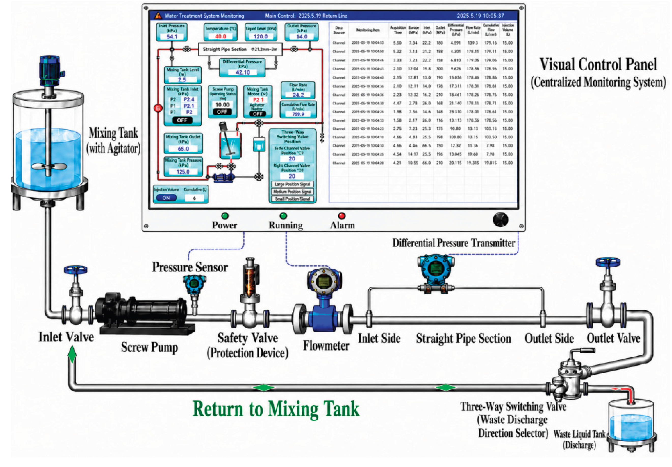
Figure 2.
Schematic test devices.
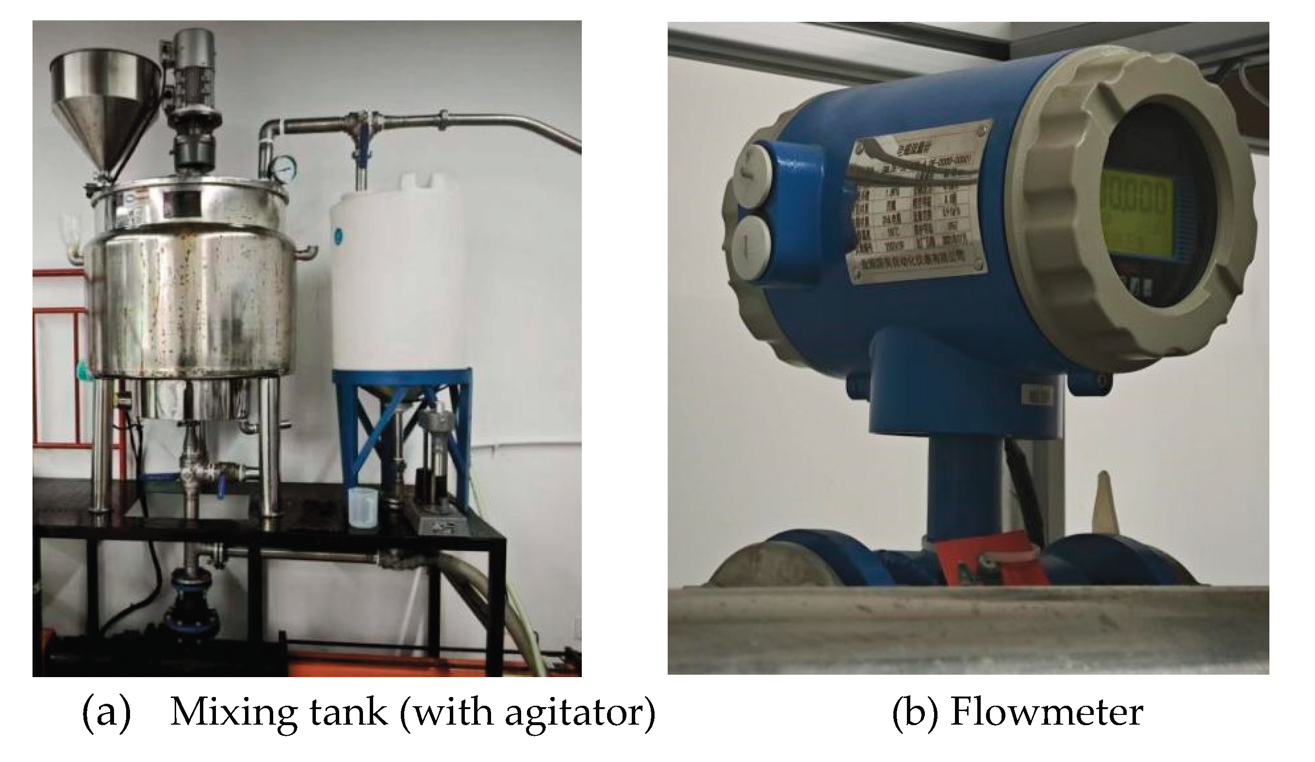
Figure 3.
MARS60 rotary rheometer and its supporting control system.
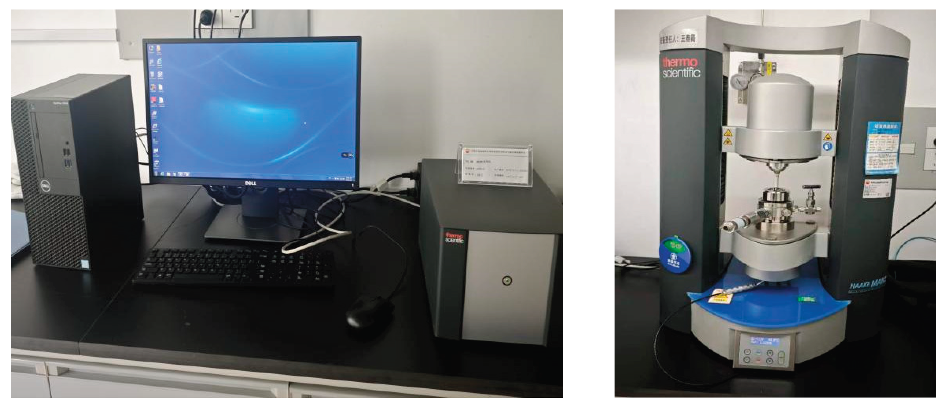
Figure 4.
Schematic computational domain.
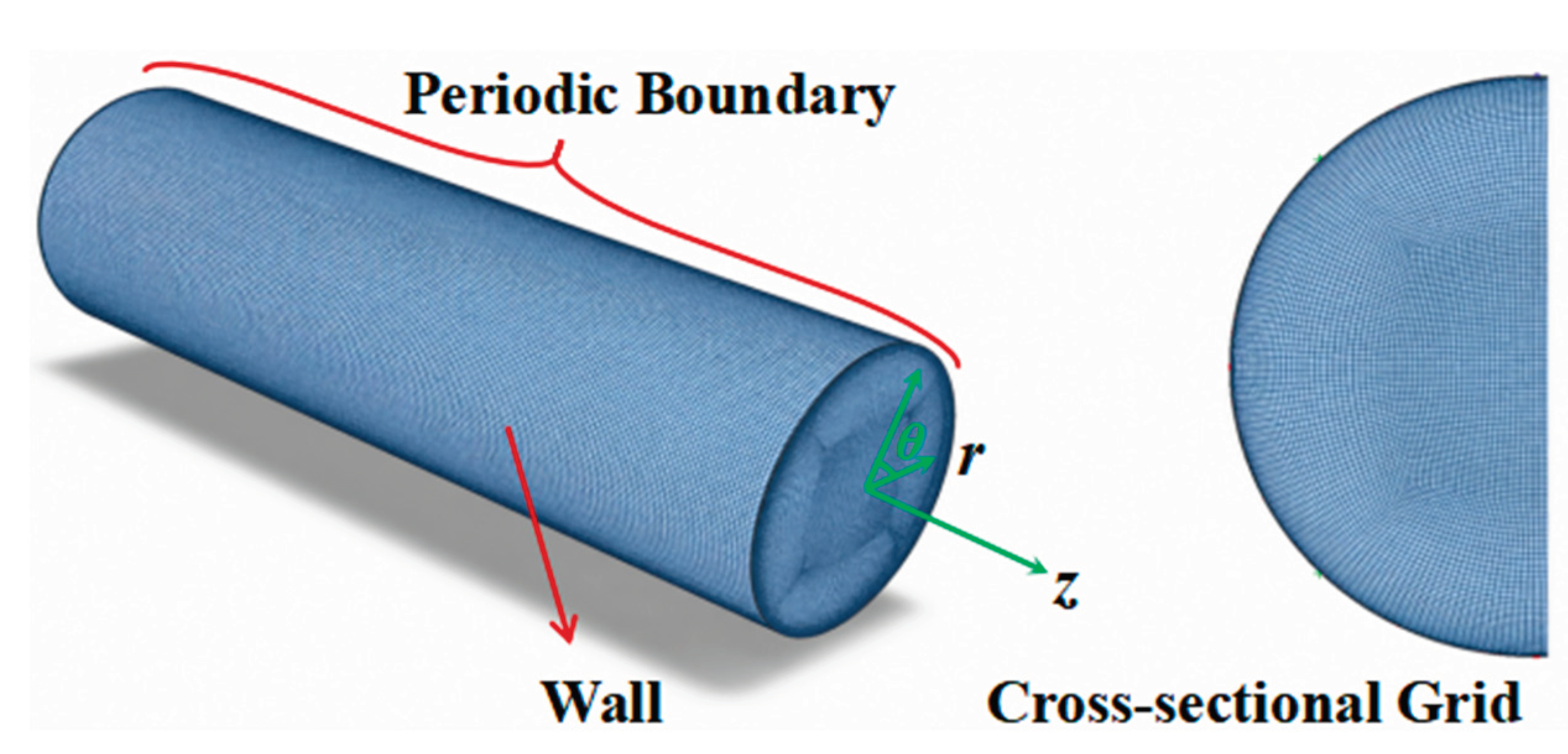
Figure 5.
Comparison between the averaged velocity along the wall normal and DNS results [48].
Figure 5.
Comparison between the averaged velocity along the wall normal and DNS results [48].
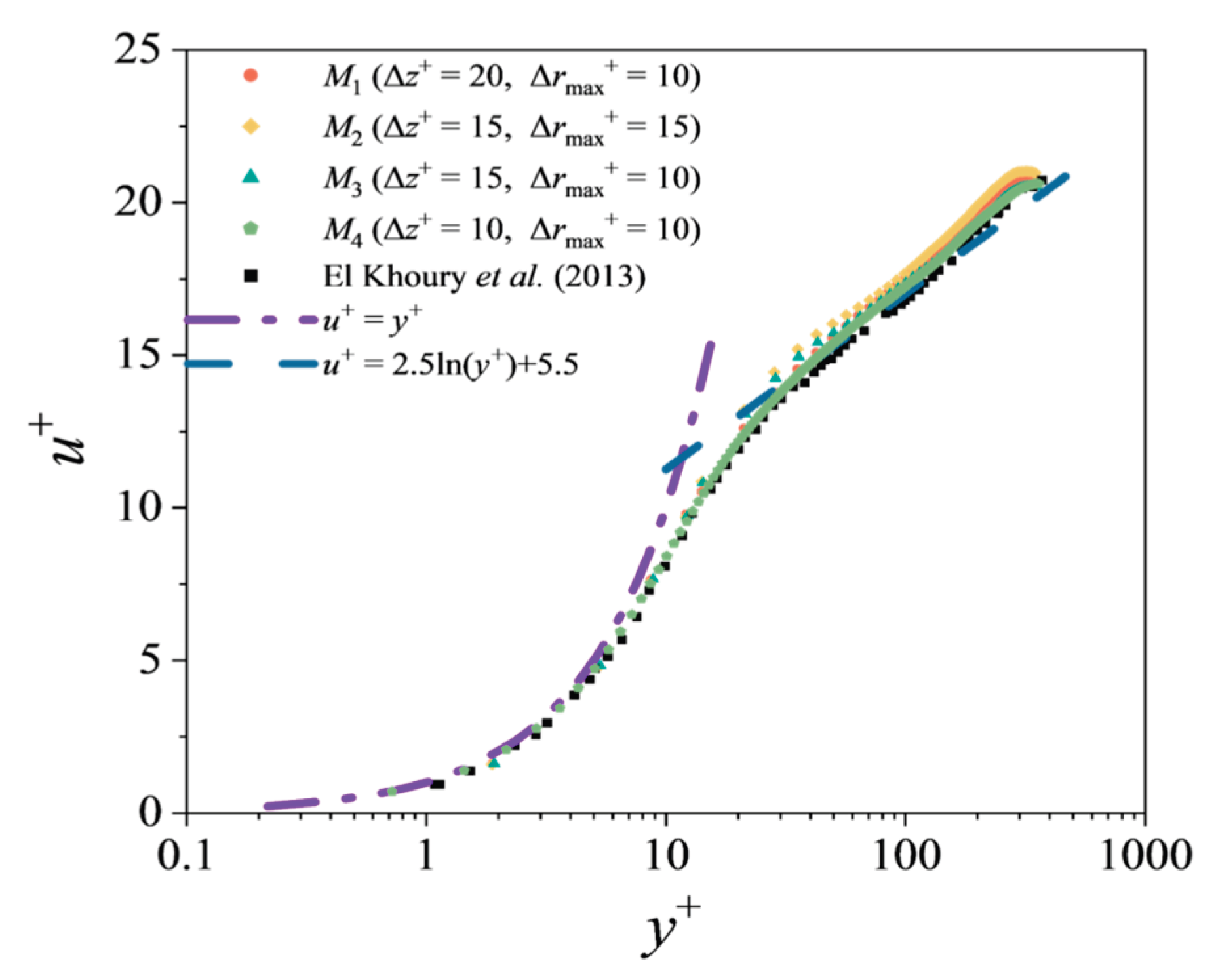
Figure 6.
Comparison of frictional drag between numerical results and experimental results of pipes with diameters of 42 mm and 82 mm [47].
Figure 6.
Comparison of frictional drag between numerical results and experimental results of pipes with diameters of 42 mm and 82 mm [47].
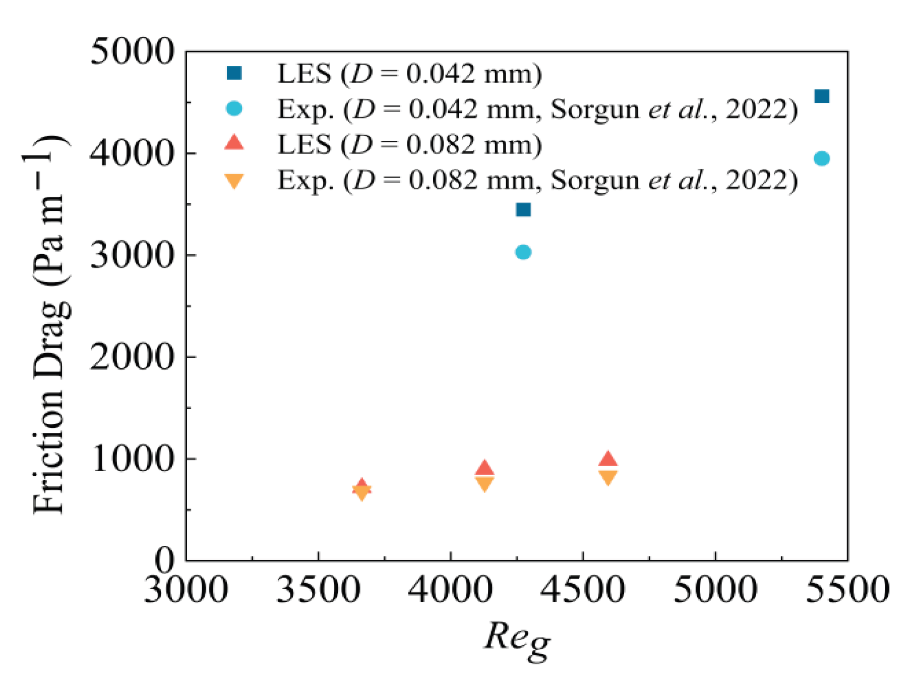
Figure 7.
Comparison of dimensionless Reynolds stress urms+ and vrms+ under various flow conditions and DNS result [48].
Figure 7.
Comparison of dimensionless Reynolds stress urms+ and vrms+ under various flow conditions and DNS result [48].
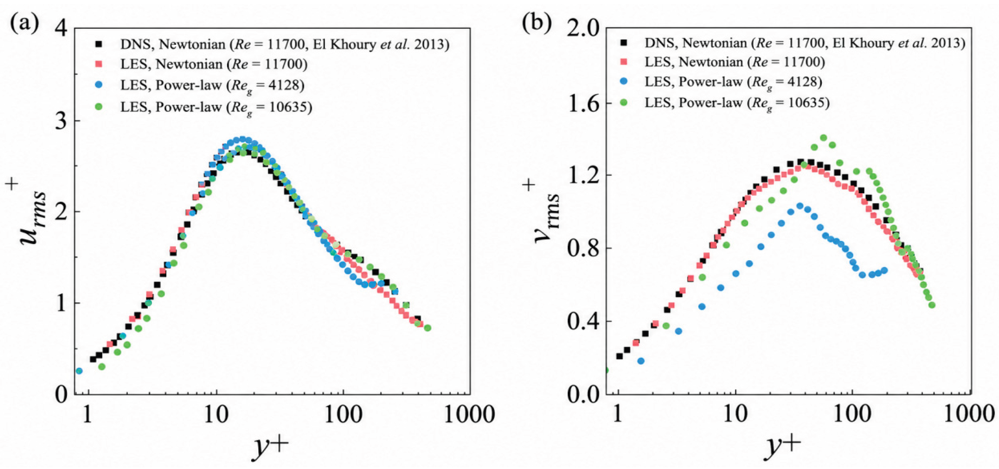
Figure 8.
Variation of (a) pressure drop and (b) DR of PAM solutions with various molecular weights and flow rate.
Figure 8.
Variation of (a) pressure drop and (b) DR of PAM solutions with various molecular weights and flow rate.
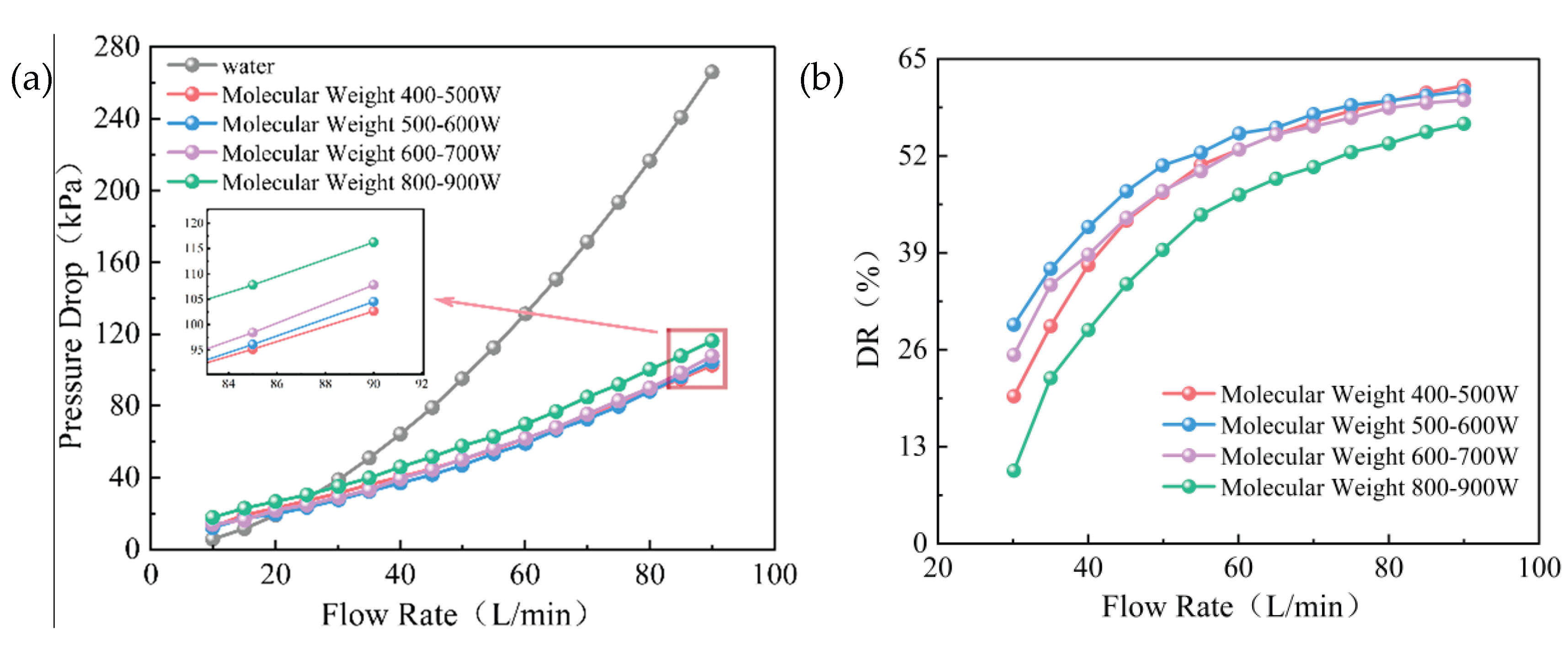
Figure 9.
Variation of (a) pressure drop and (b) DR of PAM solutions with different zero-shear viscosity with flow rate.
Figure 9.
Variation of (a) pressure drop and (b) DR of PAM solutions with different zero-shear viscosity with flow rate.
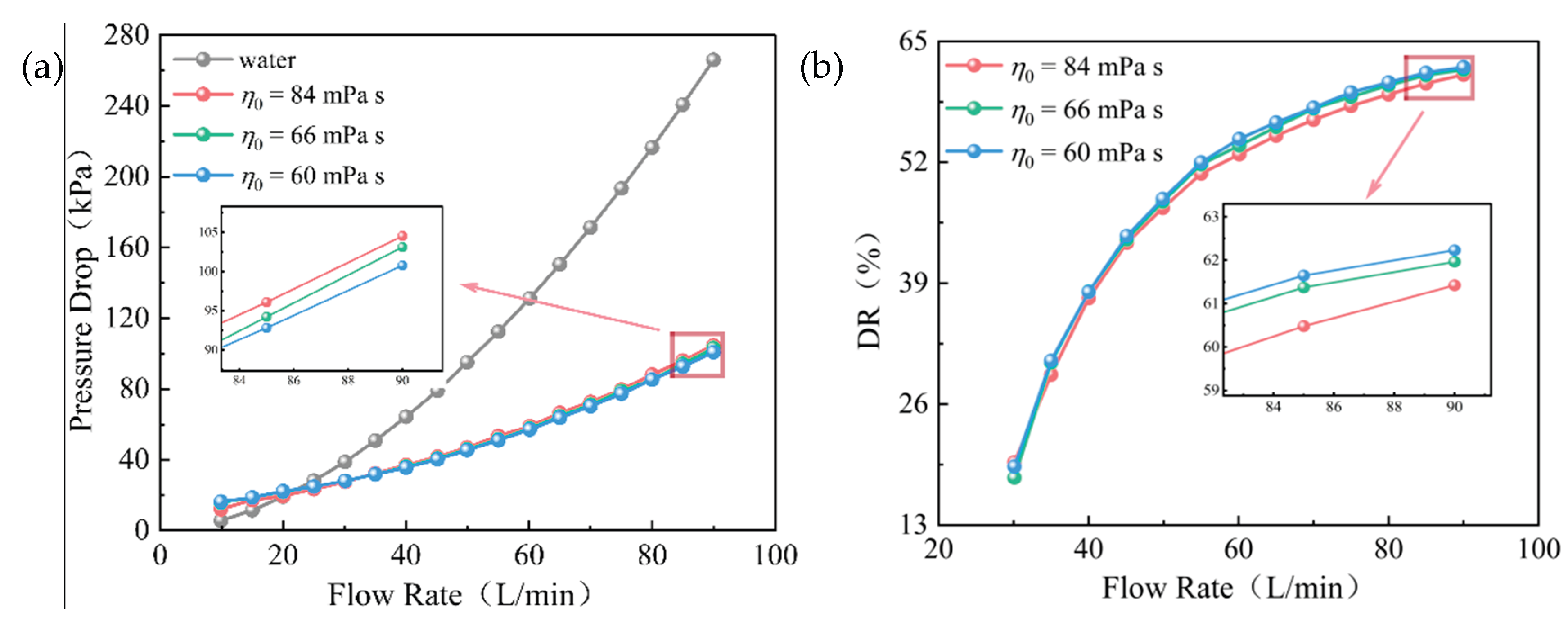
Figure 10.
Variation of (a) frictional pressure drop and (b) DR of various fracturing fluid formulations with flow rate.
Figure 10.
Variation of (a) frictional pressure drop and (b) DR of various fracturing fluid formulations with flow rate.
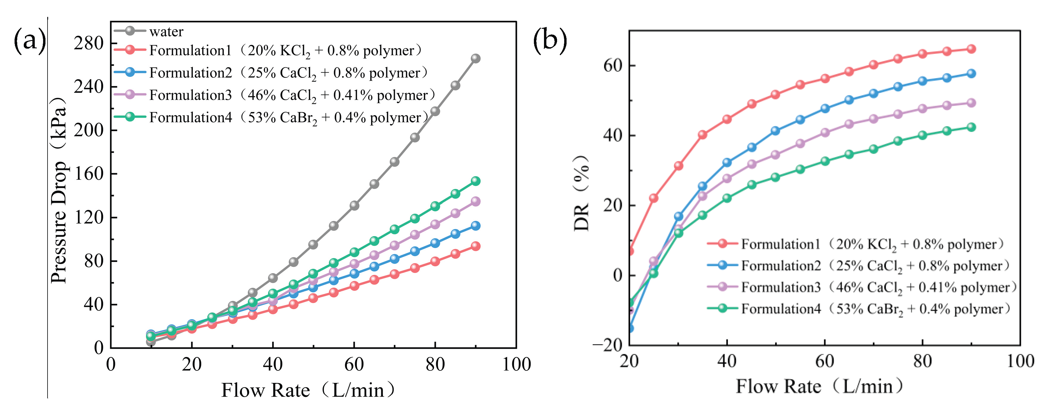
Figure 11.
Variation of apparent viscosity of PAM samples with shear rate.
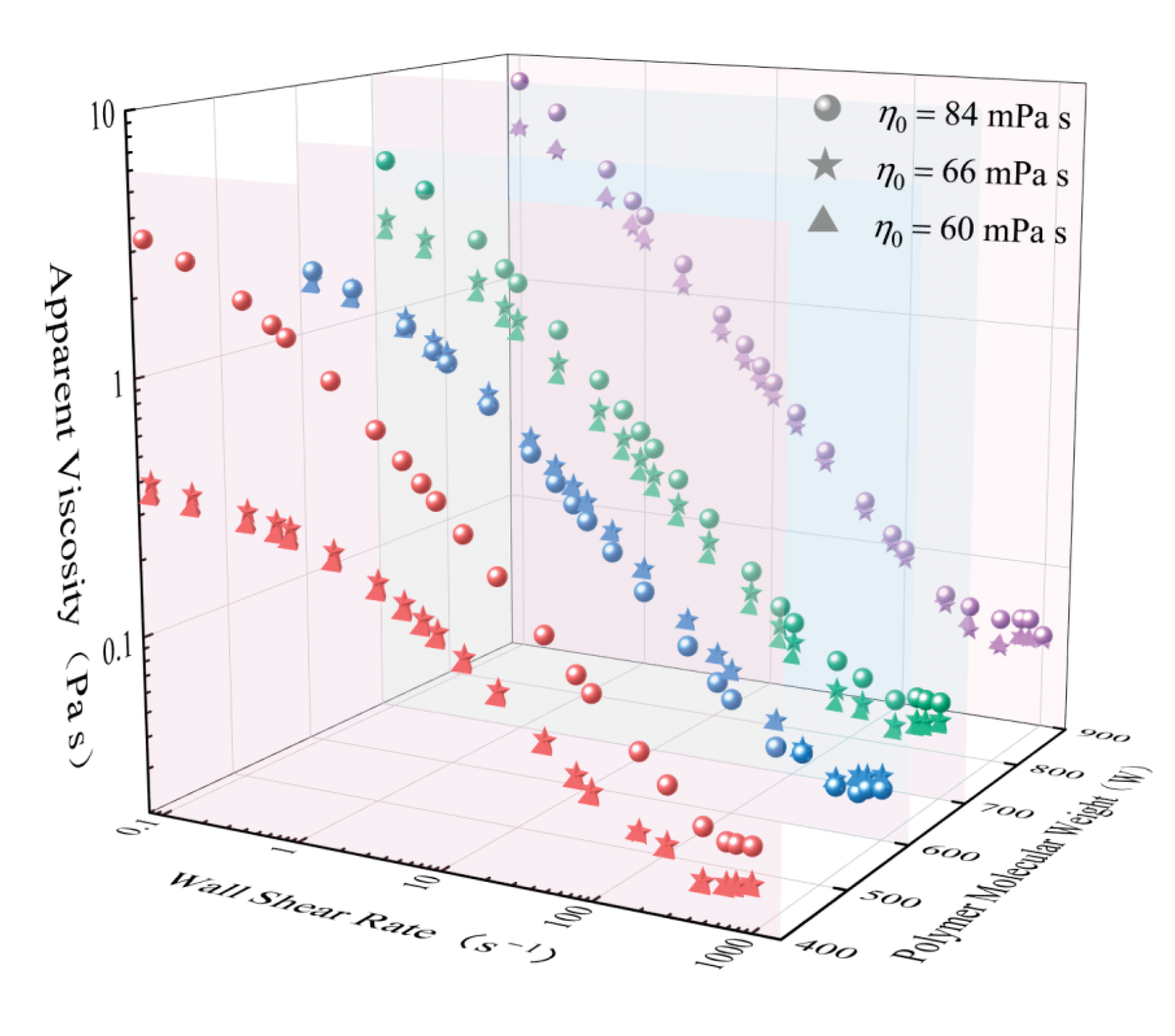
Figure 12.
Rheological behaviors of weighted fracturing fluids and F-1 fluid [47].
Figure 12.
Rheological behaviors of weighted fracturing fluids and F-1 fluid [47].
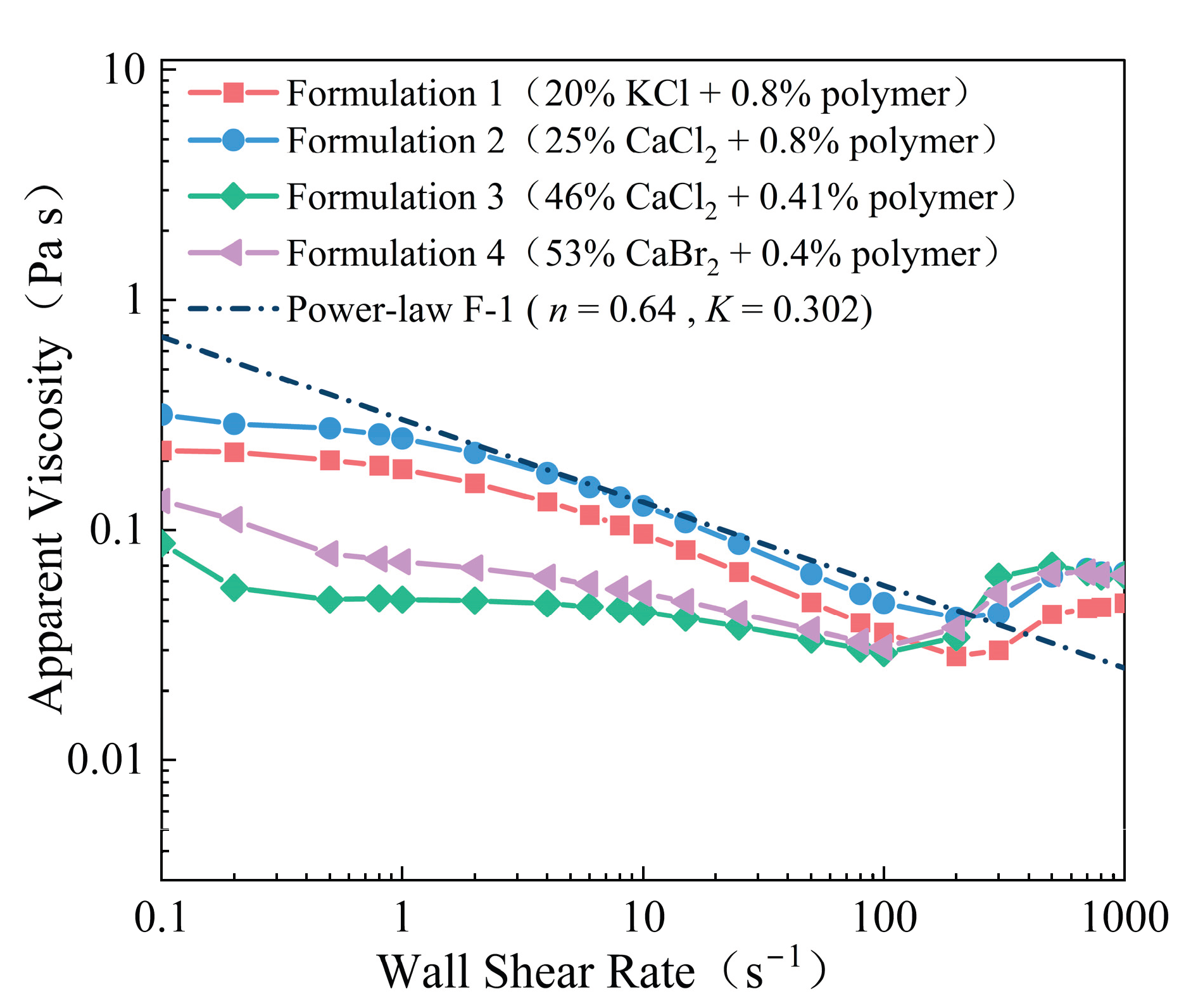
Figure 13.
Average axial velocities for different (a) densities, (b) pipe diameters, (c) K, and (d) n.
Figure 13.
Average axial velocities for different (a) densities, (b) pipe diameters, (c) K, and (d) n.
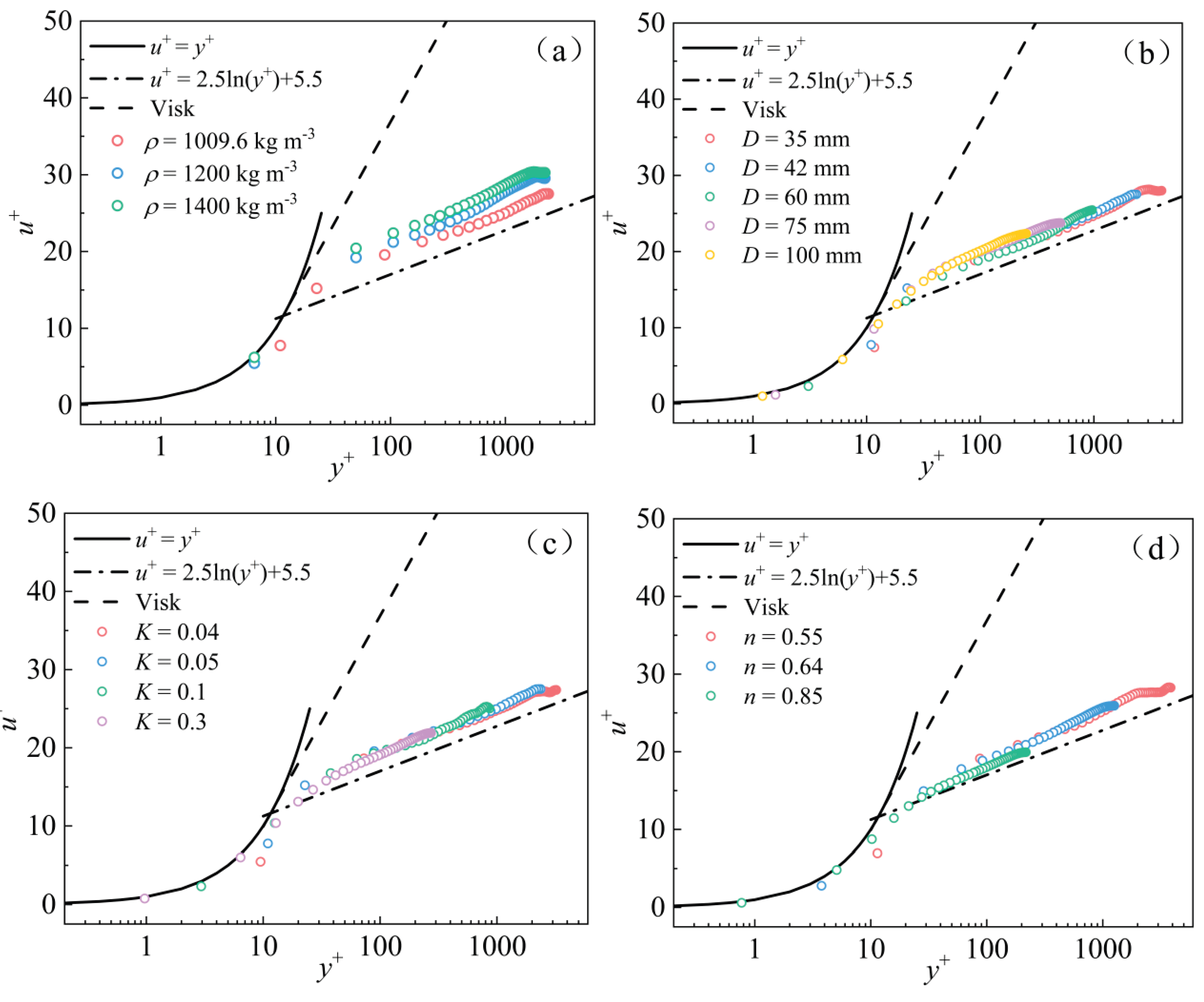
Figure 14.
Velocity contour near the wall at x = -0.0209 m at (a) n = 0.85 and (b) n = 0.55.
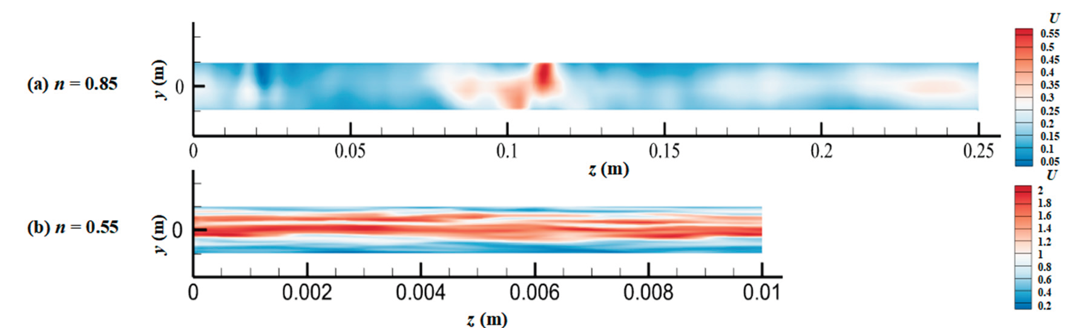
Figure 15.
Q criterion isosurfaces colored by velocity values at (a) n = 0.85 and (b) n = 0.55.
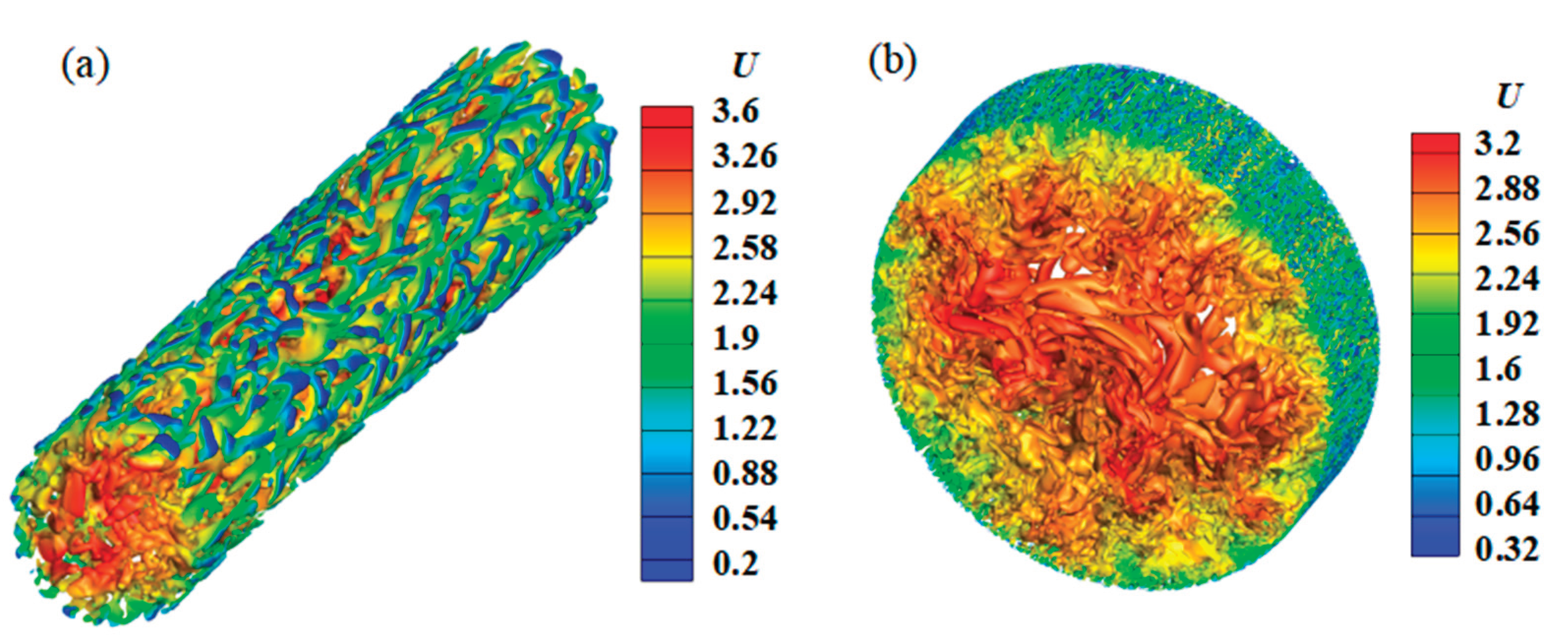
Figure 16.
Cross-sectional vorticity distribution at (a) n = 0.85 and (b) n = 0.55.
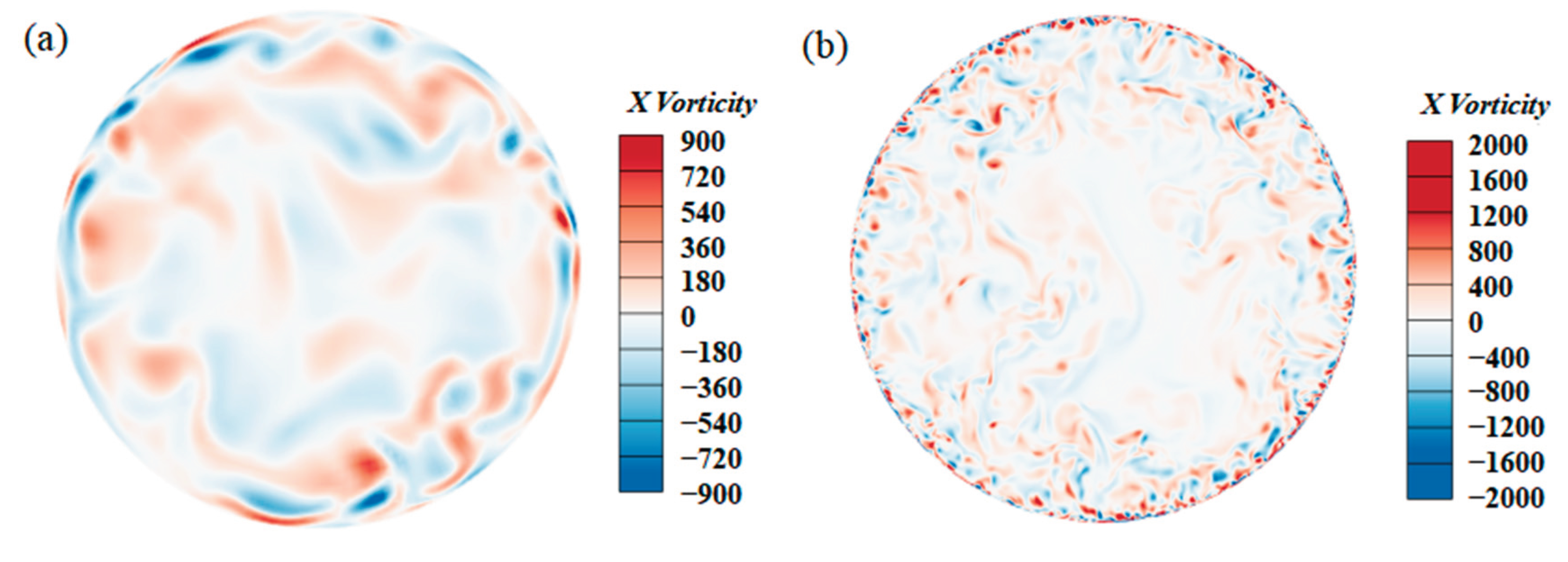
Figure 17.
Comparison between predicted and actual friction factors.
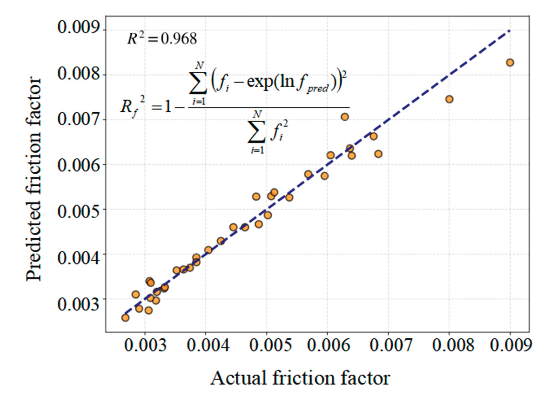
Figure 18.
Sensitivity degree of each parameter to frictional drag.
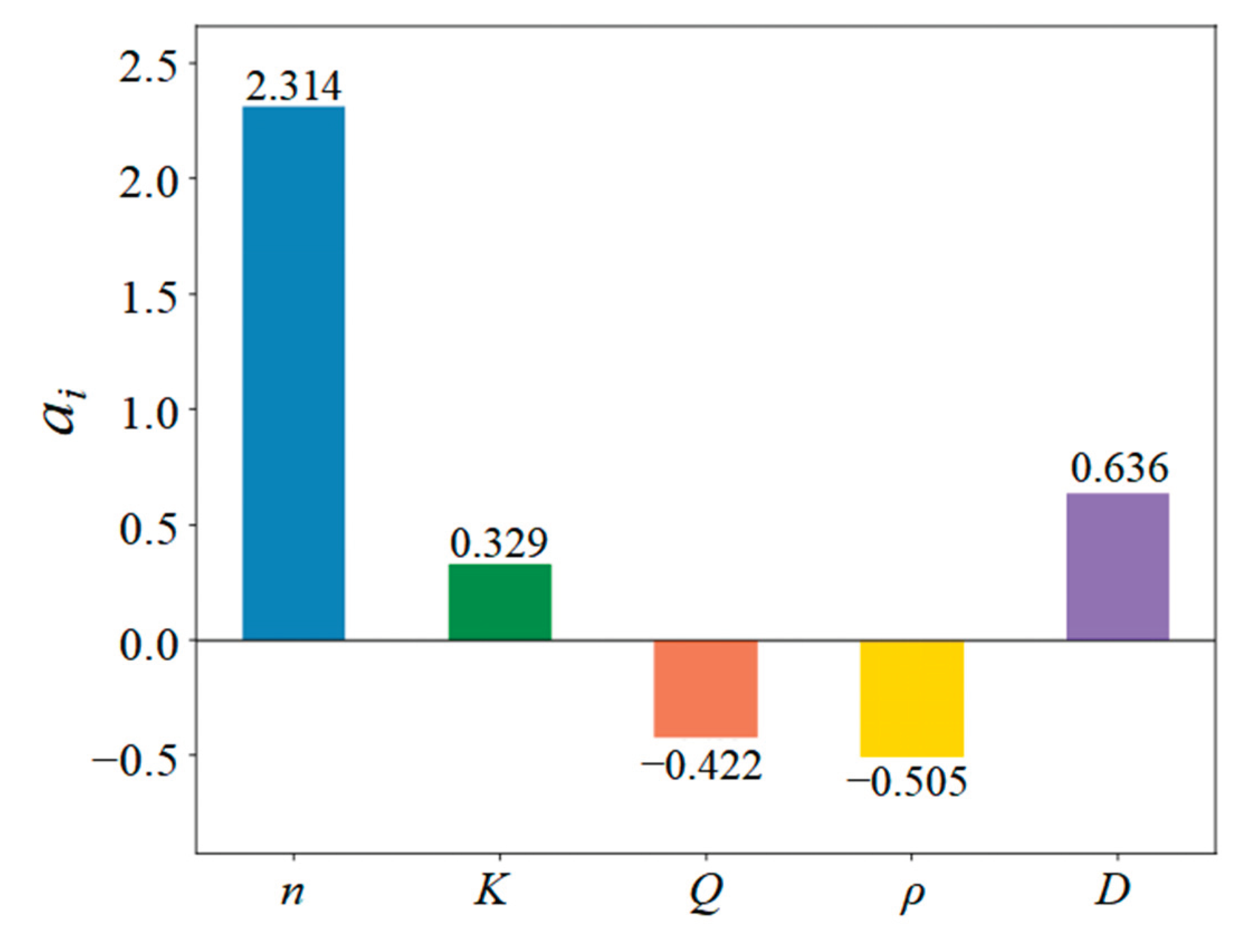
Figure 19.
Variation of friction factor f for four base cases with parameter changing by 1δ, 3δ and 5δ.
Figure 19.
Variation of friction factor f for four base cases with parameter changing by 1δ, 3δ and 5δ.
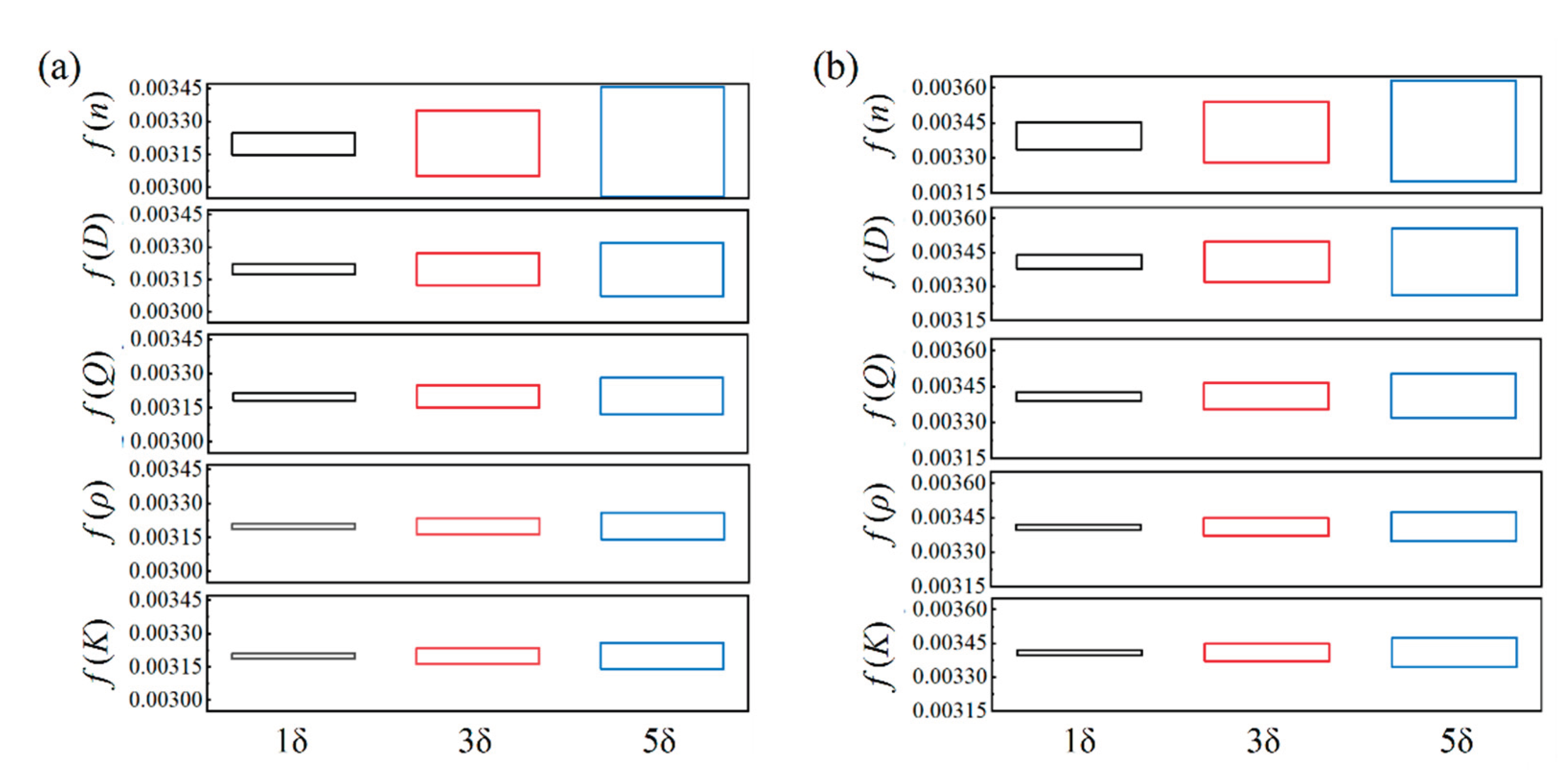
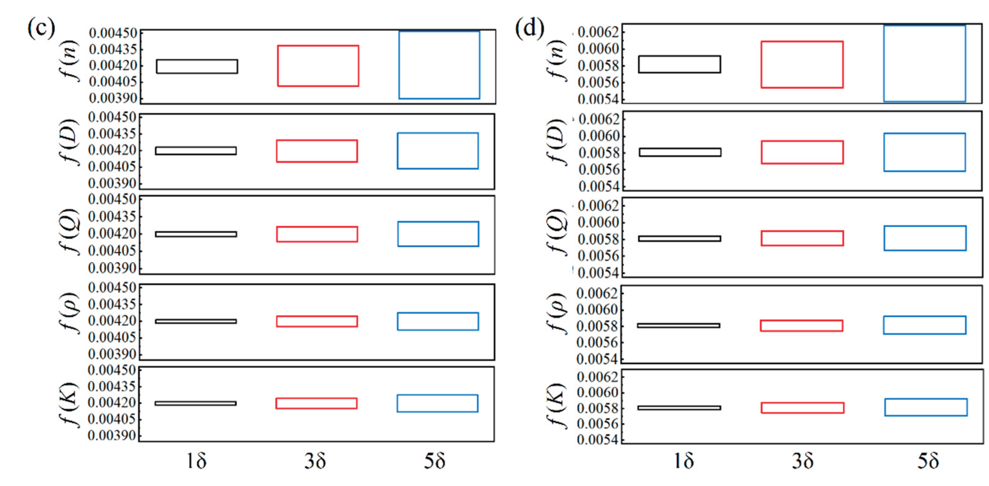
Figure 20.
Sensitivity degree of each parameter to frictional drag.
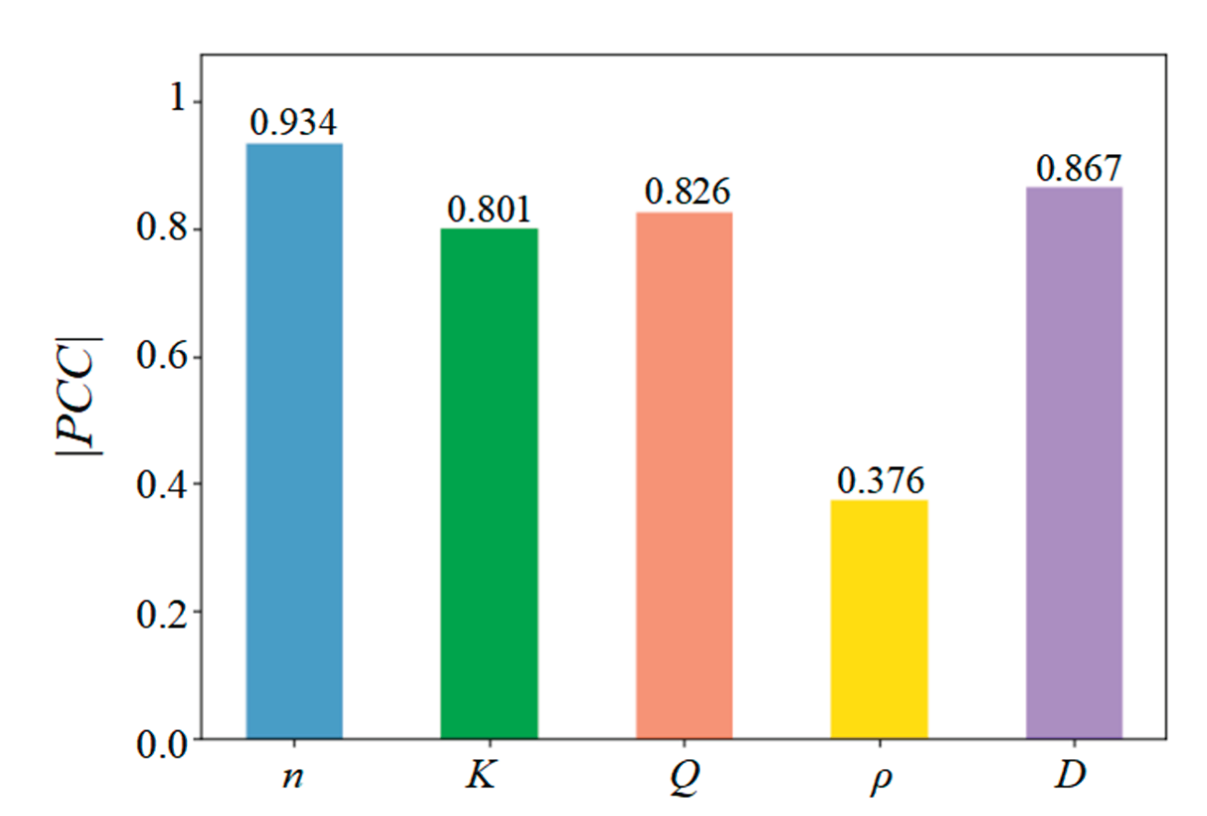

Table 1.
Fracturing fluid formulations.
| Fracturing fluid system | Formulation | Density (kg/m3) | Zero-shear viscosity (mPa·s) |
| PAM solution | Fresh water +0.5% PAM | 1000 | 60–84 |
| KCl-weighted fracturing fluid | Fresh water + 20% KCl + 0.8% polymer + 0.5% temperature stabilizer + 0.5% cleanup additive + 0.5% demulsifier | 1150 | 30.5 |
| CaCl2-weighted fracturing fluid | Fresh water + 25% CaCl2 + 0.8% polymer + 0.1% cosolvent | 1150 | 42 |
| CaCl2-weighted fracturing fluid | Fresh water + 46% CaCl2 + 0.411% polymer + 0.1% cosolvent | 1350 | 34.5 |
| CaBr2-weighted fracturing fluid | Fresh water + 53% CaBr2 + 0.4% polymer + 0.1% cosolvent | 1500 | 30 |
Table 2.
Data of the selected four base cases.
| Base case | ρ0 ( kg m-3) | K0 | n0 | q0 (L min-1) | D0(m) |
| (a) | 1009.6 | 0.04 | 0.64 | 320 | 0.042 |
| (b) | 1009.6 | 0.05 | 0.55 | 220 | 0.042 |
| (c) | 1009.6 | 0.05 | 0.64 | 220 | 0.042 |
| (d) | 1009.6 | 0.2 | 0.64 | 320 | 0.042 |
Disclaimer/Publisher’s Note: The statements, opinions and data contained in all publications are solely those of the individual author(s) and contributor(s) and not of MDPI and/or the editor(s). MDPI and/or the editor(s) disclaim responsibility for any injury to people or property resulting from any ideas, methods, instructions or products referred to in the content. |
© 2026 by the authors. Licensee MDPI, Basel, Switzerland. This article is an open access article distributed under the terms and conditions of the Creative Commons Attribution (CC BY) license.
Copyright: This open access article is published under a Creative Commons CC BY 4.0 license, which permit the free download, distribution, and reuse, provided that the author and preprint are cited in any reuse.