

Submitted:
03 August 2026
Posted:
04 August 2026
You are already at the latest version
Abstract
We simulate the propagation of a single photon propagating within a modal group, traversing through a multimode optical fiber in the presence of mode coupling. We illustrate the propagation graphically on a group of higher order Poincare spheres. The spheres display the propagation of the light within the modal group including polarization in time and in distance as the transmission proceeds. Thus, the amplitudes and the relative phases within the group can be visualized throughout the transmission, which is novel and very useful to understand the propagation. At the fiber output we show how to recover the input of a classical state using the simulated propagation information displayed on such multiple spheres. Once a classical - modal path is established from end to end, one can transmit quantum states, for example a spatial – time binned QKD (quantum key distribution) code. A quantum state follows this classical path. This can include binary or qudit information. Accessing a photon output state is important for many quantum network applications including quantum key distribution, routing and entanglement swapping. In addition, one can use other modal groups within the same fiber to multiplex other quantum channels. Further, one can multiplex within a modal group using principal modes, a more complicated communication method. Using the spheres, this situation is also discussed. Applications include higher dimensional quantum communications, quantum cryptography, and quantum networks. It is important to point out that in today’s commercial quantum communications systems, the quantum states are single photon states but not entangled. This includes both discrete and continuous variable quantum key distribution systems. In this report we are also looking at single photon systems but not entangled, unless stated otherwise.
Keywords:
single photon transmission
; multimode fiber
; quantum key distribution
; higher order Poincare sphere
1. Introduction
Quantum communications and in particular quantum key distribution, QKD, research is of significant worldwide interest. This is occurring due to increased interest in modular quantum computing [1] and in secure communications based on quantum physics, [2,3,4,5]. Quantum technology is mostly based on the processing of qubits [6], the quantum state which has a probability amplitude in being in one of 2 positions, states. Qudits are quantum states that can be detected in one of ‘d’ states. There are advantages to processing quantum information with qudits rather than qubits, but the added implementation complexity is often not understood. Research on this topic is now an important subject for quantum information technology.
Within quantum communications, the transmission of quantum information using advanced states such as W states and GHZ states [7,8] is of importance and current interest. A key advantage is that one can send more quantum information per photon, and it enables more resilient quantum keys [9]. In this report we investigate theoretically and through modeling the possibility of transmitting ‘d’ level quantum states through multimode optical fiber. As an application, we consider transmitting a 4-mode OAM (orbital angular momentum)—polarization quantum state through fiber in the presence of mode coupling. This is like transmitting a polarization—based qubit through single mode fiber, under the presence of mode coupling, but is somewhat more complex. In the single mode fiber case, one recovers the input polarizations states using polarization controllers, first by establishing a path using classical light. Now with the system link stabilized, the qubit can be transmitted and measured. The polarization controllers need to be monitored and adjusted, using classical light on the order of minutes. In the OAM—polarization modal group case, a more complex quantum state results at the fiber output. Using the quantum field distribution, which we display on a group of Higher Order Quantum Spheres, one can coherently combine both the spatial modal and polarization fields to recover the input state. One can now use quantum use time binning to transfer quantum information. Time binning [10] is often used today to transfer a quantum key through single mode fiber links. In analogy to the BB84 protocol using linear or circular polarization for launching and detection, here one uses an early or late time or, analogous to circular polarization, early—late time combinations with a phase relationship. Recently ‘d’ level time binning including entanglement [11] has been demonstrated using single mode fiber.
The technology and the photonic components required for the implementation of higher dimensional quantum communications is currently being helped by advancements in spatial—mode division multiplexing [12] for the purposes of increasing the capacity of classical optical communications by increasing the number of channels. The growth of classical communications continues to grow at an exceptional rate. And it is now being greatly enhanced by the communications demands resulting from the rapid hardware—commercial implementations of Artificial Intelligence, A I.
Interest in commercial—classical communications using few mode fiber and mode division multiplexing is growing. Current commercial deployments incorporate MIMO [13,14] to deal with the mode coupling that occurs during signal propagation. These systems require significant power to implement digital system processing and are not therefore suitable for quantum communications. Principal Mode transmission, however, can be used to overcome the deleterious effects of the mode coupling [15,16,17,18].
Apart from mode division multiplexing and principal mode transmission, higher dimensional quantum communications are of interest in that one can transmit more information per photon [9] and for some quantum networks [19]. So, it is an objective of this communication to focus on the transmission of single photons through higher dimensional space, but without the increased complexity of mode division multiplexing and principal modes. The coherent properties of the photon are important as one needs to recover the input photon state to retain the quantum information or if one wants to implement entanglement swapping. Entanglement swapping is of interest for long distance communication [20] and for quantum networks. For entanglement swapping, the photons undergoing the swapping need to be identical in polarization, spectrally, and in spatial mode. If they are not identical, modal transformations are required before the swapping. In the single mode fiber case, polarization controllers are used to regain the initial polarization state. This is required due to the polarization coupling that occurs in the transmission. In the multimode—higher dimensional situation, we need a similar method to regain the initial quantum state, spatial—polarization mode. We investigate this by simulating the transmission of a single photon transmitting through a 4-transmission medium. With an end-to-end channel established, one can us time binning, including ‘d’ level time binning, to transmit quantum information. We consider a 2 polarization—2 spatial mode such as an LP11 mode in an optical fiber. This numerical simulation is independent of the fiber index profile. The profile can be for example a step index or parabolic profile [21], we are only concerned with the coupling within a modal group, for example the LP11 mode.
In Section 2, Modal propagation in Optical Fiber, we write the mode coupling propagation equations for a photon transmitting through a 4 mode (2 spatial modes times 2 polarization modes) channel within a fiber. Such modes occur within an LPνµ mode of a multimode fiber [21]. In order to track and display the propagation, we propose using a group of Poincaré spheres [22]. We track the propagation along an input sphere and then coupling to other spheres (adjacent modes) as the propagation progresses.
We can isolate an LPνµ mode in an optical fiber when the number of spatial—polarization modes are on the order of 16 modes, and the modal groups are on the order of 6 [23]. This is because the modes in an optical fiber separate into modal groups [21,24] that are nearly degenerate and coupling between modal groups is minimal because the axial perturbations to enable this coupling is on the order of millimeters, which is very unlikely. Coupling within a modal group is however likely because axial perturbations to enable this coupling is on the order of meters and more, which is likely. A modal group typically includes 2 polarizations modes and 2 spatial modes for ν > 0, and 2 polarization modes and 1 spatial mode for ν = 0. For this reason we focus our attention on the propagation of a photon within a 4-mode optical group.
Mode coupling in optical fiber is a vast subject [24,25,26,27,28,29]. Gloge [26] showed that mode coupling among modes can be described with a diffusion are equation. This is especially appropriate for fibers with many modes, because the simulation of power flow among these modes is of importance and the diffusion equation works well here. However, in many cases and in single photon propagation, the amplitude and the phase of the propagating fields are important and the power equations eliminates the phase information. In fact, the evolution of the phase values and the field amplitudes as the photon propagates within an optical modal group are key to understanding single photon propagation in an optical fiber.
Here we present a novel approach to the visualization of both the amplitude and the phase of a single photon as it propagates within an optical modal group of a multimode fiber. We display these values on multiple Higher Order Poincare spheres. We limit the propagation of the light to within an LPνµ 4 modes and there is no coupling between the other modal groups. This sets the boundary to 4 modes and coupling to other modal groups is zero, a very reasonable assumption.
In Section 3, Mode Coupling, Mode Coherence and Field Recombination at the Fiber Output, we discuss how to use the calculated or experimentally determined classical field information to coherently combine the polarized—modal information to recover the input state. Once this is established, a time bin quantum state can be transmitted and measured at the output. This recovery is necessary because any mode coupling distorts the coherency of the quantum state.
In Section 4, Multiple—Higher Order Poincare Spheres and the Geometry of the Quantum State, we discuss the relationship of the higher order Poincare sphere to the geometry of the quantum state and the implications of the SU(N) geometry and to principal modes.
In Section 5, Discussion, Multiple Photons, we discuss and show graphically the simultaneous propagation of multiple photon states
In Section 6, Outlook, we discuss the current research status as it relates to the implementation of higher dimensional quantum communications.
2. Modal Propagation in Optical Fiber
Propagation of light in optical fiber is well described by the scaler wave equation [21], when the index difference between core and clad is on the order of a few percent. The axial solution is a propagating wave in z and is a function of the radius r, and the radial, µ, and azimuthal, ν, numbers as well as the index distribution with radius. The scaler wave equation is written as:
The scalar wave equation can be solved using an Eigen solution method [21]. Here a set of basis functions are used to obtain the wave functions which are superpositions of these basis functions. Typically, Laguerre Gauss functions are used as the basis functions and the solutions are characterized as LP, linearly polarized modes. These solutions are functions of a radial function (µ ) and an azimuthal function (ν). For ν not equal to 0, they are also characterized as orbital angular momentum modes. For circular cores, the LPνµ modes are separable in their radial, azimuthal and axial components and can be written as:
Spatial—higher dimensional quantum communications [9] intends to use these spatial distributions as channels for communication with distance.
As mentioned in a multimode fiber we can restrict single photon propagation to within an LPνµ polarization—spatial mode. Since cross coupling between LPνµ modes can be limited we simulate the propagation of the single photon within the 4 modes of this polarization—spatial mode. So we have 4 modes, 2 polarization and 2 spatial. The +- signs represent alignment with the x, y axis
So, we have 4 possibilities, and an unentangled W quantum state can be written as [7]
In theory, one can use any LPνµ mode to transmit a W(4) state, but LP(ν=+-1, µ =1,2,3) are most easily isolated in a fiber (21).
Mode coupling within these LP modes is common and expected due to stresses and strains on the fiber due to the deployment. The mode coupling equations describing this coupling are described by Matera and Someda for example. [32]. They describe the polarization mode coupling in optical fiber. Consider now the propagation of the 4 modes within an the LPνµ mode described above. Like Matera and Someda the mode coupling equations are:
In Equation (4a), βis the propagation constant of the LP mode, the k are the mode coupling coefficients. In eq 4b, S is a stress optic coefficient [33]. These mode coupling coefficients represent the effects of fiber twisting, bending and core deformation and these effects are well described by Ulrich and Simon [33]. In this simulation, we use their coupling coefficients for the situation of twists, because twisting is a most effective way to implement mode coupling.
Here τ is the twist rate per unit length, n is the core index, and p44 is one of the photo elastic coefficients and is related to p11 (.116 in silica) and p12 (-.26 in silica) as
Here, we use a twist rate of 2 twists per meter. It is important to note that these coupling parameters drift in time on the order of minutes depending on the fiber deployment and environment. Therefore, they can be considered constant for transmissions of hundreds of kilometers and therefore the systems transmission matrix can be fixed. But the detection system needs to be capable of adjusting with this drift and a new transmission matrix exists defined on this order in time. This is the situation in today’s QKD systems as the the polarization controllers in the single mode case are adjusted on this time scale.
Numerically solving Equations (4)–(7), we use python code 3.11.4 and matplotlib.pyplot to plot the 3 dimensional sphere information. The step size was 1. Millimeter for the optical path length—step size and lowering the step size to .1 mm did not make a difference in the calculated propagation paths. The response to calculate the paths and display a sphere was less than a second. We chose a beat length of 1 and.5 meters, but the calculations scale with linearly length We chose these values because typically 1 meter is chosen to simulate polarization mode dispersion [34]. However, in today’s commercial fibers, these beat lengths are more than 10 times these values.
Light propagating and coupling between two polarizations in time can be displayed on a Poincaré sphere (22). Born and Wolf show how to use the amplitudes and phase of the two components to plot the light’s position on the sphere as the propagation continues
3. Mode Coupling, Mode Coherence and Field Recombination at Fiber Output
With 4 modes, there are 6 combinations of the fields of i and j. So, we can plot 6 spheres simultaneously as light propagates and then couples among the 4 modes. So, for the 4 modes, we can take 2 modes at a time and plot a sphere for each. So the spheres will be of: (E1,E2; E1,E3; E1,E4); and (E2,E3,E2,E4) and (E3,E4). If we input light into |1>|1> the propagation combines mode |1,1> with |1,-1>. This is the combination of OAM1 and polarization +1 combining with OAM1 with and polarization -1. The light propagates and couples with the parameters of Equation (4) under the coupling equations above with a cross coupling birefringence (beat length) of 1 meter between the 2 OAM modes two different polarizations and a beat length of one-half meter between an OAM mode of the same polarizations. The beat lengths of the 2 polarizations in commercial optical fibers vary considerably on the order of 1 to more than 10 meters. In this simulation we choose these meter lengths as mentioned above, but the results of the simulations scale with the transmission length vs. the beat lengths.
In this case as the light couples from the input OAM mode of a specific polarization to the other polarization, spheres, the radius of the sphere is unity, but then as it begins to couple to the other possibilities, the radius of the tracking shrinks, and other sphere tracking begins to appear and grow in radius. We plot below the 6 spheres as the light propagates up to 100 meters. We use Python 3 d graphics to plot the spheres, Figure 1A–C. At the output of the fiber, the light from each sphere can be coherently combined to a position on a defined sphere. With applications in mind, we discuss below how to combine these fields at the fiber output, enabling one to transfer a quantum state. In these figures, the black curves outline the surface of the sphere, and the green curve shows the trajectories of the light for the modes mentioned. The blue dot shows the position at which the light is input, always onto mode 1.
Consider the first 3 spheres above marked, M1, M2: M1, M3; and M1, M4. These spheres display the phase difference between the two fields Mi and Mj, as well as their amplitudes. Using the spheres in Figure 1A, one can relate the modal fields in M2, M3, and M4 to those of M1. So, M1 can be chosen as the reference to which the other fields relate. By rotating the spatial fields at the output to align and or the polarizations to align, one can coherently combine the fields by shifting one field with respect to the other by the phase difference. The phase difference is proportional to S3. The phase at the polar Z axis maximum is π/2. Experimentally, these phase differences can be implemented with for example a Cailabs—C multiple beam phase controller. The polarizations can be rotated with a half wave plate and the fields can be rotated with flat optics for example [35]
Amplitude and phase corrections need to be on the order of minutes and more for polarization of 2 polarization modes [36,37] for example. There is not much data on the requirements for spatial mode correction, but it is reasonable to assume these correction times will be similar. The Calilab devices exhibit insertion losses on the order of 1 to 3 dB. The fiber losses in long distance quantum link of .15 dB/km, so accounting for this loss, corrected quantum bits are received on the order of seconds [38].
4. Multiple—Higher Order Poincare Spheres and the Geometry of the Quantum State
The W state of Equation (3) can be used to transfer a qudit with more information per photon than that of a qubit [9]. As mentioned, we can do this using an LPνµ mode in an optical fiber. Due to mode coupling during propagation, the photon in an initial OAM state and polarization state can have a probability amplitude of being in the other OAM mode and or the other polarization as was shown in the Figure 1. A sphere represents the relative amplitude and phase of 2 electric fields. In the typical Poincaré sphere, this is the relation of 2 polarizations, but also in a higher order Poincare sphere, characterizing orbital angular momentum modes [39]. In our case we have spheres combining 2 fields of a propagating OAM mode, which can have field combinations of a spatial field with a polarization and another spatial field with a different polarization.
The photon output therefore has a probability amplitude of being in each of the 4 positions with a specific value. Again, in our situation the 4 positions are composed of 2 polarizations and 2 spatial modes. In single mode optical fiber, the quantum state can be graphically displayed on the Poincare sphere. In higher dimensional quantum communications, the quantum states need to be displayed on a higher dimensional sphere, something we can’t do in a 3-dimensional world. So, we propose to use a group of spheres to display the quantum information. The Poincare sphere is used to display fiber polarization—propagation information in single mode fiber and this is an SU(2) quantum geometry. Any 2-dimensional quantum state can be displayed on this sphere. Also, any quantum state in this situation can be mathematically described as a specific sum of the Pauli matrices, which represents the quantum geometry of these states. Likewise, the geometry of an N dimensional quantum state is an SU(N) geometry [18]. Also, any state in an SU(N) geometry can be mathematically represented as a specific sum of the generalized Gell Mann N2 -1 generators quantified with the generalized Gell Mann matrices. Interestingly using these generators, principal states can be determined enabling the possibility of spatial division multiplexing in the presence of mode coupling [18,41,42]. This is also the case with single mode fiber where one can polarization multiplex without cross talk using principal states based on polarization and determined using the Pauli spin matrices. These principal states are launched using a combination of polarization modes mathematically described with the Pauli spin matrices [42]. In the case of multimode fiber, mathematically the generalized Gell Mann matrices are used to generate the launch conditions. Again, this is because any quantum state in an N dimensional geometry can be described mathematically using the generalized Gell Mann matrices and then cross talk free states are the principal states, solved with an eigen value matrix. The Gell Mann matrices are important as they relate to determining principal modes, because all states in these systems can be described using these matrices. This is why the principal states can be determined by using them.
Most often however, in today’s commercial quantum communication QKD systems, multiplexing is not utilized, and principal states are not required. However, because polarization mode coupling occurs during transmission, polarization controllers are required to coherently combine the transmitted state to the intended polarization state output.
5. Discussion: Multiple Photons
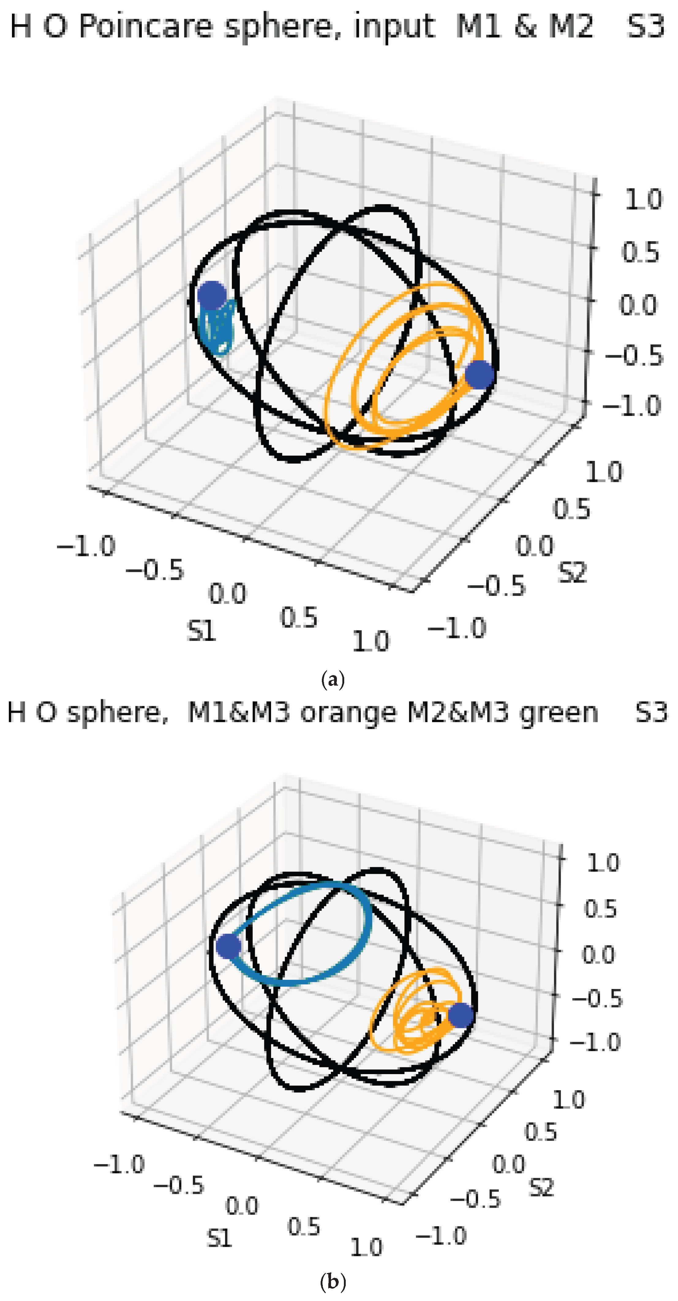
Regarding further the geometry of the quantum state, we can also plot two separate input photons on the spheres. Figure 2 below shows the trajectories of two photons on a sphere. One photon is launched onto mode 1, while a second photon is launched onto mode 2. The trajectories of photon 1, launched onto the fiber oscillate more between modes 1 and mode 2 than does photon 2. This is because photon 2 couples mode easily to mode 3 than photon 1. And this results because the difference in propagation constants between modes 1 and 3 is larger than this difference between modes 2 and 3. The differences between propagation constants significantly affect the amount of coupling [24]. The propagation constants for these simulations are chosen as below, with an index difference of each mode differing from the core index of 1.5. These index differences correspond to the beat lengths between the modes of a meter and one half meter.
6. Outlook
Quantum communications is in an early state of implementation. Applications are mostly in cryptography; quantum key distribution using single mode optical fiber and point to point systems. Higher dimensional quantum communications is in the earlier research stage. Advantages include the possibility of quantum communicating with more information per photon and multiplexing. Also, higher dimensional quantum communications offer the possibility of using these dimensions to enable new possibilities in network routing [19]. In addition, new enhanced encryption methods and materials are evolving that can be applicable here [35]. This is expected to be a very fruitful area of research and eventually lead to commercial implementation. In network routing, the routing is based on multiparticle entanglement. Multiple particle entanglement can be based on wavelength, polarization and spatial mode. Longer term, one could expect all three of these possibilities to be utilized. Regarding scalability, the LP modes can be used to isolate uncoupled groups and the modes in a selected LP mode can be used for the transmission. For example, we can consider the LP modes in a ring core fiber [35]. The LP01 and LP02 modes can be used separately to transmit 2 polarization modes. The LP11, LP21, LP31, LP12, and LP31 modes each can be used to transmit 4 mode quantum states. Quantum memories will also play a role as the memory will be used to store the photons for entanglement swapping. The number of wavelengths available in a quantum network, will most likely be less than those in a classical network, due to the more complex requirements of these memories. Thus, the need for additional entanglement parameters such as space and polarization. It is also possible to include time as an entanglement parameter, but using time in this way will slow done the network. The OAM hardware components including OAM entanglement swapping [43] continue to undergo worldwide research. In fact, some of these components have been commercially available for more than 10 years , albeit at a low level.
References
- Edd Gent, IEEE Spectrum, 27 Feb, 2025.
- Bennett, C. H.& Broussard, G., (1984), Quantum Cryptography, Public key distribution and key tossing. Proceeding of IEEE International Conference on Computers, Systems and Signal Processing, 175–179.
- B. Korzh, et. al., Provably secure and practical quantum key distribution over 307 km of optical fiber, arXiv:1407.7427v1 [quant-ph] 28 July 2014.
- Lo, Hoi-Kwong, Curty, M., and Qi, B., Measurement-Device-Independent Quantum Key Distribution, Phys., Rev., Lett, 108, 10.1103, 2012.
- A. Boaron, et. al., Secure Quantum Key Distribution over 421 km of optical fiber, Phys. Rev. Lett.,121, 190502, 2018. [CrossRef]
- Nielsen, M., Chuang, I., Quantum Computation and Quantum Information, Cambridge, 2000.
- Prevedal, R., Experimental All-)optical One-Way Quantum Computing, Sudwestdeutcher Verlag, 2009.
- Cozzolino, D., et. al., High dimensional quantum communications: benefits, progress, and future challenges, Adv. Quantum Technol 2019, 2, 190038. [CrossRef]
- Mirhosseini, M et. al., High-D Quantum Technol 2019, 2, 190038 High-Dimensional Quantum Cryptography with Twisted Light, New Journal of Physics, 17, 033033, (2015). [CrossRef]
- Boaron, A, et. al., Simple 2.5 GHz time—bin quantum key distribution, Appl. Phys. Lett. 112, 171108, 2018.
- Yu, H., et. al., Quantum key distribution implemented with d-level time bin entangled photons, nature communications, 2025, 16:171. [CrossRef]
- Richardson, D., Fini, J. and Nelson, L. Space Division Multiplexing in Optical Fibers, Nature Photonics, 2013, 7, 354,.
- Van Uden, Okonkwo, C., et. al., MIMO equalization with adaptive step size for few mode fiber transmission systems, Optics Express, 22, 1, 119–126, 2013. [CrossRef]
- Karadimitrakis, A., et. al., IWCS 2014 Barcelona, Spain, 2014, pgs 966–070,.
- Fan, S., Kahn, M., Principal modes in multimode fiber, VDM publications: Saarbrucken, Germany, 2010.
- Carpenter, J., Benjamin, J., Eggleton, J, Comparison of principal modes and spatial eigenmodes in multimode fibre, Lasers & Photonics Reviews, 11, 1, 1600259, 2016.
- Xiong, W., determining principal modes in a multimode fiber using the mode dependent signal method, JOSA, B, 32, 143–149, 2015. . al., Principal modes in multimode fibers: exploring the crossover from weak to strong mode coupling, arXiv:1609.025 [phys.optics], 2016.
- Milione, G., Nolan, D., Alfano, R., Determining principal nodes in multimode fiber, using mode delay method, JOSA B, 32, 143–149, 2015.
- Gu, X, Chen, L., Zeilinger, A., and Krenn, M., Quantum experiments and graphs III: high-dimensional and multi-particle entanglement, arXiv:1812.095582v2 [quant-ph] 2 April 2019.
- Sangouard, N., Simon, C., de Riedmatten, H., Gisin, N., Quantum repeaters based on atomic ensembles and linear optics, arXiv: 0906.2699v2 [quant-ph] Jun, 2009.
- Black, R., and Gagnon, Optical Waveguide Modes, McGraw Hill, 2010.
- Born, M. and Wolf, E., Principal of Optics, Pergamon Press, 1959 Ge, D., A 6-LP-mode ultralow-modal-crosstalk double-ring-core FMF for weakly-couples MDM transmission, Optics Communications, 451 (2019) 97–103, 2019.
- Ge, D., A 6-LP-mode ultralow-modal-crosstalk double-ring-core FMF for weakly-couples MDM transmission, Optics Communications, 451 (2019) 97–103, 2019. [CrossRef]
- Vassallo, C. Optical Waveguide Concepts, Elsevier, 1992.
- Marcuse, D., Theory of Dielectric Optical Waveguides, Academic Press, 1991.
- Gloge, D., Optical power flow in multimode fibers, Bell Syst. Tech J. 51, 1767–1783 (1973). [CrossRef]
- Olshansky R. and Nolan, D., Mode-dependent attenuation of optical fibers: excess loss, Appl. Opt. 15, 1045-1047 (1976). [CrossRef]
- Savovic, S., et. al., Temperature dependence of mode coupling in low-NA plastic optical fibers, J. of Lightwave Technology, 33, 1, 2015. [CrossRef]
- Birri, A., et. al., Thermally induced bend loss of optical fiber, IEEE Sensors Journal, 18(5) 2018 6181–6187. [CrossRef]
- Meunier J., Pigeon, J., Massot, J., A general approach to the numerical determination of modal propagation, 2025. n constants of optical fibers, Opt. Quantum Electron, 1981 13, 71-83. [CrossRef]
- Lavery, M., et. al. Refractive elements for the measurements of the orbital angular momentum of a single photon, Opt. Express 2012, 20, 2110–2115. [CrossRef]
- Matera, F. and Someda, C., Random birefringence and polarization dispersion in long single—mode optical fibers, in Anisotropic and nonlinear optical waveguides, Elsevier, 1992.
- Ulrich, R. and Simon, A, Polarization optics of twisted single-mode fiber, Appl. Opt., 1979, 18, 2241–2251. [CrossRef]
- Li, M., Nolan, D., Fiber spin profiles designs for producing fibers with low polarization mode dispersion. Optics Letters, 23, 1659–1661, 1998. [CrossRef]
- Yao, O, et. al., Flat optical rotator enabled by conformal mapping, Laser and photonics news, 12 Nov.
- Honjo, ., et. al., Long distance entanglement based quantum key distribution over optical fiber, Optics Express, 16, 19118–19126, 2008.
- Nadaalong, T., Automatic compensation of polarization drift in an optical fiber, Theis, Maximilians-Universitat, Munchen, 2018.
- Korzh, B. et. al., Provably secure and practical quantum key distribution over 307bkm of optical fibre, arXiv:1407v1 [quant-ph] 28 July, 2014.
- Milione, M. Szul, H., Nolan, D., and Alfano, R., Higher order Poincare sphere and the angular momentum of light, Phys. Rev., Lett, 107, 053601, 2011.
- D. Nolan, Higher-Dimensional communications using multimode fibers and compact components to enable a set of communicating channels, Optics, 2024, 5 330–341. [CrossRef]
- D. Nolan, Simulating Higher-Dimensional quantum communications using principal modes, Optics, 2025, 6 24. [CrossRef]
- Gordon, J. and Kogelnik, H. PMD fundamentals: polarization mode dispersion in optical fibers, Proc Natl. Acad. Sci., USA 2000, 97, 4541-4550. [CrossRef]
- Erhard, M., Mehul, M. and Zeilinger, A quantum router for high-dimensional entanglement, IOP Science, Quantum Science and Technology, 2, 014001, 2017.
- Lopez –Bastida, Classical encryption demonstration with BB84 protocol—inspired coherent states using reduced graphene oxide., Quantum rep 2025(3), 35.
- Graffitti, F. et. al., Hyperentanglement in structured quantum light, Physical Review Research 2, 043350 (2020). [CrossRef]
Figure 1.
A, HOM for modes 1 & 2, 1&3 and 1 &4. Light is input onto mode 1 and the sphere position is indicated in blue. The coupling proceeds according to the green trajectory, and the sphere is outlined in black. B, HOM for modes 2 & 3, and 2 & 4 Light is input onto mode 1, position indicated in blue on the sphere. The trajectory proceeds according to the green line and the surface of the sphere is indicated in black. C, HOM for modes 3 & 4 Light is input onto mode 1, position indicated in blue on the sphere. The trajectory proceeds according to the green line and the surface of the sphere is indicated in black.
Figure 1.
A, HOM for modes 1 & 2, 1&3 and 1 &4. Light is input onto mode 1 and the sphere position is indicated in blue. The coupling proceeds according to the green trajectory, and the sphere is outlined in black. B, HOM for modes 2 & 3, and 2 & 4 Light is input onto mode 1, position indicated in blue on the sphere. The trajectory proceeds according to the green line and the surface of the sphere is indicated in black. C, HOM for modes 3 & 4 Light is input onto mode 1, position indicated in blue on the sphere. The trajectory proceeds according to the green line and the surface of the sphere is indicated in black.
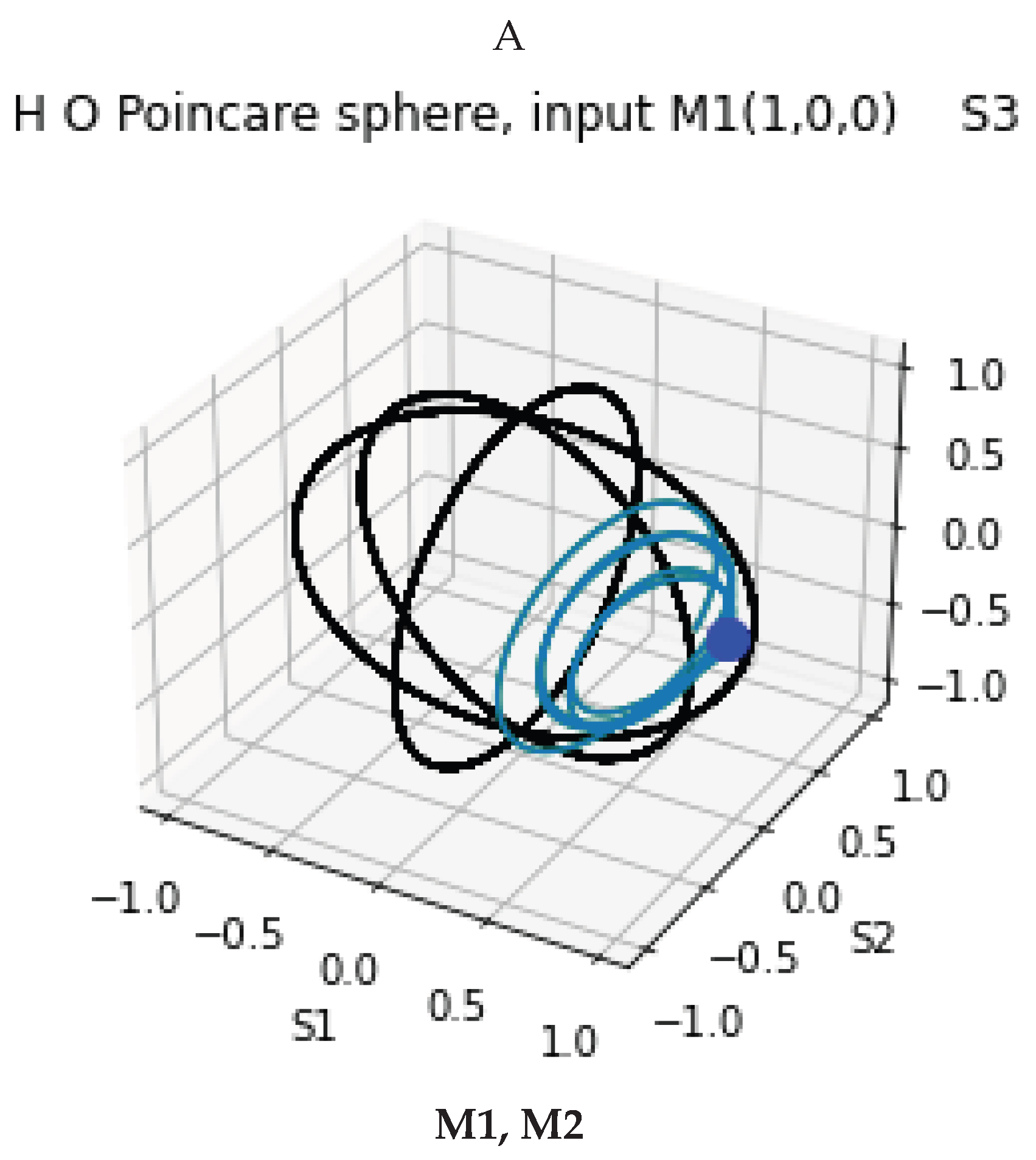
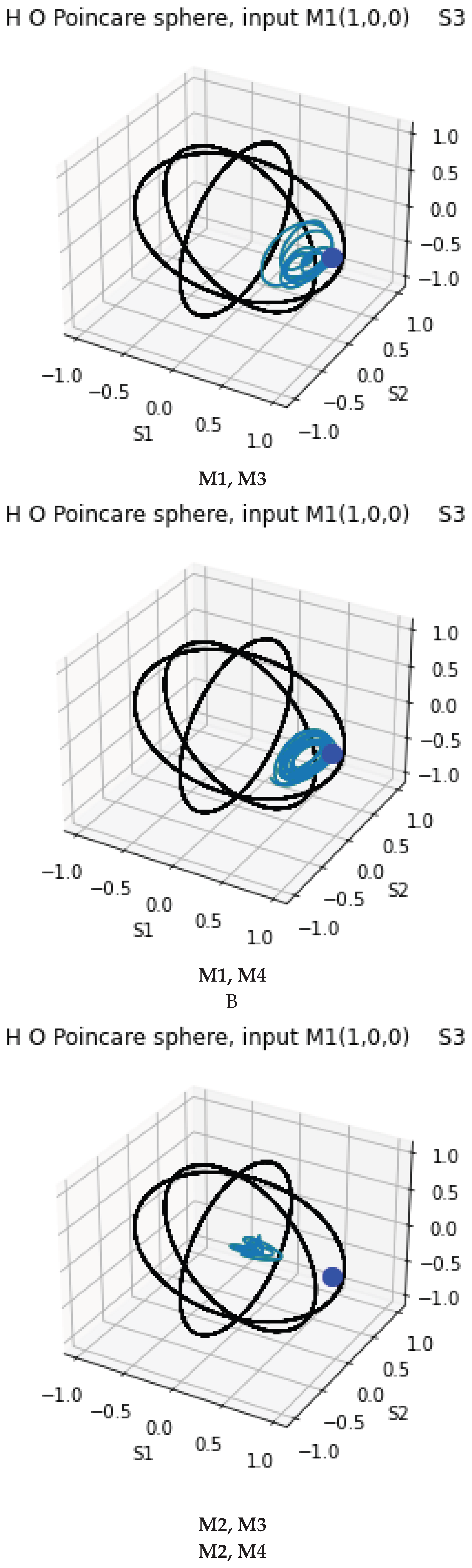
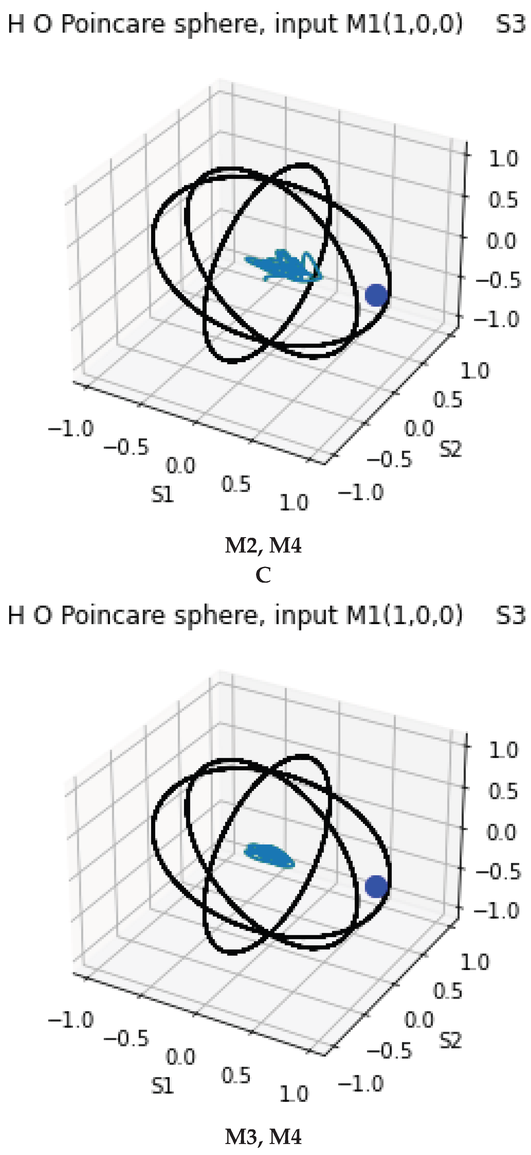
Figure 2.
a, two photons launched. Light is input onto mode 1, position indicated in blue on the sphere. The trajectory proceeds according to the orange line. The modes considered are mode 1 and mode 2. Separately, light is launched onto mode 2, position indicated in blue on the sphere. The trajectory proceeds according to the green light. The surface of the sphere is indicated in black. b, two photons launched. Light is input onto mode 1, position indicated in blue on the sphere. The trajectory proceeds according to the orange line. The modes considered are mode 1 and mode 3. and the coupling is between modes 2 and mode 3. Separately, light is launched onto mode 2, position indicated in blue on the sphere. The trajectory proceeds according to the green light. The surface of the sphere is indicated in black. In order to eliminate interference of these 2 photons at a detector, one needs to use principal mode transmission as described above, since with more than 1 single photon or channel we are multiplexing.
Figure 2.
a, two photons launched. Light is input onto mode 1, position indicated in blue on the sphere. The trajectory proceeds according to the orange line. The modes considered are mode 1 and mode 2. Separately, light is launched onto mode 2, position indicated in blue on the sphere. The trajectory proceeds according to the green light. The surface of the sphere is indicated in black. b, two photons launched. Light is input onto mode 1, position indicated in blue on the sphere. The trajectory proceeds according to the orange line. The modes considered are mode 1 and mode 3. and the coupling is between modes 2 and mode 3. Separately, light is launched onto mode 2, position indicated in blue on the sphere. The trajectory proceeds according to the green light. The surface of the sphere is indicated in black. In order to eliminate interference of these 2 photons at a detector, one needs to use principal mode transmission as described above, since with more than 1 single photon or channel we are multiplexing.
Disclaimer/Publisher’s Note: The statements, opinions and data contained in all publications are solely those of the individual author(s) and contributor(s) and not of MDPI and/or the editor(s). MDPI and/or the editor(s) disclaim responsibility for any injury to people or property resulting from any ideas, methods, instructions or products referred to in the content. |
© 2026 by the authors. Licensee MDPI, Basel, Switzerland. This article is an open access article distributed under the terms and conditions of the Creative Commons Attribution (CC BY) license (http://creativecommons.org/licenses/by/4.0/).
Copyright: This open access article is published under a Creative Commons CC BY 4.0 license, which permit the free download, distribution, and reuse, provided that the author and preprint are cited in any reuse.


