

Submitted:
03 August 2026
Posted:
04 August 2026
You are already at the latest version
Abstract
Artificial intelligence (AI) is increasingly used for tool-wear prediction in computer numerical control (CNC) machining, yet a high average accuracy can conceal systematic failure in the safety-critical high-wear region, where under-prediction makes a worn tool appear healthier than it is. This paper presents a trustworthy multimodal framework that audits, mitigates, and ultimately characterises this bias on the public MATWI dataset. A fusion model combining 512 image features with 84 force, acceleration, and acoustic features attains a strong test mean absolute error (MAE) of 30.9 µm, outperforming image-only (51.4 µm) and sensor-only (68.3 µm) baselines. A signed, stratified bias audit nevertheless reveals a pronounced directional error: the model predicts the healthy region to within 21.3 µm but under-predicts the worn region by approximately 85 µm (worn-region MAE 85.5 µm), with the error deepening monotonically as wear increases. A three-stage mitigation pipeline (data-level resampling, cost-sensitive and relevance-based training, and post-hoc recalibration) reduces the worn-region error by up to 18% but cannot eliminate it, and only at a measurable cost to the well-sampled region. The residual bias is shown to be both model-independent, persisting across six regressor families with a 69–127 µm residual gap, and optimisation-independent, surviving rigorous hyperparameter search and bias-aware loss functions behind an ≈ 85 µm error floor. These results establish the bias as data-intrinsic: it arises from the sparse sampling of the high-wear regime rather than from model or training choices, and the effective remedy lies in balanced, unbiased data collection rather than further algorithmic correction. The contribution is a reusable protocol for distinguishing model-reducible from data-intrinsic bias in safety-critical regression.
Keywords:
trustworthy AI
; tool-wear prediction
; predictive maintenance
; multimodal fusion
; imbalanced regression
; bias mitigation
; target-region fairness
; CNC machining
; data-centric AI
1. Introduction
1.1. Why Trustworthy AI in Manufacturing
Artificial intelligence (AI) and machine learning (ML) are changing how factories operate. Tasks such as predictive maintenance, quality control, and process optimisation are moving from reactive inspection toward data-driven decisions made in advance [1,2,3]. Predictive maintenance is one of the clearest success stories: by predicting the future condition of machines and tools from sensor and image data, AI systems can reduce unplanned downtime, lower scrap, and extend the life of expensive assets [4,5]. However, a gap remains between the high accuracy reported in research papers and the level of confidence needed to use these models on a real shop floor, where a wrong decision can be costly or unsafe [1,6].
This gap is, at its core, a problem of trust. Manufacturing is moving from the automation focus of Industry 4.0 toward the human-centred vision of Industry 5.0. In this newer view, AI is not meant to replace people but to support them — a shift often described as augmentation rather than automation [7,8,9]. An AI model becomes a working partner: it offers a recommendation, and a human operator or engineer decides whether to act on it [9,10]. For this partnership to work, the operator must know when the model can be relied upon and when it should be treated with caution [10]. Trustworthy AI (TAI) has therefore become a key requirement for adoption. It brings together the properties — reliability, robustness, transparency, fairness, and accountability — that allow an AI system to be used safely alongside people [2,6,11].
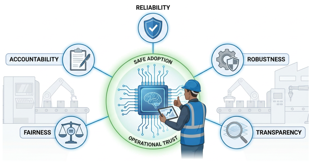
Figure 1.
Trustworthy Artificial Intelligence (TAI) as an enabler of safe AI adoption in manufacturing. The framework highlights five core trustworthiness dimensions: reliability, robustness, transparency, fairness, and accountability. Together, these attributes establish operational trust, support human–AI collaboration, and promote the safe, effective, and responsible deployment of AI systems in industrial environments
Figure 1.
Trustworthy Artificial Intelligence (TAI) as an enabler of safe AI adoption in manufacturing. The framework highlights five core trustworthiness dimensions: reliability, robustness, transparency, fairness, and accountability. Together, these attributes establish operational trust, support human–AI collaboration, and promote the safe, effective, and responsible deployment of AI systems in industrial environments
A high accuracy score does not, by itself, make a model trustworthy. A model can have a low average error and still fail on the small group of cases that matter most for safety. Tool wear prediction in CNC milling, the use case studied in this work, is a clear example. As a cutting tool wears, part quality drops and scrap increases; in the worst case, the tool can fail suddenly and halt production [5,12]. The high-wear region is therefore the most safety-critical part of the prediction range. If a model regularly underestimates wear in this region, it makes a worn tool appear healthier than it is and delays replacement past the safe point. This one-sided error — the systematic underestimation of high-wear cases — is not just a statistical detail; it is a safety-relevant bias that affects the most important failure mode. Building trust in a wear-prediction model therefore means showing not only that it is accurate on average, but also that it is not biased against the cases that matter most.
This study uses the MATWI dataset (Multimodal Automatic Tool Wear Inspection) as its experimental basis [12]. MATWI is a publicly available dataset built from real CNC milling runs. It follows 17 carbide milling inserts from new condition until failure, with around 100 measurements taken across each tool’s life. Each measurement pairs a microscope image of the cutting edge with sensor signals from an accelerometer, a microphone, and a force table [12]. Flank wear, the main wear indicator, is measured on a scale of roughly 0 to 450 m — a range fine enough that a human inspector cannot judge it reliably by eye [12,13]. The dataset also contains other wear types, such as adhesive wear and chipping, and some tools were run on a different workpiece material, which changes the visual appearance of the wear [12]. These properties make MATWI well suited to studying trustworthy wear prediction, but they also introduce the bias risks described next.
1.2. Challenges
Several well-known weaknesses of data-driven models act together to produce exactly the bias described above. They can be grouped into data-centred and model-centred issues.
The main data-centred issue is imbalanced data. In milling datasets, most measurements are taken while the tool is healthy or only lightly worn, while high-wear examples are naturally rare [14]. When a regression model is trained on such skewed data with a standard loss such as mean squared error, training is dominated by the crowded low-wear region. To keep the average error low, the model pulls its high-wear predictions toward the more common middle values, which is the direct cause of the dangerous underestimation noted above [14,15]. The study of this problem — models failing in thinly sampled parts of a continuous target range — is known as deep imbalanced regression [14,16]. A related risk is overfitting: with so few high-wear examples, the model may simply memorise them rather than learn a general pattern, which looks good during training but fails on unseen tools [14].
A second and less obvious issue is spurious correlation, also called shortcut learning. Deep networks often rely on accidental patterns in the data — such as workpiece material or wear type — that happen to align with the wear label, instead of learning the true visual signs of wear [17]. In MATWI this risk is concrete, because some tools were run on a different material and show more adhesive wear with a different appearance [12]. A model may score well when tested under familiar conditions but fail once these accidental patterns are absent, which harms both reliability and fairness [17].
On the model side, the black-box nature of large deep models makes these problems harder to detect. When a model cannot explain its reasoning, an operator cannot easily tell a well-grounded prediction from one based on a shortcut or on guessing in a data-poor region. This works against the calibrated trust that human–AI collaboration depends on [6,11]. Finally, there is a growing concern about reproducibility. Results in ML-based research are often sensitive to training settings, undocumented preprocessing, and data leakage, which can make them appear stronger than they are and difficult to repeat [18,19]. In a safety-critical setting, a result that cannot be reproduced cannot be trusted.
Standard engineering practice does not fully resolve these problems. Overall scores such as RMSE or average performance across the whole wear range and therefore hide poor performance in the high-wear region [14]. Common fixes, such as bin-weighted training or class-weighted classification, are usually applied on their own and are rarely paired with a clear analysis of where the bias comes from or an evaluation that uses fairness metrics. What is missing is a structured approach that treats bias as a central concern: identifying its sources, reducing it at several stages of the modelling process, and measuring the resulting trade-off between accuracy and fairness.
Intended Deployment Scenario
The system studied in this paper is designed to support a specific operational workflow in CNC milling, illustrated in Figure 4. After each milling pass, the cutting-edge image and the process-sensor recording from that pass are acquired automatically. The multimodal model processes both and produces three outputs: (1) a continuous wear estimate with a 90% prediction interval, which gives the operator a quantitative health indicator for the tool; (2) a binary inspection flag that fires when the predicted wear type suggests the tool has moved beyond normal flank wear into adhesive or combined wear requiring closer examination; and (3) the prediction interval itself, which quantifies the model’s uncertainty and signals when the estimate should be treated with caution.
The human operator receives all three outputs and makes the final replacement decision. The model is therefore not autonomous: it is a decision-support tool that reduces the information burden on the operator by converting raw image and sensor data into actionable indicators, but the decision to stop the machine and replace the tool remains with the operator. This human-in-the-loop design is deliberate: as Section 2.1 establishes, the trend toward greater model autonomy makes trustworthiness a precondition for safe deployment, and no model that systematically under-estimates high-wear cases should be trusted to make unsupervised replacement decisions.
The safety-critical failure mode in this workflow is a false-safe error: the model reports a low wear estimate and does not raise the inspection flag, but the tool is in fact approaching or past its replacement limit. The operator, relying on the model’s output, does not intervene, and the worn tool continues in service. This is the bias targeted throughout the paper — not a statistical curiosity, but the specific operational failure that the trustworthy-AI framework is designed to detect, quantify, and reduce.
1.3. Bias Mitigation Across the Modelling Lifecycle
Bias of the kind described above is rarely removed by a single technique. It is more useful to treat it as something that can be addressed at three different points in the modelling pipeline — before, during, and after model training. This three-stage view is well established in the bias and fairness literature [20], and it organises the methodology of the present work.
Pre-processing mitigation acts on the data before training. The training distribution is changed so that the model is exposed to a less skewed sample — for example, by oversampling or resampling the rare high-wear cuts so that they are no longer overwhelmed by the abundant low-wear cuts. The model architecture and loss function are left unchanged; only the data from which the model learns is modified [15].
In-processing mitigation acts on the learning algorithm during training. The training objective itself is adjusted so that errors on under-represented regions are penalised more heavily — for example, through per-bin loss aggregation or cost-sensitive weighting that prevents the crowded low-wear region from dominating the gradient. Here the data is left unchanged; the model is steered toward balanced performance during optimisation [15,20].
Post-processing mitigation acts on the trained model’s outputs after training. The predictions of an already-trained model are corrected or recalibrated — for example, by measuring the systematic offset in each wear bin and applying a per-bin correction that removes the high-wear underestimation. The data and the model are left unchanged; only the final outputs are adjusted [20].
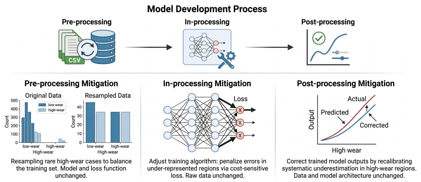
Figure 2.
Illustration of bias mitigation strategies throughout the machine learning model development lifecycle. The upper section shows the three stages at which mitigation can be applied: pre-processing, in-processing, and post-processing. In the pre-processing stage, class imbalance is addressed by resampling under-represented high-wear instances to create a more balanced training dataset. In the in-processing stage, the learning algorithm is modified through cost-sensitive training, where higher penalties are assigned to errors in minority or under-represented regions. In the post-processing stage, model predictions are recalibrated after training to correct systematic underestimation in high-wear regions. These approaches aim to improve predictive fairness and accuracy while operating at different stages of the machine learning pipeline
Figure 2.
Illustration of bias mitigation strategies throughout the machine learning model development lifecycle. The upper section shows the three stages at which mitigation can be applied: pre-processing, in-processing, and post-processing. In the pre-processing stage, class imbalance is addressed by resampling under-represented high-wear instances to create a more balanced training dataset. In the in-processing stage, the learning algorithm is modified through cost-sensitive training, where higher penalties are assigned to errors in minority or under-represented regions. In the post-processing stage, model predictions are recalibrated after training to correct systematic underestimation in high-wear regions. These approaches aim to improve predictive fairness and accuracy while operating at different stages of the machine learning pipeline
Each stage carries a different cost and a different benefit. Pre-processing is simple and model-agnostic but can introduce duplication or overfitting; in-processing is powerful but requires retraining and careful tuning; post-processing is fast and inexpensive to deploy but cannot recover information that the model never learned. A central question of this work is therefore not only whether bias can be reduced, but also which stage — or combination of stages — offers the largest reduction in high-wear error for the lowest cost.
1.4. Aim, Objectives, and Contributions
In response to the gap identified above, the aim of this work is to develop and evaluate a trustworthy AI framework for multimodal tool wear prediction that reduces the systematic underestimation (bias) of high-wear cases — the most safety-critical failure mode in CNC milling. The following objectives support this aim:
- 1.
- Build a single-modality baseline. Develop an image-only wear-regression model with no bias mitigation, reported with standard and per-bin error metrics, to serve as the reference point (Model 1).
- 2.
- Build a multimodal engineering baseline. Develop a fusion model that combines image features with sensor-derived features (force, acceleration, and acoustic signals), using established ML practice such as bin-weighted regression and class-weighted classification, and document the supporting design choices (Model 2).
- 3.
- Carry out a bias audit. Identify and quantify the main sources of bias in the pipeline — including wear-distribution skew, wear-type imbalance, and cross-material confounding — and summarise them in a quantified bias table.
- 4.
- Apply a lifecycle bias-mitigation pipeline. Reduce bias at the three stages defined in Section 1.3 — pre-processing (high-wear resampling: SMOTER, random over-sampling with Gaussian noise, and a combined over/under-sampling scheme), in-processing (cost-sensitive and relevance-based wear-bin weighting), and post-processing (conformal recalibration of the upper wear range) — selecting at each stage the method that genuinely reduces high-wear error without degrading the well-sampled region, and combining the selected methods into a mitigated model (Model 3).
- 5.
- Test model-independence and run a three-way comparison. Evaluate the image-only, multimodal, and mitigated models using both standard metrics (MAE, RMSE) and target-region fairness metrics (per-bin MAE gap, signed high-wear bias — where fairness denotes equitable model performance across the wear range, not demographic or social fairness), and then repeat the audit-and-mitigation pipeline across six regressor families (XGBoost, Random Forest, LightGBM, CatBoost, support-vector regression, and a multilayer perceptron) under an identical fused-feature representation, to establish whether any residual high-wear bias is specific to one model or common to all.
- 6.
- Test optimisation-independence and analyse the accuracy–fairness trade-off. Subject the model to a rigorous hyperparameter search (including and regularisation) and to bias-aware loss functions (quantile and asymmetric losses that explicitly penalise under-prediction), to determine whether the residual bias can be closed by dedicated optimisation; and characterise the accuracy–target-region fairness trade-off across mitigation intensity, identifying the configuration that offers the best high-wear target-region fairness for the lowest cost and translating the result into deployment guidance.
Contributions. This paper makes three contributions. First, it provides a reusable bias-evaluation protocol for safety-critical tool-wear regression that combines a signed, stratified bias audit with target-region fairness-disparity metrics (worn-region versus healthy-region MAE gap) and a three-stage mitigation lifecycle. Second, it presents an empirical demonstration, across six model families and under rigorous hyperparameter tuning and bias-aware losses, that lifecycle mitigation reduces but does not eliminate the high-wear bias: a residual, directional under-prediction persists in every configuration. Third, it contributes a diagnostic characterisation of this residual bias as data-intrinsic rather than model-reducible, demonstrated on a concrete, real-world case in which bias is present, measurable, and consequential. The MATWI dataset serves as the worked example: a CNC milling scenario in which the training data is structurally skewed toward low-wear conditions and the resulting model systematically under-estimates wear in exactly the region that matters most for safe operation. Together these contributions show manufacturers how the bias can be surfaced through signed, stratified auditing, how far lifecycle mitigation can reduce it, and — critically — that when it persists after mitigation the root cause is data adequacy rather than model design. The practical implication is direct: eliminating this class of bias begins not with a better algorithm but with a more representative data-collection strategy at the acquisition stage, targeting the high-wear operating conditions the model will be asked to predict. The work does not claim to eliminate the bias; its contribution is a principled means to evaluate it, to distinguish model-reducible from data-intrinsic bias, and to recognise when data collection — not further algorithmic correction — is the binding constraint. Table 1 situates the present work against representative prior studies, spanning the two fields it bridges: data-driven tool-wear prediction and bias-aware imbalanced regression. The comparison is read by capability rather than by performance. The dataset paper that introduces MATWI [12] provides multimodal data but evaluates only a vision-based model, without fusing the sensor channels; the attention-based study of [21] fuses multiple process sensors but uses no image modality; and the model-agnostic imbalanced-regression study of [15] addresses imbalance across several regressor families on general datasets, but not tool wear, and without a stratified bias audit or fairness-based evaluation. Across these works, predictive accuracy is the consistent objective, while the directional, safety-critical bias in the high-wear region, its mitigation across the modelling lifecycle, and the question of whether any residual bias is reducible at all are not examined. The present work occupies precisely that gap: it fuses the image and sensor modalities, audits the high-wear bias with signed and region-stratified metrics, applies a lifecycle mitigation pipeline, and tests the residual against both model family and optimisation to determine whether it is data-intrinsic. The marks in Table 1 denote the stated scope of each study and are not a judgement of its quality.
The work reported here completes the first stages of this programme. An exploratory analysis of the MATWI dataset confirms the conditions that make bias likely. The mean recorded wear is only about 110 m on a 0–450 m scale, so the data is heavily concentrated at low wear; roughly two-thirds of all measurements show pure flank wear, with adhesive and combined wear making up the remainder; and high-wear measurements are scarce, as most tools contribute mainly low-wear cuts. The dataset is therefore skewed in target value, imbalanced in wear type, and uneven in how well each wear region is represented.
Building on this analysis, two models have been developed and evaluated on 1,144 image–sensor measurements drawn from thirteen of the seventeen tools in the dataset. A single-modality image-regression model (Model 1, a fine-tuned ResNet-18) reaches a mean absolute error (MAE) of 51.4 m on the held-out test set. A multimodal fusion model (Model 2), which combines 512 image features with 84 sensor-derived features from the force, acceleration, and acoustic channels, lowers the test MAE to 30.9 m — a reduction of about 40% — and clearly outperforms a sensor-only model (68.3 m); its accompanying wear-type classifier separates normal flank wear from wear that needs inspection with a ROC-AUC of 0.93. Most importantly, a per-bin breakdown of these results confirms the central premise of the study: the error is not spread evenly. The baseline holds single-digit to low-double-digit MAE in the well-populated low-wear region, but under-predicts wear by roughly 85 m in the high-wear region — exactly the one-sided, safety-relevant bias that the mitigation stage is designed to reduce. A check for shortcut learning was also carried out, and it found that the learned image features track wear within each individual tool rather than only across tools, indicating that the model relies on genuine wear cues rather than on dataset confounders.
Headline findings. The central result of this work is that the high-wear under-prediction described above is reduced but not eliminated by mitigation applied across the full modelling lifecycle. Interventions at the data level (resampling of the raw high-wear cases), at the training level (cost-sensitive and relevance-based weighting), and at the output level (post-hoc recalibration) each lower the high-wear error but none close it, and the improvement is obtained only at some cost to the well-sampled low-wear region. The same bias persists across all six model families examined and survives both a rigorous hyperparameter search and bias-aware loss functions. The limitation is therefore shown to be data-intrinsic: the high-wear regime is too sparsely sampled for the relationship to be recovered by any redistribution of the existing data, so the effective remedy is the acquisition of more balanced, unbiased high-wear data rather than further refinement of the model. The supporting results are reported in full in Section 6.
Figure 3 gives a visual overview of the paper’s structure, mapping each section onto the trustworthy-AI context that motivates it and the six research objectives (O1–O6) it addresses.The remainder of this paper is organised as follows. Section 2 reviews related work on tool wear estimation and on trustworthy and bias-aware AI. Section 3 describes the MATWI dataset, and Section 4 presents the exploratory data analysis. Section 5 sets out the methodology, including the baseline models and the three-stage mitigation pipeline. Section 6 reports and discusses the results, and Section 7 concludes with the main findings and directions for future work.
2. Background
The Introduction established that trust is the principal barrier to deploying AI in safety-critical manufacturing, and that the one-sided underestimation of high-wear cases is the specific trust failure this work corrects. This section builds the foundation needed to diagnose it: how AI became embedded in manufacturing (Section 2.1) and how the technology has evolved (Section 2.2); what trustworthiness means and why bias is its most consequential failure (Section 2.3 and Section 2.4); and how regulators and standards bodies now respond (Section 2.5).
2.1. AI in Modern Manufacturing
Industry 4.0 connected machines, sensors, and processes into integrated cyber-physical systems, and AI and machine learning (ML) supplied the means to turn the resulting data into decisions. AI is now embedded across the production lifecycle — predictive maintenance, quality control, process optimisation, and supply-chain planning — shifting each from reactive correction toward anticipatory control [1,2]. This rests on an infrastructure layer that is easy to overlook: the Industrial Internet of Things (IIoT) instruments machines so that process signals — vibration, cutting force, acoustic emission, and images of the cutting edge — are captured continuously [22], while lightweight protocols such as MQTT, 5G networks, and edge computing move this telemetry off the shop floor and run inference close to the machine [22]. Together these form a stack from shop-floor sensing to model-driven decision (Figure 4). How data is captured and managed at this layer determines whether a model is later trained on a representative record of the process or a partial one — the distinction that, as Section 2.4 shows, lies at the root of the bias addressed here.
The role of the human has been re-examined in parallel. Where Industry 4.0 emphasised automation, the emerging Industry 5.0 paradigm re-centres the operator, framing AI as augmenting rather than replacing human capability [7,8]: the model produces a recommendation that a human interprets, validates, or overrides before action. This collaboration is not automatic — a persistent automation–augmentation tension must be actively managed [9] — and it requires operators to be upskilled to judge model outputs and intervene appropriately [7,9]. Running through the instrumentation, connectivity, and human-in-the-loop design is a single objective: consistent, verifiable product quality [1,2]. This is why model reliability cannot be treated as a convenience: an erroneous decision in this setting carries real safety and financial cost.
2.2. The State of the Art in AI for Manufacturing
The AI deployed in manufacturing is a layered progression of paradigms; tracing it shows why the field has moved toward richer, multi-source models and locates the multimodal approach used here within the current state of the art. The foundation remains discriminative deep learning — convolutional networks for visual inspection and recurrent or convolutional networks for sensor-signal regression, the workhorses of defect detection, fault diagnosis, and wear estimation [22]. Their limitation is directly relevant: they are only as good as their labelled data, and the most safety-critical states — severe defects, advanced wear, imminent failure — occur least often. This scarcity is the recurring constraint that the subsequent paradigms each attempt to relax.
The first response was generative AI: generative adversarial networks (GANs) and, more recently, diffusion models synthesise realistic samples, most commonly to augment rare defect classes and rebalance skewed training sets [23]. This frames synthetic rebalancing as one established lever for data imbalance — a lever this paper revisits, in its pre-processing stage, for continuous-valued regression rather than discrete classes. A more recent shift is the arrival of large language models (LLMs) and multimodal LLMs (MLLMs), which integrate visual, sensor, and structured data within a single model for more context-aware interpretation of a process [24]. The principle behind them — that complementary data sources yield a more complete and reliable picture than any single source — also underpins multi-sensor fusion for machinery prognostics, where imagery, vibration, cutting force, and acoustic emission are combined to estimate tool condition more robustly than any modality alone [21]. This is the paradigm to which the present work belongs. The current frontier is agentic AI — systems that plan and act toward a goal with limited human intervention, increasingly as cooperating multi-agent systems [24]; for a trustworthiness study this frontier is a warning, since the more autonomy a model is granted, the more consequential an undetected systematic error becomes, as less human judgement is positioned to catch it.
Two threads run through this progression and motivate the rest of the Background. First, every paradigm is constrained by the quantity and balance of its training data, and the high-wear scarcity identified in the Introduction is a structural feature of the setting, not an artefact of one model choice. Second, as models grow more capable and autonomous, human oversight does not scale at the same rate. Both point to the same requirement: a principled account of what makes an AI system trustworthy, and of why bias is the trust failure that matters most.
2.3. Trustworthy AI: Principles and Why They Matter
Trustworthy AI (TAI) is best understood not as a single property but as a set of characteristics an AI system must jointly satisfy, and there is now substantial convergence on what these are. The NIST AI Risk Management Framework lists systems that are valid and reliable, safe, secure and resilient, accountable and transparent, explainable, privacy-enhanced, and fair with harmful bias managed [25]; the OECD AI Principles [26] and a synthesis of the academic literature by Li et al. [27] articulate closely aligned sets. Five pillars recur that bear directly on this work (Figure 5). Reliability and robustness concern whether a model performs validly and consistently under the variation, noise, and distribution shift of normal operation [25,26]. Transparency and explainability concern whether the basis of an output can be scrutinised [25,27] — without which an operator cannot distinguish a well-grounded estimate from a shortcut or an extrapolation into a data-sparse region. Accountability concerns whether responsibility for a system’s behaviour can be traced and assigned [26,27], and safety and security whether the system avoids harm under foreseeable or adverse conditions and resists manipulation [25,26] — in CNC machining, an unsafe wear-prediction error translates directly into tool failure and physical risk.
Fairness, the fifth pillar, is the direct concern of this work and requires precise definition. In mainstream AI ethics fairness is usually social fairness: equitable treatment across demographic groups defined by protected attributes such as gender, race, or age. This paper does not address social, anti-discrimination, or protected-attribute fairness; no demographic or personal data is involved in the MATWI dataset or the models built from it [20]. The concern here is target-region fairness: that a regression model performs equitably across the range of its prediction target rather than concentrating its errors in a specific, safety-critical sub-region. The disadvantaged “group” is not a demographic class but the high-wear regime (m) of a continuous wear target; the principle is structurally identical — a model ought not to perform systematically worse for one identifiable sub-population of its input space — but the sub-population is defined by the target value, not by any human attribute.
These pillars are interdependent: a model may be robust yet opaque, or accurate on average yet unfair, and a deficiency in any single one is sufficient to make the system as a whole untrustworthy — high average accuracy does not compensate for a failure of fairness. Trustworthiness is also the precondition for the human–AI collaboration of Section 2.1: an operator can only accept, question, or override a recommendation if the model is reliable, its reasoning legible, and its errors not systematically concentrated where they are most dangerous. The trust failure identified in the Introduction — the systematic underestimation of high-wear cases — is, in formal terms, a fairness failure, and is the subject of the next section.
2.4. Bias as a Trustworthiness Failure
This work uses bias in its technical sense: a systematic, non-random error in which a model’s predictions are skewed against an identifiable region of the input or output space. The mechanism is the same as in social bias — a model performs unevenly across a space it ought to treat uniformly, and the analytical tools transfer directly [20] — but here the disadvantaged region is the high-wear regime of a continuous target rather than a demographic group. A central insight of the fairness literature is that bias enters not at a single point but at multiple, distinct stages of the ML lifecycle. Suresh and Guttag [28] give the widely adopted account; four of their sources are directly relevant (Figure 6). Historical bias arises when accurately collected data reflects a state of the world the model should not reproduce. Representation bias arises when the training data under-samples part of the population the model will face — the dominant source here, since high-wear cuts are, by operational design, rare relative to healthy ones. Measurement bias arises when features or labels are imperfect proxies for the quantity of interest — a risk wherever wear is inferred indirectly, or confounders such as material or wear type co-vary with the label. Aggregation bias arises when one model is applied uniformly to sub-groups that behave differently, learning an average pattern that fits none well — a tangible concern in a multi-material, multi-wear-type dataset.
A fifth source, evaluation bias, explains why bias so often goes unnoticed: it arises when a model is judged by metrics that do not reflect its intended use [28]. The most common form is a single aggregate score — an overall RMSE or R2 averages across the whole target range and can conceal severe underperformance in a small but critical sub-region. This directly motivates the disaggregated, per-bin and fairness-oriented evaluation adopted in this study. The consequence is acute in manufacturing: a model that underestimates high wear reports a worn tool as healthier than it is and so defers replacement past the safe point, risking degraded quality, scrap, and — in the limit — tool failure and unplanned downtime. The bias is directional, its burden falling entirely on the most consequential failure mode; and, as Section 2.2 noted, growing autonomy makes a bias not surfaced by evaluation increasingly unlikely to be caught by an operator. Two conclusions frame the methodology: because bias enters at several lifecycle stages, mitigation must itself be staged (the pre-, in-, and post-processing pipeline of the Introduction); and bias must be made visible, through disaggregated evaluation, before it can be managed.
2.5. Governance, Standards, and the Regulatory Landscape
Trustworthiness, and bias mitigation in particular, is no longer a purely technical requirement: over the past few years it has become the subject of an active, fast-moving body of governmental policy, regulation, and international standardisation. The global picture reads as a spectrum from prescriptive, legally binding regulation to light-touch, principles-based guidance — yet, as Table 2 shows, this divergence in legal form conceals a striking agreement on substance: every major framework identifies the avoidance of unfair bias as a defining element of trustworthy AI. The European Union occupies the prescriptive end. The EU AI Act (Regulation (EU) 2024/1689), in force since August 2024, is the first comprehensive horizontal AI law and scales obligations with the potential for harm [29]; its obligations for high-risk systems — a category that includes AI used as a safety component in critical infrastructure and machinery — are scheduled to apply from August 2028 [29]. Tool-condition monitoring in a safety-relevant production context falls within the spirit of this high-risk tier, and the Act’s requirements for data quality, accuracy, and risk management speak directly to the bias concern of this paper.
The United Kingdom, where this work is carried out, has taken a deliberately different, principles-based and sector-led route. The National AI Strategy (2021) set a ten-year framework whose governance pillar became the 2023 White Paper, A Pro-Innovation Approach to AI Regulation, defining five cross-sector principles — safety, security and robustness; transparency and explainability; fairness; accountability and governance; and contestability and redress — to be applied by existing regulators [30,31]. This is reinforced by the AI Safety Institute (since reframed as the AI Security Institute), which conducts model evaluation, and by the Advanced Research and Invention Agency’s Safeguarded AI programme, which funds work toward quantitative safety guarantees for safety-critical domains including manufacturing [32]. The framework’s fairness principle and its emphasis on verifiable reliability align closely with this study.
The remaining major jurisdictions span the spectrum. The United States has taken a market-driven, innovation-first federal posture in which the voluntary NIST AI RMF functions as the de facto reference for trustworthy-AI practice and explicitly names fairness with harmful bias managed [25]. China regulates particular applications vertically — most prominently generative-AI services and the labelling of AI-generated content — rather than through a single horizontal law. India has issued the light-touch India AI Governance Guidelines (2025) under the IndiaAI Mission, anchored in principles that include fairness, transparency, accountability, and safety [33], building on NITI Aayog’s earlier Responsible AI for All (2021) [34]. Cutting across these national approaches is a layer of international standardisation: ISO/IEC TR 24028:2020 established a shared vocabulary framing fairness as the avoidance of unjust discrimination [35], and ISO/IEC 42001:2023 provides the first auditable AI-management-system standard, with explicit attention to transparency, fairness, and lifecycle risk [36]; the IEEE’s Ethically Aligned Design adds engineering-oriented guidance to the same end [37].
The observation to draw from this survey is one of convergence. The jurisdictions differ markedly in legal form — binding regulation in the EU, principles and sector regulators in the UK, voluntary frameworks in the US, vertical measures in China, light-touch guidance in India — yet they do not differ on substance: every framework identifies fairness, and the active management of harmful bias, as a core requirement of trustworthy AI. The systematic underestimation of high-wear cases addressed by this paper is therefore not only a technical shortcoming and a safety hazard, as Section 2.3 and Section 2.4 established, but also a failure to meet an expectation now common to AI governance worldwide. Having established why this bias must be identified and mitigated, the work now turns to how it is achieved for multimodal tool-wear prediction on the MATWI dataset.
3. The MATWI Dataset
This study uses the Multimodal Automatic Tool Wear Inspection (MATWI) dataset, introduced by De Pauw et al. [12] and made publicly available via the KU Leuven EAVISE repository [38]. MATWI was created to address a specific obstacle in data-driven tool-wear research: deep-learning methods require large datasets, yet wear datasets recorded on real production machinery are scarce. MATWI was assembled to fill that gap, and it is, to the authors’ knowledge, the first dataset to pair image data with accelerometer, microphone, and force measurements captured continuously along the life of a cutting tool [12].
The dataset records the wear of carbide milling inserts during real computer numerical control (CNC) milling. Seventeen separate cutting tools were each run from a new condition until end of life, and approximately one hundred measurements were taken across the lifespan of each tool [12], yielding 1,663 expert-labelled measurements in total [12]. Each measurement corresponds to a single milling pass, hereafter referred to as a cut: for every cut, an image of the cutting edge is captured and the process is monitored by a set of sensors. The quantity of interest is flank wear, the gradual recession of the cutting edge that develops during milling and is the standard indicator of an insert’s condition [12]. The paper introducing MATWI reports that the wear values it contains span approximately 45 to 450 m, together with a single outlier of about 750 m attributable to adhesive build-up on the insert [12]; the upper end of this range corresponds to roughly the width of four human hairs. Judging wear at this scale reliably by eye is difficult, which is precisely why an automated, sensor-supported estimate is valuable [12].
The data was acquired with a purpose-built measurement setup designed to be installable on a real production-level CNC machine, so that the same acquisition procedure could, in principle, be deployed in operational use [12]. The setup has two parts: the CNC machine itself, which reports the position of its spindle, and a separate camera box containing a macro lens, a controller, and lighting. For every cut, the milling program executes a single pass through the workpiece; sensor measurements are recorded from before the tool enters the workpiece until after it exits, and an image of the insert’s cutting edge is captured at the end of the pass, while the machine is stationary [12]. Because the CNC controller and the camera-box controller cannot communicate bidirectionally, the two are synchronised indirectly: the camera-box controller monitors the spindle position reported by the machine and triggers image capture, or begins and ends sensor recording, when the spindle reaches a predefined location [12]. This indirect synchronisation is important to record here, because — as Section 3.2 and Section 4 will show — it is the origin of several of the data-completeness gaps that the curation process must later handle. The sensing hardware itself is documented in detail by the dataset authors: process vibration is measured by a PCB Piezotronics 333B40 accelerometer, acoustic emission by a Vallen CS30 sensor, and cutting force along three axes by a Kistler 9255C force-measurement table, all sampled synchronously [12]. Figure 7 summarises the acquisition arrangement.

Table 3.
The three data modalities provided by the MATWI dataset. The image is a direct observation of the tool’s condition; the sensor signals are an indirect observation of the process; the process parameters are fixed configuration.
Table 3.
The three data modalities provided by the MATWI dataset. The image is a direct observation of the tool’s condition; the sensor signals are an indirect observation of the process; the process parameters are fixed configuration.
| Modality | Content | Granularity | Relation to wear |
|---|---|---|---|
| Image | One cutting-edge photograph, RGB JPEG | Per cut | Direct observation |
| Sensor | Five signal channels (accelerometer, acoustic emission, force x/y/z) plus timestamp; no header; variable length; 1626 Hz | Per cut | Indirect observation |
| Process parameters | Cutting speed, rotation speed, feed, depth of cut, material, supplied crop region | Per tool (set) | Fixed configuration |
In summary, MATWI provides a large, real-world, and genuinely multimodal record of carbide-insert wear: seventeen tools followed to failure, around one hundred cuts each, with every cut pairing a microscope image of the cutting edge against synchronised force, vibration, and acoustic signals. These properties make it well suited to the trustworthy-wear-prediction study undertaken here. The following section specifies exactly how this information is structured and stored, which is necessary background for the data-curation and modelling decisions that follow.
3.1. Data Structure and Modalities
Having described how MATWI was acquired, this section specifies how the data is organised, since the modelling pipeline of this paper operates directly on that structure. The dataset is organised around the cut as its fundamental unit. Each cut corresponds to one milling pass and is described by a single row in a central index file, labels.csv, which the present study found to contain 1,803 rows across 11 columns. Each row records the identifiers of the cut — the tool (or set) it belongs to and its position in that tool’s life — together with the measured flank-wear value, a wear-type label, and the file paths to that cut’s image and sensor recording. A second file, sets.csv, holds information that is constant within a tool but varies between tools, namely the cutting parameters and workpiece properties. The two files therefore separate per-cut measurements from per-tool configuration, and are joined on the set identifier. Table 3 summarises the three data modalities the dataset provides; each is described below.
The image modality provides, for every cut, one photograph of the insert’s cutting edge captured by the macro-lens camera. These are high-resolution RGB images: inspection in this study confirmed a consistent resolution of pixels across the dataset, stored in JPEG format, consistent with the 20-megapixel camera reported by the dataset authors [12]. A representative image is shown in Figure 8. The visual content of interest — the worn region of the cutting edge — occupies only a fraction of the frame, while the remainder contains background and, on some tools, engraved workpiece identifiers. The dataset authors anticipated this and additionally supply, for each set, a rectangular crop region isolating the cutting edge [12]; the use of the full image versus this supplied crop is a preprocessing decision addressed in the Methodology. The image is a direct measurement of wear: it depicts the physical condition of the tool itself.
The sensor modality provides, for every cut, one multi-channel time-series recording of the milling process. Each recording is stored as a comma-separated file with no header row, comprising five signal channels together with a timestamp column. The five signal channels are the accelerometer, the acoustic-emission sensor, and the three force axes (force in x, y, and z) described in Section 3. The recordings are of variable length, since the duration of a milling pass is not fixed; the dataset authors report that the five sensors are sampled synchronously at 1626 Hz [12], and a representative cut examined in this study contained on the order of samples per channel. Unlike the image, these signals are an indirect measurement of wear: they record the process behaviour — vibration, sound, and cutting force — from which the tool’s condition must be inferred. Figure 9 shows the five signal channels of one representative cut. Two structural properties of this modality are important for the analysis that follows and are returned to in Section 4: the recordings vary in length from cut to cut, and the number of active channels is not constant across cuts.
The process-parameter modality, held in sets.csv, provides the controlled settings under which each tool was run. The dataset authors record, for each set, the cutting speed, the rotation speed, the feed per tooth, the feed rate, the cutting width and the cutting depth, together with the workpiece material and the supplied image crop region [12]. Unlike the image and sensor data, these values are not measurements taken during a cut but fixed configuration parameters; they vary between tools but are constant for all cuts of a given tool. They provide context for interpreting the measured signals rather than a direct or indirect observation of wear. It should be noted that the cutting parameters for the first set were not recorded by the dataset authors [12], a gap returned to in Section 4.
In combination, these three modalities give, for every cut, a direct visual record of the tool, an indirect dynamic record of the process, and the configuration under which both were produced. This structure is what makes MATWI suitable for multimodal modelling. It also, however, introduces the practical complications — variable-length recordings, non-uniform channel availability, and incomplete records — that any model must accommodate. The next section characterises the seventeen tools the dataset contains and documents these data-quality issues explicitly.
3.2. Cohort Characteristics and Known Anomalies
The seventeen tools in MATWI do not form a uniform cohort; they differ in workpiece material, in cutting parameters, and in the range of wear they reach. Characterising this variation is necessary because it determines both how the data must be partitioned for modelling and which tools can be used at all. This section describes the cohort and then documents, explicitly, the data-quality anomalies that the curation process in Section 4 must address.
The clearest division within the cohort is the workpiece material. Tools 1 to 11 were run on CK45 carbon steel, while tools 12 to 17 were run on RVS 304 stainless steel [12]. This distinction is not incidental: the dataset authors note that the change of material can produce different wear types on the inserts, and stainless steel in particular is associated with more adhesive wear. The cutting parameters also vary between tools — the early CK45 tools span a wide range of cutting and rotation speeds, while the later tools were run at the settings reported for the RVS 304 material [12]. Each tool therefore represents a slightly different machining condition, which is why, as Section 4 explains, the dataset must be partitioned at the level of whole tools rather than individual cuts.
Table 4 summarises the per-set wear characteristics measured in this study. Several features of the cohort are visible in it. The number of cuts per tool varies from 50 to roughly 150. More importantly, the wear range covered differs sharply between tools: most tools remain well below the 450 m measurement ceiling, reaching maxima between 90 and 300 m, and only Set 5 traverses the full wear range up to 450 m. The mean wear of most tools sits in the low hundreds of micrometres or below, confirming that the high-wear regime is sparsely sampled across the cohort as a whole — an observation developed quantitatively in Section 4.
Alongside this natural variation, the dataset contains a number of specific data-quality anomalies that were identified during the curation carried out for this study. Documenting them here is essential, both for transparency and because they directly explain the curation decisions described in Section 4.
The first anomaly concerns an extreme wear value. As reported by the dataset authors and confirmed in Table 4, Set 11 contains a single cut with a measured wear of 750 m, well beyond the 450 m ceiling that characterises the rest of the dataset [12]. This is consistent with adhesive build-up, in which workpiece material adheres to the insert and produces an apparent wear value larger than the insert itself. It is treated as an outlier in the analysis that follows.
The second and third anomalies concern the sensor channels. A per-cut inspection of channel activity carried out in this study found that, of the five signal channels, four (the accelerometer, the acoustic-emission sensor, and two of the three force axes) are active in every cut, but the remaining force channel is inactive in 10.1% of cuts in the modelling corpus: of the 1,144 cuts, 1,029 carry all five channels (89.9%) and 115 carry only four (10.1%). This inactive-channel behaviour is concentrated in particular tools rather than spread uniformly; Set 5, for example, lacks that channel across all of its cuts. A more severe instance of the same problem affects Set 3, in which every cut was found to retain only two of the five sensor channels. Because the modelling approach in this paper depends on combining image and sensor information, a tool whose sensor recording is reduced to two channels cannot contribute usable multimodal examples; Set 3 is therefore excluded from the study for this reason.
A fourth issue concerns the process parameters rather than the measurements: as noted in Section 3.1, the cutting parameters for Set 1 were not recorded by the dataset authors [12], so this tool carries complete image and sensor data but incomplete configuration metadata.
Taken together with Set 2 and Set 17, which exhibited the same sensor-channel degradation as Set 3 and were excluded on the same grounds, and with Set 14, a pilot run used during initial dataset assembly whose cutting-parameter configuration was not finalised at the time of recording and which was therefore excluded from the modelling corpus, these anomalies mean that the seventeen-tool dataset cannot be used in its entirety.
4. Exploratory Data Analysis
Section 3 described the MATWI dataset as it is supplied. This section analyses it. The analysis has two purposes: to establish how the data must be curated and partitioned before any model can be trained on it, and to build, step by step, the evidence for the central modelling decision of this paper — that tool wear cannot be predicted reliably from any single source of information, and that a multimodal approach is therefore required. The section proceeds as a continuous argument: it begins with curation, then characterises the wear target and its imbalance, then examines in turn each candidate source of predictive information — process parameters, sensor signals, and images — before drawing these threads together. Each step is supported by a figure produced during the analysis.
Data curation and the experimental split:The anomalies documented in Section 3.2 mean that the seventeen-tool dataset cannot be passed to a model unfiltered. Two curation steps are therefore applied. The first is a usability filter at the level of the individual cut: a cut is retained only if it has a valid image, a valid sensor recording, and a recorded wear value, since a cut missing any of these cannot serve as a complete multimodal training example. Applying this filter to the raw index reduces the dataset to 1,566 usable cuts across all seventeen tools, including the four that are subsequently excluded at the tool level. The proportion of cuts removed is not uniform across tools — it ranges from a few per cent for the cleanest tools to roughly a quarter for the most affected — a direct consequence of the synchronisation and channel issues described earlier.
The second curation step divides the retained cuts into training, validation, and test partitions. As established in Section 3.2, the tools differ in material and cutting conditions, and the cuts within a tool are highly similar to one another; partitioning at the level of individual cuts would therefore allow near-identical cuts from the same tool to appear in both training and test data, producing an optimistic and misleading estimate of performance. To prevent this, the dataset is partitioned at the level of whole tools: every cut from a given tool is assigned entirely to one partition. The resulting split is summarised in Figure 10. The training partition comprises tools 1, 5, 7, 8, 10, and 12 (501 cuts); the validation partition tools 6, 13, and 15 (247 cuts); and the test partition tools 4, 9, 11, and 16 (396 cuts). The four excluded tools — Sets 2, 3, 14, and 17 — are set aside for the reasons given in Section 3.2: Sets 2, 3, and 17 for sensor-channel degradation, and Set 14 as a pilot run excluded from the modelling corpus. Of the 1,566 cuts that pass the per-cut filter, 422 belong to these four excluded tools; the modelling corpus therefore comprises cuts, divided as stated in Table 5.
Two properties of this split are important for all later results. First, the spread of wear differs between partitions: the training partition spans the widest range, from 15 m to the full 450 m ceiling, while validation and test reach 210 m and 750 m respectively, with median wear of 60 m in training and 90 m in validation and test. Even in the training partition, the high-wear region is thinly populated: only about one in six training cuts lies in the most safety-critical region of the wear scale. Second, the training partition is predominantly CK45 steel with a single RVS 304 tool, whereas validation and test each mix the two materials — so the model sees both materials, but unevenly.
What curation removed, and why: Before characterising the data that was kept, it is worth examining what was lost. Figure 11 shows, for every tool, two complementary views of data quality. Panels (a)–(c) count missing rows — cuts for which an image, a sensor recording, or a wear-type label was never written — and show this incompleteness is concentrated in particular tools rather than spread uniformly. This is the direct fingerprint of the indirect controller synchronisation described in Section 3: when the camera-box controller and the CNC machine fall out of step, a recording for that cut is simply never written, which is why the usability filter removes a very different fraction of cuts from one tool than from another.
Panel (d) shows a different and more operationally consequential form of incompleteness: the fraction of cuts per tool in which all three force channels are active. This panel makes the tool-level exclusion criterion visible. Sets 2, 3, and 17 show near-zero or very low force-channel activity across their entire tool run — not isolated missing cuts, but a pervasive hardware condition that renders the sensor modality unusable for the whole tool. These three sets are therefore excluded at the tool level, as documented in Section 3.2. Set 14 is also excluded, but for a different reason (non-finalised cutting parameters in a pilot run, also documented in Section 2.8), and its channel activity in panel (d) is accordingly unaffected. Set 6 appears elevated in panel (a) due to missing wear-type labels, but panel (d) shows its force-channel anomaly is localised to individual cuts rather than the full tool run; it is retained in the modelling corpus, with only the affected cuts removed by the per-cut filter. The distinction between tool-level exclusion (Sets 2, 3, 14, and 17) and cut-level removal (Set 6 and others) is the operative curation criterion that produces the 1,144-cut modelling corpus from the 1,566 cuts that pass the per-cut filter.
The wear target is severely skewed: With the usable data established, the analysis turns to the quantity the model must predict: flank wear. Figure 12 shows the distribution of wear values. The distribution is heavily skewed toward low wear: the large majority of cuts record a healthy or lightly worn tool, and high-wear cuts are comparatively rare. This is not a defect of the dataset but an inherent property of the process — a tool spends most of its life in good condition and only briefly approaches end of life — yet it has a direct and serious modelling consequence. A regression model trained on such a distribution under a conventional error criterion is dominated by the densely populated low-wear region, and it can minimise its average error by predicting toward the centre of the distribution, systematically under-predicting the rare high-wear cuts. The skew visible in this figure is thus the root cause of the high-wear underestimation that this paper sets out to address.
Wear coverage is uneven across tools: The skew is compounded by a second effect: the tools do not each cover the wear range equally. Figure 13 summarises, per tool, the wear range traversed and its mean, maximum, and variability. Most tools remain confined to the lower part of the wear scale, never approaching the measurement ceiling; only one tool, Set 5, traverses the full range to 450 m, and one further tool, Set 11, contains the single 750 m outlier discussed in Section 3.2. The high-wear examples that do exist are therefore not only few in number but concentrated in a small number of tools. Because the data is partitioned by whole tools, this means the model’s exposure to high wear during training depends heavily on a handful of tools — a fragility that the per-tool evaluation in the Results section examines directly.
Wear types are imbalanced: Wear is not a single phenomenon. MATWI labels each cut by wear type — predominantly flank wear, with smaller numbers of adhesive and combined wear. Figure 14 shows the composition of wear types, both overall and across the partitions. Flank wear is by far the most common type, and the minority types are distributed unevenly between tools and therefore between partitions. This is a second axis of imbalance, distinct from the wear-value skew: even where a model sees enough examples at a given wear level, those examples may be dominated by one wear type, so its behaviour on the rarer types is supported by far less data. Wear-type imbalance is therefore a further source of uneven model reliability, and it is one reason the analysis below also considers a wear-type classification task alongside wear regression.
Cutting parameters alone do not determine wear: Having characterised the target and its imbalance, the analysis now examines the candidate sources of predictive information, beginning with the simplest. Each tool was run with known cutting parameters — cutting speed, feed, and depth of cut — and a natural question is whether these settings alone predict wear. Figure 15 plots wear against each parameter. They do not: at any given setting, the observed wear spans a wide range, because wear depends not only on the controlled parameters but on the elapsed cutting time, the workpiece material, and tool-to-tool variation. The cutting parameters provide context but are far from sufficient as predictors on their own. This is the first concrete piece of the multimodal argument: a model restricted to the process configuration cannot estimate wear, so a richer source of information — one that observes the tool or the process directly — is required.
The sensor signals carry information about wear: The first richer source is the sensor modality. Figure 16 summarises the behaviour of the five sensor channels across the tools, showing how the statistical character of each channel varies from tool to tool. The channels are not inert: their distributions shift in ways that track the machining condition, indicating that the vibration, acoustic, and force signals carry information relevant to wear. The figure also makes visible the channel-availability issue documented in Section 3.2 — one force channel is inactive in a substantial minority of cuts — so while the sensor modality is informative, it is also incomplete, and any model using it must tolerate missing channels.
Sensor-derived features correlate with wear — but partially: To assess the sensor signals more directly, summary features were extracted from each recording and examined against wear. Figure 17 reports this analysis: it shows which extracted features carry a usable signal, how their distributions behave, and the strength of their association with the wear value. Several features show a clear, non-trivial correlation with wear, confirming the sensor modality as a genuine predictor rather than noise. The associations are, however, only moderate in strength and are accompanied by the missing-channel effect noted above. The sensor signals are thus informative but not, on their own, a complete basis for accurate wear estimation — the second piece of the multimodal argument.
The images carry a genuine wear signal: The second richer source is the image modality. Figure 18 examines the visual content of the cutting-edge images: it presents representative images alongside a comparison of the average appearance of low-wear and high-wear cuts. The comparison shows a clear and physically interpretable difference — the worn region of the cutting edge changes in a consistent way as wear increases — confirming that the images contain a direct visual signature of wear. Because the images also contain background and, on some tools, engraved identifiers, it is important to establish that a model would key on the wear itself rather than on these incidental cues; this concern is taken up explicitly in the Methodology and Results, where the image model is audited for exactly this kind of shortcut. For the present purpose, the figure establishes the image modality as a strong, direct source of wear information.
Why a multimodal approach is required: The analysis can now be drawn together. The exploratory findings form a single argument. The wear target is severely skewed and unevenly covered, so the high-wear regime is intrinsically data-poor. The cutting parameters alone do not determine wear. The sensor signals carry genuine but only moderate predictive information, and are affected by missing channels. The images carry a strong and direct visual signature of wear, but capture only the surface appearance of the tool, not the dynamic behaviour of the cutting process. No single source is sufficient on its own: each is partial, and — critically — each is partial in a different way. The image observes the tool directly; the sensors observe the process the tool is part of. These are complementary views, and combining them offers information that neither provides alone. This is the evidence base for the central decision of this paper: to predict tool wear with a multimodal model that fuses the image and sensor modalities. The design of that model, and the way it is trained and evaluated, are the subject of the next section.
5. Methodology
This section sets out the methodology of the study. It is organised to mirror the research objectives stated in the Introduction: it first presents the overall framework that links those objectives into a single experimental programme (Section 5.1), then describes the data preparation common to every stage (Section 5.2), the two predictive baselines that have been constructed — an image-only model and a multimodal model (Section 5.3 and Section 5.4) — and finally the bias audit and the three-stage mitigation, comparison, and trade-off analysis that the framework is designed to support (Section 5.5, Section 5.6, Section 5.7 and Section 5.8).
5.1. Overall Framework
The central problem this work addresses is not merely to predict tool wear accurately, but to do so trustworthily — in particular, to identify and reduce the systematic underestimation of high-wear cases established in the exploratory analysis. Achieving this requires more than a single model; it requires a sequence of stages in which a predictor is first built, its bias is then measured, and that bias is subsequently mitigated and re-evaluated. The overall framework, shown in Figure 19, organises the six objectives of the study into exactly this sequence.
The programme proceeds as follows. A predictive model is first established in two steps: an image-only baseline (Objective 1), which uses the directly observed condition of the tool, and a multimodal baseline (Objective 2), which fuses the image with the process sensor signals to improve accuracy. These two models have been constructed and are described in detail below. The multimodal baseline then serves as the subject of a formal bias audit (Objective 3), which quantifies where and by how much the model’s errors are systematically concentrated. Informed by that audit, a three-stage mitigation strategy (Objective 4) is applied across the machine-learning lifecycle — before training (pre-processing), during training (in-processing), and after training (post-processing) — to produce a bias-mitigated model. The baselines and the mitigated model are then compared (Objective 5), and the relationship between overall accuracy and high-wear fairness is examined to characterise the trade-off involved (Objective 6). The audit, mitigation, comparison, and trade-off stages constitute the designed methodology that the constructed baselines are built to support.
5.2. Data Preparation and Experimental Split
All models operate on the curated MATWI dataset and the tool-level partition described in Section 4. Two points of the preparation are common to every stage and are restated here because they bear directly on the bias question. First, the dataset is partitioned by whole tools, so that all cuts from a given tool fall entirely within one of the training, validation, or test partitions; this prevents the near-identical cuts of a single tool from leaking between training and evaluation and inflating apparent performance. Second, the regression target is the measured flank wear, clipped at the upper end of the valid measurement range so that the single extreme outlier identified in Section 3.2 does not distort training. These choices fix a consistent basis on which every model in the programme is trained and judged.
5.3. Image-Only Baseline (Objective 1)
The first model predicts wear from the cutting-edge image alone, and establishes how much of the wear signal is recoverable from the directly observed condition of the tool. It is a convolutional neural network built on a ResNet-18 backbone, with its final classification layer replaced by a dropout layer and a single linear unit for scalar regression. The network is partially fine-tuned: the early convolutional stages, which capture generic low-level image structure, are frozen, while the deeper residual blocks and the regression head are trained on the wear task. Partial fine-tuning is appropriate for a training set of a few hundred images, adapting the high-level representation to the wear domain without the data demand of training all parameters afresh.
Each image is resized and, during training only, augmented by a random resized crop, a horizontal flip, a small rotation, and mild colour jitter, before normalisation. The spatial augmentation is deliberate: as the exploratory analysis noted, the images contain background and, on some tools, engraved workpiece identifiers, and randomising the position and appearance of such incidental marks between training views discourages the network from associating them with wear rather than learning the wear itself. Isolating the cutting edge by region-of-interest cropping was investigated but not adopted; the final pipeline operates on the full frame with augmentation. No augmentation is applied at validation or test time, so evaluation is deterministic. The network is trained with a Huber regression loss, which is robust to the residual outliers in the target, using the AdamW optimiser with a cosine-annealing schedule and early stopping on the validation error. The complete procedure is given in Algorithm 1, and the architecture is shown in Figure 20.
| Algorithm 1 Image-Only Wear-Regression Baseline (Objective 1) |
|
| Algorithm 2 Multimodal Feature-Level Fusion: Training and Inference (Objective 2) |
|
5.4. Multimodal Model (Objective 2)
The second model improves on the image-only baseline by adding the process sensor signals, on the rationale — established in the exploratory analysis — that the image and the sensors provide complementary, individually incomplete views of the same process. It uses an intermediate, feature-level fusion design: each modality is independently encoded into a fixed-length feature vector, the two vectors are concatenated, and a single learner is trained on the combined representation. The complete pipeline is shown in Figure 21.
This fusion strategy is dictated by the data rather than chosen by preference. Early (raw-input) fusion is infeasible: the image is a fixed pixel grid whereas the sensor recording is a variable-length, multi-channel time series of the order of samples, so the two cannot be expressed in a common raw tensor; the sensor recordings are moreover of variable length and inconsistent channel availability across cuts. Encoding each modality into a fixed-width descriptor is therefore a precondition for combining them at all, which makes feature-level fusion the necessary approach. Late (decision-level) fusion, in which each modality yields an independent prediction that are then averaged, was not adopted because it forgoes the cross-modal interactions a single learner over the joint feature space can capture.
Image branch: The image branch is the fine-tuned ResNet-18 of Section 5.3, reused as a feature extractor. After training, the activation of the network’s global average-pooling layer is taken, for each cut, as a 512-dimensional image feature vector summarising the visual evidence of wear.
Sensor branch: The sensor branch converts each variable-length, multi-channel recording into a fixed-length vector of hand-crafted features. Hand-crafted descriptors, rather than a learned sequence model, are appropriate for the small number of training cuts, for which a high-capacity temporal network would over-fit; the chosen features are the standard signal-processing summaries of the predictive-maintenance literature. The channels are handled according to role. One channel was verified, across every tool, to carry the acoustic-emission signal and is described with audio-style features, including mel-frequency cepstral coefficients and spectral summaries. The remaining accelerometer and force channels are each summarised with a common set of generic descriptors: time-domain statistics (root-mean-square energy, mean, standard deviation, skewness, kurtosis, peak-to-peak range, crest factor, and threshold-exceeding peak counts) and frequency-domain summaries from the power spectrum (the dominant frequency in the spindle band and its amplitude, the spectral entropy, and the spectral centroid), the latter computed on a decimated copy of the signal to reduce computation without affecting the spindle band. Where a channel is inactive in a given cut — a condition that, as the exploratory analysis showed, affects one force channel in a substantial minority of cuts — its features are recorded as missing rather than zero, so that channel absence is represented honestly. Two cut-history features capturing the progression of wear over a tool’s life are also included. Together these form an 84-dimensional sensor feature vector per cut.
Fusion and prediction: The 512 image features and 84 sensor features are concatenated into a 596-dimensional representation per cut. The inactive-channel positions are already NaN at this point. A StandardScaler is then fitted on the non-NaN values only of the training matrix — per-feature means and standard deviations are computed excluding missing entries — and applied to all splits, replacing each observed value with while leaving NaN entries unchanged. The scaled matrix is passed to XGBoost, which handles NaN natively by routing samples with a missing split-feature value to the default branch direction learned from observed training data. Gradient-boosted decision trees are then trained on this representation; this learner is chosen because it handles heterogeneous features and missing values directly, the latter being essential given the missing sensor channels. Two predictors are produced. The wear regressor is realised as three quantile models, targeting the median and the lower and upper bounds of a 90% interval, so that each prediction carries an explicit uncertainty range rather than a bare point value. A wear-type classifier on the same fused features provides an operational inspection signal; a three-class formulation (flank, adhesive, and combined wear) proved unreliable because the minority classes were too sparse, so the task was reduced to the binary distinction between normal flank wear and wear requiring inspection, with the decision threshold selected on the validation data to balance detection against false alarms. The full procedure, including the feature dimensions, the wear-bin weighting, and the model settings, is given in Algorithm 2.
The multimodal model therefore comprises two distinct branches that share the fused feature representation but solve different learning problems: a regression branch, which estimates the continuous flank-wear value, and a classification branch, which issues the binary inspection decision. These two outputs correspond directly to the two layers of the deployment scenario described in Section 1.4: the regression branch supports the operator’s quantitative health monitoring, and the classification branch issues the actionable inspection flag. These two branches require different bias treatments. The regression branch faces an imbalanced continuous target, for which the disadvantaged “group” is the high-wear region of a continuous range and the appropriate tools are those of imbalanced regression. The classification branch faces a conventional group-fairness problem, for which the wear regime can be treated as a sensitive group and the established group-fairness toolkit applies. The present work scopes the bias audit and mitigation to the regression branch, because the systematic under-prediction of high wear is the safety-critical failure identified in the Introduction and because the regression target is where the continuous-imbalance problem is most acute. Mitigating bias in the classification branch — treating the wear regime as a sensitive group and applying group-fairness methods to the inspection decision — is a distinct problem reserved for future work and outlined in Section 7. Unless stated otherwise, every audit and mitigation result reported below concerns the regression branch.
5.5. Bias Audit (Objective 3)
With a multimodal predictor established, the next stage of the framework is to quantify its bias rather than merely its average accuracy. The audit is designed to make the systematic component of the model’s error visible. Following the principle set out in the Background — that an aggregate error metric can conceal severe failure in a small but critical sub-region — the audit disaggregates the model’s performance along the dimensions identified as at risk in the exploratory analysis: across wear bins, with particular attention to the high-wear region; across individual tools; and across the workpiece materials and wear types. For each stratum the audit reports not only the magnitude of the error but its signed component, since the concern is directional: a model that systematically predicts lower than the true value in the high-wear region is under-estimating exactly the cases where the cost of error is greatest. This signed, stratified characterisation is what distinguishes a bias audit from a conventional accuracy evaluation, and it provides the quantitative target that the mitigation stage seeks to reduce.
5.6. Three-Stage Bias Mitigation (Objective 4)
Because, as the Background established, bias can enter at several points in the machine-learning lifecycle, the mitigation is designed to act at three corresponding stages rather than at a single point. At the pre-processing stage, the composition of the training data is adjusted so that the high-wear region is less severely under-represented, for example by resampling or by synthesising additional high-wear examples, addressing the representation imbalance at its source. At the in-processing stage, the training objective itself is made bias-aware, so that errors in the high-wear region are penalised more heavily than the abundant low-wear errors; the wear-bin sample weighting already used when training the baselines is an instance of this class of technique, and this stage generalises it. At the post-processing stage, the trained model’s outputs are recalibrated against the audit, correcting any residual systematic offset in the high-wear region without retraining. Applying the three stages in combination yields the bias-mitigated model. Treating mitigation as a lifecycle-wide intervention, rather than a single correction, is a direct consequence of the lifecycle view of bias adopted in the Background.
Concretely, the pre-processing stage screens three established high-wear resamplers — SMOTER (interpolation between rare high-wear neighbours), random over-sampling with Gaussian perturbation (ROGN), and a combined over/under-sampling scheme (WERCS); the in-processing stage screens cost-sensitive wear-bin weighting and a relevance-based (SERA-style) weighting that increases the penalty with wear; and the post-processing stage applies a conformal recentring of the upper wear range. At each stage the candidate method is selected by an honest criterion: the genuine reduction in worn-region error net of any degradation it causes in the well-sampled healthy region, rather than the improvement in any single fairness statistic. This criterion explicitly guards against methods that improve a disparity number only by inflating healthy-region error, and it ensures that the selected mitigation reflects a real gain in the safety-critical region. The selected methods are then combined and the model retrained to produce Model 3.
5.7. Bias-Mitigation Toolkit: Selection and Scope
The mitigation methods above were not chosen ad hoc but selected from the established bias-mitigation literature on the basis of two design facts specific to this problem. First, the disadvantaged region is the high-wear regime of a continuous target — treated as the sensitive “group” (healthy / worn ) — rather than a demographic attribute. Second, the wear signal in the features must be preserved: any method whose mechanism is to remove or suppress feature–target correlation is inapplicable by construction, since that correlation is precisely the wear relationship the model must learn. These two facts partition the available toolkits into those appropriate for the regression branch (imbalanced-regression methods, applied in this work) and those appropriate for the classification branch (group-fairness methods, reserved for the future classification-branch study), and they rule out a third group of methods entirely.
5.7.1. Imbalanced-Regression Toolkit (Regression Branch, Applied Here)
Table 6 lists the imbalanced-regression methods, the lifecycle stage at which each acts, and its outcome in this study. The pre-processing methods are the SMOTE-for-regression family: SMOTER [39], which adapts the original SMOTE oversampling technique [40] to a continuous target through a relevance function; its Gaussian-noise extension (the basis of the ROGN scheme used here) [41]; and the combined over/under-sampling scheme WERCS [42]. The in-processing stage uses cost-sensitive wear-bin weighting and a relevance-based weighting derived from the Squared Error-Relevance Area (SERA) formulation [43], which is also used as the rare-target error metric throughout the regression arm. The post-processing stage applies a split-conformal recentring of the upper wear range, following the conformalised-quantile-regression framework [44]. The collective outcome of these methods — documented in Section 6.13 and Section 6.15 — is that the high-wear bias is reduced but not removed at the value level, which is the empirical basis for the data-intrinsic finding.
5.8. Evaluation: Comparison and Trade-Off (Objectives 5 and 6)
The final stage of the framework evaluates the models against one another and characterises the cost of mitigation. The image-only baseline, the multimodal baseline, and the bias-mitigated model are compared (Objective 5) under a common protocol, using both standard regression metrics — mean absolute error and root-mean-square error — and the disaggregated, per-bin and per-tool metrics introduced in the audit, so that any change in overall accuracy is reported alongside its effect on the high-wear region specifically. Because reducing bias in a sparsely sampled region may come at some cost to aggregate accuracy, the relationship between the two is then examined directly (Objective 6): overall error is set against a measure of high-wear fairness across the models, so that the trade-off involved in achieving a more trustworthy predictor is made explicit rather than left implicit. Throughout, the tool-level partition of Section 5.2 ensures that every reported figure reflects performance on tools unseen during training.
Two further controls establish whether any residual bias is a property of the chosen model and its optimisation, or of the data itself. First, a model-independence test repeats the audit-and-mitigation pipeline across six regressor families — XGBoost, Random Forest, LightGBM, CatBoost, support-vector regression, and a multilayer perceptron — under an identical fused-feature representation and an identical tool-level split. Only the regressor that maps the fused features to the wear value is varied; the feature-level fusion is held fixed, so the comparison isolates the model family as the sole variable. Second, an optimisation-independence test subjects the primary model to a systematic hyperparameter search, including and regularisation, and to two bias-aware loss functions: quantile regression at increasing quantiles, which deliberately shifts predictions upward, and a custom asymmetric loss that penalises under-prediction several times more heavily than over-prediction. Because a high quantile can reduce the signed gap simply by over-shooting the true value, the controlling quantity in this test is the worn-region mean absolute error, which measures accuracy regardless of the direction of error. Together these controls determine whether the bias can be removed by changing the model or the optimisation, or whether it persists as a data-intrinsic limit.
6. Results and Discussion
This section presents the empirical findings of the two predictive models constructed in this work — the image-only baseline of Section 5.3 (Objective 1) and the multimodal fusion model of Section 5.4 (Objective 2). It first sets out the dataset on which the results are computed (Section 6.1), the training behaviour of the image branch (Section 6.2), the diagnostic properties of the image and sensor feature spaces (Section 6.3), and the aggregate performance of the three trained models (Section 6.4). It then disaggregates that performance across the wear range (Section 6.5) and across the individual tools (Section 6.6), examines the calibration of the multimodal prediction interval (Section 6.7), reports the feature-group ablation (Section 6.8), and presents the inspection classifier (Section 6.9). Section 6.10 summarises what these baselines establish, what they have not, and how that motivates the bias audit and mitigation programme that follows.
6.1. Experimental Data
The curation described in Section 5.2 produces a modelling corpus of 1,144 cuts: 501 training cuts (drawn from tools , retaining 92.6% of their raw rows), 247 validation cuts (tools , 77.4% retained), and 396 test cuts (tools , 95.0% retained). The full accounting from the 1,803-row raw index to this 1,144-cut corpus is given in Table 5: a per-cut usability filter reduces the raw index to 1,566 cuts across all seventeen tools, and the subsequent tool-level exclusion of Sets 2, 3, 14, and 17 removes a further 422 cuts, giving modelling cuts. The lower retention on the validation split is concentrated on one tool whose recording files have a known sensor-channel anomaly; the curation drops only those individual cuts that are unusable for multimodal fusion. The wear ranges of the three splits are 15–450 m (train), 30–210 m (validation), and 30–750 m (test), so that the test split spans both the central operational region and the rare high-wear extreme. After feature extraction, 24, 43, and 48 sensor feature vectors contain at least one missing value in the train, validation, and test splits respectively, corresponding to cuts in which one force channel was inactive; these are recorded as NaN rather than zero and are consumed natively by the downstream tree learner. The regression target throughout this section is the clipped wear value (capped at 450 m), matching the value the model was trained against; the un-clipped target is referenced explicitly only in the prediction-interval analysis of Section 6.7, where it carries a specific operational meaning.
6.2. Training of the Image Branch
The image branch was trained with the configuration recorded in Algorithm 1: a ResNet-18 with the early convolutional stages frozen (M parameters) and the deeper residual blocks and head fine-tuned (M parameters), AdamW with two parameter groups (head , backbone ), a cosine-annealing schedule, Huber loss with , and early stopping with a patience of eight epochs.
The training trajectory is informative for the rest of the section. The validation error fell rapidly during the first four epochs (from to ), reached its minimum of at epoch six, and then diverged from the training error: by epoch fourteen the model’s training MAE had fallen to while the validation MAE had risen to , and the early-stopping criterion terminated training. The best-on-validation checkpoint — the model state at epoch six, which is the basis of every image-only result reported below — was retained. Figure 22 shows the trajectory; the divergence after epoch six is the visual signature of the model entering a regime in which it continues to fit the training set but no longer generalises to validation. The final-epoch performance of the same network is summarised in Table 7: the train/validation gap on MAE at the early-stop point is small ( vs. ), but the test MAE is markedly larger at , which already shows — before any disaggregation — that the training and validation tools are not fully representative of the test tools.
A second training run was carried out with the same architecture but with wear-bin sample weighting applied during the image-only training itself (weights over the bins –, –, –, –, –). The weighted CNN reaches a higher validation minimum ( at epoch fourteen) and a substantially lower aggregate test MAE of , with its maximum test prediction rising from in the unweighted run to — evidence that the saturation of the unweighted model at low predicted values is not a property of the architecture but of the optimisation. This weighted CNN run is not, however, the headline image-only number reported below. The reason is consistency: the headline figures in this section compare the image branch as actually used in the multimodal model (i.e. the unweighted, validation-checkpointed ResNet-18) against the sensor-only and multimodal models built on top of it. The weighted CNN is reported here as confirmation that wear-bin weighting is an effective intervention on the image branch in isolation; the full extension of this idea to the multimodal model is part of the in-processing stage of the planned mitigation (Section 5.6).
6.3. Properties of the Feature Spaces
The fused representation is the concatenation of 512 image features (the global average-pooling activations of the trained ResNet-18) and 84 sensor features (82 signal-processing descriptors plus two cut-history features). Three diagnostic properties of this representation, established before any downstream model is trained, give an empirical basis for the architectural choices.
Sensor features carry strong wear correlations: The strongest training-set Spearman rank correlations between a sensor feature and the wear target are dominated by the force channels: the peak-to-peak amplitude of the force-X channel attains , the standard deviation of the force-Y channel attains , and a further six force-related descriptors exceed in absolute value. Of the 84 sensor features, 49 exceed and 17 exceed in absolute correlation with wear. The cut-history features are modestly informative ( for the cut index within a tool’s life and for the rolling acoustic centroid), and a distribution-shift screen using a per-feature z-score of the validation and test means against the training distribution finds no severe shift on the in-distribution splits (0 features above on either validation or test). The sensor branch is therefore a usable and stable input for fusion.
Image features are individually predictive and not a Set-identity shortcut: Every one of the 512 ResNet activations correlates positively with wear on the training split, with Spearman ranging from to and a median of . This is consistent with the network having learned a wear-monotonic representation rather than an arbitrary embedding. A direct concern with this finding is that the features might encode the identity of the training tool rather than wear itself, since within each training tool the cuts are temporally ordered from low to high wear. To test this, the same correlation was recomputed within each training tool and the median taken across tools; the result is , identical to the cross-tool median, giving a within-Set to overall ratio of . A feature that encoded tool identity would have a far smaller within-Set correlation than overall correlation; that the two are essentially equal indicates the image features track genuine, within-tool wear progression and not a Set shortcut. The features are highly internally correlated (mean pairwise ), which is unsurprising for activations of a network trained on a single regression target, and the downstream gradient-boosted learner is well suited to such redundancy. Figure 23 summarises the per-feature correlations as a histogram.
The fusion produces well-formed inputs: After standardisation, the 596-dimensional fused training matrix has mean exactly 0 and standard deviation exactly 1 on the non-missing values, confirming that the scaler correctly excluded NaN positions when computing per-feature statistics. The matrix retains 312 NaN entries (24 training cuts × the number of features derived from the inactive force channel), and no image feature is missing. The NaN entries are passed unchanged to XGBoost, which assigns samples with a missing split-feature value to the default branch direction learned from observed training data, a behaviour verified to be stable across all 800 boosting rounds.
6.4. Aggregate Performance
The headline test-split performance of the two baselines and the sensor-only single-modality reference is summarised in Table 8. The multimodal fusion model attains a test MAE of against for the image-only baseline and for the sensor-only model. The fusion therefore improves on the better of the two single-modality alternatives by , a relative reduction of , and improves on the sensor-only model by (). The relative ordering — image alone better than sensors alone, fusion better than both — holds at the aggregate level and, as the next sections show, at the per-tool and per-bin levels for most but not all strata. The validation MAE of the fused regressor was , so the small validation-to-test gap on the fused model ( vs. , an increase of approximately ) indicates that, in aggregate, the fusion model has not overfitted the validation tools.
6.5. Performance Across the Wear Range
The aggregate numbers in Table 8 conceal the central finding of this work, which becomes visible only when test performance is disaggregated by wear bin. Table 9 reports, for each of the three models, the test MAE within each bin together with the image-only and fusion mean predictions, and Figure 24 renders the same MAE breakdown as a grouped bar chart for direct visual comparison. The number of test cuts per bin falls sharply with increasing wear, from 235 in the most populated bin to a single cut in the highest — the distribution warned of in the exploratory analysis. Three findings follow from this disaggregation.
- 1.
- The image-only baseline saturates: The mean prediction of the image-only model does not rise meaningfully across the four upper bins: it lies between 54 and in every one, while the mean true wear rises through 148, 227, 300, and . The model has learnt to predict “low wear, perhaps slightly elevated” for every tool, irrespective of how worn that tool is, and the resulting per-bin MAE grows almost linearly with the true wear — 14, 76, 150, 246, . This is the directional, systematic underestimation predicted by the exploratory analysis, now visible as a quantitative property of the trained model.
- 2.
- Fusion shifts the regime decisively in the operational middle: In the most populated middle bin (100–, ), the fusion model’s MAE is , less than half that of the sensor-only model () and roughly one-third of the image-only model (). The improvement in the next bin (200–299, ) is smaller in relative terms but still substantial (68 vs. for image-only). The mean prediction of the fusion model rises from 83 to across the first three bins, tracking the true progression of wear, in contrast to the flat 59– band of the image-only model.
- 3.
- Fusion does not solve the very-high-wear region: In the two sparsest bins (300–449 and , and ) the fusion model’s mean prediction falls again, to 92 and , and its MAE rises to 208 and . The fusion still beats the image-only baseline in both bins but by less than the sensor-only model: in the 300– bin the sensor-only model achieves an MAE of , while the fusion reaches 208. The very-high-wear region is therefore the one stratum where adding the image features can hurt rather than help: a saturating image branch pulls the fused prediction back towards the abundant low-wear regime that it was effectively trained to recognise. This is not a defect of the fusion design but a direct consequence of the training distribution — a single training cut at and only 56 training cuts in 300– cannot, by gradient descent or by tree boosting, train any model to extrapolate further. The residual high-wear bias defines the target of the planned mitigation programme.
6.6. Performance Across Individual Tools
A complementary decomposition — by individual tool — shows that the bias is not distributed uniformly but concentrated on the tools that reach the high-wear region. Table 10 reports per-tool MAE for the three models on each of the four test tools, and the signed bias of the image-only baseline. The signed bias is defined as the mean prediction minus the mean target, so that a negative value indicates systematic underestimation. The same information is presented graphically in Figure 25, which plots the image-only model’s predicted-versus-true wear on each split with one colour per tool, and in Figure 26, which places the three models side by side on the test split so that the change in scatter pattern from image-only to fusion is directly visible.
Two observations stand out. First, every entry of the image-only signed-bias column is negative: the image model never systematically over-estimates wear, only under-estimates it, on every test tool. The magnitude rises with the tool’s wear range, from on Set 9 to on Set 16. This is the operationally dangerous direction of error — a model that under-estimates wear will place a tool in the safe operating region when it is in fact approaching its end of life. Second, fusion is helpful but not uniformly so. On Sets 4, 11, and 16, fusion reduces the per-tool MAE relative to the image-only baseline by between 48 and 66 per cent. On Set 9, the easiest test tool (wear range 30–, no need to extrapolate), the fusion model matches the image-only baseline exactly (): the gain from fusion is concentrated on the harder tools rather than spread evenly across the test set.
6.7. Calibration of the Prediction Interval
The multimodal model produces, for each cut, a prediction interval defined by the and quantile regressors. On the test split, the empirical coverage of this interval is with a mean width of — the interval is wider than its nominal target. The quantile regressor required a separate handling because, under the default early-stopping criterion, the validation data placed every target below the predicted upper bound and the boosting procedure terminated at zero trees; the upper-quantile model was therefore retrained with early stopping disabled and a fixed budget of 400 trees, after which the upper bound is properly bounded. The quantiles are correctly ordered () on of test rows.
The coverage profile of the interval by wear bin is reported in Table 11 and shown graphically in Figure 27, and it carries a direct operational consequence. The interval covers the true wear on of cuts in the most populated low-wear bin and on of cuts in the next three bins — conservatively calibrated where the data is dense. On the single cut in the bin, whose true wear is in fact , the interval does not cover the true wear at all: the predicted band lies entirely below the true value. This is a sharp visualisation of the high-wear problem at the level of uncertainty quantification: the interval cannot honestly express “this tool might be far more worn than I predict” when the model has effectively never been trained to consider that possibility. Conformal recalibration on the validation set was attempted; it raised aggregate coverage marginally (to ) and widened the mean interval slightly (to ) but did not close the high-wear gap, because conformal correction cannot create coverage in a region where the underlying quantile estimates are uniformly biased.
6.8. Where the Predictive Signal Comes From
To understand which components of the fused representation are responsible for its performance, the fusion model was retrained six times, each variant removing one feature group while holding everything else constant. The full 596-dimensional representation comprises an image group of 512 ResNet activations, a force-and-accelerometer group of 52 generic descriptors covering the accelerometer and the three force axes (force-X, force-Y, force-Z), an acoustic group of 30 MFCC and spectral descriptors extracted from the acoustic-emission channel, and a cut-history group of two features. Table 12 reports the resulting test MAEs.
Three findings follow. First, neither modality is dispensable: removing the entire sensor branch raises the test MAE by , and removing the entire image branch raises it by . The image branch is therefore the larger contributor in absolute terms, but the sensor branch is not redundant. Second, within the sensor branch the force/accelerometer descriptors carry almost three times the predictive weight of the acoustic features ( vs. on removal); this matches the per-feature correlations of Section 6.3, where the highest-correlated sensor features were force peak-to-peak amplitudes and standard deviations. Third, removing the two cut-history features slightly improves the aggregate test MAE (); the within-tool progression they were intended to encode appears to be already implicit in the image and sensor features themselves.
6.9. Wear-Type Inspection Classifier
The inspection classifier was trained on the same 596-dimensional fused features to flag cuts whose wear type indicates that the tool requires inspection. The original task formulation was a three-class problem (flank, adhesive, combined); training that classifier on the 501-cut training split produces a model that achieves accuracy on the test split by predicting “flank” for almost every cut (test confusion matrix: 279 of 280 true-flank cuts predicted correctly, but zero of 96 true-combined and zero of 20 true-adhesion cuts predicted correctly). Per-class precision and recall on the two minority classes were both exactly zero. The three-class formulation is therefore unusable on this dataset, and the task was reduced to the binary distinction between normal flank wear and a single “needs inspection” category combining adhesive and combined wear. Figure 28 visualises the failure: the third column of the confusion matrix is fully populated and the other two are empty, the canonical signature of a classifier that has collapsed onto the majority class.
The binary classifier was trained with the class-balance parameter set to to compensate for the class imbalance and converged in 309 trees. Its ROC-AUC on the test split is , indicating that the fused features carry a strong signal of wear type despite not being designed for that target. The operating-point behaviour of the classifier, however, is asymmetric in a way that matters operationally: at the default threshold of , the false-alarm rate is but the recall on the inspection class is only (21 out of 116 cases caught). Lowering the threshold to raises the recall to (76 out of 116 cases caught) while leaving the false-alarm rate essentially unchanged at and the precision at . The full threshold scan is given in Table 13 and shown in Figure 29; the operating point is selected on the validation split, on the rationale that, in an inspection setting, the cost of failing to flag a tool requiring inspection greatly exceeds the cost of an occasional spurious flag. The two operating points are shown side by side as confusion matrices in Figure 30.
6.10. What These Baselines Establish, and What Remains
Taken together, the results above establish several substantive findings about multimodal wear prediction on the MATWI dataset. Multimodal feature-level fusion of an image and the process-sensor recording is a strong basis for the task, reducing aggregate test error by relative to the better single-modality baseline and supplying, in the same model, a calibrated prediction interval and an inspection flag with an ROC-AUC of . The image branch is the larger single contributor to the fusion ( on removal) but the sensor branch is not redundant (); within the sensor branch, the force-table descriptors carry roughly three times the predictive weight of the acoustic descriptors. The image features are independently verified to encode genuine within-tool wear progression rather than tool identity, and the gain from fusion is concentrated on the harder tools rather than spread evenly across the test set.
A note on reproducibility. The headline test MAE of the fused model (, Table 8) is obtained from the saved models after the upper-quantile calibration retraining described in Section 6.7. The per-tool, per-bin, and ablation tables in Section 6.5, Section 6.6, Section 6.7 and Section 6.8 report values from the internally consistent ablation experiment in which all six variants were trained together, before that calibration step; the aggregate of those per-tool values is therefore approximately rather than . The two numbers describe the same fusion model and differ only because the calibration retraining of the upper quantile slightly alters the median quantile’s predictions through the shared boosting structure. The conclusions of every section are insensitive to this offset.
At the same time, the baselines also make a second result unambiguous: aggregate accuracy is an insufficient measure of model quality on this problem. The image-only baseline reports a test MAE of , but that figure conceals errors in excess of in exactly the wear bins where errors matter most. The fusion model reduces but does not remove the same pattern — 208 and MAE in the two sparsest upper bins, against fewer than in the centre of the range. The per-tool decomposition reveals that the error is concentrated, directional, and signed: every test tool is under-estimated by the image-only model and three of four by the fusion, and the size of the under-estimation rises with the tool’s wear range. The prediction interval, calibrated in the populated bins, fails completely on the single very-high-wear cut. These properties are the empirical realisation of the bias predicted by the exploratory analysis. They are not artefacts of any specific architecture; they are the direct expression of how the training data is distributed — high-wear examples are concentrated in a small handful of tools, partition by tool removes most of them from training, and a learner optimised for average error will therefore underfit exactly the safety-relevant region.
The decision-level consequences of this saturating behaviour are examined in Section 6.11 immediately below. The remaining objectives of the programme build directly on this empirical foundation. The bias informally visible in the baselines is now quantified through a signed, stratified audit (Section 6.12, Objective 3); subjected to the three-stage mitigation pipeline (Section 6.13, Objective 4); compared across the three models (Section 6.14, Objective 5); and tested for independence from the choice of model family (Section 6.15) and from the optimisation procedure (Section 6.16), before the accuracy–fairness trade-off is characterised and the data-centric conclusion drawn (Section 6.17, Section 6.18 and Section 6.19, Objective 6). Unless otherwise stated, all results in these sections are computed on the multimodal model of Algorithm 2, on the held-out test tools, so that every figure reflects performance on tools unseen during training.
6.11. Decision-Level Analysis at Maintenance Thresholds
MAE and signed-bias metrics characterise continuous prediction error in aggregate; this section asks the operationally direct question that connects those metrics to the deployment scenario of Section 1.4: would the model trigger a maintenance alert, and how often would it make the wrong replacement decision? Three thresholds are evaluated: 200 m (the worn/healthy boundary used throughout this paper), 300 m (ISO 8688 carbide milling criterion), and 350 m (the boundary marked in Figure 25). A tool is a false-safe (FS) if truly worn but predicted safe — the dangerous miss — and a false-maintenance (FM) if truly safe but predicted worn.
The image-only model’s predictions are capped at 117.5 m on the test set; the fusion model reaches 191.9 m. Neither crosses any threshold, so every worn tool is missed and no unnecessary stop is triggered. Model 3 (mitigated) raises the worn-region mean prediction from 154 to 170 m but its maximum likewise stays below 200 m. The result — summarised in Table 14 — is a 100% false-safe rate and 0% false-maintenance rate across all three models and all three thresholds. With only 4 training cuts at m (Table 5), no supervised learner can flag values it has almost never seen: the decision-level failure is data-intrinsic, not algorithmic.
6.12. Bias Audit of the Multimodal Model (Objective 3)
The bias audit reported in this section is performed on the same multimodal fusion model evaluated in Section 6.4 (Table 8), on the identical held-out test tools; it is not a different model. The figures here are presented as the signed error and the worn/healthy regional split that the audit requires, and any small numerical differences from the per-bin breakdown of Table 9 reflect only the quantile point-estimate configuration of Algorithm 2 applied consistently throughout the audit and mitigation programme, not a change of model. The aggregate performance ( overall test MAE) is unchanged.
The audit disaggregates the multimodal model’s error along the dimensions identified as at risk in the exploratory analysis. Although the model attains an aggregate test MAE of , this single figure conceals a pronounced and directional dependence on wear severity. Partitioning the test set at the worn threshold, the model achieves an MAE of in the well-populated healthy region but in the worn region — a disparity of and a worn-to-healthy ratio of . Expressed in absolute terms, worn tools with a true mean wear of are predicted at only on average, an under-estimation of approximately in exactly the direction that conceals a worn tool as healthier than it is. Table 15 summarises this regional decomposition.
The directional character of the error is made explicit by the per-bin signed decomposition in Table 16. The signed error (predicted minus true) is mildly positive in the lowest bin (m), crosses zero around the worn threshold, and then deepens monotonically with wear, reaching m and m in the two sparsest upper bins. The rank correlation between wear and absolute error is perfect across the wear bins (Spearman ), confirming that error grows systematically with the quantity being predicted. Bootstrap 95% confidence intervals (10,000 resamples) are reported alongside each bin in Table 16. For the three well-populated bins (, 103, 54) the intervals are narrow and the signed-error ordering — , , m — is statistically robust: the intervals are non-overlapping, confirming both the direction and the rank of the bias. For the bin the signed-error interval spans m, confirming the direction of under-prediction but not its precise magnitude; for the bin no interval is estimable. The point estimates of m and m are therefore qualitative indicators of the trend rather than reliable numerical estimates. Crucially, the bins in which the error is largest are precisely those containing the fewest samples ( and ), so the bias coincides with data sparsity rather than with any property of the individual wear values.
Figure 31 presents the audit graphically. Panel (a) overlays the test-set wear distribution with the per-bin MAE, showing that error rises sharply exactly where samples become scarce; panel (b) plots predicted against true wear, revealing a clear saturation in which predictions flatten around 150– while true wear continues to ; panel (c) shows the monotonically deepening signed error; and panel (d) confirms that the error rises sharply with wear while the high-wear windows are the most sparsely sampled.
A per-tool and per-material decomposition confirms that the effect is a property of the high-wear region rather than of any single tool or material. The under-prediction is concentrated in the high-wear bins rather than distributed uniformly across tools, and the worn-region error is comparable for both workpiece materials (CK45 worn-MAE ; RVS304 ), indicating that the bias is not material-specific but follows the availability of high-wear data.
6.13. Three-Stage Mitigation and the Mitigated Model (Objective 4)
Each lifecycle stage was screened independently, and at each stage the method maximising the honest score — worn-region error reduction net of healthy-region degradation — was selected. At the pre-processing stage the random over-sampling with Gaussian perturbation (ROGN) scheme was selected; at the in-processing stage the relevance-based (SERA-style) weighting; and at the post-processing stage the conformal recentring of the upper range. Combining the three yields the mitigated model (Model 3). Table 17 compares it against the multimodal baseline (Model 2).
The combined pipeline reduces worn-region MAE by () and nearly halves the disparity, but it does not eliminate the bias: the worn region remains under-predicted by , and the reduction is bought at a clear cost to the healthy region (MAE ) and to overall accuracy (). Inspection of the per-bin behaviour shows why: mitigation does not recover high-wear discriminative signal but instead shifts the entire prediction distribution upward. This improves the under-predicted high-wear bins while simultaneously over-predicting the well-sampled low-wear bins — a redistribution of error rather than a genuine recovery of accuracy. That the only available lever is to move predictions up or down, rather than to make them more accurate, is itself an early indication that the limiting factor is the information content of the data.
6.14. Three-Way Model Comparison (Objective 5)
Table 18 places the three models side by side. Multimodal fusion improves substantially on the image-only baseline, reducing overall MAE from to . Mitigation then reduces the worn-region error further, from to , but raises overall MAE to — the accuracy–target-region trade-off made concrete. Figure 32 shows the per-bin signed error for Models 2 and 3 alongside the aggregate comparison, visualising both the worn-region improvement and the upward redistribution discussed above.
6.15. Model-Independence of the Residual Bias
To establish whether the residual bias is specific to the gradient-boosted predictor, the audit-and-mitigation pipeline was repeated across six regressor families on the identical fused-feature representation and tool-level split, with only the regressor head varied. Each model was screened for its own best mitigation combination, and the worn region was audited before and after. Table 19 reports the result.
The outcome is unambiguous: after each model’s own best mitigation, the worn region remains under-predicted by between 69 and (mean ), and no family closes the gap. The selected mitigation methods differ across families, yet the residual bias is common to all of them, which rules out the possibility that the wall is an artefact of a single mitigation choice. The smoother-extrapolating kernel and neural models (SVR, MLP) approach the true level slightly more closely than the tree ensembles, but none escape the bias. Figure 33 shows that every family plateaus well below the true worn level. The higher baseline worn-MAE of these standard regressors, relative to the quantile model of Table 15, reflects the absence of the documented model’s quantile objective and tuning; the comparison is deliberately controlled to isolate the model family, and the persistence of the bias is the relevant finding.
6.16. Optimisation-Independence of the Residual Bias
The final control tests whether dedicated optimisation can close the gap. The model was subjected to a systematic hyperparameter search including and regularisation, and to two bias-aware loss functions designed to counter under-prediction. Table 20 reports the worn-region MAE and mean prediction for each configuration.
No configuration reduces the worn-region MAE below approximately . The hyperparameter search and the asymmetric loss push predictions further down (worse under-prediction); the quantile loss at pushes them up, over-shooting the true worn mean of to — yet its worn-region MAE remains at the same floor. Optimisation can therefore change the direction of the error but not its magnitude: the model can be made to err high or low, but not to predict accurately. This invariant error floor, unmoved by tuning or loss design, is the clearest evidence that the discriminative information required for accurate high-wear prediction is absent from the data.
6.17. Accuracy–Target-Region Fairness Trade-off (Objective 6)
Throughout this section, fairness refers exclusively to target-region fairness: equitable model performance across the wear range, operationalised as the disparity between worn-region MAE (m) and healthy-region MAE (m). This is distinct from social or demographic fairness; the sensitive “group” here is the high-wear regime of a continuous prediction target, not a protected demographic attribute [20]. The trade-off is characterised directly in Table 21 by sweeping the mitigation intensity from none, through the documented conservative weighting (Model 2), to the relevance-based SERA weighting and the full combined pipeline (Model 3). Increasing mitigation reduces the worn-region error but raises the healthy-region error, with no configuration escaping the trade-off and none closing the high-wear gap.
The sweep clarifies an important practical point. The conservative wear-bin weighting already embedded in the documented model (Model 2) captures most of the achievable worn-region reduction at near-zero, indeed slightly negative, healthy-region cost; the more aggressive configurations buy further worn-region reduction only at rising healthy-region cost, and even the most aggressive leaves a 67– residual gap. There is, in short, no mitigation setting that removes the bias, and beyond a moderate level the additional cost is no longer repaid by a meaningful reduction in high-wear error. Indeed, the single-stage relevance-based weighting attains a worn-region error marginally below that of the full combined pipeline (67 versus ), confirming that stacking all three lifecycle stages does not outperform a single well-chosen stage: once a moderate level of mitigation is reached, the binding constraint is the information content of the data rather than the intensity or number of mitigation stages applied.
6.18. Per-Material Analysis: CK45 and the Data-Adequacy Contrast
A final analysis isolates the effect of material to test whether the bias is a property of mixing two workpiece materials or of the high-wear data itself. The model was retrained and audited on the dominant CK45 material alone, using a tool-wise CK45 split with high-wear tools present in both the training and test partitions. Table 22 reports the result against the multi-material model.
The result is informative precisely because it runs counter to the naive expectation. Restricting to the best-characterised single material improves aggregate accuracy (, as the data is more homogeneous) yet worsens the high-wear bias: the worn gap rises from 85 to . The mechanism is direct — isolating CK45 removes the worn cuts contributed by the other material, reducing the already-small pool of high-wear training examples, so the model has even less to learn the high-wear mapping from. The bias therefore scales inversely with worn-sample availability, which identifies data quantity, not material homogeneity, as the binding constraint.
The second material, RVS304, provides the complementary data-adequacy contrast. Its tools are confined almost entirely to the low-wear range, with most capping between 150 and and only isolated cuts reaching higher; it contains too few high-wear examples to support an independent bias audit at all. This is not a limitation of the analysis but its clearest single demonstration: where high-wear data is effectively absent, there is no model and no mitigation that can recover the relationship, because the information was never collected. The practical conclusion for a practitioner is that the same audit-and-mitigation protocol should be applied to each material or operating condition, with the expectation that it will reduce the high-wear bias but cannot eliminate it where the underlying high-wear data is inadequate.
6.19. Synthesis: A Data-Intrinsic Bias (Objective 6)
The results of this section converge on a single conclusion. The multimodal model, though accurate on average (), under-predicts the safety-critical high-wear region by approximately . Lifecycle mitigation reduces this bias — by up to for the best combination — but never eliminates it, and only by trading healthy-region accuracy. The residual bias is model-independent, persisting across six regressor families with a mean residual gap of , and optimisation-independent, surviving rigorous hyperparameter search and bias-aware losses behind an worn-region MAE floor that no configuration breaks.
Having held the data fixed and varied the model family, the mitigation strategy, the hyperparameters, and the loss function — and having observed the same residual under-prediction throughout — the only remaining explanation is the data itself. The high-wear regime is too sparsely and unevenly sampled for any model to learn the mapping reliably; the information needed for accurate high-wear prediction is not present to be recovered. The per-material analysis of Section 6.18 reinforces this directly: restricting the model to a single material increases rather than decreases the gap, and the material lacking high-wear data cannot be audited at all.
The bias is therefore data-intrinsic. The practical consequence for predictive maintenance is concrete: the protocol developed here — audit the high-wear bias, exhaust the lifecycle mitigation toolkit, and test the residual against model family and optimisation — allows a practitioner to determine when a bias is reducible by algorithmic means and when it is not. When, as here, the bias survives every algorithmic intervention, effort is better directed upstream, toward balanced and representative high-wear data collection at the acquisition stage, than toward further model or loss engineering. The same procedure applies to any new material or operating condition: it will reduce the bias but, absent adequate high-wear data, will not remove it.
7. Conclusion
This work set out to determine whether the safety-critical high-wear bias of a multimodal tool-wear regression model can be removed by mitigation across the modelling lifecycle, or whether it is a property of the data itself. Rather than proposing a single mitigation and reporting its best case, we adopted a systematic, reproducible protocol that audits the bias, subjects it to the full lifecycle of mitigation techniques, and then tests whether any residual bias is specific to the model, the mitigation strategy, or the optimisation procedure.
The audit showed that a strong aggregate accuracy ( MAE) concealed a directional, safety-relevant bias: the model under-predicted the high-wear region by approximately , with the signed error deepening monotonically as wear increased and growing largest exactly where samples were scarcest. The three-stage mitigation pipeline reduced this bias, by up to for the best combination, but never eliminated it, and only by trading accuracy in the well-sampled healthy region; the improvement arose from shifting the prediction distribution upward rather than from recovering high-wear signal. The residual bias proved independent of the model family, persisting across six regressor families with a mean residual gap of , and independent of optimisation, surviving a rigorous hyperparameter search and bias-aware loss functions behind a worn-region MAE floor of approximately that no configuration could break. A high quantile loss could only over-shoot the true value rather than predict it accurately, confirming that optimisation changes the direction of the error but not its magnitude.
Taken together, these results establish that the bias is data-intrinsic. Having held the data fixed while varying the model, the mitigation strategy, the hyperparameters, and the loss function, and having observed the same residual under-prediction throughout, the only remaining explanation is the sparse and uneven sampling of the high-wear regime. The contribution of this work is therefore not a method that removes the bias, which we explicitly do not claim, but a reproducible protocol by which the bias can be audited, subjected to the full mitigation toolkit, and characterised as model-reducible or data-intrinsic. Its practical value is precisely that it tells a practitioner when to stop tuning and start collecting data: for safety-critical predictive maintenance, where the most consequential operating states are often the most thinly sampled, effort directed at further mitigation of a data-intrinsic bias, whether by resampling, reweighting, or recalibration, is effort misspent, and the effective remedy lies upstream in the acquisition of balanced, unbiased high-wear data.
The conclusion is scoped to this dataset and this multimodal feature representation; a richer sensor modality or a substantially larger sample of high-wear cuts might alter the picture, and establishing this is a natural direction for future work. What is established here is narrower and defensible: given the available data and representation, the high-wear bias is not addressable by model choice, mitigation strategy, or optimisation, which identifies data adequacy as the binding constraint. Future work will proceed along two lines. The first extends the protocol to additional datasets and materials, and investigates targeted high-wear data-acquisition strategies, guided by the audit, as the principled route to closing the gap that lifecycle mitigation cannot. The second addresses the classification branch of the multimodal model: whereas this paper has scoped its audit and mitigation to the regression branch, the binary inspection decision constitutes a conventional group-fairness problem in which the wear regime can be treated as a sensitive group, and the established group-fairness toolkit, comprising reweighing, constrained-optimisation reductions, and equalized-odds-style post-processing, can be applied and evaluated. Whether the same data-intrinsic limit governs the classification decision, or whether the discrete formulation admits a fairer operating point than the continuous one, is an open question that the present findings position naturally for study.
Author Contributions
Conceptualisation, M.N.A.and Z.A.F.; Methodology, M.N.A. and Z.A.F.; Writing—original draft preparation, M.N.A.; Writing—review and editing, M.N.A., Z.A.F., M.F and E. H.; and Supervision, A.S. All authors have read and agreed to the published version of the manuscript.
Funding
This research was funded by Innovate UK under High-Value Manufacturing Catapult (HVMC) 2026/27.
Institutional Review Board Statement
Not applicable.
Informed Consent Statement
Not applicable.
Data Availability Statement
The original contributions presented in this study are included in the article. Further inquiries can be directed to the corresponding author.
Conflicts of Interest
The authors declare no conflicts of interest
Abbreviations
The following abbreviations are used in this manuscript:
| AdamW | Adam optimiser with decoupled weight decay |
| AI | Artificial Intelligence |
| AI Act | European Union Artificial Intelligence Act |
| ARIA | Advanced Research and Invention Agency |
| AUC | Area Under the Curve |
| CI | Confidence Interval |
| CK45 | CK45 carbon steel (workpiece material) |
| CNC | Computer Numerical Control |
| CNN | Convolutional Neural Network |
| GAN | Generative Adversarial Network |
| IEEE | Institute of Electrical and Electronics Engineers |
| IIoT | Industrial Internet of Things |
| AdamW | Adam optimiser with decoupled weight decay |
| AI | Artificial Intelligence |
| AI Act | European Union Artificial Intelligence Act |
| ARIA | Advanced Research and Invention Agency |
| AUC | Area Under the Curve |
| CI | Confidence Interval |
| CK45 | CK45 carbon steel (workpiece material) |
| CNC | Computer Numerical Control |
| CNN | Convolutional Neural Network |
| GAN | Generative Adversarial Network |
| IEEE | Institute of Electrical and Electronics Engineers |
| IIoT | Industrial Internet of Things |
| ISO/IEC | International Organization for Standardization |
| /International Electrotechnical Commission | |
| JPEG | Joint Photographic Experts Group |
| LLM | Large Language Model |
| MAE | Mean Absolute Error |
| MATWI | Multimodal Automatic Tool Wear Inspection |
| MFCC | Mel-Frequency Cepstral Coefficients |
| ML | Machine Learning |
| MLP | Multilayer Perceptron |
| MQTT | Message Queuing Telemetry Transport |
| NaN | Not a Number |
| NIST | National Institute of Standards and Technology |
| OECD | Organisation for Economic Co-operation and Development |
| ResNet | Residual Network |
| RGB | Red–Green–Blue (colour image) |
| RMS | Root Mean Square |
| RMSE | Root Mean Square Error |
| ROC | Receiver Operating Characteristic |
| ROGN | Random Over-sampling with Gaussian Noise |
| RVS304 | RVS 304 stainless steel (workpiece material) |
| SERA | Squared Error-Relevance Area |
| SMOGN | SMOTE for Regression with Gaussian Noise |
| SMOTER | Synthetic Minority Over-sampling Technique for Regression |
| SVR | Support Vector Regression |
| TAI | Trustworthy Artificial Intelligence |
| WERCS | Weighted Relevance-based Combination Strategy |
| XGBoost | Extreme Gradient Boosting |
References
- Plathottam, S.J.; Rzonca, A.; Lakhnori, R.; Iloeje, C.O. A review of artificial intelligence applications in manufacturing operations. J. Adv. Manuf. Process. 2023, 5, e10159. [CrossRef]
- Ahangar, M.N.; Farhat, Z.A.; Sivanathan, A. AI trustworthiness in manufacturing: Challenges, toolkits, and the path to Industry 5.0. Sensors 2025, 25, 4357. [CrossRef]
- Ahangar, M.N.; Farhat, Z.A.; Sivanathan, A.; Ketheesram, N.; Kaur, S. Explainable AI-Driven Quality and Condition Monitoring in Smart Manufacturing. Sensors 2026, 26. [CrossRef]
- Ucar, A.; Karakose, M.; Kırımça, N. Artificial intelligence for predictive maintenance applications: Key components, trustworthiness, and future trends. Appl. Sci. 2024, 14, 898. [CrossRef]
- Nasir, V.; Sassani, F. A review on deep learning in machining and tool monitoring: Methods, opportunities, and challenges. Int. J. Adv. Manuf. Technol. 2021, 115, 2683–2709. [CrossRef]
- Brintrup, A.; Baryannis, G.; Tiwari, A.; Ratchev, S.; Martinez-Arellano, G.; Singh, J. Trustworthy, responsible and ethical artificial intelligence in manufacturing and supply chains: Synthesis and emerging research questions. Data-Centric Eng. 2025, 6, e53. [CrossRef]
- Sun, X.; Song, Y. Unlocking the synergy: Increasing productivity through human–AI collaboration in the Industry 5.0 era. Comput. Ind. Eng. 2025, 200, 110657. [CrossRef]
- Martini, B.; Bellisario, D.; Coletti, P. Human-centered and sustainable artificial intelligence in Industry 5.0: Challenges and perspectives. Sustainability 2024, 16, 5448. [CrossRef]
- Callari, T.C.; Curzi, Y.; Lohse, N. Realising human-robot collaboration in manufacturing? A journey towards Industry 5.0 amid organisational paradoxical tensions. Technol. Forecast. Soc. Change 2025, 219, 124249. [CrossRef]
- Li, D.; Liu, S.; Wang, B.; Yu, C.; Zheng, P.; Li, W. Trustworthy AI for human-centric smart manufacturing: A survey. J. Manuf. Syst. 2025, 78, 308–327. [CrossRef]
- Tzionis, G.; Mouratidis, P.; Kougka, G.; Gialampoukidis, I.; Vrochidis, S. A review of explainable AI methods and their application in manufacturing systems. Discov. Appl. Sci. 2026, 8, 52. [CrossRef]
- De Pauw, L.; Jacobs, T.; Goedemé, T. MATWI: A multimodal automatic tool wear inspection dataset and baseline algorithms. In Proceedings of the Computer Vision Systems (ICVS 2023), Cham, Switzerland, 2023; Vol. 14253, Lecture Notes in Computer Science, pp. 255–269. [CrossRef]
- Si, S.; Mu, D.; Si, Z. Intelligent tool wear prediction based on deep learning PSD-CVT model. Sci. Rep. 2024, 14. [CrossRef]
- Puetz, N.C.; Brandt, J.U.; Hilbert, M.; Raponi, E.; Bäck, T.; Bartz-Beielstein, T. Deconstructing deep imbalanced regression: A comprehensive review and experimental evaluation. Artif. Intell. Rev. 2026, 59, 135. [CrossRef]
- Wibbeke, J.; Rohjans, S.; Rauh, A. Model-agnostic mitigation strategies of data imbalance for regression. arXiv preprint arXiv:2506.01486 2025. [CrossRef]
- Keramati, M.; Meng, L.; Evans, R.D. ConR: Contrastive regularizer for deep imbalanced regression. In Proceedings of the Proceedings of the International Conference on Learning Representations (ICLR), 2024.
- Du, Y.; Yan, J.; Chen, Y.; Liu, J.; Zhao, S.; She, Q.; Wu, H.; Wang, H.; Qin, B. Less learn shortcut: Analyzing and mitigating learning of spurious feature-label correlation. arXiv preprint arXiv:2205.12593 2023. [CrossRef]
- Semmelrock, H.; Kopeinik, S.; Theiler, D.; Ross-Hellauer, T.; Kowald, D. Reproducibility in machine learning-driven research. arXiv preprint arXiv:2307.10320 2023. [CrossRef]
- Kapoor, S.; Narayanan, A. Leakage and the reproducibility crisis in machine-learning-based science. Patterns 2023, 4, 100804. [CrossRef]
- Mehrabi, N.; Morstatter, F.; Saxena, N.; Lerman, K.; Galstyan, A. A survey on bias and fairness in machine learning. ACM Comput. Surv. 2021, 54, 1–35. [CrossRef]
- Kumar, A.; Vasu, V. Tool wear prediction using multi-sensor data fusion and attention-based deep learning. Production Engineering 2025, 19, 455–471. [CrossRef]
- Hu, Y.; Jia, Q.; Yao, Y.; Lee, Y.; Lee, M.; Wang, C.; Zhou, X.; Xie, R.; Yu, F.R. Industrial Internet of Things intelligence empowering smart manufacturing: A literature review. IEEE Internet Things J. 2024, 11, 19143–19167. [CrossRef]
- Bai, D.; Li, G.; Jiang, D.; Yun, J.; Tao, B.; Jiang, G.; Sun, Y.; Ju, Z. Surface defect detection methods for industrial products with imbalanced samples: A review of progress in the 2020s. Eng. Appl. Artif. Intell. 2024, 130, 107697. [CrossRef]
- Ren, Y.; Liu, Y.; Ji, T.; Xu, X. AI agents and agentic AI — navigating a plethora of concepts for future manufacturing. J. Manuf. Syst. 2025, 82, 845–867. [CrossRef]
- National Institute of Standards and Technology. Artificial Intelligence Risk Management Framework (AI RMF 1.0). Technical Report NIST AI 100-1, U.S. Department of Commerce, Gaithersburg, MD, USA, 2023. [CrossRef]
- Organisation for Economic Co-operation and Development. Recommendation of the Council on Artificial Intelligence. OECD/LEGAL/0449, 2019. Amended 2024.
- Li, B.; Qi, P.; Liu, B.; Di, S.; Liu, J.; Pei, J.; Yi, J.; Zhou, B. Trustworthy AI: From principles to practices. ACM Comput. Surv. 2023, 55, 1–46. [CrossRef]
- Suresh, H.; Guttag, J. A framework for understanding sources of harm throughout the machine learning life cycle. In Proceedings of the Proceedings of the 1st ACM Conference on Equity and Access in Algorithms, Mechanisms, and Optimization (EAAMO), New York, NY, USA, 2021; pp. 1–9. [CrossRef]
- European Parliament and Council of the European Union. Regulation (EU) 2024/1689 laying down harmonised rules on artificial intelligence (Artificial Intelligence Act). Official Journal of the European Union, L series, 2024. Adopted 13 June 2024; in force 1 August 2024.
- Office for Artificial Intelligence.; Department for Digital, Culture, Media and Sport.; Department for Business, Energy and Industrial Strategy. National AI Strategy. Technical Report Command Paper CP 525, HM Government, London, UK, 2021.
- Department for Science, Innovation and Technology. A pro-innovation approach to AI regulation. Technical Report Command Paper CP 815, HM Government, London, UK, 2023.
- Advanced Research and Invention Agency (ARIA). Safeguarded AI: Constructing guaranteed safety. Programme Thesis, ARIA, 2024. Available: https://www.aria.org.uk/.
- Ministry of Electronics and Information Technology (MeitY). India AI Governance Guidelines. Government of India, 2025.
- NITI Aayog. Responsible AI for All: Approach Document for India. Government of India, 2021.
- International Organization for Standardization. ISO/IEC TR 24028:2020 — Information technology — Artificial intelligence — Overview of trustworthiness in artificial intelligence. ISO, 2020.
- International Organization for Standardization. ISO/IEC 42001:2023 — Information technology — Artificial intelligence — Management system. ISO, 2023.
- IEEE. Ethically Aligned Design: A Vision for Prioritizing Human Well-being with Autonomous and Intelligent Systems. 1st ed., IEEE, 2019.
- De Pauw, L.; Jacobs, T.; Goedemé, T. Replication Data for: MATWI: A Multimodal Automatic Tool Wear Inspection Dataset, 2025. Accessed: 15-05-2026,. [CrossRef]
- Torgo, L.; Ribeiro, R.P.; Pfahringer, B.; Branco, P. SMOTE for Regression. In Proceedings of the Progress in Artificial Intelligence (EPIA 2013). Springer, 2013, Vol. 8154, Lecture Notes in Computer Science, pp. 378–389. [CrossRef]
- Chawla, N.V.; Bowyer, K.W.; Hall, L.O.; Kegelmeyer, W.P. SMOTE: Synthetic Minority Over-sampling Technique. Journal of Artificial Intelligence Research 2002, 16, 321–357. [CrossRef]
- Branco, P.; Torgo, L.; Ribeiro, R.P. SMOGN: A Pre-processing Approach for Imbalanced Regression. In Proceedings of the Proceedings of the First International Workshop on Learning with Imbalanced Domains: Theory and Applications. PMLR, 2017, Vol. 74, Proceedings of Machine Learning Research, pp. 36–50.
- Branco, P.; Torgo, L.; Ribeiro, R.P. Pre-processing approaches for imbalanced distributions in regression. Neurocomputing 2019, 343, 76–99. [CrossRef]
- Ribeiro, R.P.; Moniz, N. Imbalanced regression and extreme value prediction. Machine Learning 2020, 109, 1803–1835. [CrossRef]
- Romano, Y.; Patterson, E.; Candès, E.J. Conformalized Quantile Regression. In Proceedings of the Advances in Neural Information Processing Systems (NeurIPS), 2019, Vol. 32, pp. 3543–3553.
- Wu, W.; Kunz, N.; Branco, P. ImbalancedLearningRegression — A Python Package to Tackle the Imbalanced Regression Problem. In Proceedings of the Machine Learning and Knowledge Discovery in Databases (ECML PKDD), Demonstration Track. Springer, 2022, pp. 645–648. [CrossRef]
- Chen, T.; Guestrin, C. XGBoost: A Scalable Tree Boosting System. In Proceedings of the Proc. 22nd ACM SIGKDD Int. Conf. on Knowledge Discovery and Data Mining (KDD). ACM, 2016, pp. 785–794. [CrossRef]
- Taquet, V.; Blot, V.; Morzadec, T.; Lacombe, L.; Brunel, N. MAPIE: An Open-Source Library for Distribution-Free Uncertainty Quantification. In Proceedings of the arXiv preprint arXiv:2207.12274, 2022.
Figure 3.
Organisation of this article. The central hub states the aim; the seven sections form the vertical spine (left, Section 1– Section 4; right, Section 5– Section 7). The left dashed groups summarise the motivating context—trustworthy-AI pillars, bias as a target-region fairness failure, and the governance landscape—and the data foundation (the MATWI multimodal dataset and its structural imbalance). The right dashed groups map the six research objectives (O1–O6) onto the models, the signed bias audit, the lifecycle mitigation, and the model- and optimisation-independence tests, and close with the key findings and contributions.
Figure 3.
Organisation of this article. The central hub states the aim; the seven sections form the vertical spine (left, Section 1– Section 4; right, Section 5– Section 7). The left dashed groups summarise the motivating context—trustworthy-AI pillars, bias as a target-region fairness failure, and the governance landscape—and the data foundation (the MATWI multimodal dataset and its structural imbalance). The right dashed groups map the six research objectives (O1–O6) onto the models, the signed bias audit, the lifecycle mitigation, and the model- and optimisation-independence tests, and close with the key findings and contributions.
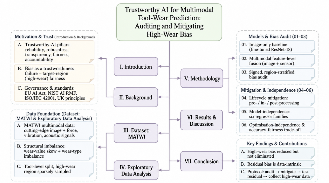
Figure 4.
The AI-enabled manufacturing stack, from shop-floor sensing to human decision. Trust must be maintained at every layer; this paper focuses on the AI model layer.
Figure 4.
The AI-enabled manufacturing stack, from shop-floor sensing to human decision. Trust must be maintained at every layer; this paper focuses on the AI model layer.
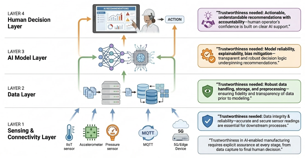
Figure 5.
The core pillars of trustworthy AI. The pillars are interdependent: a deficiency in any one undermines the trustworthiness of the whole.
Figure 5.
The core pillars of trustworthy AI. The pillars are interdependent: a deficiency in any one undermines the trustworthiness of the whole.
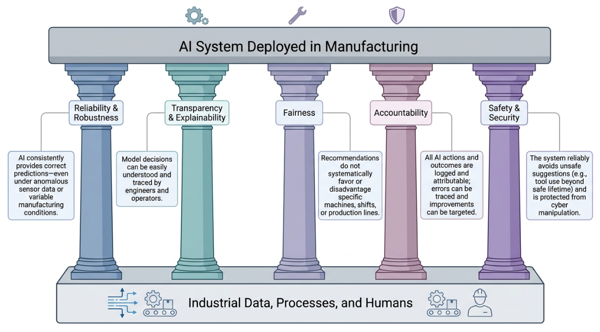
Figure 6.
Sources of bias across the machine-learning lifecycle. Because bias can enter at several stages, mitigation must likewise act at several stages — the rationale for the lifecycle pipeline introduced in the Introduction.
Figure 6.
Sources of bias across the machine-learning lifecycle. Because bias can enter at several stages, mitigation must likewise act at several stages — the rationale for the lifecycle pipeline introduced in the Introduction.
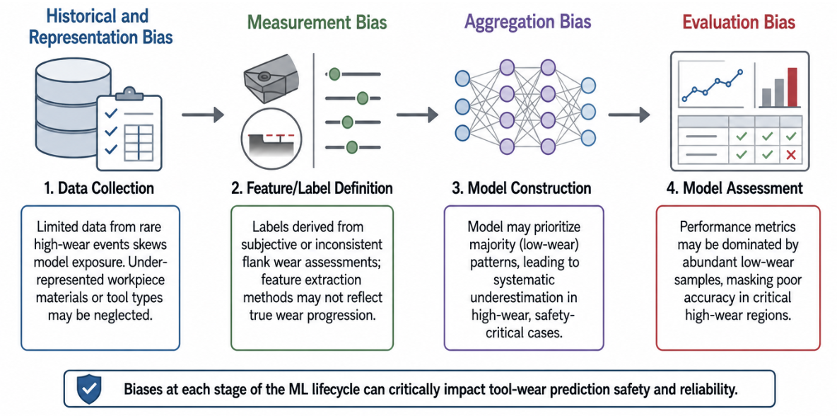
Figure 7.
The MATWI multimodal acquisition setup. Each milling pass produces one cutting-edge image and one synchronised multi-channel sensor recording.[12]
Figure 7.
The MATWI multimodal acquisition setup. Each milling pass produces one cutting-edge image and one synchronised multi-channel sensor recording.[12]
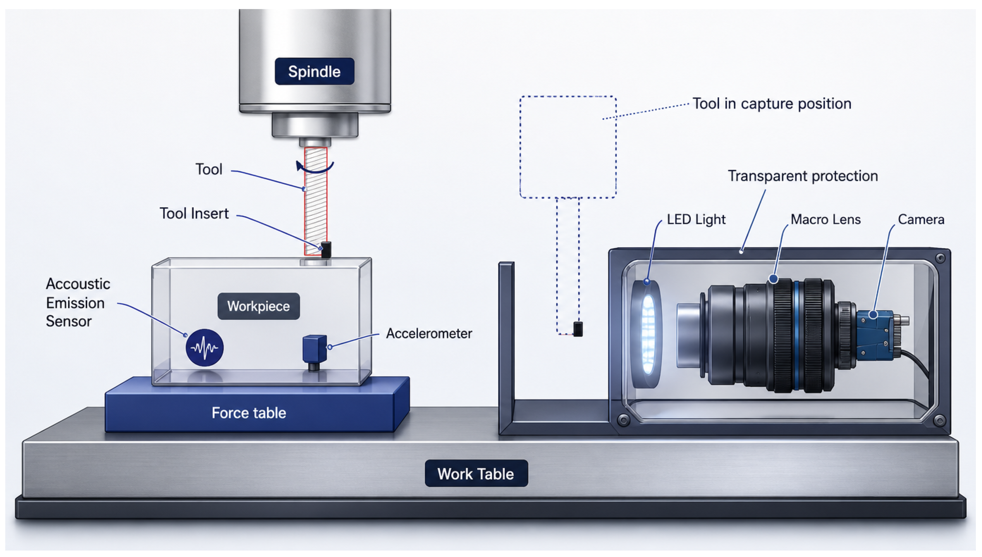
Figure 8.
A representative MATWI cutting-edge image ( pixels, RGB). The worn flank occupies only part of the frame; the remainder is background. Source: MATWI dataset [12].
Figure 8.
A representative MATWI cutting-edge image ( pixels, RGB). The worn flank occupies only part of the frame; the remainder is background. Source: MATWI dataset [12].
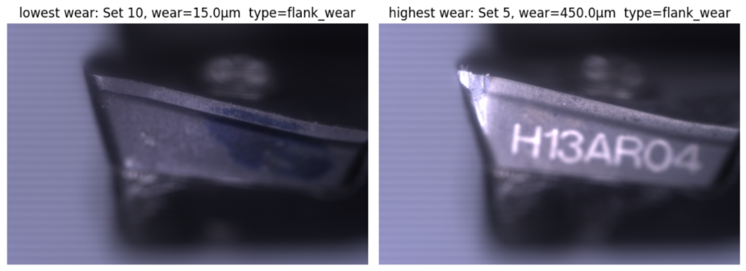
Figure 9.
The five sensor channels of one representative cut. The recordings are headerless and variable in length; channel activity is not uniform across all cuts, a property examined in Section 4.
Figure 9.
The five sensor channels of one representative cut. The recordings are headerless and variable in length; channel activity is not uniform across all cuts, a property examined in Section 4.
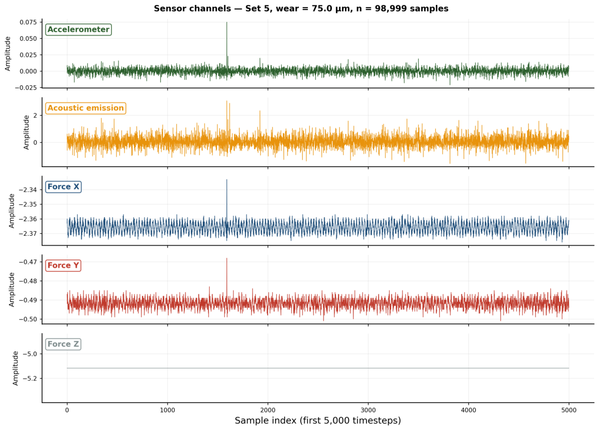
Figure 10.
Composition of the training, validation, and test partitions. The panels show the number of cuts of each workpiece material, the proportion of each wear type, the distribution of wear values, and the wear range covered by each constituent tool. Partitions are formed at the level of whole tools to prevent leakage of near-identical cuts.
Figure 10.
Composition of the training, validation, and test partitions. The panels show the number of cuts of each workpiece material, the proportion of each wear type, the distribution of wear values, and the wear range covered by each constituent tool. Partitions are formed at the level of whole tools to prevent leakage of near-identical cuts.
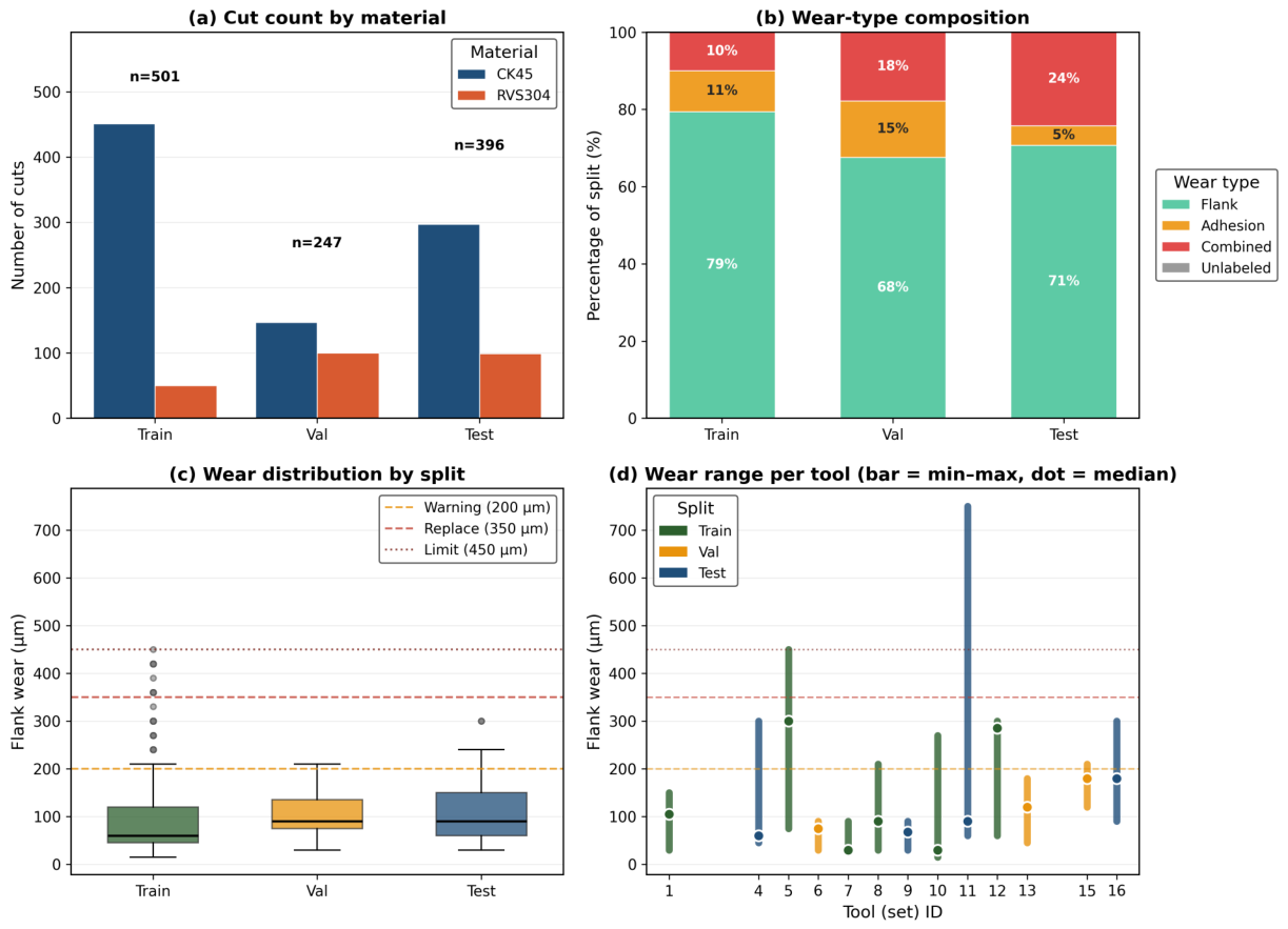
Figure 11.
Missing-data analysis across all seventeen tools. (a) Number of cuts per tool lacking an image, a sensor recording, or a wear-type label; incompleteness is concentrated in specific tools, reflecting indirect synchronisation between the camera and the CNC machine. (b) Usable-data percentage per tool; orange bars fall below the 80% threshold. (c) Global summary: of 1,803 raw rows, 1,566 pass the per-cut usability filter. (d) Force-channel activity rate per tool (fraction of cuts in which all three force axes are active). This panel makes the tool-level exclusion criterion explicit: Sets 2, 3, and 17 show pervasive force-channel inactivity across their entire tool run and are excluded at the tool level; Set 14 is excluded for a different reason (pilot run) and its channel activity is unaffected. Set 6, which appears elevated in panel (a) due to missing wear-type labels, is retained: its force-channel anomaly affects only individual cuts rather than the entire tool run, and those cuts are removed by the per-cut filter. The distinction between tool-level exclusion (Sets 2, 3, 14, 17) and cut-level removal (Set 6) is the operative curation criterion (Panel (c) reports 1,570 usable cuts. The verified count used throughout the paper is 1,566 (Table 5); the four-cut difference arises because the exploratory-analysis filter and the feature-extraction pipeline applied a slightly different file-existence check. The authoritative figure is 1,566.).
Figure 11.
Missing-data analysis across all seventeen tools. (a) Number of cuts per tool lacking an image, a sensor recording, or a wear-type label; incompleteness is concentrated in specific tools, reflecting indirect synchronisation between the camera and the CNC machine. (b) Usable-data percentage per tool; orange bars fall below the 80% threshold. (c) Global summary: of 1,803 raw rows, 1,566 pass the per-cut usability filter. (d) Force-channel activity rate per tool (fraction of cuts in which all three force axes are active). This panel makes the tool-level exclusion criterion explicit: Sets 2, 3, and 17 show pervasive force-channel inactivity across their entire tool run and are excluded at the tool level; Set 14 is excluded for a different reason (pilot run) and its channel activity is unaffected. Set 6, which appears elevated in panel (a) due to missing wear-type labels, is retained: its force-channel anomaly affects only individual cuts rather than the entire tool run, and those cuts are removed by the per-cut filter. The distinction between tool-level exclusion (Sets 2, 3, 14, 17) and cut-level removal (Set 6) is the operative curation criterion (Panel (c) reports 1,570 usable cuts. The verified count used throughout the paper is 1,566 (Table 5); the four-cut difference arises because the exploratory-analysis filter and the feature-extraction pipeline applied a slightly different file-existence check. The authoritative figure is 1,566.).
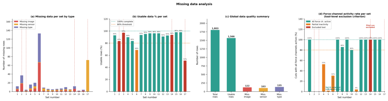
Figure 12.
Distribution of flank wear. The histogram and box plot both show a pronounced skew toward low wear, with the high-wear region sparsely populated in every partition. This imbalance is the structural cause of high-wear underestimation.
Figure 12.
Distribution of flank wear. The histogram and box plot both show a pronounced skew toward low wear, with the high-wear region sparsely populated in every partition. This imbalance is the structural cause of high-wear underestimation.
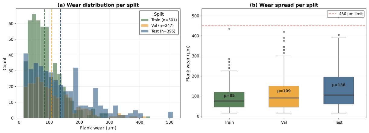
Figure 13.
Per-tool wear coverage. (a, top) Mean, maximum, and variability of wear for each tool; (b, bottom) the wear range traversed by each tool. Most tools remain in the low-wear region; only Set 5 spans the full range and only Set 11 exceeds it. High-wear data is concentrated in very few tools.
Figure 13.
Per-tool wear coverage. (a, top) Mean, maximum, and variability of wear for each tool; (b, bottom) the wear range traversed by each tool. Most tools remain in the low-wear region; only Set 5 spans the full range and only Set 11 exceeds it. High-wear data is concentrated in very few tools.
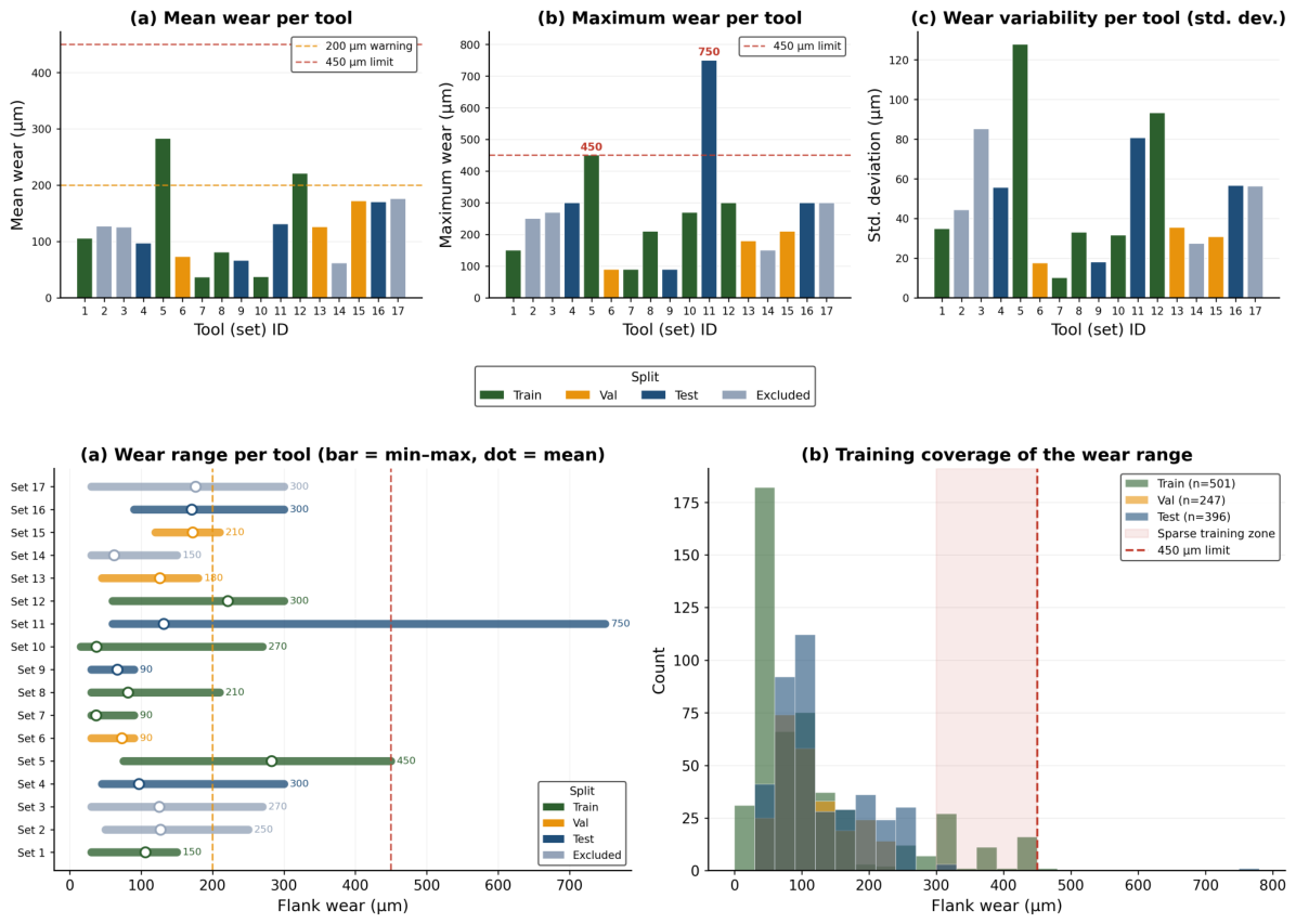
Figure 14.
Wear-type composition. (top) Wear type per tool; (bottom) overall, per-partition, and per-material proportions. Flank wear dominates overall (68.6%), with combined wear (20.1%) and adhesive wear (11.3%) less common and unevenly distributed across tools and materials, giving a second axis of imbalance independent of the wear-value skew.
Figure 14.
Wear-type composition. (top) Wear type per tool; (bottom) overall, per-partition, and per-material proportions. Flank wear dominates overall (68.6%), with combined wear (20.1%) and adhesive wear (11.3%) less common and unevenly distributed across tools and materials, giving a second axis of imbalance independent of the wear-value skew.
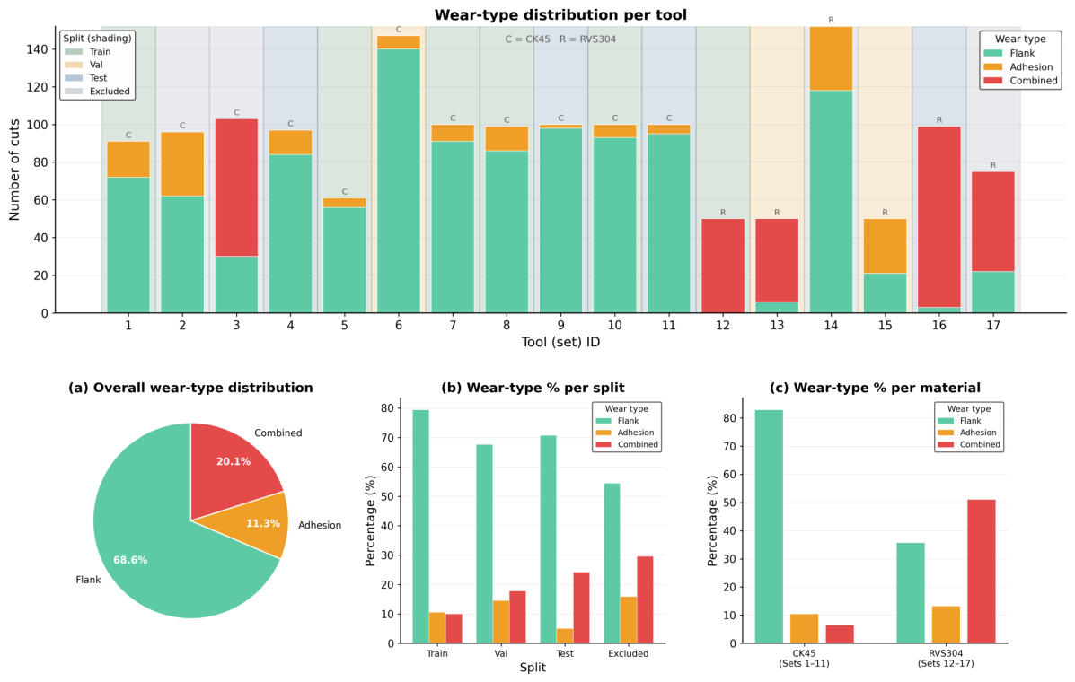
Figure 15.
Flank wear against cutting parameters. At any fixed parameter value the wear spans a wide range, showing that the controlled settings alone do not determine wear and cannot serve as sufficient predictors.
Figure 15.
Flank wear against cutting parameters. At any fixed parameter value the wear spans a wide range, showing that the controlled settings alone do not determine wear and cannot serve as sufficient predictors.
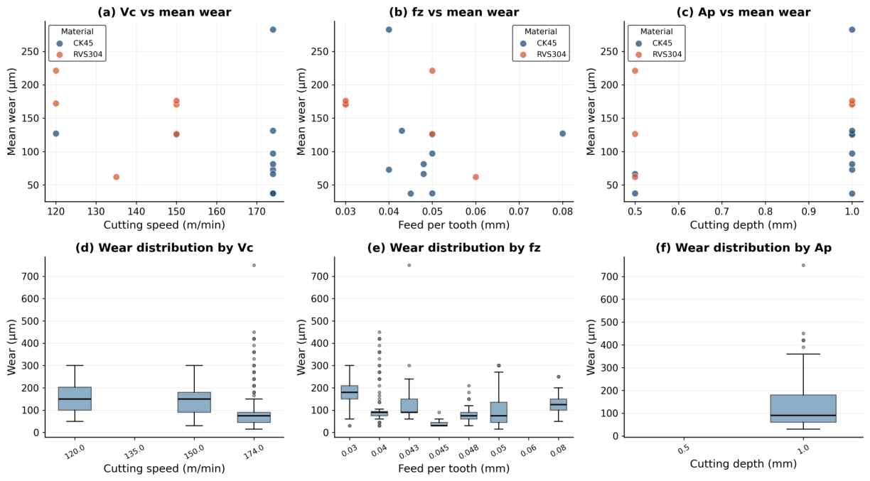
Figure 16.
Per-channel sensor statistics across tools. The five channels’ distributions vary systematically between tools, indicating that the sensor signals carry wear-relevant information. One force channel is inactive in a substantial minority of cuts.
Figure 16.
Per-channel sensor statistics across tools. The five channels’ distributions vary systematically between tools, indicating that the sensor signals carry wear-relevant information. One force channel is inactive in a substantial minority of cuts.
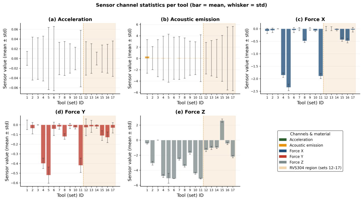
Figure 17.
Sensor-derived features against wear. Several extracted features correlate with the wear value, confirming the sensor modality carries genuine predictive signal, though the associations are only moderate and some channels are incomplete.
Figure 17.
Sensor-derived features against wear. Several extracted features correlate with the wear value, confirming the sensor modality carries genuine predictive signal, though the associations are only moderate and some channels are incomplete.
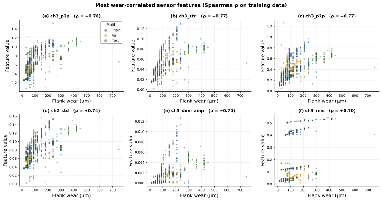
Figure 18.
Visual content of the cutting-edge images. Representative images and a comparison of the average low-wear and high-wear appearance reveal a consistent, physically interpretable visual signature of wear, establishing the image modality as a strong direct predictor.
Figure 18.
Visual content of the cutting-edge images. Representative images and a comparison of the average low-wear and high-wear appearance reveal a consistent, physically interpretable visual signature of wear, establishing the image modality as a strong direct predictor.
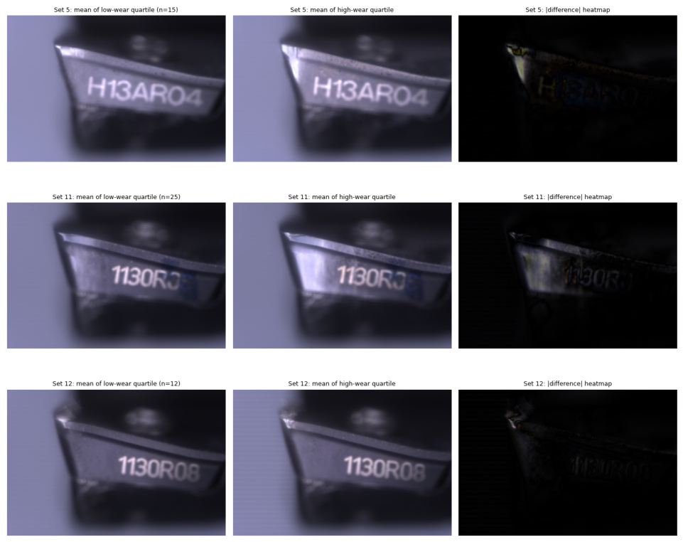
Figure 19.
Overview of the methodology. Band A builds the multimodal model (Objectives 1–2): data preparation, the image and sensor feature branches, 596-d feature-level fusion, and the dual-output Model 2. Band B is the trustworthy-AI programme (Objectives 3–6): the signed bias audit, the three-stage (pre/in/post) lifecycle mitigation yielding Model 3, and the model- and optimisation-independence tests, converging on the data-intrinsic finding.
Figure 19.
Overview of the methodology. Band A builds the multimodal model (Objectives 1–2): data preparation, the image and sensor feature branches, 596-d feature-level fusion, and the dual-output Model 2. Band B is the trustworthy-AI programme (Objectives 3–6): the signed bias audit, the three-stage (pre/in/post) lifecycle mitigation yielding Model 3, and the model- and optimisation-independence tests, converging on the data-intrinsic finding.
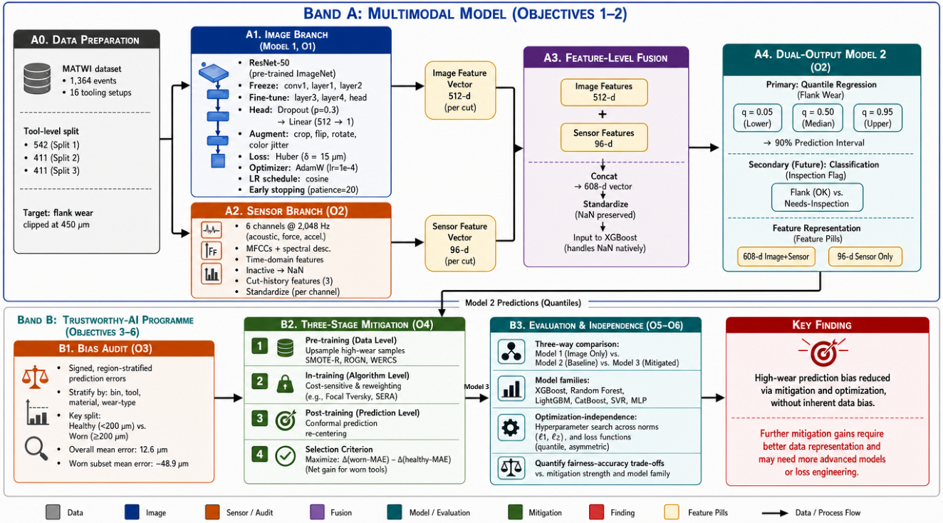
Figure 20.
The image-only baseline. A cutting-edge image is augmented and passed through a partially fine-tuned ResNet-18 (early stages frozen, deeper blocks trainable); the global average-pooling layer feeds a dropout-and-linear head that regresses a scalar wear value. The dashed path shows the training-time loss and gradient update (Huber loss, AdamW, cosine schedule, early stopping), which are inactive at inference.
Figure 20.
The image-only baseline. A cutting-edge image is augmented and passed through a partially fine-tuned ResNet-18 (early stages frozen, deeper blocks trainable); the global average-pooling layer feeds a dropout-and-linear head that regresses a scalar wear value. The dashed path shows the training-time loss and gradient update (Huber loss, AdamW, cosine schedule, early stopping), which are inactive at inference.
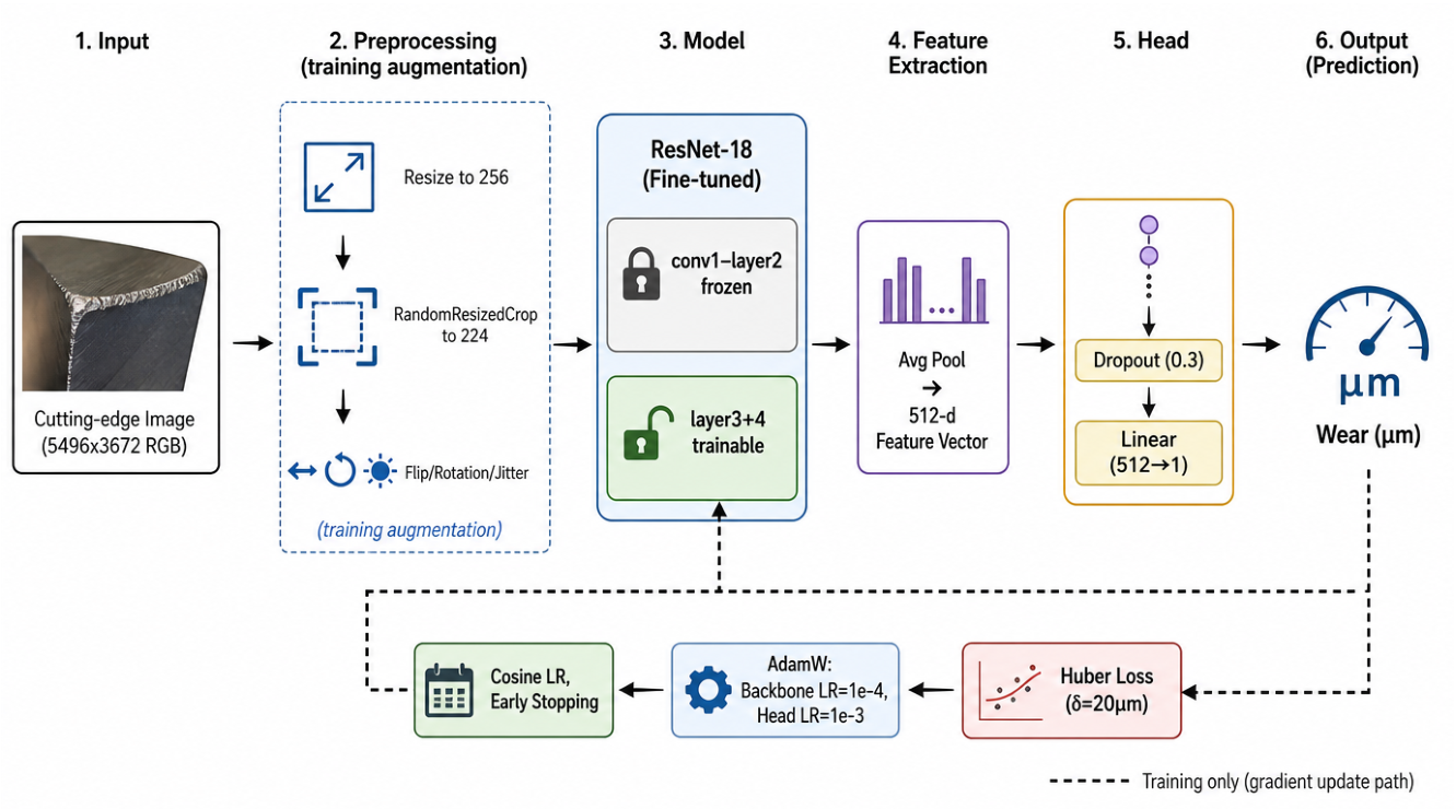
Figure 21.
The multimodal feature-level fusion architecture. The image branch (a fine-tuned ResNet-18) and the sensor branch (hand-crafted signal-processing features) each encode one cut into a fixed-length vector; the two are concatenated and standardised, and gradient-boosted models produce a wear estimate with a prediction interval and a wear-type inspection flag.
Figure 21.
The multimodal feature-level fusion architecture. The image branch (a fine-tuned ResNet-18) and the sensor branch (hand-crafted signal-processing features) each encode one cut into a fixed-length vector; the two are concatenated and standardised, and gradient-boosted models produce a wear estimate with a prediction interval and a wear-type inspection flag.
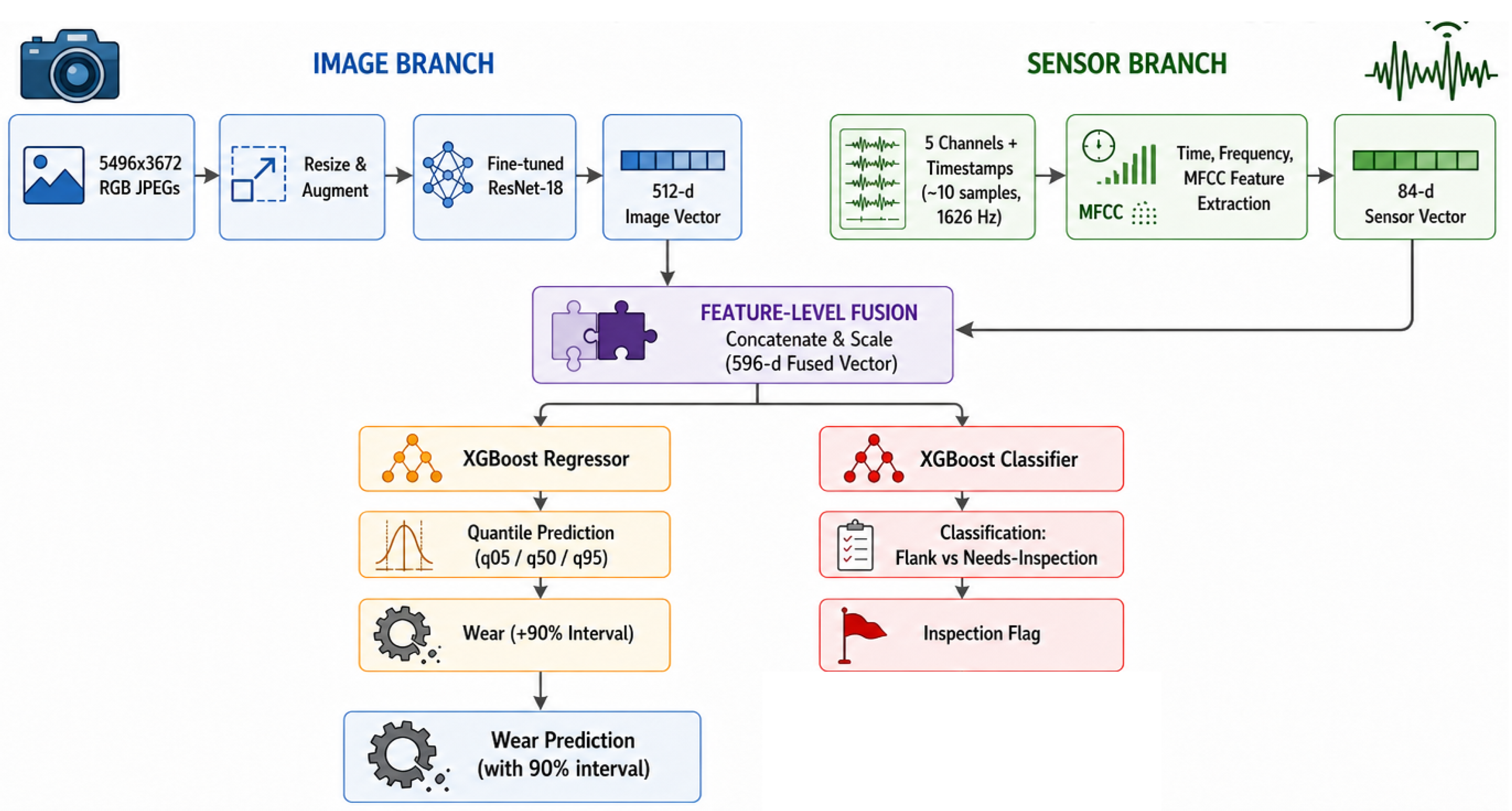
Figure 22.
Training trajectory of the image-only ResNet-18. Validation error falls steeply for the first six epochs and reaches its minimum of (the saved checkpoint), after which the two curves diverge: the training MAE continues to fall while the validation MAE rises, the standard signature of overfitting. Early stopping terminates training at epoch fourteen.
Figure 22.
Training trajectory of the image-only ResNet-18. Validation error falls steeply for the first six epochs and reaches its minimum of (the saved checkpoint), after which the two curves diverge: the training MAE continues to fall while the validation MAE rises, the standard signature of overfitting. Early stopping terminates training at epoch fourteen.
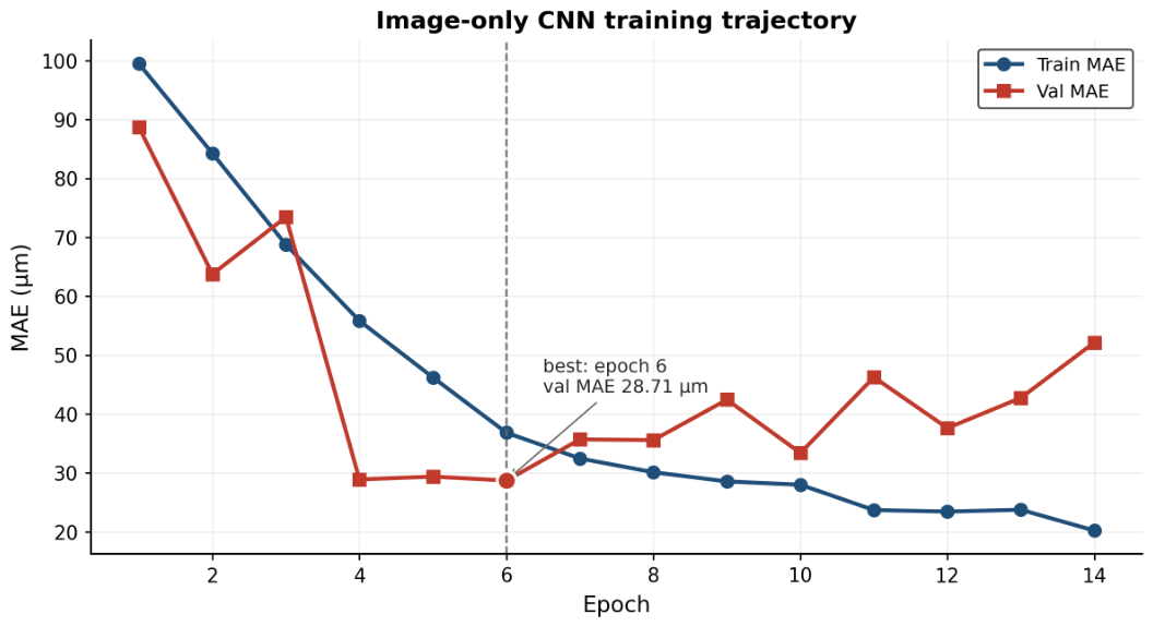
Figure 23.
Distribution of the per-feature Spearman correlation with wear, computed over the 512 ResNet activations on the training split. The entire distribution lies in the positive region; the median (dashed line) sits at and the range spans to . Every image feature individually tracks wear, consistent with the network having learned a wear-monotonic representation.
Figure 23.
Distribution of the per-feature Spearman correlation with wear, computed over the 512 ResNet activations on the training split. The entire distribution lies in the positive region; the median (dashed line) sits at and the range spans to . Every image feature individually tracks wear, consistent with the network having learned a wear-monotonic representation.
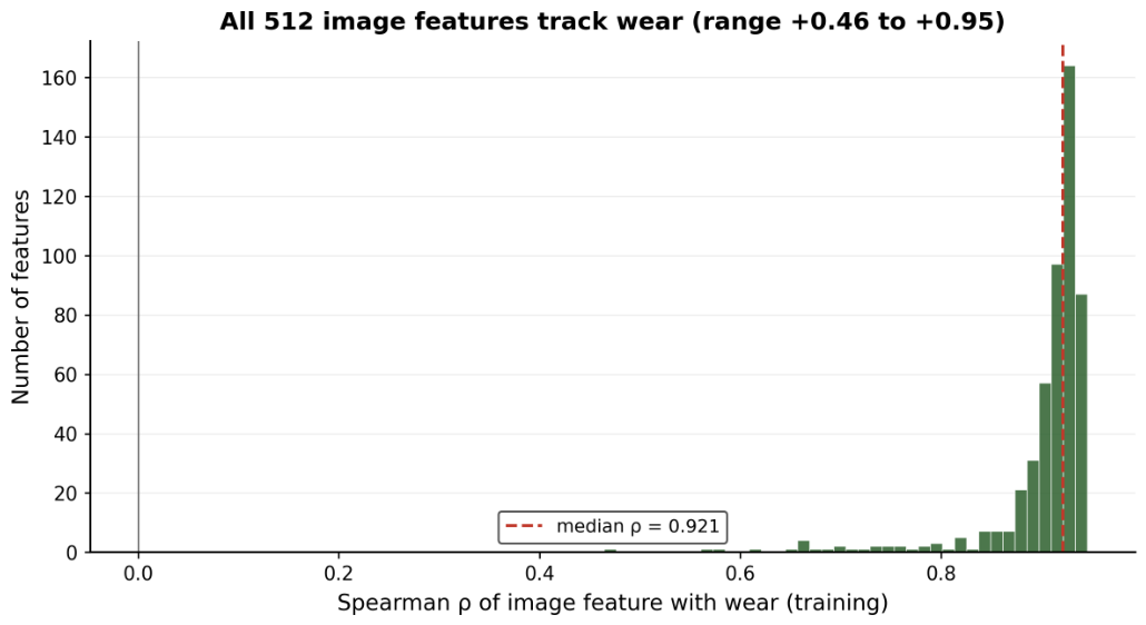
Figure 24.
Test mean absolute error by wear bin for the three models. The number of test cuts (n) above each bin shows how sharply the data thins towards higher wear. The image-only baseline (red) rises from 14 to almost across the bins; the fusion model (green) reduces the error decisively in the operational middle of the range but still degrades in the sparsely populated upper bins.
Figure 24.
Test mean absolute error by wear bin for the three models. The number of test cuts (n) above each bin shows how sharply the data thins towards higher wear. The image-only baseline (red) rises from 14 to almost across the bins; the fusion model (green) reduces the error decisively in the operational middle of the range but still degrades in the sparsely populated upper bins.
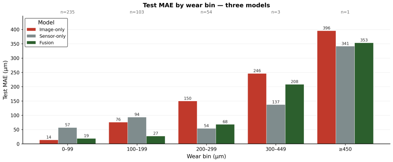
Figure 25.
Predicted against true wear for the image-only baseline on each split, with points coloured by tool. The training and validation panels follow the perfect-prediction diagonal reasonably; on the test panel the predictions collapse to a near-horizontal band, reflecting the model’s inability to extrapolate to high wear on tools it has not seen during training. The dotted red lines mark the operational decision boundary.
Figure 25.
Predicted against true wear for the image-only baseline on each split, with points coloured by tool. The training and validation panels follow the perfect-prediction diagonal reasonably; on the test panel the predictions collapse to a near-horizontal band, reflecting the model’s inability to extrapolate to high wear on tools it has not seen during training. The dotted red lines mark the operational decision boundary.
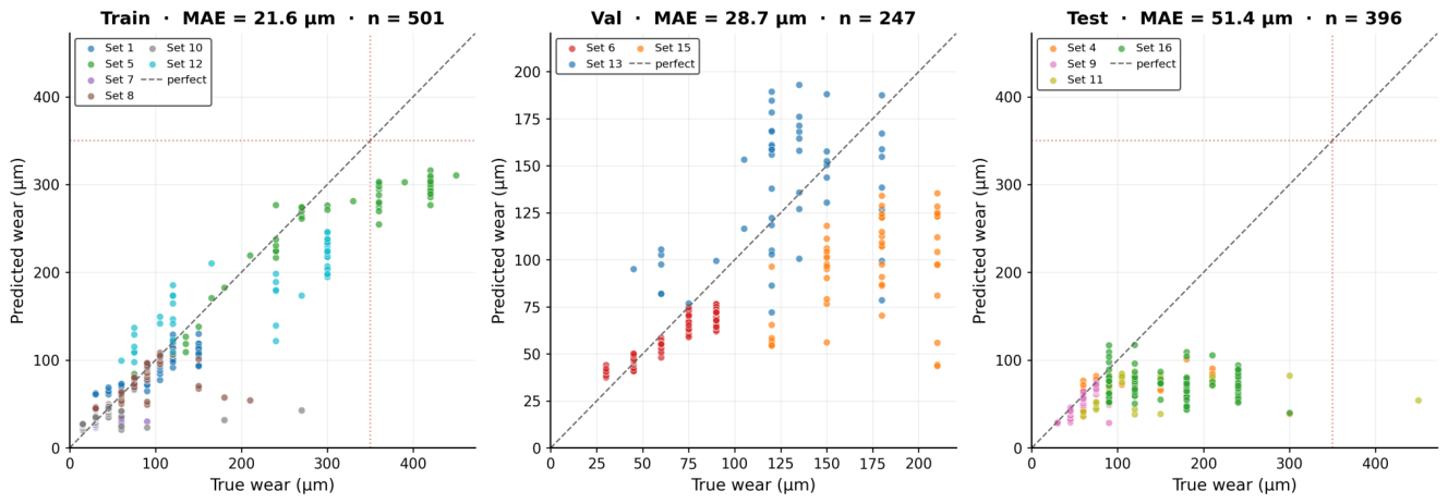
Figure 26.
Predicted against true wear on the test split for the three models. The image-only baseline (left) saturates at low predicted values irrespective of the true wear, the sensor-only model (centre) is noisier and over-predicts low wear, and the multimodal fusion (right) follows the diagonal substantially more closely across the whole range.
Figure 26.
Predicted against true wear on the test split for the three models. The image-only baseline (left) saturates at low predicted values irrespective of the true wear, the sensor-only model (centre) is noisier and over-predicts low wear, and the multimodal fusion (right) follows the diagonal substantially more closely across the whole range.
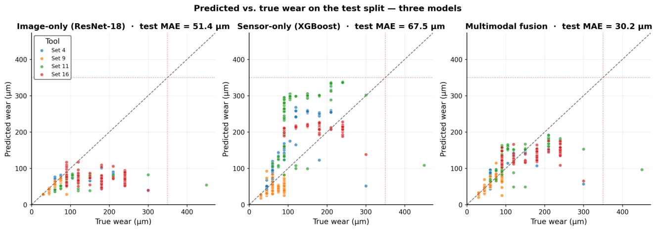
Figure 27.
Empirical coverage of the prediction interval on the test split, by wear bin. The dashed line marks the nominal target; the mean interval width is annotated above each bar. The interval is conservatively calibrated up to the 300– bin but collapses to zero coverage on the single cut, where the true wear lies entirely above the predicted upper bound.
Figure 27.
Empirical coverage of the prediction interval on the test split, by wear bin. The dashed line marks the nominal target; the mean interval width is annotated above each bar. The interval is conservatively calibrated up to the 300– bin but collapses to zero coverage on the single cut, where the true wear lies entirely above the predicted upper bound.
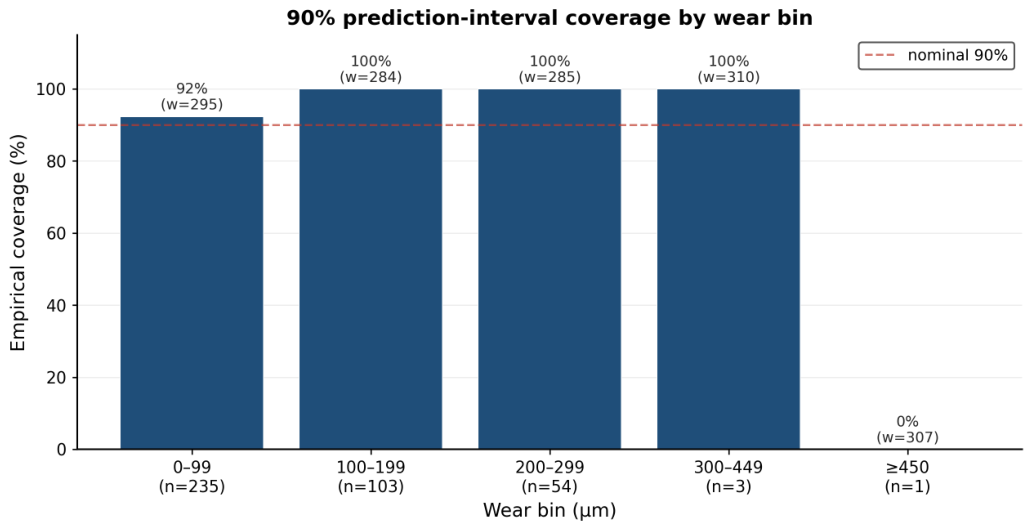
Figure 28.
Test-split confusion matrix of the three-class wear-type classifier. The matrix is overwhelmingly concentrated in the flank column: every adhesion case is predicted as flank, every combined case is predicted as flank, and only one true-flank case is misclassified. The result is the headline accuracy of , achieved entirely through majority-class collapse and providing no useful diagnostic information on the minority classes.
Figure 28.
Test-split confusion matrix of the three-class wear-type classifier. The matrix is overwhelmingly concentrated in the flank column: every adhesion case is predicted as flank, every combined case is predicted as flank, and only one true-flank case is misclassified. The result is the headline accuracy of , achieved entirely through majority-class collapse and providing no useful diagnostic information on the minority classes.
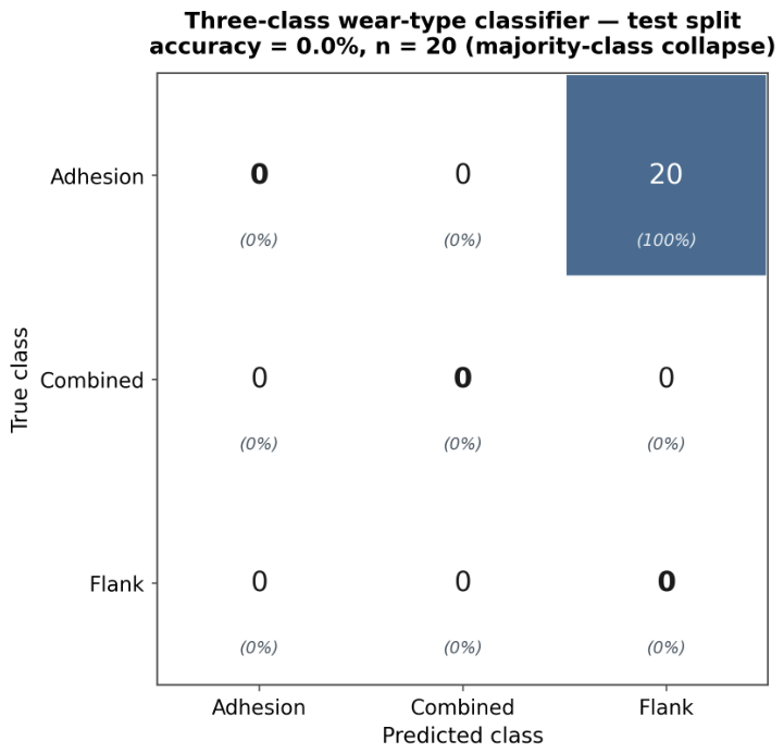
Figure 29.
Inspection-classifier behaviour on the test split. (a) Recall, precision, and false-alarm rate as a function of the decision threshold; the dashed vertical marks the selected operating point at . (b) The five test operating points in the false-alarm/recall plane, with their thresholds labelled. The full ROC area under the curve, computed over all thresholds, is .
Figure 29.
Inspection-classifier behaviour on the test split. (a) Recall, precision, and false-alarm rate as a function of the decision threshold; the dashed vertical marks the selected operating point at . (b) The five test operating points in the false-alarm/recall plane, with their thresholds labelled. The full ROC area under the curve, computed over all thresholds, is .
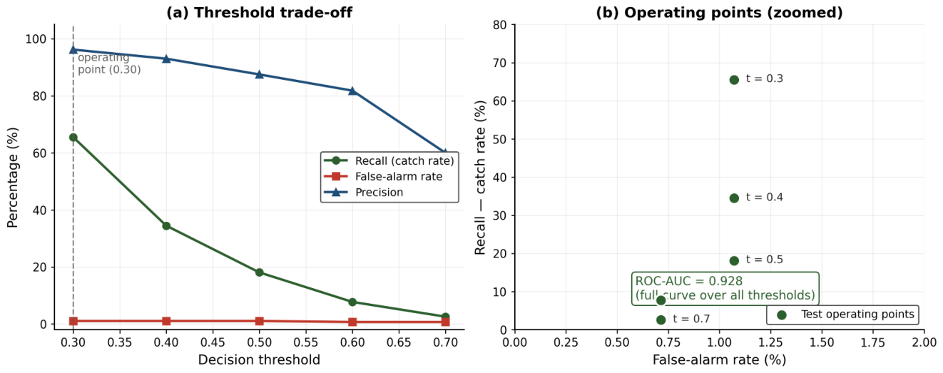
Figure 30.
Test-split confusion matrices of the binary classifier at two decision thresholds. (a) At the default threshold , the classifier flags only 21 of 116 inspection cases ( recall) with a near-zero false-alarm rate. (b) Lowering the threshold to the selected operating point raises the catch rate to 76 of 116 () while leaving the false-alarm count at 3 ( false-alarm rate). The change in threshold trades a fivefold increase in recall for almost no change in precision ().
Figure 30.
Test-split confusion matrices of the binary classifier at two decision thresholds. (a) At the default threshold , the classifier flags only 21 of 116 inspection cases ( recall) with a near-zero false-alarm rate. (b) Lowering the threshold to the selected operating point raises the catch rate to 76 of 116 () while leaving the false-alarm count at 3 ( false-alarm rate). The change in threshold trades a fivefold increase in recall for almost no change in precision ().
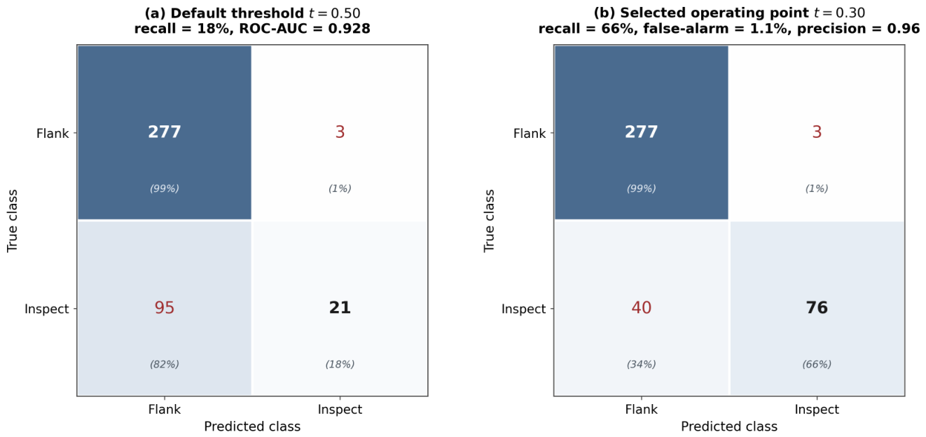
Figure 31.
Bias audit of the multimodal model. (a) Test-set wear distribution (bars) with per-bin MAE (line): error grows where data is scarce. (b) Predicted versus true wear by test tool, showing saturation at high wear. (c) Signed per-bin error, deepening monotonically with wear; sample counts annotated. (d) MAE per wear window against the sample count per window, showing that the largest errors coincide with the sparsest, highest-wear regions.
Figure 31.
Bias audit of the multimodal model. (a) Test-set wear distribution (bars) with per-bin MAE (line): error grows where data is scarce. (b) Predicted versus true wear by test tool, showing saturation at high wear. (c) Signed per-bin error, deepening monotonically with wear; sample counts annotated. (d) MAE per wear window against the sample count per window, showing that the largest errors coincide with the sparsest, highest-wear regions.
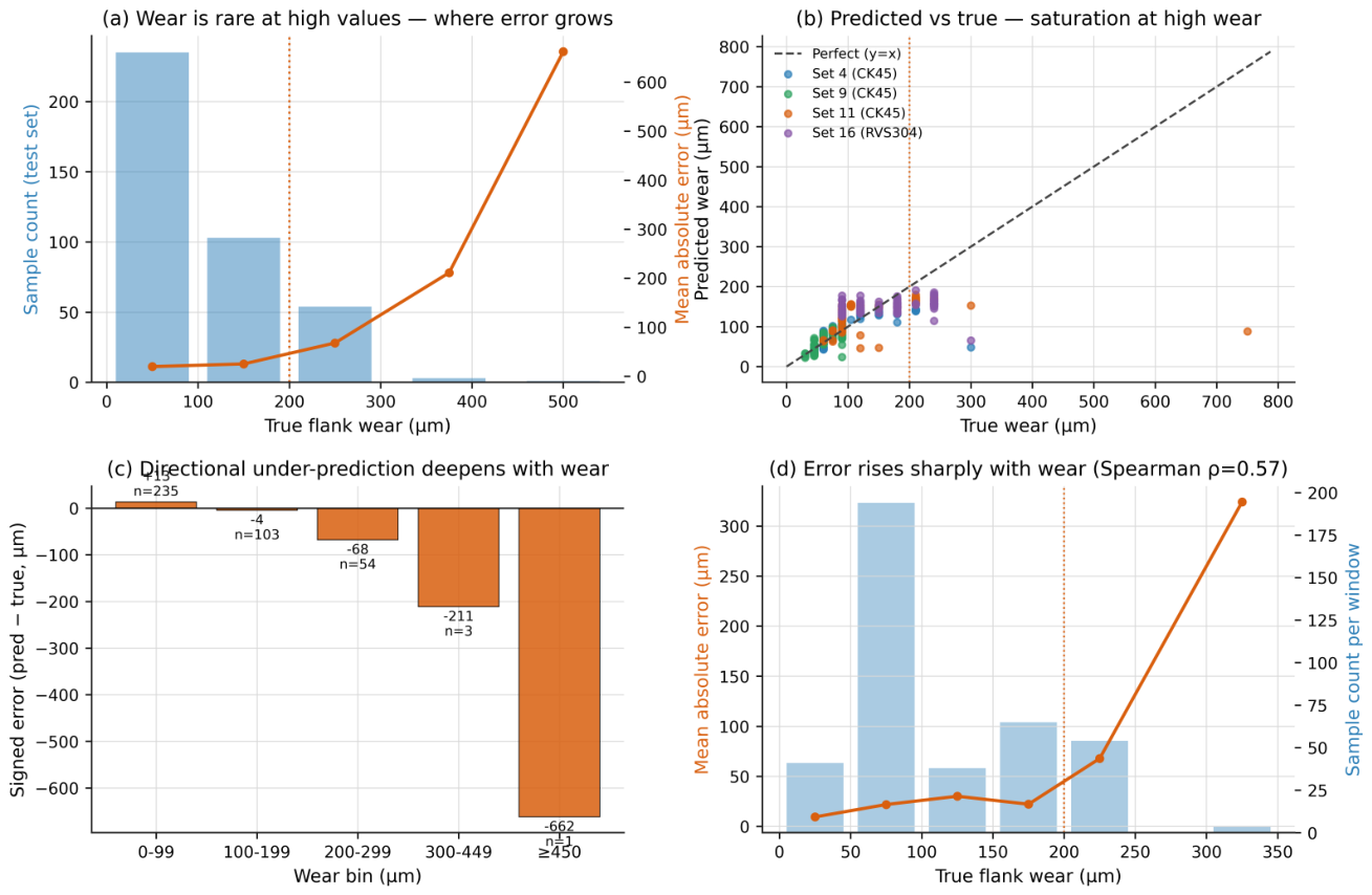
Figure 32.
Three-way comparison. (a) Per-bin signed error for the multimodal (Model 2) and mitigated (Model 3) models: mitigation lifts predictions across the range, easing the high-wear under-prediction while over-shooting the well-sampled low-wear bins. (b) Aggregate and worn-region MAE for the three models, showing that fusion reduces error and mitigation trades overall accuracy for a smaller worn-region error.
Figure 32.
Three-way comparison. (a) Per-bin signed error for the multimodal (Model 2) and mitigated (Model 3) models: mitigation lifts predictions across the range, easing the high-wear under-prediction while over-shooting the well-sampled low-wear bins. (b) Aggregate and worn-region MAE for the three models, showing that fusion reduces error and mitigation trades overall accuracy for a smaller worn-region error.
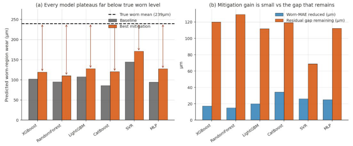
Figure 33.
Model-independence of the residual high-wear bias. For each of six regressor families, the predicted worn-region wear under the baseline and under the family’s own best mitigation is shown against the true worn level (dashed). Every family plateaus far below the true level, and mitigation moves each only marginally toward it.
Figure 33.
Model-independence of the residual high-wear bias. For each of six regressor families, the predicted worn-region wear under the baseline and under the family’s own best mitigation is shown against the true worn level (dashed). Every family plateaus far below the true level, and mitigation moves each only marginally toward it.
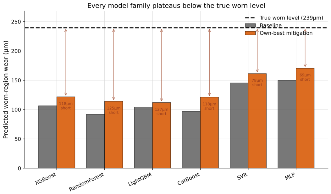
Table 1.
Positioning of this work relative to representative studies on data-driven tool-wear prediction and trustworthy industrial AI. A check mark (✓) indicates that the capability is a stated focus of the work, and a cross (×) that it is not addressed; the marks characterise scope rather than quality.
Table 1.
Positioning of this work relative to representative studies on data-driven tool-wear prediction and trustworthy industrial AI. A check mark (✓) indicates that the capability is a stated focus of the work, and a cross (×) that it is not addressed; the marks characterise scope rather than quality.
| Capability | [12] | [21] | [15] | This Work |
|---|---|---|---|---|
| Multimodal fusion (image + process sensors) | × | × | × | ✓ |
| Tool-wear regression (continuous target) | ✓ | ✓ | × | ✓ |
| Signed, region-stratified bias audit | × | × | × | ✓ |
| Lifecycle (pre/in/post) mitigation | × | × | ✓ | ✓ |
| Target-region fairness evaluation of regression | × | × | × | ✓ |
| Model-independence test (multiple families) | × | × | ✓ | ✓ |
| Optimisation-independence test (tuning + losses) | × | × | × | ✓ |
| Data-intrinsic characterisation of residual bias | × | × | × | ✓ |
Table 2.
How major AI-governance frameworks and standards define fairness. Despite differing in legal form, all converge on the avoidance of unjust bias and discrimination as a core requirement of trustworthy AI.
Table 2.
How major AI-governance frameworks and standards define fairness. Despite differing in legal form, all converge on the avoidance of unjust bias and discrimination as a core requirement of trustworthy AI.
| Source / Instrument | Treatment of fairness | Emphasis |
|---|---|---|
| ISO/IEC TR 24028:2020 | Fairness as the avoidance of unjust discrimination and bias, as part of AI trustworthiness | Standards-based trustworthiness |
| ISO/IEC 42001:2023 | Management-system controls for transparency, fairness, and bias risk across the AI lifecycle | Auditable organisational governance |
| OECD AI Principles (2019, upd. 2024) | AI systems should avoid unfair bias and discrimination against individuals or groups | Inclusive growth, policy alignment |
| IEEE Ethically Aligned Design | AI should be designed to avoid unjustified bias and to promote fairness and inclusivity | Engineering ethics |
| EU AI Act (Reg. (EU) 2024/1689) | Binding data-quality and risk-management duties to limit bias in high-risk systems | Prescriptive, risk-based regulation |
| NIST AI RMF (2023) | “Fair with harmful bias managed” listed as a core trustworthiness characteristic | Voluntary risk-management framework |
| China — AI Governance Principles (2019) | AI should promote fairness and inclusiveness and avoid discrimination | State-guided ethical governance |
| India — Responsible AI for All (NITI Aayog, 2021) | AI must prevent bias and ensure equitable, inclusive access | Inclusive national AI growth |
| UK — Pro-Innovation Approach (2023) | Fairness as one of five cross-sector regulatory principles | Principles-based, sector-led |
Table 4.
Per-set wear characteristics of the seventeen MATWI tools, as measured in this study. Tools 1–11 use CK45 steel; tools 12–17 use RVS 304 stainless steel. Wear values are in micrometres.
Table 4.
Per-set wear characteristics of the seventeen MATWI tools, as measured in this study. Tools 1–11 use CK45 steel; tools 12–17 use RVS 304 stainless steel. Wear values are in micrometres.
| Set | Material | Cuts | Min | Max | Mean | Median | Reaches 450 |
|---|---|---|---|---|---|---|---|
| 1 | CK45 | 91 | 30 | 150 | 105.8 | 105.0 | No |
| 2 | CK45 | 96 | 50 | 250 | 127.1 | 125.0 | No |
| 3 | CK45 | 103 | 30 | 270 | 125.4 | 90.0 | No |
| 4 | CK45 | 97 | 45 | 300 | 97.0 | 60.0 | No |
| 5 | CK45 | 61 | 75 | 450 | 282.8 | 300.0 | Yes |
| 6 | CK45 | 147 | 30 | 90 | 73.0 | 75.0 | No |
| 7 | CK45 | 100 | 30 | 90 | 37.0 | 30.0 | No |
| 8 | CK45 | 99 | 30 | 210 | 81.4 | 90.0 | No |
| 9 | CK45 | 100 | 30 | 90 | 66.6 | 67.5 | No |
| 10 | CK45 | 100 | 15 | 270 | 37.5 | 30.0 | No |
| 11 | CK45 | 100 | 60 | 750 | 131.4 | 90.0 | Yes |
| 12 | RVS304 | 50 | 60 | 300 | 221.1 | 285.0 | No |
| 13 | RVS304 | 50 | 45 | 180 | 126.3 | 120.0 | No |
| 14 | RVS304 | 152 | 30 | 150 | 61.9 | 60.0 | No |
| 15 | RVS304 | 50 | 120 | 210 | 172.2 | 180.0 | No |
| 16 | RVS304 | 99 | 90 | 300 | 170.6 | 180.0 | No |
| 17 | RVS304 | 75 | 30 | 300 | 176.0 | 180.0 | No |
Table 5.
Cut-level accounting from raw index to modelling corpus. Two sequential curation steps reduce the 1,803-row raw index to the 1,144 cuts used for modelling.
Table 5.
Cut-level accounting from raw index to modelling corpus. Two sequential curation steps reduce the 1,803-row raw index to the 1,144 cuts used for modelling.
| Stage | Cuts retained | Cuts removed |
|---|---|---|
| Raw rows in labels.csv | 1,803 | — |
| After per-cut usability filter | 1,566 | 237 |
| valid image + sensor recording + wear value | ||
| After tool-level exclusion | 1,144 | 422 |
| Sets 2 (96 cuts), 3 (103 cuts), 14 (148 cuts), 17 (75 cuts) | ||
| Training partition | 501 | — |
| Validation partition | 247 | — |
| Test partition | 396 | — |
Table 6.
Imbalanced-regression toolkit applied to the regression branch. Each method is appropriate for a continuous imbalanced target and preserves the wear signal; the framework column names the established toolkit and reference implementation. The collective outcome is a reduction, but not elimination, of the high-wear bias.
Table 6.
Imbalanced-regression toolkit applied to the regression branch. Each method is appropriate for a continuous imbalanced target and preserves the wear signal; the framework column names the established toolkit and reference implementation. The collective outcome is a reduction, but not elimination, of the high-wear bias.
| Method (Reference) | Stage | Framework / Toolkit | Mechanism | Outcome in This Study |
|---|---|---|---|---|
| SMOTER [39] | Pre | ImbalancedLearningRegression; SMOGN [41,45] | Synthesises rare high-wear samples by interpolating features and target between nearest neighbours | Rebalances training distribution; reduces but does not close the worn-region gap |
| ROGN (Gaussian-noise resampling) [41] | Pre | ImbalancedLearningRegression; SMOGN [41,45] | Oversamples rare high-wear cuts with added Gaussian perturbation to expand their support | Selected as the best pre-processing method on the documented model; partial worn-region gain |
| WERCS [42] | Pre | ImbalancedLearningRegression [45] | Combined probabilistic over- and under-sampling driven by a relevance function | Screened; competitive on some model families |
| Cost-sensitive wear-bin weighting | In | XGBoost (sample_weight) [46] | Weights high-wear cuts more heavily in the training loss | Conservative weighting is the documented Model 2 recipe; captures most achievable reduction at low cost |
| Relevance-based weighting (SERA-inspired) [43] | In | Relevance-based weighting (own implementation) | Increases the loss penalty continuously with target relevance (wear) | Selected as the best in-processing method; largest single-stage worn-region reduction |
| Conformal recentring [44] | Post | Conformal prediction (MAPIE) [44,47] | Recalibrates the upper wear range using split-conformal adjustment | Selected as the best post-processing method; small additional worn-region gain |
| SERA metric [43] | Measure | ImbalancedLearningRegression [43,45] | Error metric weighted toward rare target values | Used as the rare-target error metric throughout the regression arm |
Table 7.
Image-only baseline at the best-on-validation epoch. The training and validation errors are similar, but the test error is roughly larger, indicating that the test tools span operating conditions absent or under-represented in training.
Table 7.
Image-only baseline at the best-on-validation epoch. The training and validation errors are similar, but the test error is roughly larger, indicating that the test tools span operating conditions absent or under-represented in training.
| Split | n | MAE (m) | RMSE (m) |
|---|---|---|---|
| Train | 496 | 29.5 | 50.5 |
| Validation | 247 | 28.7 | 42.2 |
| Test | 396 | 51.4 | 77.1 |
Table 8.
Aggregate test-split performance of the two baselines and a single-modality sensor reference. The fused model improves on the better single-modality baseline by ().
Table 8.
Aggregate test-split performance of the two baselines and a single-modality sensor reference. The fused model improves on the better single-modality baseline by ().
| Model | Features | Test MAE (m) |
|---|---|---|
| Sensor-only (XGBoost) | 84 | 68.3 |
| Image-only (ResNet-18) | 512 | 51.4 |
| Multimodal fusion | 596 | 30.9 |
Table 9.
Test MAE by wear bin for the three models, with the mean prediction reported alongside the MAE for image-only and fusion (the column was not printed for sensor-only in the source notebook). The image-only model’s mean prediction in the four upper bins stays in a narrow range (54–m) even as the true wear rises to m, evidencing a saturating output. The fusion model corrects this substantially in the operational middle of the range but partially regresses in the sparsely populated upper bins. Bootstrap 95% confidence intervals (10,000 resamples) are given for each MAE; the interval is wide and indicative only, and the bin admits no interval.
Table 9.
Test MAE by wear bin for the three models, with the mean prediction reported alongside the MAE for image-only and fusion (the column was not printed for sensor-only in the source notebook). The image-only model’s mean prediction in the four upper bins stays in a narrow range (54–m) even as the true wear rises to m, evidencing a saturating output. The fusion model corrects this substantially in the operational middle of the range but partially regresses in the sparsely populated upper bins. Bootstrap 95% confidence intervals (10,000 resamples) are given for each MAE; the interval is wide and indicative only, and the bin admits no interval.
| Bin (m) | n | Image-only | Sensor-only | Fusion | ||||
|---|---|---|---|---|---|---|---|---|
| MAE | 95% CI | mean pred | MAE | MAE | 95% CI | mean pred | ||
| 0–99 | 235 | 14.1 | [13, 15] | 59.3 | 57.1 | 19.0 | [17, 22] | 83.1 |
| 100–199 | 103 | 75.9 | [69, 82] | 72.0 | 93.6 | 27.5 | [23, 32] | 136.2 |
| 200–299 | 54 | 149.9 | [144, 155] | 76.8 | 54.3 | 68.2 | [62, 75] | 158.5 |
| 300–449 | 3 | 246.4 | [218, 261] | 53.6 | 137.2 | 208.2 | [147, 243] | 91.8 |
| ≥450 | 1 | 395.7 | — | 54.3 | 341.5 | 353.5 | — | 96.5 |
Table 10.
Per-tool performance on the test split. The signed-bias column for the image-only model is the mean prediction minus the mean target; every entry is negative, indicating that the image-only model never systematically over-estimates. The largest under-estimations are on the two tools that reach the high-wear region (Sets 11 and 16). The fusion improves on the image-only model on three of the four test tools but matches it on Set 9, which is the easiest (low-wear) tool.
Table 10.
Per-tool performance on the test split. The signed-bias column for the image-only model is the mean prediction minus the mean target; every entry is negative, indicating that the image-only model never systematically over-estimates. The largest under-estimations are on the two tools that reach the high-wear region (Sets 11 and 16). The fusion improves on the image-only model on three of the four test tools but matches it on Set 9, which is the easiest (low-wear) tool.
| Tool | n | Wear range (m) | Image MAE | Image bias | Sensor MAE | Fusion MAE |
|---|---|---|---|---|---|---|
| Set 4 | 97 | 45–300 | 38.5 | 50.0 | 20.4 | |
| Set 9 | 100 | 30–90 | 9.6 | 24.9 | 9.6 | |
| Set 11 | 100 | 60–750 | 57.8 | 135.3 | 40.2 | |
| Set 16 | 99 | 90–300 | 99.9 | 59.3 | 50.3 |
Table 11.
Empirical coverage of the multimodal model’s nominal prediction interval, broken down by wear bin. The interval is conservatively calibrated in the populated bins and fails completely on the single very-high-wear cut. The mean interval width is approximately constant across bins, reflecting a global rather than locally adaptive uncertainty estimate.
Table 11.
Empirical coverage of the multimodal model’s nominal prediction interval, broken down by wear bin. The interval is conservatively calibrated in the populated bins and fails completely on the single very-high-wear cut. The mean interval width is approximately constant across bins, reflecting a global rather than locally adaptive uncertainty estimate.
| Wear bin (m) | n | Empirical coverage (%) | Mean width (m) |
|---|---|---|---|
| 0–99 | 235 | 92.3 | 295 |
| 100–199 | 103 | 100.0 | 284 |
| 200–299 | 54 | 100.0 | 285 |
| 300–449 | 3 | 100.0 | 310 |
| 1 | 0.0 | 307 |
Table 12.
Ablation of the fused representation. Each row removes one component from the full 596-d fusion and reports the resulting test MAE and the change relative to the full model. The relative differences between variants (the column) are the quantity of interest.
Table 12.
Ablation of the fused representation. Each row removes one component from the full 596-d fusion and reports the resulting test MAE and the change relative to the full model. The relative differences between variants (the column) are the quantity of interest.
| Variant | #features | Test MAE (m) | vs. full (m) |
|---|---|---|---|
| Full fusion | 596 | 30.9 | — |
| No cut history | 594 | 28.9 | |
| No acoustic features | 566 | 33.9 | |
| No force/accelerometer | 544 | 40.6 | |
| Image features only | 512 | 40.1 | |
| Sensor features only | 84 | 67.5 |
Table 13.
Inspection-classifier operating points on the test split. Lowering the decision threshold from to triples the catch rate without raising the false-alarm rate, which is why the threshold is selected. ROC-AUC over all thresholds is .
Table 13.
Inspection-classifier operating points on the test split. Lowering the decision threshold from to triples the catch rate without raising the false-alarm rate, which is why the threshold is selected. ROC-AUC over all thresholds is .
| Threshold | Recall | False-alarm rate | Precision |
|---|---|---|---|
| 0.30 | 0.655 | 0.011 | 0.962 |
| 0.40 | 0.345 | 0.011 | 0.930 |
| 0.50 | 0.181 | 0.011 | 0.875 |
| 0.60 | 0.078 | 0.007 | 0.818 |
| 0.70 | 0.026 | 0.007 | 0.600 |
Table 14.
Decision-level performance at three maintenance thresholds for all three models. = number of test cuts with true clipped wear ≥ threshold; = number with true wear < threshold (396 test cuts total). FN = false negatives (worn tools predicted safe — the dangerous miss); FP = false positives (safe tools predicted worn — unnecessary stop). FS = false-safe rate ; FM = false-maintenance rate . No model prediction exceeds 191.9 m on the test set, so every worn tool is missed at every threshold.
Table 14.
Decision-level performance at three maintenance thresholds for all three models. = number of test cuts with true clipped wear ≥ threshold; = number with true wear < threshold (396 test cuts total). FN = false negatives (worn tools predicted safe — the dangerous miss); FP = false positives (safe tools predicted worn — unnecessary stop). FS = false-safe rate ; FM = false-maintenance rate . No model prediction exceeds 191.9 m on the test set, so every worn tool is missed at every threshold.
| Threshold | Model 1 | Model 2 | Model 3 | |||||
|---|---|---|---|---|---|---|---|---|
| FN | FP | FN | FP | FN | FP | |||
| 200 m | 58 | 338 | 58 | 0 | 58 | 0 | 58 | 0 |
| 300 m | 4 | 392 | 4 | 0 | 4 | 0 | 4 | 0 |
| 350 m | 1 | 395 | 1 | 0 | 1 | 0 | 1 | 0 |
| FS rate | 100% | 100% | 100% | |||||
| FM rate | 0% | 0% | 0% | |||||
Table 15.
Regional bias audit of the multimodal model on the held-out test set. The aggregate MAE conceals a four-fold error gap between the healthy and worn regions and a systematic under-prediction of high wear.
Table 15.
Regional bias audit of the multimodal model on the held-out test set. The aggregate MAE conceals a four-fold error gap between the healthy and worn regions and a systematic under-prediction of high wear.
| Metric | Value |
|---|---|
| Overall test MAE | |
| Healthy-region MAE () | |
| Worn-region MAE () | |
| Disparity (worn − healthy MAE) | |
| Worn/healthy ratio | |
| Worn-region mean: true → predicted | |
| High-wear under-prediction (gap) |
Table 16.
Per-bin signed error and MAE for the multimodal model, with bootstrap 95% confidence intervals (10,000 resamples). The interval is wide and indicative only; the bin admits no interval. The qualitative conclusion — monotonically deepening under-prediction — is statistically supported by the three well-populated bins (, 103, 54), whose signed-error intervals are narrow and non-overlapping.
Table 16.
Per-bin signed error and MAE for the multimodal model, with bootstrap 95% confidence intervals (10,000 resamples). The interval is wide and indicative only; the bin admits no interval. The qualitative conclusion — monotonically deepening under-prediction — is statistically supported by the three well-populated bins (, 103, 54), whose signed-error intervals are narrow and non-overlapping.
| Bin (m) | n | Signed error (m) | 95% CI | MAE (m) | 95% CI |
|---|---|---|---|---|---|
| 0–99 | 235 | [9, 17] | 20 | [18, 23] | |
| 100–199 | 103 | [, ] | 25 | [21, 29] | |
| 200–299 | 54 | [, ] | 68 | [61, 75] | |
| 300–449 | 3 | [, ] | 211 | [147, 243] | |
| ≥4501 | 1 | — | 662 | — |
Table 17.
Effect of the combined three-stage mitigation (Model 3) relative to the multimodal baseline (Model 2). Mitigation reduces the worn-region error and halves the disparity, but at a measurable cost to overall and healthy-region accuracy, and the worn region remains substantially under-predicted.
Table 17.
Effect of the combined three-stage mitigation (Model 3) relative to the multimodal baseline (Model 2). Mitigation reduces the worn-region error and halves the disparity, but at a measurable cost to overall and healthy-region accuracy, and the worn region remains substantially under-predicted.
| Metric | Model 2 | Model 3 | Change |
|---|---|---|---|
| Overall MAE () | |||
| Healthy MAE () | |||
| Worn MAE () | |||
| Disparity () | |||
| Worn prediction () | 154 | 170 | |
| Worn gap () | 85 | 70 |
Table 18.
Three-way model comparison. Fusion improves aggregate accuracy over the image-only baseline; mitigation reduces the worn-region error at a cost to overall and healthy-region accuracy. Per-region metrics for the image-only model are not reported as it is a separate convolutional regressor.
Table 18.
Three-way model comparison. Fusion improves aggregate accuracy over the image-only baseline; mitigation reduces the worn-region error at a cost to overall and healthy-region accuracy. Per-region metrics for the image-only model are not reported as it is a separate convolutional regressor.
| Metric | Model 1 (image) | Model 2 (multimodal) | Model 3 (mitigated) |
|---|---|---|---|
| Overall MAE () | |||
| Healthy MAE () | — | ||
| Worn MAE () | — | ||
| Disparity () | — | ||
| Worn prediction () | — | 154 | 170 |
Table 19.
Model-independence test. Six regressor families, each with its own best-performing mitigation combination, on the identical fused features. Every family leaves the worn region substantially under-predicted (residual gap 69–).
Table 19.
Model-independence test. Six regressor families, each with its own best-performing mitigation combination, on the identical fused features. Every family leaves the worn region substantially under-predicted (residual gap 69–).
| Model | Baseline worn-MAE | Mitigated worn-MAE | Reduction | Residual gap |
|---|---|---|---|---|
| () | () | () | ||
| XGBoost | 133 | 118 | 118 | |
| Random Forest | 147 | 125 | 125 | |
| LightGBM | 135 | 127 | 127 | |
| CatBoost | 143 | 118 | 118 | |
| SVR | 94 | 79 | 78 | |
| MLP | 92 | 79 | 69 | |
| Residual gap range (mean) | 69–127 (106) | |||
Table 20.
Optimisation-independence test. Neither hyperparameter tuning (including regularisation) nor bias-aware losses reduce the worn-region MAE below an floor. Quantile regression at over-shoots the true worn level rather than predicting it accurately, leaving the MAE unchanged.
Table 20.
Optimisation-independence test. Neither hyperparameter tuning (including regularisation) nor bias-aware losses reduce the worn-region MAE below an floor. Quantile regression at over-shoots the true worn level rather than predicting it accurately, leaving the MAE unchanged.
| Configuration | Worn MAE () | Worn prediction () |
|---|---|---|
| Documented model (reference) | 86 | 153 |
| Tuned (worn-MAE optimal, searched) | 113 | 126 |
| Quantile loss, | 92 | 147 |
| Quantile loss, | 87 | 152 |
| Quantile loss, | 85 | 306 (over-shoots) |
| Asymmetric loss, | 124 | 116 |
| Asymmetric loss, | 134 | 105 |
Table 21.
Accuracy–fairness trade-off across mitigation intensity. The conservative weighting of the documented model already captures most of the achievable worn-region reduction at low healthy-region cost; more aggressive mitigation yields diminishing worn-region returns at rising cost, and the worn region remains under-predicted throughout.
Table 21.
Accuracy–fairness trade-off across mitigation intensity. The conservative weighting of the documented model already captures most of the achievable worn-region reduction at low healthy-region cost; more aggressive mitigation yields diminishing worn-region returns at rising cost, and the worn region remains under-predicted throughout.
| Mitigation level | Overall | Healthy | Worn | Disparity | Worn gap |
|---|---|---|---|---|---|
| () | () | () | () | () | |
| None (no weighting) | 142 | ||||
| Conservative (Model 2) | 85 | ||||
| SERA weighting | 67 | ||||
| Combined (Model 3) | 70 |
Table 22.
Per-material analysis. Restricting the model to the dominant CK45 material does not reduce the high-wear bias; it increases it, because isolating a single material reduces the already-scarce worn-sample count available for training.
Table 22.
Per-material analysis. Restricting the model to the dominant CK45 material does not reduce the high-wear bias; it increases it, because isolating a single material reduces the already-scarce worn-sample count available for training.
| Metric | Multi-material (Model 2) | CK45 only |
|---|---|---|
| Overall MAE () | ||
| Healthy MAE () | ||
| Worn MAE () | ||
| Disparity () | ||
| Worn: true → pred () | ||
| Worn gap () | 85 | 106 |
Disclaimer/Publisher’s Note: The statements, opinions and data contained in all publications are solely those of the individual author(s) and contributor(s) and not of MDPI and/or the editor(s). MDPI and/or the editor(s) disclaim responsibility for any injury to people or property resulting from any ideas, methods, instructions or products referred to in the content. |
© 2026 by the authors. Licensee MDPI, Basel, Switzerland. This article is an open access article distributed under the terms and conditions of the Creative Commons Attribution (CC BY) license (http://creativecommons.org/licenses/by/4.0/).
Copyright: This open access article is published under a Creative Commons CC BY 4.0 license, which permit the free download, distribution, and reuse, provided that the author and preprint are cited in any reuse.