

Submitted:
02 August 2026
Posted:
04 August 2026
You are already at the latest version
Abstract
Discontinuity layout optimization (DLO) obtains upper bounds from networks of velocity discontinuities. An analogous lower-bound formulation cannot rely on line forces alone, since an integrated strength condition may admit local yield violations. We formulate a lower-bound DLO for plane Mohr-Coulomb plasticity using element-local nodal stresses. Equilibrium, traction continuity, prescribed tractions, and an inward polygonal yield surface are imposed on T3 stress elements; a VDLO line integral projects the admissible stress field onto the intersecting DLO network. Linear and quadratic Bernstein stress spaces both give sparse linear programs. Yield-constraint duals drive conforming mesh refinement, while active DLO points guide an independent upper-bound refinement. Prandtl footing, frictional-slope, and plane-strain extrusion calculations produce increasing lower bounds and decreasing upper bounds, together with similar critical regions. The resulting scheme places stress-based lower bounds and velocity-discontinuity upper bounds in a common adaptive setting without merging their admissibility conditions.
Keywords:
discontinuity layout optimization
; lower-bound limit analysis
; static admissibility
; Mohr-Coulomb plasticity
; adaptive mesh refinement
; linear programming
1. Introduction
Collapse loads are often needed without the cost and path dependence of an incremental plasticity analysis, particularly when several slip mechanisms or singular zones compete. Limit analysis replaces the loading history by two bounding problems. A stress field that satisfies equilibrium, prescribed tractions, and the yield condition throughout the body gives a lower bound. A kinematically admissible velocity field for which external work equals plastic dissipation gives an upper bound [1]. Their difference measures the remaining numerical uncertainty in the collapse load.
Numerical lower-bound methods have principally developed through finite-element stress discretization. Lysmer introduced nodal stress variables for plane soil-mechanics problems [2], and Sloan formulated a linear program using three-node stress triangles, element equilibrium, interelement traction continuity, and a conservative linearization of the yield surface [3]. Subsequent nonlinear and conic formulations, improved stress elements, and adaptive remeshing increased the accuracy and robustness of this approach [4,5,6]. Their lower-bound status follows from static and yield admissibility in the continuum. Accuracy then depends on the stress approximation, the permitted locations of stress jumps, and the resolution near critical zones.
Discontinuity layout optimization (DLO) was developed from the complementary kinematic viewpoint. Smith and Gilbert connected a set of points by numerous candidate discontinuities and used linear optimization to select the critical subset [7]. Because candidate lines may cross without an additional node at every intersection, fans, singularities, and competing mechanisms can emerge from a broad search space. A distinct extension, virtual displacement-based DLO (VDLO), connects continuum stress fields and line layouts. It integrates instantaneous finite-element stresses into normal and tangential line resultants [8]. Gilbert and co-workers demonstrated the method’s geotechnical scope and extended it to rotational and three-dimensional failure mechanisms [9,10,11,12]. Within this research programme, He and collaborators developed DLO formulations and tools for slabs, practical yield-line patterns, masonry panels and walls, and coupled in-plane/out-of-plane shell failure [13,14,15,16,17,18,19]. Zhang introduced a multi-slicing strategy for three-dimensional DLO and, with Zhuang and Sun, applied DLO to shallow and shotcrete-supported tunnels, fire-damaged and pre-grouted tunnel stability, and adaptive tailings dams [20,21,22,23,24,25]. Conventional DLO remains an upper-bound method whose unknowns are velocity jumps and plastic multipliers. Related lower-bound developments include Hawksbee’s relaxed pseudo bounds based on translational stress functions [26] and the stress-function interpretation of equilibrium-form DLO by Smith and Gilbert [27]. Neither these lower-bound constructions nor the VDLO projection makes a complete-line strength constraint equivalent to pointwise yield admissibility, which is the central difficulty in a lower-bound DLO.
We develop a statically admissible DLO lower-bound formulation (DLO-LB) for plane Mohr–Coulomb plasticity. The stress discretization follows Sloan [3]; the intersecting line network and companion kinematic problem follow Smith and Gilbert [7]; and line resultants are assembled with the VDLO operator of Zhang et al. [8]. Equilibrium, traction continuity, prescribed stress boundaries, and a conservative polygonal yield condition are imposed on element-local stresses. Complete-line inequalities are retained for stress projection, and a separate calculation is used to demonstrate why they cannot replace the pointwise yield constraints. Dual variables associated with those constraints drive conforming refinement and trace the two Mohr–Coulomb characteristic families. A conventional DLO upper-bound model is refined independently around its active points. The Prandtl punch and frictional-slope examples compare the resulting bounds and critical regions, while a plane-strain extrusion example additionally provides an exact slip-line reference. The verified lower-bound claim is limited to homogeneous, plane, associated perfect plasticity and T3 stress spaces for which equilibrium and yield admissibility hold throughout each element.
2. DLO Lower-Bound Formulation
2.1. Problem Statement and Load Partition
Consider a plane-strain body with boundary . Body forces and prescribed tractions are partitioned into dead and live contributions,
where is the load multiplier. Self-weight is placed in when a gravity multiplier is sought; surcharge or other actions that remain fixed are assigned to the dead-load terms. The lower-bound problem maximizes over all statically and plastically admissible stress fields. Tension is positive throughout.
Hereafter, e indexes elements and a an element-local stress degree of freedom. The element-local nodal stresses are written in tensor and Voigt form as
Elements sharing a geometric node do not share the complete stress tensor. This permits statically admissible stress discontinuities, while the two traction components are matched explicitly on every internal edge.
2.2. Interpolated Stresses and Static Admissibility
Within element e, the tensor interpolation and its matrix counterpart are
where T3 and Q4 denote three-node triangular and four-node quadrilateral stress elements, respectively, for T3 and for Q4, and
where is the identity matrix. The linear T3 stress space is denoted P1 below. The strong equilibrium equation is
With the adopted Voigt ordering, Eq. (5) becomes
For a T3 element, the divergence of Eq. (3) is constant, so Eq. (6) is imposed exactly with two rows. The Q4 implementation also supplies eight equilibrium rows evaluated at the four Gauss points. This collocation is exact for the affine Q4 stress tests used here, but it does not establish static admissibility throughout a generally distorted isoparametric element.
For unit normal , the traction vector has tensor and matrix forms
Hence, on an interface , the endpoint equations
where denotes the difference between the two element traces. These equations match both traction components. Because edge tractions are linearly interpolated, endpoint equality enforces traction continuity along a complete T3 or affine-Q4 edge. On ,
whereas stresses associated with reactions on remain free.
2.3. Pointwise Mohr–Coulomb Admissibility
For cohesion c and friction angle , the plane Mohr–Coulomb condition under the adopted sign convention is
The circular section in Eq. (10) is replaced by an inward regular polygon with an even number m of sides. Defining and gives, at every element-local stress node, the matrix inequalities
where
The factor makes the polygon conservative with respect to the smooth surface. For a T3 element, the interpolated stress is a convex combination of its nodal stresses; nodal satisfaction of the convex polygon therefore implies satisfaction throughout the element.
2.4. Intersecting Candidate Lines and Stress Projection
Let be a DLO-style set of candidate lines and the in-domain part of line ℓ. A candidate may intersect other lines and traverse multiple stress elements without being constrained to element edges. Its unit tangent, unit normal, and in-domain length are , , and . The normal and tangential stress components at are the tensor projections
Because is symmetric, . This is the local normal–tangential traction decomposition used in cracking-elements formulations [28,29,30]. In Voigt form,
where the subscript ℓ on the components of and is omitted inside . Let denote the domain of element e and let collect all element vectors . Integrating Eq. (14) along the complete in-domain line gives
Thus, and are the line-integrated normal and tangential stress resultants, respectively. Equation (11) of VDLO extends the local traction relation in Eq. (13) to a line-integrated virtual-work row [8]. In the present formulation, the prescribed instantaneous field is replaced by the unknown stress vector . Clipping each line against the elements that it crosses yields the sparse matrix .
For homogeneous strength, two linear complete-line inequalities can be formed,
These rows quantify line-level mobilization but do not replace Eq. (11). Integration can compensate a locally over-yielded segment with less mobilized portions of the same line. Conversely, once pointwise admissibility is imposed for a homogeneous convex strength domain, Eq. (16) is an integral consequence and is normally redundant. The candidate lines can thus measure and display mobilization, but the pointwise constraints establish the lower bound.
2.5. Sparse Linear Program
Collecting all element-local stress vectors in and appending the multiplier gives . The global matrix problem is
Here contains equilibrium, traction continuity, and prescribed stress boundaries; contains the pointwise inward Mohr–Coulomb inequalities; and contains optional complete-line rows. The sparse problem is assembled once and passed to a linear-programming solver. No active-line preselection, nonlinear return mapping, or load stepping is used.
Figure 1 collects these operations on a schematic half-symmetric Prandtl domain. The Sloan-type mesh in panel (a) supplies the element-local stress variables and the equilibrium, traction-continuity, and pointwise-yield rows [3]. Independently, the DLO ground structure in panel (b) joins admissible node pairs by lines that may cross without creating intersection nodes [7]. Panel (c) combines the interpolated stress field and a candidate line through the VDLO projection [8], producing normal and tangential resultants and the line-level Mohr–Coulomb rows assembled in . Panel (d) illustrates a critical line pattern formed from members already present in the candidate set. This panel is schematic, not a computed mechanism. Yield admissibility defines the bound; static characteristics are not velocity discontinuities.
2.6. Selection and Interpretation of a Non-Unique Optimal Stress Field
The primary linear program may have several admissible stress fields at the same optimal multiplier. Two secondary linear programs select one of them for reporting. RGB mapping and Mohr–Coulomb characteristic tracing are then applied to that selected field. The two selection problems retain the primary optimum; the subsequent plots involve no further optimization.
2.6.1. Lexicographic Selection of a Representative Stress Field
The primary linear program can admit multiple stress fields at the same optimal load. This non-uniqueness does not affect the lower-bound value, but an arbitrary optimizer vertex can contain pronounced element-scale variations in stress components that are not fixed by interface equilibrium. In particular, traction continuity gives on an internal edge, whereas the tangential–tangential component may remain discontinuous. A secondary optimization is therefore used to select, rather than smooth, one member of the primary optimal set.
Let denote the optimum of the primary objective and the original feasible set with that objective fixed at . The discrete interelement-jump measure is
where is the set of internal edges; and are the length and unit tangent of edge ; and are its sampling points and normalized quadrature weights. A P1 edge uses its two endpoints with , whereas a P2 edge uses its two endpoints and geometric midpoint with . At the midpoint, the quadratic Bernstein stress is evaluated from its edge controls with weights ; the middle control is not treated as a nodal stress. Introducing nonnegative epigraph variables for the absolute values gives the first selection problem
All equilibrium, boundary-traction, and pointwise-yield rows of the primary problem are retained. Equation (19) consequently changes neither admissibility nor .
Minimum jump alone can still leave an unnecessarily confined member of the optimal set. With tension positive, define the compressive mean-stress epigraph at local control a of element e by
The associated functional is subject to Eq. (20), where , , is the element area, and is its number of stress controls (three for P1 T3 and six for P2 T3). A lexicographic second stage then solves
The small tolerance prevents numerical loss of the first-stage optimum. Both stages are linear programs. Together they define a lexicographic gauge for the non-unique stress field; they are neither a constitutive update nor cross-element stress averaging.
The implementation uses three complete linear-program solves. The first solve stores the primary objective value and load multiplier . For the second solve, all primary variables, rows, and bounds are copied, and is fixed to . When the primary objective is not itself, the additional equality is imposed, where is the coefficient vector of the primary linear objective. For every jump sample , a nonnegative epigraph and the two rows and are added before minimizing . The third solve retains the same fixed primary optimum and appends the budget
before the pressure epigraphs in Eq. (20) are minimized. The reported calculations use the area weights without a support-distance bias. A secondary solution is accepted only after the code has checked preservation of to a relative scale of and the jump budget to a relative scale of . These checks keep the reported stress field on the original optimal face.
2.6.2. RGB Representation of the Stress Tensor Field
For compact visualization, the three normalized components are assigned to the red, green, and blue channels,
Here . The component limits are held fixed across every panel in a stated comparison. Colors are evaluated directly from the element-local stress interpolation; no global nodal averaging or image-space smoothing is applied.
Figure 2.
Post-solution selection and RGB representation of one admissible stress field from the primary optimal set.
Figure 2.
Post-solution selection and RGB representation of one admissible stress field from the primary optimal set.

Section 4 reports the corresponding stress maps, computational costs, and checks that the lower-bound value is unchanged.
2.6.3. Static Characteristic-Field Recovery
The optimization problem in Eq. (17) contains no displacement jump, and its active yield points should not be interpreted as a kinematic failure mechanism. For mechanical interpretation, a continuous static field is recovered from the two Mohr–Coulomb characteristic directions of the selected stress solution. Let the major-principal direction be
The two unoriented characteristic tangents are
The superscripts and label the two conjugate, unoriented characteristic families; they denote neither bound types nor additional optimization variables. For , they reduce to the orthogonal maximum-shear directions . For , their acute intersection angle is . Direct interpolation of is unreliable near the branch. For each family , the implementation interpolates the double-angle orientation vector
Here is the current element’s stress shape function and is the direction of family q evaluated from local stress control a. Characteristic curves then satisfy
The sign is chosen after every element crossing to maximize alignment with the preceding direction. Seeds and stopping points are selected from the region identified by active dual variables of the pointwise yield constraints. The reconstruction uses only the selected stress field and the dual variables of its yield constraints. It adds no optimization variable or compatible velocity field, and it leaves both the stress solution and collapse multiplier unchanged.
3. Adaptive Lower-Bound Stress Discretization
The two bounds require different adaptive operations. On the lower-bound side, the admissible stress space is enriched by local mesh refinement (h-adaptivity) or by increasing the stress order (p-adaptivity). The conventional DLO upper bound instead inserts points near active velocity discontinuities and regenerates its line network [25]. It is refined independently for the comparison in Section 4. All three procedures retain a sparse linear-programming problem.
3.1. h-Adaptivity by Dual-Weighted Mesh Refinement
The accuracy of a lower-bound stress approximation depends on where stress discontinuities and additional stress degrees of freedom are introduced [6]. Here the dual multipliers of the pointwise Mohr–Coulomb inequalities are used to identify the elements that control the current optimum. For element e in the current mesh , the indicator is
where is the optimizer dual associated with polygon side k at local stress node a. The resulting quantity measures sensitivity to the strength constraints; it is not a plastic strain or a slip-line density.
A Dörfler bulk criterion marks the smallest set obtained by descending such that
For a full-domain problem with mirror-symmetric geometry, loading, and boundary conditions, the marking units are mirror orbits . Their indicators are , and selecting an orbit marks both elements. Pairing prevents optimizer tie-breaking or a non-unique dual solution from biasing refinement toward one side of a symmetric model. Mirror partners are matched geometrically using the tolerance , where and are the domain extents. They are required to form a unique involution before marking proceeds.
Marked T3 elements are red-refined. Neighboring elements receive conforming green transitions; if a green template would create a child below the prescribed quality threshold, that parent is promoted to red refinement and edge closure is repeated. In the mirror-paired sequence, a closure element with two split edges is also promoted to red refinement. The promotion removes any choice of a three-child diagonal based on local node numbering and preserves mirror compatibility after every refinement. Exposed boundary tags and linearly varying boundary tractions are inherited by child edges. The child-quality measure used in this test is
where is the area of triangle K and are its three side lengths. The reported calculations set the minimum predicted child quality to .
In one adaptive cycle, the current sparse linear program is assembled and solved; the yield-row duals are accumulated into ; elements or mirror orbits are sorted in descending indicator order and marked by Eq. (29); all three edges of every marked parent are split; and conformity and quality closure are repeated until no new edge is introduced. One midpoint is then created per split edge, child connectivity and boundary records are generated, and a new sparse problem is assembled on the refined mesh. At least one marking unit is retained if the dual indicator is degenerate, so a requested refinement cycle cannot stall. The studies in Section 4 use and a prescribed number of levels rather than an estimator-tolerance stopping test; the last reported level is solved but not marked.
The previous feasible stress field is prolonged to the refined mesh. A parent’s linear stress is evaluated at every new child node, body loads are copied, and interface tractions are inherited. The prolongated field therefore satisfies child equilibrium, traction continuity, boundary conditions, and the convex pointwise yield condition whenever the parent field does. Hence, the feasible set at level h is embedded in the feasible set at level , and
up to optimization tolerances. This monotonicity is a property of the nested adaptive sequence; independently regenerated mesh families need not be nested and should be reported as a mesh-family envelope. This prolongation proves nestedness and supplies an explicit feasible child field. The timings reported below still include a full rebuild and solve at every level; no optimizer warm start is used.
3.2. p-Adaptivity by Bernstein Stress Enrichment
The second route raises the polynomial order of the stress approximation while retaining the affine T3 geometry. To distinguish the element coordinates from the load multiplier , let denote the barycentric coordinates. The quadratic Bernstein basis is
Here is the Ath scalar component of ; its Voigt interpolation block is . The stacked control vector is , with the Voigt vector of . The six element-local stress controls are located at the three vertices and three edge midpoints. Because and , imposing the convex inward yield polygon on every guarantees pointwise yield admissibility throughout the element. The term edge-midpoint control describes a Bernstein control quantity, not the stress sampled at the geometric midpoint. For an edge with endpoint controls and edge control , the midpoint value is .
The divergence of the quadratic stress field is linear. Exact element equilibrium is therefore obtained by enforcing
at the three triangle vertices, giving six scalar rows per element. Quadratic edge traction has two endpoint controls and one midpoint control, so continuity requires
where and are the local control indices associated with the same physical endpoint or midpoint on the two sides of interface . The same three-control construction is used for prescribed boundary tractions. Candidate-line resultants are evaluated with three-point Gauss integration, which is exact for the quadratic variation along each straight line segment. Every coefficient remains linear in the stress controls and the load multiplier.
The row construction is explicit. Each P2 T3 contributes 18 stress unknowns, six scalar equilibrium equalities, and pointwise polygon inequalities. Each internal edge contributes six traction-continuity equalities, namely two traction components at each of its three Bernstein edge controls. A prescribed boundary edge contributes three rows for every prescribed traction component; linearly varying prescribed tractions use their endpoint values and their average at the middle control.
Candidate lines are generated from unordered geometric-node pairs. A pair is discarded when another node lies on its open segment, using the tolerance ; this removes collinear redundancies without preventing different candidates from crossing. Every retained line is clipped against each convex element. The resulting in-element intervals are sorted, overlap is removed, and intervals shorter than in normalized line coordinate are ignored. On every remaining interval, the three Gauss–Legendre abscissae with weights accumulate the coefficients of in Eq. (15). These operations are performed during sparse assembly; no stress field is sampled or transferred after the solve.
The P1 space is embedded in the P2 space by degree elevation. If , , and are the P1 vertex stresses, with the element superscript omitted, the equivalent P2 controls are
Degree elevation therefore gives, on the same mesh,
up to optimization tolerances, where the second subscript denotes the stress order. The implementation uses global P1-to-P2 enrichment. Element-wise mixed-order marking is not used in the reported calculations; this restriction keeps P1–P2 interface treatment outside the current validation scope. For the combined sequences reported later, the order flag is set to P2 on every element of every adaptive mesh, and the P2 pointwise-yield duals are used in Eq. (28). The same marking, closure, boundary inheritance, and prescribed-level stopping rules as in Section 3.1 are then applied. Here denotes global quadratic stress enrichment followed by adaptive h-refinement, not local switching between P1 and P2 elements.
4. Numerical Verification
All sparse linear programs were solved with MOSEK. Unless stated otherwise, the lower-bound calculations used T3 stress elements and an inward 32-sided Mohr–Coulomb polygon. The companion upper bounds used conventional DLO jump variables and nonnegative plastic multipliers on all admissible point-to-point lines after removal of collinear redundancies. Lower-bound characteristics and upper-bound active lines are different quantities. The former are traced from a statically admissible stress field; the latter form a compatible kinematic mechanism. For all characteristic-field plots, seeds were drawn from elements whose maximum yield-row dual exceeded of the case maximum and were separated using the area-derived mesh scale , where is the element count. The integration step and seed spacing were and , respectively, and tracing stopped at the boundary or when the interpolated dual activity fell below the same display threshold. No geometric smoothing was applied. These settings affect only the plotted characteristic curves, not the optimization, adaptivity, or collapse multiplier. Optimizer times reported below exclude assembly and output, follow one unreported warm-up solve, and were measured on an Apple M5 processor with 10 cores and 24 GB of memory using MOSEK 11.2. They are single-run wall-clock measurements intended to compare formulations within this study, rather than hardware-independent performance benchmarks. The adaptive tables report the primary bound-optimization time only; auxiliary lexicographic stress-selection solves are excluded. When an exact value is available, the reported bracket is ; otherwise the gap is .
4.1. Complete Symmetric Prandtl Punch
The first benchmark is a weightless Tresca material with beneath a centered rigid rough strip footing. The complete domain is wide and deep, and the footing occupies , giving a total footing width . The vertical sides and base are reaction boundaries in the lower-bound problem and fixed boundaries in the upper-bound problem. The footing segments share one vertical velocity and have zero horizontal velocity. The exact bearing-capacity factor is . The lower-bound objective is the mean compressive reaction beneath the footing; the upper-bound problem minimizes dissipation under unit footing work.
Figure 3 shows the physical problem and the coarsest discretizations used in the convergence study. The lower-bound model contains 80 T3 stress elements on a checkerboard grid. The upper-bound model uses the same 55 geometric points as a point cloud; admissible point-to-point lines are generated from this cloud but are omitted from the model panel for clarity.
Table 1 reports six complete-domain discretizations, all using the 32-sided inward polygon specified above. The notation in the first column gives the matched half-domain resolution; the complete model contains twice as many cells in the horizontal direction. The lower bound increases monotonically, and the normalized bracket contracts at every level from to . The upper-bound sequence approaches the exact solution from above, although the final value is slightly higher than the preceding one because independently generated DLO point sets are not nested. Complete- and half-domain factors agree to the reported precision for the even half grids. On odd half grids, checkerboard T3 diagonals are not mirrored; this topological difference does not invalidate the lower bound.
Figure 4 plots the same sequence against the number of complete-domain nodes. Every pair encloses the exact solution, and the distance between the curves decreases with refinement.
A separate line-only comparison shows why pointwise yield admissibility is necessary. On the coarse half grid, complete-line Tresca inequalities return , but the maximum local Tresca ratio is . Adding the inward pointwise polygon gives and a maximum ratio of one. Adding the line rows to this statically and plastically admissible model leaves the optimum unchanged. Line integration retains the DLO representation but cannot replace continuum admissibility.
Figure 5 compares the coarsest and a representative complete-domain solution. Because the symmetric linear program admits non-unique optimal stress fields, the reported static field is the convex average of the computed solution and its mirror image; this operation preserves equilibrium, convex yield admissibility, and the collapse multiplier. The lower-bound panels identify symmetric footing-edge critical regions and two traced characteristic families. The upper-bound panels independently recover a mirror-symmetric pair of collapse fans. Enforcing the rough-footing horizontal velocity condition is essential to this symmetry; locking only the vertical velocity permits an energetically equivalent one-sided optimum in the degenerate linear program.
Mesh-shape tests were also conducted without introducing another benchmark. Across four regular T3 diagonal patterns at a half-grid resolution of , the lower bounds ranged from to . Ten-percent interior-node perturbations reduced the sample standard deviation from at to at . Refinement reduced, but did not eliminate, topology sensitivity. Affine Q4 tests were more restrictive, and the distorted-Q4 collocation did not preserve static admissibility throughout the element under perturbation. The Q4 results are accordingly treated as a supplementary assessment, not as lower-bound evidence.
The stress-field selection in Section 2.6.1 was first examined on the symmetric half-domain T3 discretization. For visual comparison in Figure 6, the half-domain solutions were reflected about the footing centerline; the reflected component changes sign. The primary and lexicographically selected fields both gave and a maximum Tresca ratio of one. The weighted tangential-jump measure decreased from to , while the area-averaged compressive pressure decreased from to . The maximum individual jump remained , showing that the selection reduces the domain-wide jump measure without imposing artificial pointwise stress continuity.
The complete Prandtl model was then used to compare P1 h-adaptivity with a combined sequence. Both started from the same checker-A grid and used , a minimum child quality of , and the same 32-sided yield polygon. Mirror-pair indicators and symmetry-preserving closure were used in both sequences. In the first sequence, P1 yield duals drove mesh refinement. In the second, a global P2 Bernstein stress interpolation was used on every mesh and its own yield duals drove refinement. Thus, “” denotes P2 enrichment combined with h-adaptivity, not element-wise mixing of P1 and P2 stresses. Every reported adaptive mesh remained exactly compatible with reflection about the footing centerline.

Table 2.
Prandtl P1 h-adaptive and P2 -adaptive sequences.
| P1 h-adaptive | P2 -adaptive | |||||
|---|---|---|---|---|---|---|
| Level | T3 | Time (s) | T3 | Time (s) | ||
| 0 | 80 | 4.583742 | 0.018 | 80 | 4.726271 | 0.054 |
| 1 | 100 | 4.680908 | 0.021 | 100 | 4.842493 | 0.086 |
| 2 | 148 | 4.749794 | 0.047 | 174 | 4.951714 | 0.179 |
| 3 | 352 | 4.896535 | 0.137 | 406 | 5.026566 | 0.518 |
| 4 | 898 | 4.978773 | 0.517 | 1012 | 5.062206 | 30.204 |
In Figure 7, both indicators concentrate refinement beneath the two footing edges and preserve the two reflected fans. The P2 sequence develops a broader refined region. Orange elements mark the next refinement; final panels are unmarked because each sequence stops there.
Both nested sequences were monotone. As shown in Figure 8, the P1 error decreased from to , whereas the P2 error decreased from to . At the final level, the combined P2 sequence raised the lower bound by relative to P1. It also increased the element count from 898 to 1012 and the measured optimizer time from to s. The enriched stress space reduced the remaining discretization error, but the largest P2 linear program incurred a substantial cost. The mirror constraint was introduced to preserve the benchmark symmetry, not as an efficiency or same-size accuracy improvement.
4.2. One Frictional Slope over Three Friction Angles
The second benchmark follows the slope studied by Wang and Zhang [31]. Its polygonal boundary has vertices , , , , , and m. Cohesion and unit weight are fixed at kPa and kN/m, while , , or . The base is fixed, the vertical sides are normal-fixed and tangentially smooth, and the ground surface is traction free. Gravity is the only live action, so multiplies the gravitational acceleration.
All three material cases were solved on the same m T3 geometry with 817 points and 1520 stress elements. The upper-bound network contained 201,153 admissible lines. Both bounds increase monotonically with friction angle in Table 3 and Figure 9. The bracket remains below at all three values, although it widened modestly as increased.
Figure 10 compares the recovered lower-bound characteristics with the upper-bound DLO mechanisms. Grey points in the top row mark pointwise constraints whose dual exceeds of the case maximum; blue and orange curves are the two continuously traced characteristic families. The dominant lower-bound family follows the same toe-to-crest region as the principal upper-bound chain, while the conjugate family crosses that region. As increases, both constructions produce a narrower and steeper mobilized zone. The agreement is spatial rather than kinematic: no velocity or displacement is reconstructed from the lower-bound stress field.
At , the 817-point upper bound is , differing by from the published value [31]. The same case was used to test paired adaptivity. The initial checker-A discretization had m. The lower-bound calculation used , a bulk fraction , and a minimum T3 child quality of . The upper-bound cloud accepted at most 24 new points per level, using eight trial directions at times the local nearest-neighbor distance.
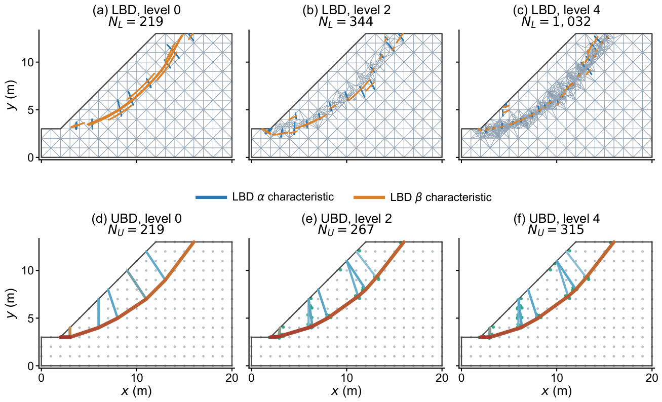
The adaptive sequence in Table 4 is monotone from both sides. The lower bound increased from to , the upper bound decreased from to , and the bracket contracted from to . The independently refined 817-point upper bound is lower because its globally uniform point cloud is substantially larger than the final 315-point adaptive cloud; it is reported as a separate reference, not as a member of the nested adaptive sequence. Figure 12 displays levels 0, 2, and 4 of the paired sequence. The upper row overlays the blue and orange lower-bound characteristic families on the adapted T3 meshes. In the lower row, the upper-bound point cloud is overlaid by the active DLO slip lines, whose colour and width increase with the normalized plastic multiplier. Thus, the panels show how each independently adapted discretization and its associated critical pattern evolve together. In this and the subsequent adaptive table, is the number of lower-bound mesh nodes and is the number of upper-bound point-cloud points.
Figure 10.
Lower-bound characteristic lines (top) and upper-bound active DLO lines (bottom) for three friction angles.
Figure 10.
Lower-bound characteristic lines (top) and upper-bound active DLO lines (bottom) for three friction angles.
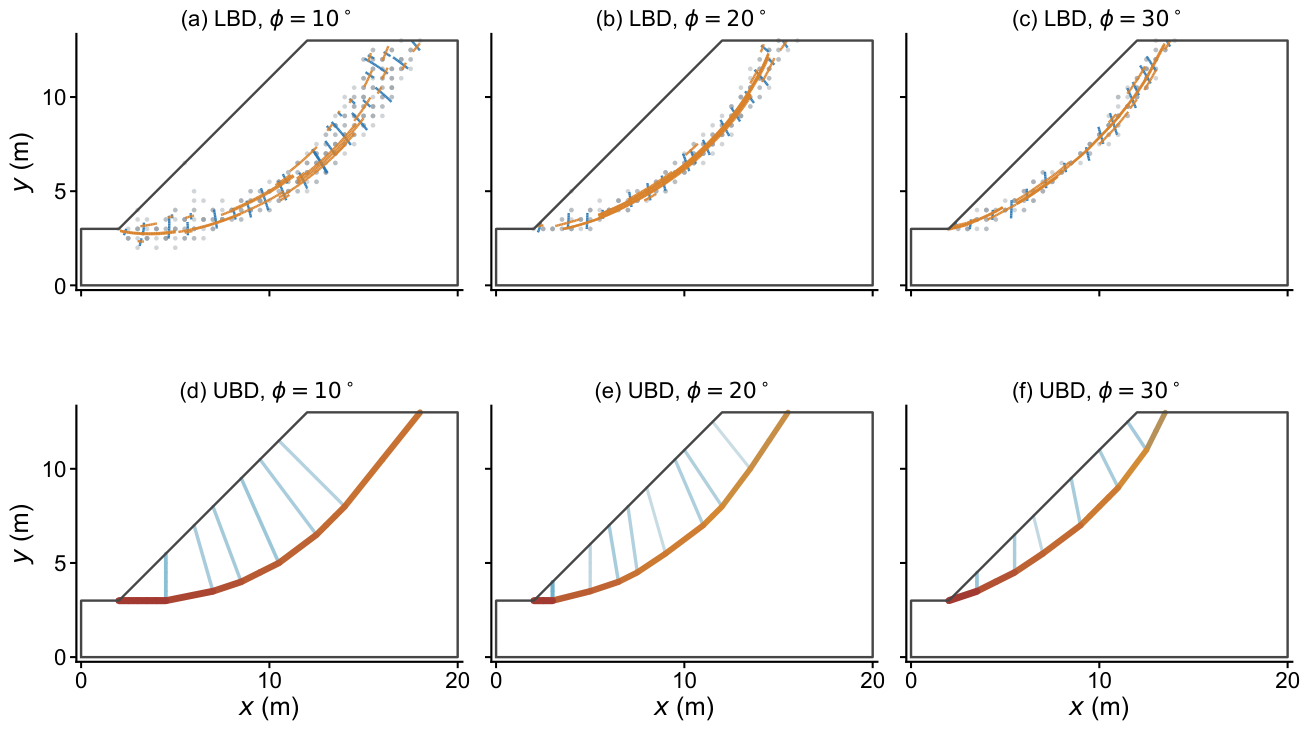
Figure 11.
Opposite monotone adaptive bound sequences for the slope.
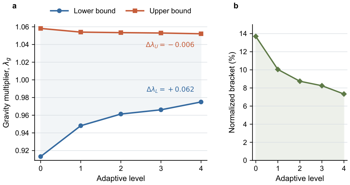
Figure 12.
Evolution of the lower-bound T3 mesh with both characteristic families and the upper-bound DLO point cloud with active slip lines.
Figure 12.
Evolution of the lower-bound T3 mesh with both characteristic families and the upper-bound DLO point cloud with active slip lines.
For the lower-bound comparison, the P1 sequence was retained through level 4, whereas the combined P2 sequence was evaluated through level 3. Each sequence used its own yield-dual indicator and therefore generated a different nested mesh family. Table 5 reports the measured optimizer cost together with the bound evolution.
At nearly equal element counts on levels 2 and 3, P2 raised the lower bound by and , respectively, but required substantially longer optimizer times. The comparison changes when a target bound is considered: the 635-element P2 solution reached in s, exceeding the 2001-element P1 value of obtained in s. P2 costs more per element but is cheaper at this target accuracy.
Figure 14 pairs the P1 h-adaptive meshes with their lexicographically selected RGB stress fields at levels 0, 2, and 4. The primary weighted jump measure decreased by , , and , respectively, while the load multiplier and maximum yield ratio were unchanged. The selected fields retain the curved toe-to-crest stress transfer as the lower bound increases. RGB values are evaluated directly from the element-local P1 interpolation under common limits, without nodal averaging or image-space smoothing. P1 is used for the selected-field panels; P2 is retained only for the bound-and-cost comparison in Table 5 and Figure 13.
4.3. Frictionless Plane-Strain Extrusion
The third benchmark is Alexander’s complete slip-line solution for frictionless plane-strain extrusion [32]. The lower half of the symmetric domain has upstream and downstream heights of 3 and 1, respectively, giving a 3:1 reduction. The die corner is at , and both straight channel extensions have length 6. The material is weightless and rigid-perfectly plastic. Tresca yielding is recovered from Mohr–Coulomb plasticity by setting and . The inlet ram, symmetry line, and die walls are tangentially smooth, the outlet is traction free, and the objective is the mean compressive inlet pressure p. Alexander’s exact value is
Figure 15 summarizes the half-domain geometry and the boundary conditions shared by both bound calculations. The inlet segments carry the unknown normal reaction in the lower-bound problem and share one normal velocity in the upper-bound problem.
Both bounds started from the same 40-point geometry. The initial lower-bound mesh contained 48 checker-pattern T3 elements, whereas the initial upper-bound network contained 397 admissible lines. Twelve independent adaptive updates were completed. The upper-bound cloud accepted at most 20 new points per update. On the lower-bound side, repeated all-edge refinement was found to spend most new elements within the already localized die region. For this example, at most 80 elements were therefore marked per update and were refined by conforming longest-edge bisection. This calculation control changes neither the yield-dual indicator nor the static admissibility constraints, and the resulting meshes remain nested.
Table 6 lists alternate common states to keep the two sequences on the same update coordinate. The complete 13-state histories are plotted in Figure 16(a). The lower bound increased from 2.982165 to 3.385592, while the upper bound decreased from 3.833333 to 3.511024. At update 12, the two values lie below and above Eq. (37), respectively. The normalized bracket decreased from to . Figure 16(b) reports cumulative core time after one unrecorded warm-up solve. LBD time contains the primary lower-bound optimization, while UBD time contains both candidate-line generation and upper-bound optimization. The optional fixed-bound stress-selection solves used only for visualization are excluded.
Figure 17 shows four of the common states. The top row superposes the blue and orange characteristic families on the lower-bound meshes. Refinement remains concentrated near the die entry, while both channel far fields remain coarse. The middle row shows the independently adapted upper-bound points and active DLO lines in the same region. The bottom row gives the lexicographically selected RGB stress fields at the same lower-bound values. The selection reduced the weighted tangential-jump measure from 44.43 to 11.51, 39.46 to 10.17, 58.57 to 22.57, and 67.41 to 13.49 at updates 0, 4, 8, and 12, respectively, without changing or the maximum yield ratio. Thus, the bottom row is another optimum within the fixed-bound admissible set rather than a smoothed image. The lower-bound rows provide static information; the upper-bound row remains a kinematically admissible collapse mechanism.
5. Discussion
The lower-bound guarantee in DLO-LB follows from the stress discretization rather than the candidate-line network. A complete-line inequality controls only an integrated resultant and can admit local over-yielding, as the line-only Prandtl calculation shows. Reversing the DLO objective or replacing velocity jumps with line forces is therefore insufficient, consistent with earlier pseudo lower-bound formulations [26]. In DLO-LB, T3 equilibrium, prescribed and continuous tractions, and pointwise polygonal yield constraints are imposed on the stress field. The intersecting DLO lines serve stress projection and visualization.
DLO-LB and DLO-UB are independent workflows sharing geometry, material, loading, and boundary inputs. DLO-UB returns a kinematically admissible collapse mechanism, whereas DLO-LB returns a conservative capacity and an equilibrated, yield-admissible stress field. Yield-constraint duals trace the Mohr–Coulomb characteristic families and guide lower-bound refinement. The selection in Section 2.6.1 chooses a reproducible member of the possibly non-unique optimal stress set without changing the load multiplier. Similar critical regions support a common failure interpretation, but static characteristics are neither a velocity mechanism nor a constitutive loading path. VDLO instead projects an externally supplied instantaneous stress field onto candidate lines; the external analysis provides any load or time evolution.
Verification is currently limited to homogeneous, plane, associated perfect plasticity with T3 stress spaces. Q4 results remain supplementary because Gauss-point collocation does not ensure element-wide equilibrium, while large candidate-line sets may dominate the cost. Extensions should address equilibrated quadrilateral spaces, scalable line generation, heterogeneous or non-associated materials, three-dimensional equilibrium, finite deformation, and softening. Within this scope, the paired solutions provide conservative capacity, an explicit collapse mechanism, and a numerical bracket.
6. Conclusions
A lower-bound DLO formulation was derived for plane perfect plasticity. Its lower-bound status follows from element-local nodal stresses, exact T3 equilibrium, traction continuity, prescribed stress boundaries, and pointwise inward Mohr–Coulomb constraints. The intersecting DLO lines remain available for stress projection, but complete-line strength constraints alone do not guarantee a lower bound.
The Prandtl, slope, and plane-strain extrusion calculations produced increasing lower bounds and decreasing upper bounds under separate adaptive refinements. The extrusion sequence bracketed the exact slip-line pressure. The associated static characteristics and upper-bound mechanisms occupied similar critical regions, although they remain mechanically different fields. These results are limited to T3 stress spaces and homogeneous, plane, associated perfect plasticity. Equilibrated quadrilateral spaces, scalable line generation, and heterogeneous or non-associated materials remain open.
Acknowledgments
The authors gratefully acknowledge the financial support from the Primary Research and Development Plan of Zhejiang Province, China (Grant No. 2025C02046), the Science Foundation of Zhejiang Sci-Tech University, China (Grant No. 25052015-Y) and the Key Research and Development Plan of Hangzhou, China (Grant No. 2025SZD1A43).
References
- Chen, Wai-Fah. Limit Analysis and Soil Plasticity; Elsevier: Amsterdam, 1975. [Google Scholar]
- Lysmer, John. Limit analysis of plane problems in soil mechanics. J. Soil Mech. Found. Div. ASCE 1970, 96(4), 1311–1334. [Google Scholar] [CrossRef]
- Sloan, Scott W. Lower bound limit analysis using finite elements and linear programming. Int. J. Numer. Anal. Methods Geomech. 1988, 12(1), 61–77. [Google Scholar] [CrossRef]
- Krabbenhøft, Kristian; Damkilde, Lars. A general non-linear optimization algorithm for lower bound limit analysis. Int. J. Numer. Methods Eng. 2003, 56(2), 165–184. [Google Scholar]
- Lyamin, Andrei V.; Sloan, Scott W. Lower bound limit analysis using nonlinear programming. Int. J. Numer. Methods Eng. 2002, 55, 573–611. [Google Scholar] [CrossRef]
- Lyamin, Andrei V.; Sloan, Scott W.; Krabbenhøft, Kristian; Hjiaj, Mohammed. Lower bound limit analysis with adaptive remeshing. Int. J. Numer. Methods Eng. 2005, 63(14), 1961–1974. [Google Scholar] [CrossRef]
- Smith, Colin C.; Gilbert, Matthew. Application of discontinuity layout optimization to plane plasticity problems. Proc. R. Soc. A Math. Phys. Eng. Sci. 2007, 463(2086), 2461–2484. [Google Scholar] [CrossRef]
- Zhang, Yiming; Wang, Xueya; Wang, Xinquan; Mang, Herbert A. Virtual displacement based discontinuity layout optimization. Int. J. Numer. Methods Eng. 2022, 123(22), 5682–5694. [Google Scholar] [CrossRef]
- Gilbert, Matthew; Smith, Colin C.; Haslam, I. W.; Pritchard, T. J. Application of discontinuity layout optimization to geotechnical limit analysis problems. In Numerical Methods in Geotechnical Engineering: Proceedings of the 7th European Conference on Numerical Methods in Geotechnical Engineering, Trondheim, Norway, 2010; CRC Press; pp. pages 169–174. [Google Scholar] [CrossRef]
- Smith, Colin C.; Gilbert, Matthew. Identification of rotational failure mechanisms in cohesive media using discontinuity layout optimisation. Géotechnique 2013, 63(14), 1194–1208. [Google Scholar] [CrossRef]
- Hawksbee, Samuel; Smith, Colin C.; Gilbert, Matthew. Application of discontinuity layout optimization to three-dimensional plasticity problems. Proc. R. Soc. A Math. Phys. Eng. Sci. 2013, 469(2155), 20130009. [Google Scholar] [CrossRef]
- Smith, Colin C.; Gilbert, Matthew; He, Linwei; González-Castejón, Juan; Ouakka, Soufiane. Recent advances in the application of discontinuity layout optimization to geotechnical analysis and design problems. In Proceedings of the XVII European Conference on Soil Mechanics and Geotechnical Engineering, 2019. [Google Scholar] [CrossRef]
- Gilbert, Matthew; He, Linwei; Smith, Colin C.; Le, Canh V. Automatic yield-line analysis of slabs using discontinuity layout optimization. Proc. R. Soc. A Math. Phys. Eng. Sci. 2014, 470(2168), 20140071. [Google Scholar] [CrossRef] [PubMed]
- He, Linwei; Gilbert, Matthew. Automatic rationalization of yield-line patterns identified using discontinuity layout optimization. Int. J. Solids Struct. 2016, 84, 27–39. [Google Scholar] [CrossRef]
- He, Linwei; Gilbert, Matthew; Shepherd, Marcus. Automatic yield-line analysis of practical slab configurations via discontinuity layout optimization. J. Struct. Eng. 2017, 143(7). [Google Scholar] [CrossRef]
- He, Linwei; Schiantella, Mattia; Gilbert, Matthew; Smith, Colin C. A python script for discontinuity layout optimization. Struct. Multidiscip. Optim. 2023, 66, 152. [Google Scholar] [CrossRef]
- Grillanda, Nicola; He, Linwei; Gilbert, Matthew; Smith, Colin C. Automatic yield-line analysis of out-of-plane loaded masonry cladding panels. Comput. Struct. 2024, 305, 107563. [Google Scholar] [CrossRef]
- Schiantella, Mattia; Gilbert, Matthew; Smith, Colin C.; He, Linwei; Cluni, Federico. Limit analysis of 2d non-periodic masonry walls via discontinuity layout optimization. Int. J. Archit. Herit. 2025, 19(10), 2422–2442. [Google Scholar] [CrossRef]
- Valentino, John; He, Linwei; Gilbert, Matthew. Application of discontinuity layout optimization to metal shells and assemblies. Int. J. Numer. Methods Eng. 2026, 127(5), e70287. [Google Scholar] [CrossRef]
- Zhang, Yiming. Multi-slicing strategy for the three-dimensional discontinuity layout optimization (3d dlo). Int. J. Numer. Anal. Methods Geomech. 2017, 41(4), 488–507. [Google Scholar] [CrossRef] [PubMed]
- Zhang, Yiming; Zhuang, Xiaoying. Defining a “shallow” tunnel by stability analysis with discontinuity layout optimization. Proceedings of GeoShanghai 2018 International Conference: Tunnelling and Underground Construction, 2018a; Springer Singapore; pp. pages 131–135. [Google Scholar] [CrossRef]
- Zhang, Yiming; Zhuang, Xiaoying; Lackner, Roman. Stability analysis of shotcrete supported crown of NATM tunnels with discontinuity layout optimization. Int. J. Numer. Anal. Methods Geomech. 2018, 42(11), 1199–1216. [Google Scholar] [CrossRef]
- Sun, Zizheng; Zhang, Yiming; Yuan, Yong; Mang, Herbert A. Stability analysis of a fire-loaded shallow tunnel by means of a thermo-hydro-chemo-mechanical model and discontinuity layout optimization. Int. J. Numer. Anal. Methods Geomech. 2019, 43(16), 2551–2564. [Google Scholar] [CrossRef]
- Yan, Xiao; Sun, Zizheng; Li, Shucai; Liu, Rentai; Zhang, Qingsong; Zhang, Yiming. Quantitatively assessing the pre-grouting effect on the stability of tunnels excavated in fault zones with discontinuity layout optimization: A case study. Front. Struct. Civ. Eng. 2019, 13(6), 1393–1404. [Google Scholar] [CrossRef]
- Wang, Xueya; Zhang, Yiming; Sun, Zizheng; Ke, Fuyang. Stability analysis of tailings dam based on adaptive discontinuity layout optimization. J. Shandong Univ. (Engineering Science) In Chinese. 2023, 53(1), 100–105. [Google Scholar] [CrossRef]
- Hawksbee, Samuel John. 3D Ultimate Limit State Analysis Using Discontinuity Layout Optimization. PhD thesis, University of Sheffield, 2012. [Google Scholar]
- Smith, Colin C.; Gilbert, Matthew. The stress function basis of the upper bound theorem of plasticity. Int. J. Solids Struct. 2022, 244–245, 111565. [Google Scholar] [CrossRef]
- Zhang, Yiming; Zhuang, Xiaoying. Cracking elements: A self-propagating strong discontinuity embedded approach for quasi-brittle fracture. Finite Elem. Anal. Des. 2018b, 144, 84–100. [Google Scholar] [CrossRef]
- Zhang, Yiming; Mang, Herbert A. Global cracking elements: A novel tool for Galerkin-based approaches simulating quasi-brittle fracture. Int. J. Numer. Methods Eng. 2020, 121(11), 2462–2480. [Google Scholar] [CrossRef]
- Mu, Linlong; Zhang, Yiming. Cracking elements method with 6-node triangular element. Finite Elem. Anal. Des. 2020, 177, 103421. [Google Scholar] [CrossRef]
- Wang, Xueya; Zhang, Yiming. Stability analysis with discontinuity layout optimization: strength reduction vs gravity increasing. Hazard Control Tunn. Undergr. Eng. In Chinese. 2021, 3(3), 94–99. [Google Scholar]
- Alexander, J. M. On complete solutions for frictionless extrusion in plane strain. Q. Appl. Math. 1961, 19(1), 31–37. [Google Scholar] [CrossRef]
Figure 1.
Schematic construction of DLO-LB on a half-Prandtl domain: (a) Sloan-type stress mesh; (b) intersecting DLO topology; (c) VDLO stress-to-line projection and line-level Mohr–Coulomb constraint; and (d) an illustrative critical line pattern.
Figure 1.
Schematic construction of DLO-LB on a half-Prandtl domain: (a) Sloan-type stress mesh; (b) intersecting DLO topology; (c) VDLO stress-to-line projection and line-level Mohr–Coulomb constraint; and (d) an illustrative critical line pattern.
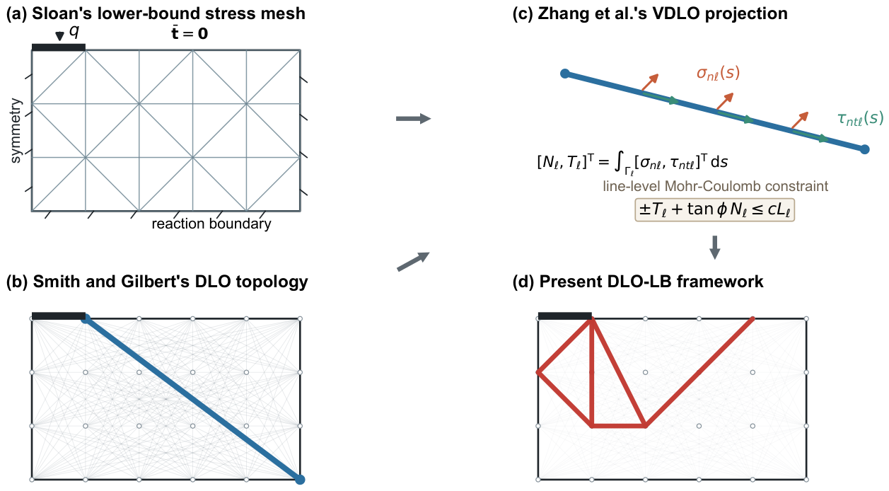
Figure 3.
Complete Prandtl model and the coarsest lower- and upper-bound discretizations.

Figure 4.
Complete-domain Prandtl bounds and normalized bracket under refinement.
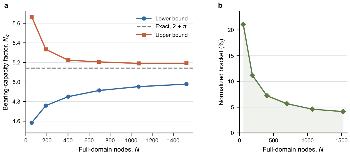
Figure 5.
Complete symmetric Prandtl punch: traced lower-bound characteristics and independent upper-bound mechanisms on coarse and fine grids.
Figure 5.
Complete symmetric Prandtl punch: traced lower-bound characteristics and independent upper-bound mechanisms on coarse and fine grids.
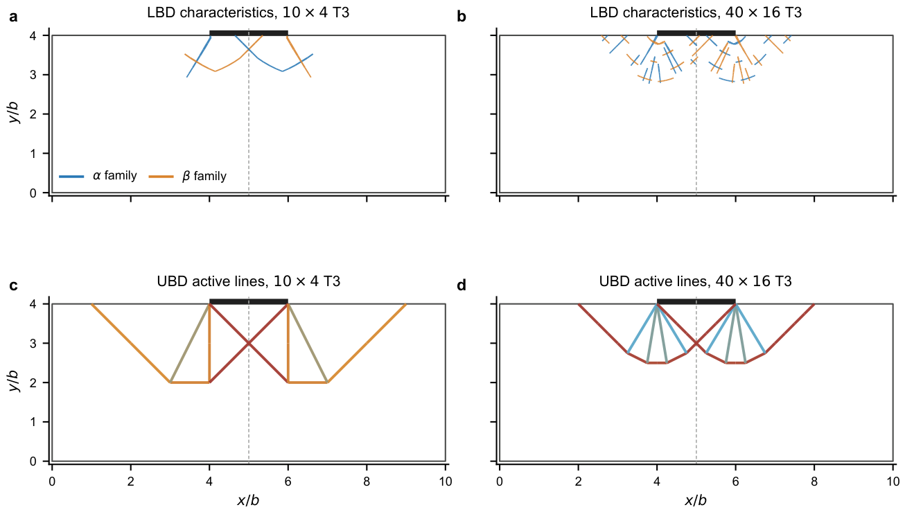
Figure 6.
Prandtl stress fields before and after lexicographic selection at the same lower bound.
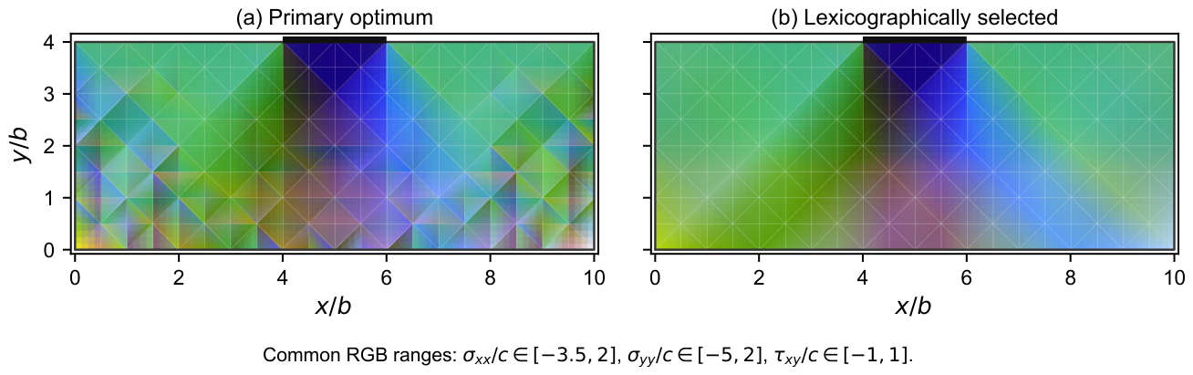
Figure 7.
Mirror-paired Prandtl meshes for P1 h and P2 adaptivity.
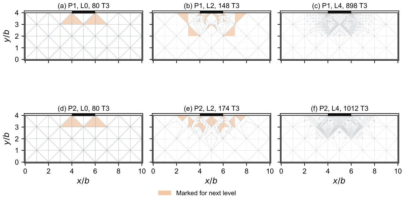
Figure 8.
Prandtl lower-bound evolution and optimizer cost for mirror-paired P1 h and P2 combined adaptivity.
Figure 8.
Prandtl lower-bound evolution and optimizer cost for mirror-paired P1 h and P2 combined adaptivity.
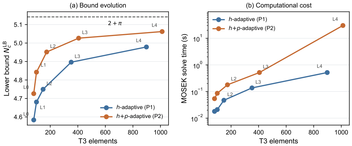
Figure 9.
Lower and upper gravity multipliers for the same slope as varies.
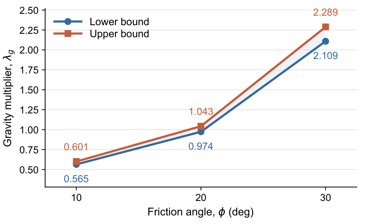
Figure 13.
Slope lower-bound evolution and optimizer cost for P1 h versus P2 .
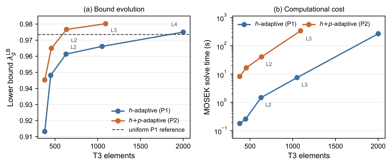
Figure 14.
P1 h-adaptive meshes and selected stress fields for the slope.
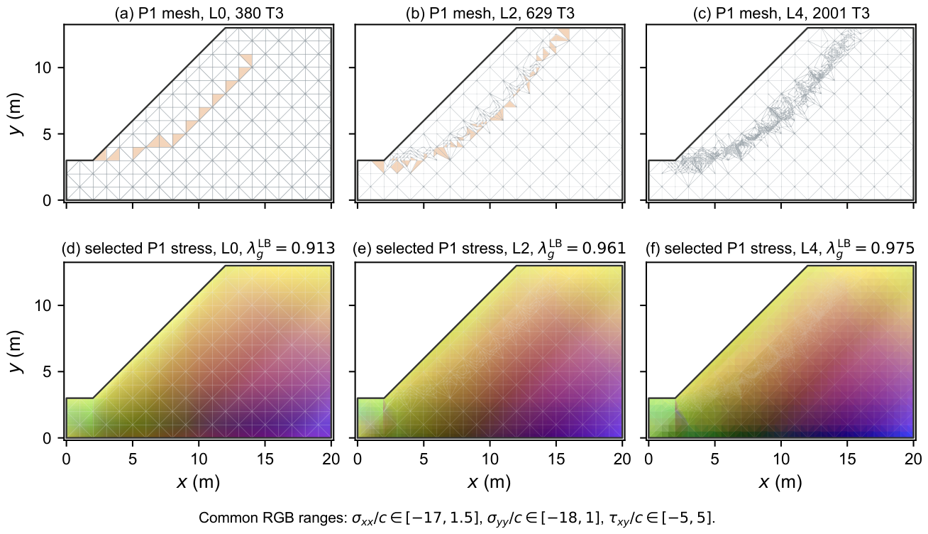
Figure 15.
Half-domain geometry and boundary conditions for the frictionless 3:1 Alexander extrusion problem.
Figure 15.
Half-domain geometry and boundary conditions for the frictionless 3:1 Alexander extrusion problem.
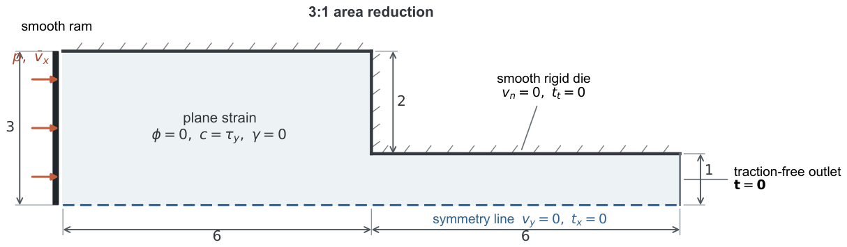
Figure 16.
Adaptive Alexander extrusion bounds and cumulative core time.
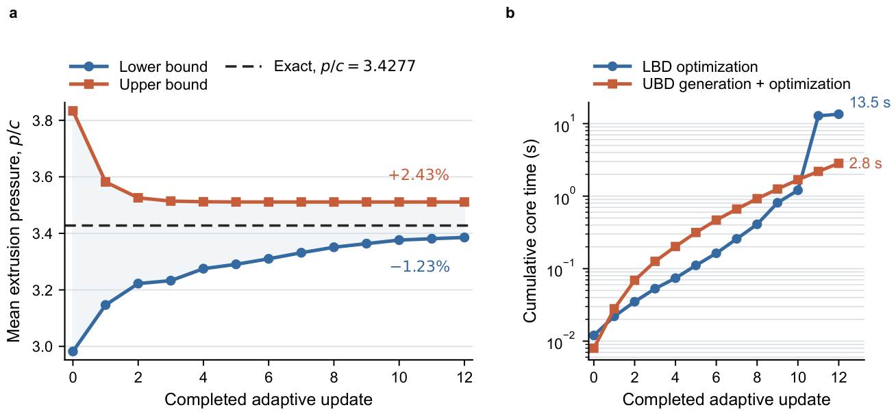
Figure 17.
Selected lower-bound characteristics and stress fields with upper-bound layouts.
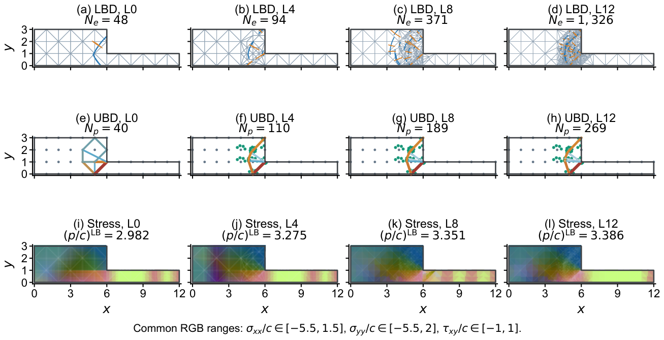
Table 1.
Complete-domain Prandtl bounds under mesh refinement.
| Half grid | Full grid | Nodes | Bracket (%) | ||
|---|---|---|---|---|---|
| 55 | 4.583742 | 5.666667 | 21.062 | ||
| 189 | 4.758506 | 5.333333 | 11.180 | ||
| 403 | 4.850373 | 5.222222 | 7.232 | ||
| 697 | 4.913473 | 5.205128 | 5.672 | ||
| 1071 | 4.952569 | 5.189610 | 4.610 | ||
| 1525 | 4.978068 | 5.190744 | 4.136 |
Table 3.
Effect of friction angle on the gravity multiplier for one slope.
| Gap (%) | |||
|---|---|---|---|
| 0.564611 | 0.600561 | 5.986 | |
| 0.973507 | 1.043328 | 6.692 | |
| 2.108661 | 2.288686 | 7.866 |
Table 4.
Paired adaptive bounds for the slope at .
| Level | T3 | Lines | Gap (%) | ||||
|---|---|---|---|---|---|---|---|
| 0 | 219 | 380 | 0.913233 | 219 | 14,506 | 1.058189 | 13.70 |
| 1 | 254 | 449 | 0.948128 | 243 | 19,975 | 1.054035 | 10.05 |
| 2 | 344 | 629 | 0.961337 | 267 | 25,864 | 1.053458 | 8.74 |
| 3 | 556 | 1051 | 0.966138 | 291 | 32,457 | 1.053026 | 8.25 |
| 4 | 1032 | 2001 | 0.974991 | 315 | 39,644 | 1.052160 | 7.33 |
Table 5.
Slope P1 h-adaptive and P2 -adaptive sequences at .
| P1 h-adaptive | P2 -adaptive | |||||
|---|---|---|---|---|---|---|
| Level | T3 | Time (s) | T3 | Time (s) | ||
| 0 | 380 | 0.913233 | 0.179 | 380 | 0.945292 | 8.237 |
| 1 | 449 | 0.948128 | 0.257 | 457 | 0.964938 | 16.657 |
| 2 | 629 | 0.961337 | 1.469 | 635 | 0.976682 | 40.474 |
| 3 | 1051 | 0.966138 | 7.482 | 1092 | 0.980232 | 336.945 |
| 4 | 2001 | 0.974991 | 266.639 | – | – | – |
Table 6.
Selected common updates for the Alexander extrusion bounds.
| Update | T3 | Lines | Gap (%) | ||||
|---|---|---|---|---|---|---|---|
| 0 | 40 | 48 | 2.982165 | 40 | 397 | 3.833333 | 22.204 |
| 2 | 48 | 64 | 3.222431 | 80 | 2,438 | 3.525868 | 8.606 |
| 4 | 64 | 94 | 3.275121 | 110 | 4,982 | 3.511904 | 6.742 |
| 6 | 104 | 170 | 3.310086 | 149 | 9,622 | 3.511084 | 5.725 |
| 8 | 207 | 371 | 3.350938 | 189 | 15,957 | 3.511028 | 4.560 |
| 10 | 446 | 841 | 3.376300 | 229 | 23,892 | 3.511024 | 3.837 |
| 12 | 691 | 1,326 | 3.385592 | 269 | 33,454 | 3.511024 | 3.572 |
Disclaimer/Publisher’s Note: The statements, opinions and data contained in all publications are solely those of the individual author(s) and contributor(s) and not of MDPI and/or the editor(s). MDPI and/or the editor(s) disclaim responsibility for any injury to people or property resulting from any ideas, methods, instructions or products referred to in the content. |
© 2026 by the authors. Licensee MDPI, Basel, Switzerland. This article is an open access article distributed under the terms and conditions of the Creative Commons Attribution (CC BY) license.
Copyright: This open access article is published under a Creative Commons CC BY 4.0 license, which permit the free download, distribution, and reuse, provided that the author and preprint are cited in any reuse.


