

Submitted:
31 July 2026
Posted:
03 August 2026
You are already at the latest version
Abstract
Extreme precipitation and hail events over complex terrain are strongly dependent by the multiscale evolution of convective systems, yet their development remains challenging to observe and model. In this study, we apply a self-supervised learning (SSL) framework to Meteosat infrared 10.8 μm imagery over the Alpine region to derive physically meaningful representations of convective cloud organization across the full daily cycle. The learned representation organizes convective cloud scenes into three primary regimes: early convection (EC), deep convection (DC), and overcasted anvil systems (OA), each exhibiting distinct cloud-top properties, spatial structures, and temporal variability consistent with established convective development stages. Extreme precipitation and hail events preferentially occur within these regimes, occupying the upper tail of cloud-top height, optical thickness, and cloud coverage distributions within the latent space, rather than forming separate clusters. This indicates that extremes correspond to rare, intense realizations of continuous convective variability. Two dominant storm evolution pathways are identified: a rapid EC→DC transition and a persistent DC mode. The former is characterized by fast cloud growth and intensification, while the latter corresponds to long-lived, mature convective systems with sustained cloud properties. Overall, the results demonstrate that infrared-based SSL representations capture physically consistent convective stages and their transitions, providing a novel observational framework for characterizing extreme convective events and supporting the evaluation of convection-resolving numerical prediction models.
Keywords:
self-supervised learning
; infrared satellite imagery
; cloud classification
; deep moist convection
; convective cloud regimes
; cloud transitions
; extreme precipitation
; severe hail
; Alps
1. Introduction
The Alps are a hotspot for heavy rainfall [1,2] and hailstorms [3,4], where climate change is projected to amplify precipitation extremes and elevate the risk of severe flooding [5,6,7].
However, accurate and timely predictions of extreme precipitation in complex orographic areas are an open challenge in numerical weather prediction (NWP) models due to their poor representation of cloud systems [8,9,10].
NWP models exhibit persistent biases in representing convection initiation [11] and precipitation over the Alps [12,13,14], partly due to limitations in representing sub-kilometer-scale processes, such as turbulence and cloud microphysics. Additionally, cloud organization is generally not explicitly represented in NWP models, despite its potential influence on the intensification and evolution of convective systems [15,16]
Observations can enrich the model with critical information that can lead to the improvement of its performances. However, conducting observations is challenging over complex terrain. Ground-based observations from past field campaigns over the Alps, such as MAP [17], HyMeX [18], Swabian MOSES [19], and the recent TEAMx [20,21] have provided valuable insights into deep moist convection over orography. However, these measurements are typically limited to specific case studies, with high spatial and temporal resolution confined to relatively small domains and short periods. Weather radar observations have been widely used to study and forecast convective systems over the Alps [22,23,24,25]. However, beyond the logistical challenges of deploying weather radars over orography, beam blockage and terrain-induced artifacts may introduce uncertainties in their convective storm characterization and precipitation estimates [26,27].
Satellite observations, with their continuous global coverage, constitute a valid alternative to ground-based measurements. Active sensors (e.g., CloudSat and EarthCARE) provide vertically resolved cloud information but suffer from limited temporal sampling [28,29], while passive microwave sensors (e.g., GPM) enable rainfall [30,31,32] and hail [33,34] retrievals but at coarse spatial and temporal resolution. Conversely, geostationary satellites provide continuous passive monitoring of cloud evolution at high temporal and moderate spatial resolution, in both visible (VIS) [35] and infrared (IR) [36] wavelengths. IR-based techniques are extensively used for the detection of convective clouds and their initiation [37,38,39,40,41,42,43], the characterization of their development and organization [43,44,45,46,47,48,49], and the nowcasting of intense precipitation [50,51]. Specific features such as overshooting tops (OTs) [52,53,54] and glaciation temperature [55] further enable the identification of storm severity. Together, these capabilities demonstrate the value of IR observations for monitoring the evolution of convective systems throughout their life cycle, although overlying cirrus clouds can obscure the IR signature of underlying convection development stages [56].
To effectively exploit the large volume of available satellite data, cloud classification has emerged as a key tool to extract structured information, investigate convective processes and the different stages of cloud development. Early work such as the International Satellite Cloud Climatology Project (ISCCP) [57] established the foundation for classifying clouds based on radiative and microphysical properties. EUMETSAT Satellite Application Facilities (SAF) support nowcasting activities and climatological analyses by providing cloud products [58,59,60] and convection products [61]. Cloud classification has also been an active area of research within machine learning (ML) applications [62]. Early approaches relied on manually engineered features extracted from satellite imagery [63,64,65]. With the increasing availability of large satellite image archives, deep learning (DL) methods have become particularly advantageous, as they eliminate the need for manual feature extraction and are highly effective at learning complex spatial patterns directly from image data [66]. DL methods have been widely applied to classify clouds [67,68], detect convection initiation and OTs [69,70,71,72], nowcasting [73], and investigate the spatiotemporal patterns of convective systems [74,75]. Because the majority of satellite observations remain unlabeled, unsupervised methods, such as self-organizing maps [76], contrastive learning [77,78], and rotationally-invariant clustering [79], have been used to identify cloud regimes across different regions and sensors. Among the unsupervised learning approaches, self-supervised learning (SSL) is particularly promising because it learns robust and transferable feature representations directly from the data [80], demonstrates resilience to dataset imbalance [81], and is therefore well suited to the study of rare extreme events. In the context of cloud classification, SSL methods have already been applied to geostationary satellite imagery. Chatterjee et al. (2023) used SSL to classify cloud systems over Germany [82,83] based on high-resolution cloud optical thickness (COT) images. Similarly, SSL methods have been applied to classify marine cloud morphologies from satellite [84,85], and have also been extended to ground-based imagery [86,87].
Despite progress in SSL-based cloud classification, existing approaches have not been applied to learning convective organization from continuous geostationary IR imagery over complex terrain, where extreme precipitation is frequent and model representation remains limited. To address this gap, this study develops a cloud-regime classification framework based on SSL applied to all-day geostationary IR observations. Building on the methodology of Chatterjee et al. (2023) [82], we classify convective cloud spatial structures and analyze their evolution in relation to extreme precipitation and hail events over the Alpine region, identified from human-reported observations in the European Severe Weather Database (ESWD) [88]. We focus on cloud structures associated with precipitating convective systems over the Alps, encompassing phenomena ranging from individual convective cells (10–20 km) to organized mesoscale convective systems (100–500 km) [59,89]. We hypothesize that extreme precipitation events are associated with recurring spatial patterns (i.e., repeatedly observed cloud morphologies in geostationary IR imagery) and transition pathways that describe the typical sequence through which these patterns evolve during an event. Identifying such patterns from continuous geostationary observations may provide new insights into the organization and evolution of convection over complex terrain while also offering a benchmark for evaluating and improving NWP model representations. Accordingly, our objective is to assess whether the SSL model can extract robust and physically meaningful representations of storm evolution from IR imagery, and to identify recurring mesoscale cloud spatial patterns and their dominant transition pathways associated with extreme precipitation events over the Alps.
Specifically, this study addresses the following research questions:
- RQ1: Can convective scenes associated with extreme precipitation and hail events be identified among all IR-based cloud scenes using SSL?
- RQ2: Can the dominant transition pathways in convective cloud patterns related to extreme precipitation and hail be characterized using the SSL-based cloud regime classification?
2. Materials and Methods
2.1. Satellite Data
In this work, we use the brightness temperature (BT) at 10.8 μm of the Meteosat Second Generation Spinning Enhanced Visible and Infrared Imager (MSG-SEVIRI; [90]). MSG-SEVIRI has an adequate spatiotemporal resolution (i.e., a native spatial resolution of approximately 5 km and a temporal sampling of 15 min) on the Alpine domain (42-51.5 N, 5-16 E, Figure 1a). Moreover, it provides continuous long-term measurements, which are essential for assembling sufficiently large datasets for robust DL training, and the 10.8 μm IR channel is available both day and night, allowing the DL model to benefit from the variability of the all-day signal. The nighttime measurements allow to include nocturnal convection in the analysis that are not included in Chatterjee et al. (2023) [82]. The selected wavelength at 10.8 μm lies within the atmospheric window, where the recorded BTs are primarily determined by the thermal emission from the cloud top for optically thick clouds [57], making them a useful proxy for cloud-top height.
We preprocessed MSG-SEVIRI data before ingesting it into the DL algorithm to preserve native spatial resolution as much as possible; we applied a correction for parallax displacement since we merged satellite observations with ground-based human reports. Furthermore, the data were linearly interpolated onto a regular latitude–longitude grid with a grid spacing of 0.04°, which corresponds approximately to 4.5 km in the north-south direction and 3.3 to 2.8 km in the east-west direction. The Climate Monitoring SAF (CMSAF) cloud mask product (CLAAS-3; [91]), based on MSG-SEVIRI observations and resampled to the same spatial grid, is used to suppress unwanted contributions from surface features (e.g., snow-covered terrain or land-sea contrasts). In the Appendix A, we report the details of the methodology we used to fill small gaps of clear sky over cloudy regions, predominantly occurring in presence of low-level clouds or snow-covered areas.
The study period extends from 2013 to 2025, covering the summer months from April to September. The summer season experiences the highest convective activity [59] and minimizes the influence of snow-covered surfaces over the Alpine region, as snow is a major source of error for the cloud mask ([91]).
2.2. Datasets Preparation
2.2.1. Training Dataset
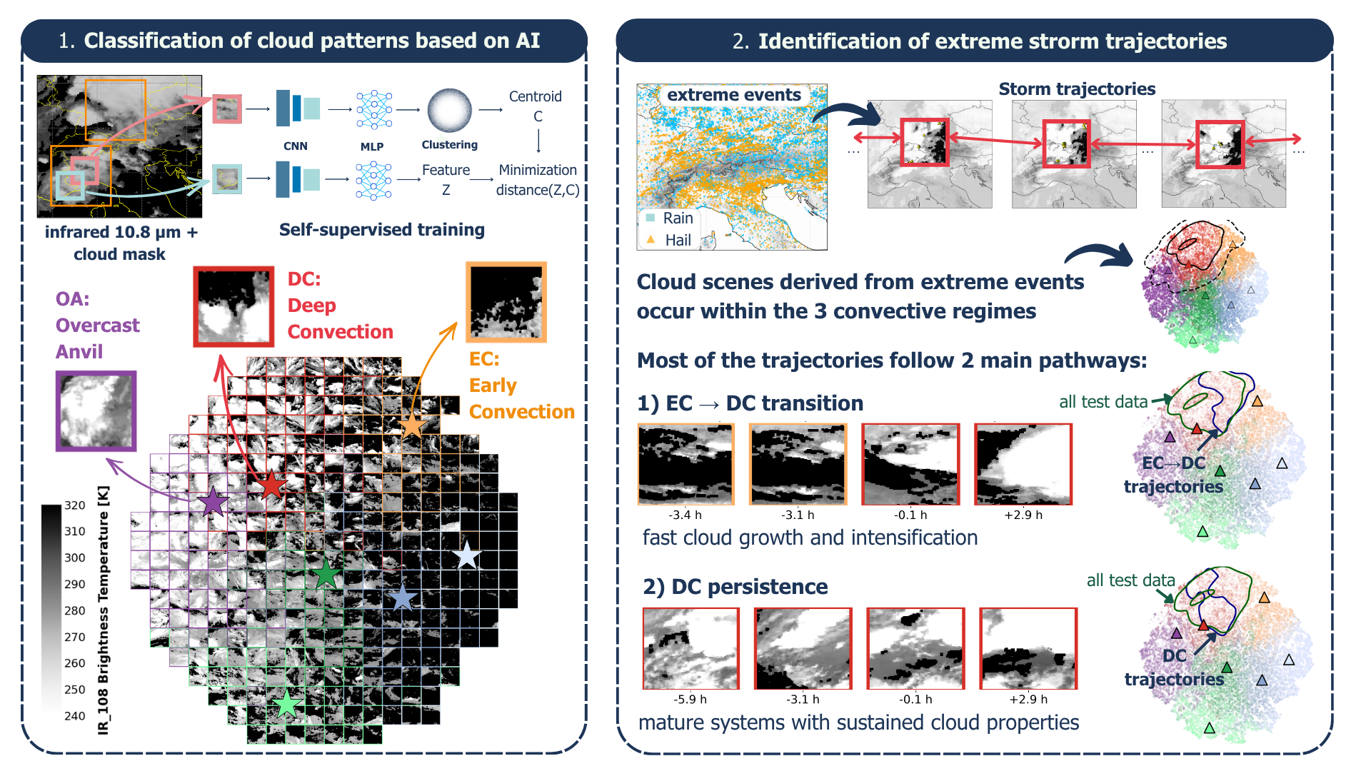
For model training, we used the years 2013, 2017, 2021, and 2025 to sample the study period as evenly as possible. The input data for training the model consist of image subsets, hereafter referred to as crops, extracted from the full Alpine domain using a fixed window size of 100 x 100 pixels. This corresponds to an approximate physical extent of 445 km in the north-south direction and km in the east-west direction, depending on latitude. The crop size encompasses the typical spatial scale of mesoscale convective systems in the region which extends from approximately 100 to 500 km [59], while remaining sufficiently compact to limit computational cost. We extract two random crops per time step to increase sample diversity and improve model generalization (Figure 1b), resulting in an average pixel overlap of less than 5% between crops. In total, we generated approximately 140,000 samples for model training. Each crop is further randomly cropped into two augmented views, which serve as the input to the SSL model (Figure 1c).
2.2.2. Test Dataset
For constructing the independent test dataset, we used the years that were not included in the training dataset, namely 2014, 2015, 2016, 2018, 2019, 2020, 2022, 2023, and 2024. The crops for the test dataset have the same size of 100 × 100 pixels but are no longer random. We selected precipitation and hail events with the highest quality control levels (QC1 and QC2, referring to confirmed reports and documented scientific case studies) from the ESWD [88] (Figure 1d). Storm trajectories were reconstructed by first clustering ESWD reports within consecutive 15-min intervals and then using a spatial clustering algorithm (Figure 1e). Then, consecutive cluster centers were linked based on spatial proximity to construct continuous storm trajectories. If no reports were available for intermediate time steps, the position of the cluster center was linearly interpolated, provided that the missing interval did not exceed four consecutive 15-min time steps (i.e., 1 hour). Moreover, trajectories were temporally extended by hours to capture the broader evolution of convective systems. Finally, satellite crops are extracted centered on the cluster centers, obtaining approximately 26,000 samples (Figure 1f). A detailed description of the trajectory reconstruction and preprocessing steps is provided in Appendix B.
2.3. Physical Characterization
To characterize the cloud regimes identified by the SSL framework, we use several cloud properties derived from the CM SAF CLAAS-3 dataset [58], including cloud cover (CC), cloud top height (CTH), and cloud optical thickness (COT) (Table 1). In addition to median CTH (CTHMedian) and median COT (COTMedian), we introduce two metrics designed to emphasize deep convective structures: the fraction of cloudy pixels with CTH exceeding 10 km (CTH10+) and the fraction with COT greater than 30 (COT30+). These thresholds are physically motivated by the typical characteristics of deep convection in mid-latitudes. CTH above 8–10 km generally indicates strong vertical development reaching the upper troposphere, while large COT values (COT > 20–30) are associated with dense, vertically developed convective clouds containing substantial ice content [57]. The CTH10+ and COT30+ metrics therefore provide proxies for the spatial extent and severity of deep convective cores within each cloud regime.
To characterize precipitation in the test crops, we employed the satellite-based IMERG Final Run product [92], which provides rain rate estimates (mm h−1) at 30-minute intervals and 0.1° spatial resolution. Although IMERG is known to exhibit uncertainties, particularly over complex terrain [93], IMERG Final Run incorporates gauge adjustment and provides a long-term, spatially continuous precipitation record with complete coverage over the Alpine region, which cannot be achieved using ground-based observations alone. We processed IMERG half-hourly rain rate data as follow: for each crop temporally matching IMERG timestamp, IMERG field is spatially cropped to the same crop domain. Then, the cumulative half-hour precipitation (mm) is obtained by summing over the rainfall rates and dividing by a factor of 2.
2.4. Self-Supervised Deep Learning Model
The SSL model used in this study, DeepCluster v.2, is implemented using the VISSL library developed by Facebook AI Research [94]. We adopted this model because it has been successfully used by Chatterjee et al. (2023) [82] for similar purposes. The architecture is illustrated in Figure 1c and more details on the training setup can be found in Appendix C. However, in this study, we train the model on IR imagery to characterize cloud structures rather than using high-resolution COT data. All other architectural components and training hyperparameters are kept identical to those of the original implementation. The model adopts a Siamese CNN architecture to extract semantic representations (features) from IR BT imagery provided as input in crops. We will refer to the ensemble of representations of our cloud imagery dataset as the feature space. The model classifies cloud scenes into a number of clusters specified by the user based on the similarities among the features extracted from each crop. In this work, we chose to identify 7 clusters following [82] who shows that this is the optimal number for the central European domain using the same SSL architecture. The substantial overlap between our domain (Figure 1a) and the study domain of [82] and their similar synoptic conditions suggest a comparable range of cloud organizational patterns, justifying the use of the same configuration.
The SSL strategy for learning which features are similar leverages multiple views of the same input image. Specifically, each crop is randomly sampled into two overlapping sub-crops, or views. These two views are not simple translations of the same crop. Instead, each view is generated by randomly shifting the crop location in space and allowing variations in both spatial extent and aspect ratio. This strategy introduces additional geometric diversity while preserving semantic consistency between views. To ensure comparability between inputs, both views are subsequently resampled to a common size of 75 × 75 pixels. For simplicity, Figure 1b illustrates only the spatial shift between the two views. This procedure encourages the model to learn features that are invariant not only to spatial displacement but also to moderate changes in scale and aspect ratio, thus improving the robustness of the learned representations [95]. The shift invariance and scale robustness of the SSL representations, learned through the multi-view augmentation strategy, ensure that the framework remains robust to the spatial uncertainty inherent in report-based crop placement, such that crops not perfectly centered over the convective core are still meaningfully represented in the learned feature space.
The backbone network is a ResNet-50 encoder [96] coupled with a Multilayer Perceptron (MLP) head that projects features extracted from an input crop to a 128-dimensional feature vector (Figure 1c). The Siamese architecture is based on two branches sharing the same backbone. Working in parallel, each branch sees only one of the two sub-views of each crop. In the first branch, a spherical k-means clustering [97] groups the feature vectors into k clusters, each represented by its centroid. As both sub-views of each pair are assumed to display similar cloud regimes, the second sub-view should end up in the same cluster. Thus, in the other branch, the extracted feature vectors of the second sub-views are directly compared to the centroids obtained from the first branch, which now act as pseudo-labels. The training loss is then computed as the cross-entropy function between these second feature vectors and their assigned pseudo-labels. Backpropagation of this loss promotes feature alignment for samples within the same cluster via cosine similarity (i.e., the normalized scalar product between two feature vectors), while increasing separation between different cloud regimes and morphologies.
For inference on the test dataset, the trained CNN encoder and the MLP projection head were used with frozen weights to compute feature vectors. Each test vector was then assigned to the nearest training centroid based on cosine similarity. The learned feature spaces reside in a 128-dimensional space, which requires dimensionality reduction for visualization. Following [82], we apply t-distributed stochastic neighbor feature space (t-SNE) [98], with principle component analysis (PCA) initialization and perplexity set to 50.
3. Results
3.1. Characterization of the Training Dataset
The DeepCluster2 model identifies seven distinct clusters in the latent space, hereafter referred to as cloud regimes. Because the clustering is purely data-driven, these regimes have no predefined physical meaning. Their physical interpretation is obtained by analyzing the cloud properties of the samples assigned to each regime.
We identified three main groups of regimes: low CC regimes, which include clear sky (CS) and shallow clouds (SC); mid-level cloud regimes, split into two classes, MC1 and MC2; convective cloud regimes, identified as early convection (EC), deep convection (DC), and overcast anvil (OA). The two-dimensional t-SNE projection of the learned feature space derived from the image crops provides evidence that supports the classification presented (Figure 2a); the feature space localized cloud images with an organization according to their morphology: low CC cloudy scenes are predominantly located on the right-hand side of the feature space, while overcast conditions occupy the left-hand side. In between these two regimes, a gradient in CC appears. The five closest and thus most representative crops to the centroids of each class (Figure 2b) illustrate the typical morphology of each class. Hereafter, white/gray shades correspond to lower BTs (cold, high cloud tops), while darker shades indicate higher BTs (warm surfaces or low-level clouds). Class CS is characterized by nearly uniform black scenes with very limited BT-based cloud features. Class SC exhibits sparse and fragmented dark-grey structures occupying a small fraction of the image. Classes MC1 and MC2 show increased CC, with a mixture of dark- and light-grey regions and subtle differences in their spatial fragmentation and organization. Class EC is characterized by weak and fragmented cloud features with predominantly darker-grey tones and limited spatial extent. Class DC displays large contiguous regions of very light-grey and white shades embedded within darker surroundings, resulting in strong spatial contrast across the scene. In contrast, class OA exhibits more homogeneous cloud coverage, with light-grey regions distributed more uniformly throughout the image and fewer areas of strong contrast.
The OA class is the most frequent, whereas EC and MC1 occur the least often (Figure 3a). If we look at the occurrence during daytime and nighttime (Figure 3a), EC and DC are the only classes exhibiting a preference for daytime occurrence, while the rest of the classes show more contributions from nighttime observations. When looking at the hourly-based diurnal cycle (Figure 3b), the peak occurrence of EC between 10 and 14 UTC suggests its association with the convection onset stage, acting as a precursor to the DC class, more frequent between 12 and 19 UTC. In contrast, CS and OA exhibit a more uniform diurnal distribution, and SC, MC1 and MC2 show a slightly enhanced nighttime occurrence from 17 to 8 UTC.
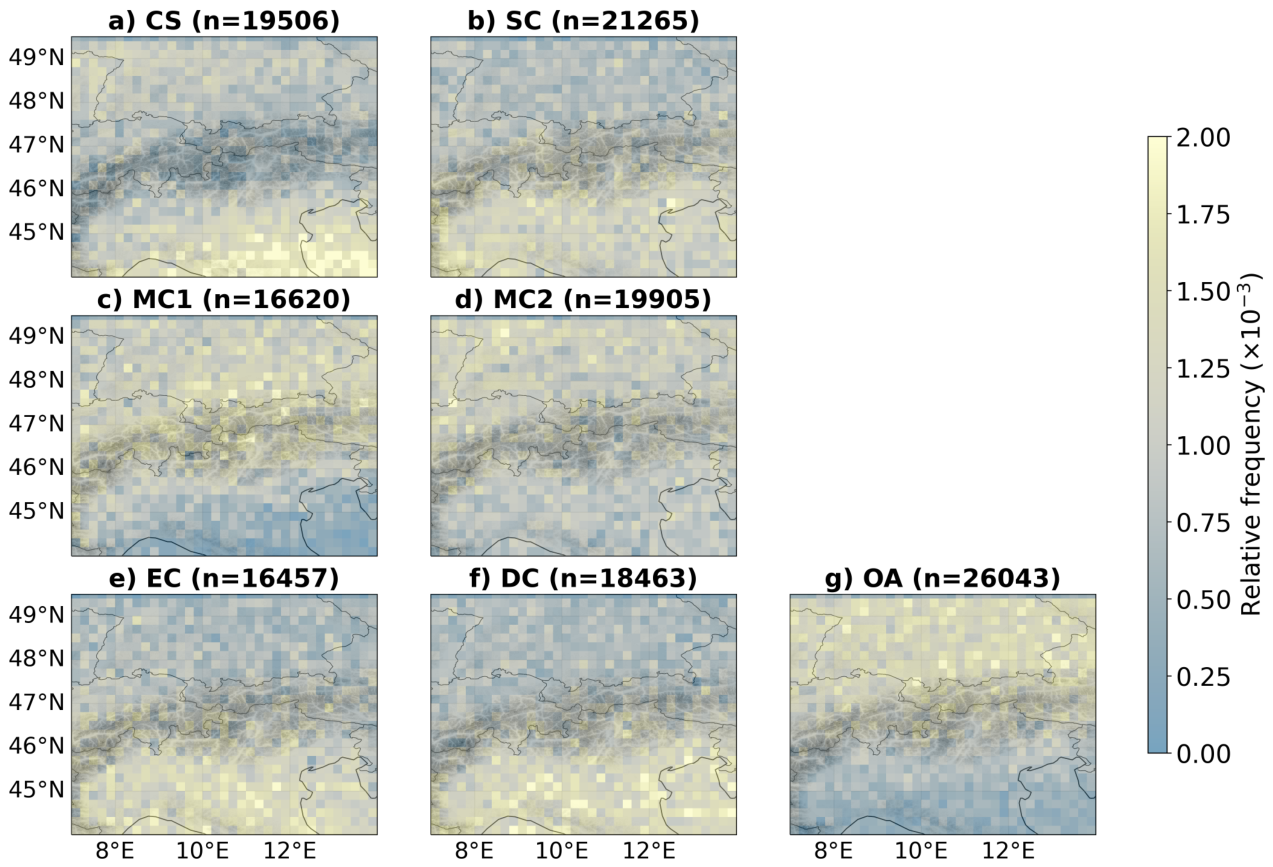
The lowest CC values of 9% and 25% occur for CS and SC, respectively (Figure 3c). Both classes show low CTHmedian values (median ) and small COTmedian (median ) (Figure 3d-e). Although CTHmedian occasionally exceeds 8 km, these cases are not associated with an increase in optical thickness (COT below ), indicating that high cloud tops mainly correspond to thin cirrus layers rather than deep convection. As shown in Figure A3a-b (Appendix D), both classes occur more frequently over the Italian part of our domain, with the strongest regional contrast observed for the CS class. The mid-level cloud regimes MC1 and MC2 are characterized by substantially higher CC than CS and SC, with MC2 exceeding 60% on average (Figure 3c). Both regimes occur preferentially during nighttime hours, suggesting an association with radiatively driven boundary-layer processes and large-scale stratiform conditions. As shown in Figure 3d-e, MC2 exhibits higher CTH (median:∼3.5 km) compared to MC1 (median:∼4 km), while MC1 shows larger COTmedian values (median ∼8 vs. ∼7). These classes are more prevalent on the northern side of the Alps, particularly for the MC1 class (Figure A3c-d). The physical distinction between MC1 and MC2 remains uncertain and may reflect either distinct stratiform regimes or different stages of cloud evolution. Disentangling these interpretations would require a more detailed analysis of regime transitions, which is beyond the scope of this study.
When looking at the convective classes, the EC class, that is morphologically similar to SC, exhibits moderate CC (mean ) much higher than SC but lower than MC1 and MC2 (Figure 3c). With a CTHmedian of about 4 km and a COTmedian of 5, this class exhibits intermediate cloud properties between SC and the mid-level classes (Figure 3d-e). Combined with its pronounced appearance between 10 and 14 UTC, this pattern suggests the development of convective cells that reach moderate heights but remain limited in horizontal extent and optical thickness, consistent with an early convective stage [48,57,59,99]. The DC class shows higher CC (median ) and larger CTHmedian values (nearly 9 km) compared to EC (Figure 3c), and COT (COTmedian generally ), larger than all other classes except OA (Figure 3d-e). This combination indicates vertically developed convective cores embedded within relatively clearer surroundings, consistent with mature convective cells [40,53,89,99]. The geographical distribution of classes EC and DC (Figure A3e-f) shows a higher occurrence in the southern Alps, a region known to be more prone to convective events [100,101]. Finally, the OA class exhibits the largest CC (Figure 3c); however, it shows lower CTH than DC (median CTHmedian around 8 km) but substantially larger COTmedian, with median around 15 (Figure 3d-e). These characteristics indicate widespread optically thick cloud shields associated with mature convective anvils. Alternatively, some cases may correspond to convective systems embedded in frontal systems characterized by very high CC (around 90%) and extensive high-level cloud layers [89,99,102]. This is further supported by the geographical distribution in Figure A3g, where this class appears more frequently on the northern side of the Alps, a region more strongly influenced by frontal systems [103].
3.2. Extreme Events Identification and Characterization
Subsequently, we investigated how the storm trajectories associated with extreme precipitation and hail in our independent test dataset evolve and are located in the learned feature space. By ingesting the test dataset into the model, we extract the associated feature vectors for each crop of the storm trajectory and investigate their characteristics. We first look at where the feature vectors of the extreme events are in the feature space (Figure 4a); the highest number of test feature vectors overlaps primarily with the convective classes EC, DC, and OA, with a minor contribution from MC2. In particular, the densest 90th percentile contoured region is centered on class DC, previously identified as mature deep convection, with only a minor superposition with EC. In the test set, nearly 60% of samples are classified as DC, while EC and OA each account for slightly less than 20%, with the remaining classes contributing only a negligible fraction (Fig. 4b). Thus, extreme events are predominantly associated with the convective regimes EC, DC, and OA.
Extreme events can be identified within the feature space, i.e. it can be assessed both visually in the t-SNE projection and quantitatively through the cosine similarity to class centroids. For EC (Fig 4c), extreme-event samples are predominantly located near the boundary with the DC class, suggesting that these cases may already exhibit characteristics of more vertically developed convection, which is consistent with the way storm trajectories were built. As expected, the distribution of the cosine similarity between EC-classified samples and their centroid (Fig 4f) shows that test samples are, on average, farther from the centroid (peak at ∼0.84) compared to the training samples (∼0.88). For DC, as reported in Fig 4d, test samples are grouped both close to the centroid and toward the outer edge of the class, away from neighboring regimes. This is reflected in the cosine similarity distribution (Fig 4g), where test samples peak at lower similarity (∼0.80) than training samples (∼0.86). For OA (Fig 4e), the feature-space distribution is more heterogeneous, with multiple high-density regions, including one near the centroid and others toward the periphery of the class. This is consistent with the cosine similarity distribution (Fig 4h), which is shifted toward lower similarity compared to the training set (peaks at ∼0.83 vs ∼0.90) and exhibits a broader shape.
Overall, extreme-event samples are not randomly distributed within the feature space but occupy specific regions, generally located farther from class centroids. This is consistent with their interpretation as tail realizations of the underlying cloud regimes, indicating that extreme events correspond to less frequent, specific realizations of each regime in the learned representation space. The OA class represents a partial exception, showing a more dispersed and irregular structure, which may reflect the inclusion in the OA class of different cloud regimes, including anvil outflow from isolated convective cells and embedded convection within frontal systems.
To assess how extreme events differ from the training distribution, we compare their physical properties across the identified three convective regimes. The 24 hours distribution (Figure 5a) shows that EC events are strongly daytime-driven, with a peak around 13 UTC, compared to a peak near 12 UTC in the training dataset. DC events occur throughout the diurnal cycle and reach a maximum near 16 UTC, whereas the training dataset exhibits a broader peak between 15 and 18 UTC. OA events are more evenly distributed in time, with only a modest late-afternoon enhancement. Relative to the training dataset, nighttime occurrences are markedly reduced in both EC and DC. Furthermore, EC events are shifted slightly toward later occurrence times. Overall, approximately 40% of events occur during nighttime (17–04 UTC), indicating a substantial contribution from nocturnal convection. This behavior agrees with previous studies of Alpine convection, reporting afternoon initiation over mountainous terrain followed by mature, organized convection and mesoscale system development later in the day [47,104,105].
In Figure 5b we observe that all test convective classes are shifted toward higher CC with respect to the training dataset. The largest shift is observed for OA where minimum CC is 30% for training and 70% for test dataset. This indicates that extreme events are generally associated with more spatially extensive cloud systems, consistent with a stronger anvil development. A clearer separation emerges in the joint distribution of and (Figure 5c–e). Across all convective classes, test samples are systematically shifted toward higher CTH and COT values than in the training set. The shift is moderate for EC (considerable shift towards higher values only for ), stronger for DC (mean increasing to 9.25 km), and most pronounced for OA, which reaches the highest optical thickness values (mean 20). These results indicate that extreme events are consistently associated with enhanced vertical development and increased optical depth, with OA showing the strongest deviation from its training distribution. This behavior becomes more evident when examining CTH10+ and COT30+ (Figure 5f–h). For EC, extreme events already exhibit a non-negligible fraction of high cloud-top and optically thick pixels (CTH10+ around 30%, COT30+ around 15%), suggesting early presence of localized intense convective cores. DC shows the most pronounced enhancement in both metrics, with mean CTH10+ and COT30+ increasing to 46% and 26%, respectively. OA exhibits a distinct regime, characterized by high COT30+ (peaking between 20–50%) but comparatively lower CTH10+, consistent with optically thick but vertically more stratified cloud shields.
Extreme precipitation and hail events do not constitute distinct cloud regimes but rather more intense realizations of common convective states. Their systematically colder, optically thicker, and more extensive cloud tops are consistent with stronger vertical development and larger anvils, characteristic of organized deep convection [89,106,107]. This suggests that the SSL representation captures cloud morphology and storm organization from IR observations alone, consistent with previous studies linking IR cloud-top patterns to the dynamical state of deep convection [39,48,49,55].
Building on this representation, we next investigate how convective systems evolve within the feature space by analyzing storm transition pathways across the identified classes, providing further insight into the dynamical organization of extreme events.
3.3. Transition Pathways Analysis
After identifying the storm trajectories, we analyze the temporal variability of cloud-class labels along each path. Trajectories are grouped according to the number of distinct convective classes (EC, DC, OA) encountered: persistent (only one class), binary (two distinct classes), and trinary (all three classes or sequences involving two transitions, e.g., two identical states separated by a different one). Further details are provided in Appendix E. In total, 338 storms follow persistence pathways, 380 binary pathways, and 156 trinary pathways. We observe 16 of the 21 possible combinations and retain only pathways occurring at least 10 times. Table 2 shows the full list of these pathways. Two pathways clearly dominate the distribution: the EC→DC transition and the persistence of DC. Although the two most frequent pathways are not associated with the highest values of the selected cloud properties, they account for most of the identified storm trajectories. Therefore, the following analysis focuses on their temporal evolution to characterize the typical evolution of severe convective storms.
To characterize the average temporal evolution of each pathway, the 15-min satellite crops within each trajectory were first aggregated into hourly bins. All trajectories were then temporally aligned by defining the midpoint of each trajectory (the time around which the reported extreme events are expected by construction) as the common reference (). Relative hourly bins were subsequently defined before and after this reference time, allowing statistics to be computed across all trajectories at equivalent stages of their evolution. To ensure robust estimates, hourly bins with fewer than 100 crops were excluded from the statistical analysis of pathway temporal evolution, after pooling all trajectories for each pathway.
Figure 6 presents representative BT image crops from one selected trajectory for each of the two pathways. The EC→DC pathway (Figure 6a) exhibits a gradual and organized expansion of the cold BT region (white), which is clearly contrasted against a predominantly dark background, indicative of clearer-sky or low-cloud surroundings. In contrast, the DC persistence pathway (Figure 6b) is characterized by an extensive cold BT area already at the initial stages with a non-regular expansion evolution, while the surrounding background appears more uniformly overcast throughout the trajectory.
3.3.1. EC → DC Transition
The pathway characterized by the EC→DC transitions is described in Figure 7.a. T-SNE-based space in Figure 7.1a shows that the trajectories following the EC→DC pathway occupy an intermediate position between EC and DC cloud regimes. The temporal evolution of the cosine similarity (Figure 7.2b) shows a clear decrease in similarity to the EC centroid, accompanied by a corresponding increase in similarity to the DC centroid. This indicates that the trajectories progressively move through the feature space from regions associated with the EC cluster toward those associated with the DC cluster, passing through the transition region between the two centroids. Most of the transitions from class EC to DC happens from to . Along the trajectories as shown in Figure 7.3a, cloud properties evolve monotonically: CTHmedian increases from 6 km to nearly 11 km, being above 10 km from on, while COTmedian shows a significant increase only of the 75th percentiles. Interestingly, the maximum slope of the CTHmedian happens during the period with highest class transitions. Consistently, CC, CTH10+, and COT30+ increase from 50%, 20%, and 0% to 75%, 60%, and 25%, respectively, reflecting progressive convective intensification (Figure 7.4a). Noticeably, CC reaches its maximum already at , while CTH10+ keeps increasing until . Cumulative rain also show an increasing trend in Figure 7.5a, going from 500 mm to a maximum of 2500 mm at . Overall, the number of trajectory crops is higher during daytime conditions. However, as the trajectories progress, the storm evolution increasingly shifts toward nighttime conditions. In particular, from , the trajectories are more likely to occur during the night (Figure 7.6a).
The EC→DC pathway, characterized by fast vertical intensification, might resembles the convective development described in previous IR-based studies [39,48,49,55], in which storms undergo rapid cloud-top cooling prior to the onset of mature deep convection. Several IR-based studies also link cloud-top cooling to severe-weather development, described by glaciation processes, updraft strength, and precipitation intensity [39,40,43,55,108].
3.3.2. DC Persistence
Figure 7.b describes the DC persistence pathway temporal trends. In the t-SNE-based space shown in Figure 7.1b, DC-persistent trajectories cluster tightly around the DC centroid. Interestingly, some trajectories are found in a secondary population toward the class periphery. Cloud property-wise, the population closer to the centroids trajectories exhibit lower cloud fraction and weaker vertical development than peripheral ones (CC: 71% vs 85%; CTHmedian: 9.2 vs 10.2 km; COTmedian: 10.2 vs 12.1). The cluster of trajectories further from the centroid is also associated with more hail reports, and the trajectory including the European record hail event of 19 cm diameter reported in Figure 6b belong to that feature space region. The cosine similarity to the DC centroid remains nearly constant at approximately 0.85 throughout the trajectory, indicating that the trajectory crops consistently occupy the vicinity of the DC cluster in feature space without converging to or diverging from the DC cluster centroid (Figure 7.2b). CTHmedian and COTmedian exhibit only modest increases, from approximately 9 to 11 km and from 5 to 20, respectively, indicating that the system is already in a mature convective state (Figure 7.3b). Nevertheless, the 75th percentile of COT reaches values exceeding 50, consistent with continued cell intensification toward the end of the trajectories. The temporal evolutions of cloud area fractions, reported in Figure 7.4b, show that CC is almost constant around 80%, indicating renewed vertical activity without substantial horizontal expansion. However, CTH10+ and COT30+ rise their area fractions from 40% and 10% to 70% and 40% . Regarding cumulative rainfall (Figure 7.5b), precipitation has already accumulated to approximately 2,000 mm at the beginning of the trajectories and increases to around 3,000 mm by their end. The 75th percentile reaches values of up to 5,000 mm, indicating that a substantial fraction of the trajectories is associated with highly precipitating systems especially towards the end of the trajectories. The trajectory crops are distributed almost equally between daytime and nighttime conditions; however, after (), they are increasingly likely to occur during nighttime (Figure 7.6b).
Persistent DC trajectories might represent long-lived, organized deep convective systems characterized by sustained cold cloud tops that frequently extend into nighttime hours, consistent with mature mesoscale convection [89,104,106,107]. Over the Alpine region, such persistence could be associated with terrain-anchored convergence zones, moist southerly inflow from the Po Valley, and continuous CAPE replenishment, all of which support sustained updrafts and prolonged convection [100,109].
4. Discussion
Extreme events are associated with systematic increases in CTH, COT, and CC, yet remain embedded within the continuous cloud-regime manifold learned from the training data. Rather than forming distinct cloud regimes, they populate the upper tail of existing convective regimes indicating that extremes correspond to rare, high-intensity realizations of continuous convective variability. The relationship between stronger convective organization and larger CC is not only observed in satellite data but is also reproduced in NWP simulations [110]. Nevertheless, convection-parameterizing NWP models tend to overestimate CC [47].
The two dominant pathways identified in this study represent two different modes of convective evolution. The EC→DC pathway resembles the rapid vertical intensification reported in previous IR studies, where cloud-top cooling precedes mature deep convection and severe weather [39,48,55]. The typical convective development represented by the EC→DC pathway has also been identified in convection-permitting climate models by [47]. In contrast, persistent DC trajectories might represent long-lived organized convective systems maintained by sustained moisture supply, instability, and orographic forcing over the Alpine region [100,104,107]. This behavior is also consistent with NWP-based studies of Alpine mesoscale convective systems [111,112,113]. Finally, the identified DC-persistent pathway includes extensive cold anvils and persistent deep convective cores, which might align with hail-favorable environmental conditions, where strong instability and vertical wind shear support long-lived deep convection [109,114,115].
Our SSL-derived classes are also consistent with previous cloud-regime classifications. Classical approaches based on joint histograms of COT and CTH recover comparable large-scale cloud structures [57,60,116,117], although they rely on manually designed feature spaces rather than learned representations. Likewise, the three convective regimes identified by [82] broadly correspond to our EC, DC, and OA classes, with the main difference being the presence of a distinct cirrus regime in their COT-based classification, which is expected given the reduced sensitivity of thermal IR observations to optically thin clouds [118]. A similar correspondence is found with the rotationally-invariant cloud regimes of [79], despite their model being trained globally on MODIS observations. Together, these comparisons suggest that the SSL latent space captures physically meaningful cloud regimes that find confirmation in others studies conducted with different methodology, satellite sensors and geographical domains.
Several limitations should be considered when interpreting these results. First, the effective SEVIRI spatial resolution over the Alpine region (∼4 km) limits the representation of small-scale storm structures. In addition, IR observations have limited sensitivity to optically thin cirrus and cloud microphysics [118], while uncertainties in the CMSAF cloud mask may affect low-level cloud detection under weak thermal contrast conditions [91]. Consequently, the identified classes should be interpreted as mesoscale thermal-organizational regimes rather than fully resolved storm structures. Methodological limitations also arise from the discrete clustering of the latent space. Because k-means favours approximately balanced cluster populations [97], individual classes may aggregate multiple physical cloud states. This is likely most relevant for the OA class, which probably includes several forms of mature and dissipating convection that cannot be distinguished reliably from IR imagery alone. Finally, the trajectory analysis depends on the timing of ESWD reports and a fixed temporal window around each event, which may not fully capture convective initiation.
Future extensions, such as multispectral satellite observations, the higher spatial resolution of Meteosat Third Generation, and cluster-free SSL appraoch that operate directly in a continuous latent space, may further improve the characterization of severe convection.
5. Conclusions
In this study, we applied a SSL framework to MSG-SEVIRI IR 10.8 μm imagery, combined with a cloud mask, to identify cloud regimes and characterize their relationship with extreme precipitation and hail over the Alpine region. By learning directly from unlabeled geostationary satellite observations, the model organizes cloud scenes according to their spatial morphology and thermal structure without requiring predefined classes. The use of IR imagery further enables continuous day-to-night analysis, an important advantage for severe convection, as approximately 40% of the storm trajectories in our dataset occur between 18:00 and 04:00 UTC.
Addressing RQ1, we show that storms associated with extreme precipitation and hail occupy preferential regions of the learned latent space rather than being randomly distributed. They project predominantly onto three convective regimes—EC, DC, OA—while exhibiting systematically colder, higher, optically thicker, and more spatially extensive cloud tops than the broader convective population within the same regimes. These results demonstrate that the SSL representation captures physically meaningful differences in convective organization directly from IR satellite imagery.
Addressing RQ2, two dominant evolution pathways emerge among the most intense events: a rapidly intensifying EC→DC pathway and a persistent DC pathway associated with long-lived mature convection. Together, these pathways provide a compact description of the temporal evolution of the majority of severe convective systems in our dataset and illustrate that the learned latent space could be used to study storm evolutions in addition to instantaneous cloud morphology.
Overall, this work demonstrates that SSL can recover physically interpretable representations of convective organization and evolution from geostationary IR satellite archives without supervision. The resulting cloud regimes and evolution pathways provide an observational benchmark for evaluating cloud representation in convection-permitting weather and climate models, complementing traditional pixel-based verification.
Author Contributions
Conceptualization, Da.Co. and C.A.; methodology, Da.Co. and C.A; software, Da.Co. and Dw.Ch.; validation, Da.Co.; formal analysis, Da.Co., and C.A.; investigation, Da. Co. and C.A.; resources, Da.Co. and C.A..; data curation, Da.Co., P.B.; writing—original draft preparation, Da.Co., P.B. and C.A.; writing—review and editing, Da.Co., C.A, E.C, P.B. and Dw.Ch.; visualization, Da.Co., P.B., C.A.; supervision, C.A. and E.C.; project administration, C.A.; funding acquisition, C.A. All authors have read and agreed to the published version of the manuscript.
Funding
Daniele Corradini’s work, as part of the EXPATS research group, was supported by the IDEA-S4S network and in close collaboration with the Deutscher Wetterdienst (DWD) (grant number 4823IDEAP5), funded by the Federal Ministry for Transport, BMV. Claudia Acquistapace’s work was supported by the 2021 “Rita Levi Montalcini” young researcher program (Code PGR217DXNP).
Institutional Review Board Statement
Not applicable
Data Availability Statement
The datasets and supporting materials required to reproduce the analysis will be deposited in Zenodo and made publicly available upon acceptance of the manuscript.
Acknowledgments
The authors thank Prof. Susanne Crewell and Prof. Martin Schultz for their valuable feedback, guidance, and scientific discussions during the PhD advisory committee meetings, which substantially contributed to the development of this work. The authors acknowledge the support of the European Weather Cloud infrastructure for providing access to computational resources, including GPU systems used for data processing and model training. The authors gratefully acknowledge EUMETSAT for providing access to Meteosat Second Generation (MSG) observations and CMSAF datasets, NASA for the Integrated Multi-satellitE Retrievals for GPM (IMERG) precipitation products, and the European Severe Storms Laboratory (ESSL) for providing access to the European Severe Weather Database (ESWD). For figure preparation and data visualization, colour maps from the scientific colour map suite by Crameri [119] were used. During the preparation of this manuscript, the authors used OpenAI ChatGPT (GPT-5 series) to improve the readability and clarity of the text, support code debugging, and assist with data-analysis workflows. The authors also used GitHub Copilot to support software development and code implementation. All outputs generated by these tools were critically reviewed, validated, and edited by the authors, who take full responsibility for the content of this publication.
Conflicts of Interest
The authors declare no conflicts of interest.
Appendix A. Cloud Mask
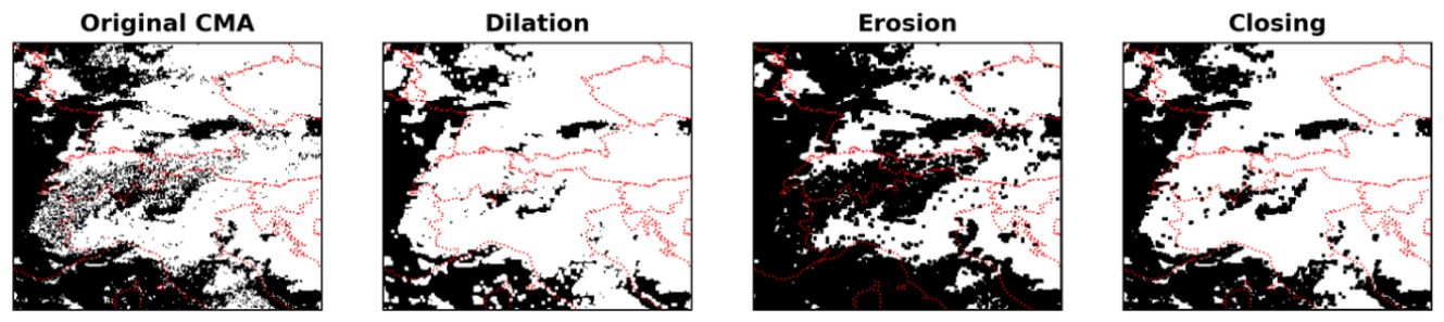
Since the IR channel lies within the atmospheric window, BT in cloud-free areas are dominated by surface signals (land, sea, ice). To focus on cloud structures, we apply a CMSAF cloud mask derived from MSG observations, retaining only cloudy pixels and assigning a baseline value of 320 K to clear-sky areas.
The CLAAS-3 cloud mask, based on a Bayesian approach trained with CALIOP observations [91], can exhibit small-scale noise (e.g., isolated clear-sky pixels within cloudy regions), especially over cold surfaces and at night. This granularity, affecting about 65% of the dataset, may bias DL models if not treated.
To reduce this noise, we apply a morphological closing (dilation followed by erosion, see Figure A1), a standard image-processing technique to remove salt-and-pepper artifacts. The optimal structuring element size was determined by comparison with the higher-resolution MODIS cloud mask (1 km). A () structuring element provided the best trade-off between noise reduction and feature preservation.
Figure A1.
Application of the closing algorithm to the cloud mask, where black represents clear sky and white represents cloud, obtained through the combination of dilation and erosion operations in image processing.
Figure A1.
Application of the closing algorithm to the cloud mask, where black represents clear sky and white represents cloud, obtained through the combination of dilation and erosion operations in image processing.
Appendix B. Storm Trajectory Reconstruction
To reconstruct the temporal evolution of convective systems, we first aggregated individual reports into 15-min time slots, matching the satellite observations’ temporal resolution. Within each time slot, ESWD reports were spatially clustered using DBSCAN [120] applied to their geographic coordinates (latitude–longitude), with a 150 km radius consistent with the 100 × 100 pixel satellite crop extent. This grouped reports associated with the same convective system, allowing satellite crops to be linked to spatially separated extreme precipitation events. The clustering procedure produced a set of cluster centroids, defined as the spatial centroids of all ESWD reports within a given 15-min time interval that belong to the same cluster. To identify transition pathways, i.e., the typical sequence of recurring cloud patterns associated with extreme precipitation events, we constructed storm trajectories based on these cluster centroids. Trajectories were obtained by linking centroids across consecutive time steps, following an approach conceptually similar to established cloud-tracking methods [121]. For each centroid, potential predecessors were searched up to 60 min backward in time at 15-min intervals. When multiple centroids were identified during the search for potential predecessors, the geographically closest centroid was selected. A cluster was assigned to an existing trajectory if the spatial displacement from the last known position was less than 200 km, and a propagation speed below ∼150 km h−1, which is consistent with observed propagation velocities of organized convective systems over Europe [59]; otherwise, a new trajectory was initiated. Trajectories with a total observed duration shorter than 30 min were discarded, as they contain too few timesteps to support meaningful pathway analysis and are likely associated with short-lived or poorly sampled events. Storm trajectories were built by linking consecutive cluster centroids up to 1 hour apart, and missing 15-minute steps were filled using linear interpolation in the latitude and longitude of the available cluster centroids positions to obtain temporally continuous tracks. To account for reporting delays and gaps inherent to human-submitted observations, we extended the trajectories by ±2 h beyond its observed temporal limits, capturing the convective organization around the reported impact and providing additional timesteps for the transition pathway analysis. The extension was performed by linearly extrapolating the cluster centroid coordinates using the mean storm propagation velocity estimated from the trajectory, represented by latitude and longitude velocity components. Finally, we merged overlapping trajectories in time and space to avoid duplicate representations of the same storm. Two trajectories were merged if they shared at least two common time steps and their corresponding 100 × 100 pixel satellite crops overlapped by at least 50% of their area. This merging criterion is consistent with the spatial footprint of the input data and prevents double-counting of the same convective system when multiple clusters are independently tracked during the same event. For cluster centroids located near the boundary of the study domain, the corresponding satellite crop was shifted inward toward the domain center to ensure that the full 100 × 100 pixel extent of the crop lies within the available data coverage.
Appendix C. SSL Training
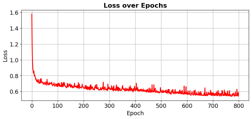
Training is performed for 800 epochs using stochastic gradient descent (SGD) with momentum (0.9) and weight decay (). The learning rate follows a composite schedule consisting of linear warm-up followed by cosine annealing, with automatic scaling according to the effective batch size (256). Mixed-precision training and synchronized batch normalization are employed to improve stability and efficiency. Data augmentation is based on a multi-crop strategy producing two spatial views of size , using random resized cropping with scale range The loss decreases from approximately 1.6 to a stable plateau around 0.6 over training (Figure A2). We trained the DL model on the European Weather Cloud [122] infrastructure equipped with an NVIDIA RTX A6000 GPU (48 GB memory) and an AMD EPYC CPU (16 cores). An 800-epochs long training required approximately 60 hours.
Figure A2.
Training loss over training epochs, computed as the cross-entropy averaged over all batches in each epoch.
Figure A2.
Training loss over training epochs, computed as the cross-entropy averaged over all batches in each epoch.
Appendix D. Cloud Classes Spatial Distribution
Figure A3.
Spatial distribution of crops across the domain for all classes obtained from trining dataset: CS (a), SC (b), MC1 (c), MC2 (d), EC (e), DC (f), OA (g). Crop frequency is computed by aggregating crop occurrences onto a 0.2° × 0.2° latitude–longitude grid. For each grid cell, we count how many crop centers fall within the cell and normalize by the total number of samples per class and dataset. To account for the spatial extent of the crops, the domain is appropriately padded and cropped.
Figure A3.
Spatial distribution of crops across the domain for all classes obtained from trining dataset: CS (a), SC (b), MC1 (c), MC2 (d), EC (e), DC (f), OA (g). Crop frequency is computed by aggregating crop occurrences onto a 0.2° × 0.2° latitude–longitude grid. For each grid cell, we count how many crop centers fall within the cell and normalize by the total number of samples per class and dataset. To account for the spatial extent of the crops, the domain is appropriately padded and cropped.
Appendix E. Pathway Construction and Trajectory Classification
Appendix E.1. Construction of Possible Pathways
We selected three principal classes associated with extreme convective events: EC, DC, and OA. These classes represent the dominant convective regimes identified within the classification framework. Given three classes, we enumerated all theoretically possible ordered pathways up to length three. The pathway set includes:
- Persistence pathways (length 2, same state): EC→EC, DC→DC, OA→OA.
- Binary pathways (length 2, different states): all ordered pairs of distinct classes (6 combinations).
-
Trinary pathways (length 3):
- –
- Triplets with identical initial and final states and a different middle state (6 combinations).
- –
- Triplets with distinct initial and final states and a third intermediate class (6 combinations).
In total, this results in 3 (persistence) + 6 (binary) + 12 (trinary) = 21 possible pathways. Higher-order loops (e.g. pathways longer than three states) were intentionally excluded to reduce interpretational ambiguity and to limit the influence of short-term oscillations potentially arising from classification uncertainty or minor tracking inconsistencies.
Appendix E.2. Trajectory quality control
Storm trajectories were originally constructed at 15-minute temporal resolution. Because missing timestamps can introduce artificial transitions or spurious pathway structures, we applied a strict temporal continuity criteria.
Trajectories containing gaps in the 15-minute time series were excluded to ensure consistent transition detection. From an initial total of 972 trajectories, we removed 85 due to temporal discontinuities, leaving 887 trajectories.
Then, trajectories that did not contain any of the three main classes were removed. These cases correspond to events outside the scope of extreme convective regimes, marginal or ambiguous classifications, or rare configurations that are not relevant to the present pathway framework. This step removed 10 additional trajectories, leaving 877.
Finally, because the pathway analysis was restricted to a maximum of three distinct principal classes, trajectories exhibiting more complex sequences were excluded. This resulted in the removal of 3 additional trajectories.
The final dataset used for pathway analysis consists of 874 trajectories.
Appendix E.3. Pathway Matching Procedure
For each trajectory, we assign a pathway as follows:
- 1.
- Filtering of states: All states not belonging to the three principal classes (EC, DC, OA) were removed.
- 2.
- Collapse of consecutive repetitions: Consecutive identical states were merged into a single occurrence. For example, EC→EC→DC→DC→OA becomes EC→DC→OA. This produces an ordered list of principal classes visited at least once, independent of persistence duration.
- 3.
-
Pathway comparison: The resulting ordered sequence was compared against the predefined set of 21 pathways:
- If only one class remained, the trajectory was classified as persistence.
- If two distinct classes remained, the trajectory was classified as binary.
- If three ordered classes remained, the trajectory was classified as trinary.
Because the definitions of the pathways were mutually exclusive by construction (based on the number of distinct principal classes present), each path was assigned to only one category of pathways.
References
- Grazzini, F.; Fragkoulidis, G.; Teubler, F.; Wirth, V.; Craig, G.C. Extreme precipitation events over northern Italy. Part II: Dynamical precursors. Q. J. R. Meteorol. Soc. 2021, 147, 1237–1257. [Google Scholar] [CrossRef]
- Lombardo, K.; Bitting, M. A Climatology of Convective Precipitation over Europe. Mon. Weather Rev. 2024, 152, 1555–1585. [Google Scholar] [CrossRef]
- Punge, H.J.; Bedka, K.; Kunz, M. A new physically based stochastic event catalog for hail in Europe. Nat. Hazards 2014, 73, 1625–1645. [Google Scholar] [CrossRef]
- Battaglioli, F.; Groenemeijer, P.; Púčik, T.; Taszarek, M.; Ulbrich, U.; Rust, H. Modeled Multidecadal Trends of Lightning and (Very) Large Hail in Europe and North America (1950–2021). J. Appl. Meteorol. Climatol. 2023, 62, 1627–1653. [Google Scholar] [CrossRef]
- Gobiet, A.; Kotlarski, S.; Beniston, M.; Heinrich, G.; Rajczak, J.; Stoffel, M. 21st century climate change in the European Alps—A review. Sci. Total Environ. 2014, 493, 1138–1151. [Google Scholar] [CrossRef] [PubMed]
- Rädler, A.; Groenemeijer, P.; Faust, E.; Sausen, R.; Púčik, T. Frequency of severe thunderstorms across Europe expected to increase in the 21st century due to rising instability. npj Clim. Atmos. Sci. 2019, 2, 1–5. [Google Scholar] [CrossRef]
- Wilhelm, B.; Rapuc, W.; Amann, B.; Anselmetti, F.S.; Arnaud, F.; Blanchet, J.; Brauer, A.; Czymzik, M.; Giguet-Covex, C.; Gilli, A.; et al. Impact of warmer climate periods on flood hazard in the European Alps. Nat. Geosci. 2022, 15, 118–123. [Google Scholar] [CrossRef]
- Hentgen, L.; Ban, N.; Kröner, N.; Leutwyler, D.; Schär, C. Clouds in Convection-Resolving Climate Simulations Over Europe. J. Geophys. Res. Atmos. 2019, 124. [Google Scholar] [CrossRef]
- Henderson, D.; Otkin, J.; Mecikalski, J. Evaluating Convective Initiation in High-Resolution Numerical Weather Prediction Models Using GOES-16 Infrared Brightness Temperatures. Mon. Weather Rev. 2021, 149. [Google Scholar] [CrossRef]
- Fischer, J.; Groenemeijer, P.; Holzer, A.; Feldmann, M.; Schröer, K.; Battaglioli, F.; Schielicke, L.; Púčik, T.; Antonescu, B.; Gatzen, C.; et al. Invited perspectives: Thunderstorm intensification from mountains to plains. Nat. Hazards Earth Syst. Sci. 2025, 25, 2629–2656. [Google Scholar] [CrossRef]
- Panosetti, D.; Böing, S.; Schlemmer, L.; Schmidli, J. Idealized Large-Eddy and Convection-Resolving Simulations of Moist Convection over Mountainous Terrain. J. Atmos. Sci. 2016, 73, 4021–4041. [Google Scholar] [CrossRef]
- Velasquez, P.; Messmer, M.; Raible, C.C. A new bias-correction method for precipitation over complex terrain suitable for different climate states: a case study using WRF (version 3.8.1). Geosci. Model Dev. 2020, 13, 5007–5027. [Google Scholar] [CrossRef]
- De Lucia, C.; Bucchignani, E.; Mastellone, A.; Adinolfi, M.; Montesarchio, M.; Cinquegrana, D.; Mercogliano, P.; Schiano, P. A Sensitivity Study on High Resolution NWP ICON—LAM Model over Italy. Atmosphere 2022, 13. [Google Scholar] [CrossRef]
- Correa-Sánchez, N.; Dallan, E.; Marra, F.; Fosser, G.; Borga, M. Orographic control on bias and uncertainty in extreme sub-daily precipitation simulations from a convection-permitting ensemble. J. Hydrol. 2025, 659, 133324. [Google Scholar] [CrossRef]
- Moncrieff, M.W. The Multiscale Organization of Moist Convection and the Intersection of Weather and Climate. In Climate Dynamics: Why Does Climate Vary? American Geophysical Union (AGU), 2010; pp. 3–26. [Google Scholar] [CrossRef]
- Prein, A.F.; Langhans, W.; Fosser, G.; Ferrone, A.; Ban, N.; Goergen, K.; Keller, M.; Tölle, M.; Gutjahr, O.; Feser, F.; et al. A review on regional convection-permitting climate modeling: Demonstrations, prospects, and challenges. Rev. Geophys. 2015, 53, 323–361. [Google Scholar] [CrossRef]
- Volkert, H.; Gutermann, T. Inter-domain cooperation for mesoscale atmospheric laboratories: The mesoscale Alpine programme as a rich study case. Q. J. R. Meteorol. Soc. 2007, 133, 949–967. [Google Scholar] [CrossRef]
- Khodayar, S.; Davolio, S.; Di Girolamo, P.; Lebeaupin Brossier, C.; Flaounas, E.; Fourrie, N.; Lee, K.O.; Ricard, D.; Vie, B.; Bouttier, F.; et al. Overview towards improved understanding of the mechanisms leading to heavy precipitation in the western Mediterranean: lessons learned from HyMeX. Atmos. Chem. Phys. 2021, 21, 17051–17078. [Google Scholar] [CrossRef]
- Handwerker, J.; Barthlott, C.; Bauckholt, M.; Belleflamme, A.; Böhmländer, A.; Borg, E.; Dick, G.; Dietrich, P.; Fichtelmann, B.; Geppert, G.; et al. From initiation of convective storms to their impact — the Swabian MOSES 2023 campaign in southwestern Germany. Front. Earth Sci. 2025, 13. [Google Scholar] [CrossRef]
- Serafin, S.; Rotach, M.W.; Arpagaus, M.; Colfescu, I.; Cuxart, J.; De Wekker, S.F.J.; Evans, M.; Grubišić, V.; Kalthoff, N.; Karl, T.; et al. Multi-scale transport and exchange processes in the atmosphere over mountains: Programme and experiment. Report; Innsbruck University Press: Innsbruck, Austria, 2020. [Google Scholar] [CrossRef]
- Rotach, M.W.; Serafin, S.; Ward, H.C.; Arpagaus, M.; Colfescu, I.; Cuxart, J.; Wekker, S.F.J.D.; Grubišic, V.; Kalthoff, N.; Karl, T.; et al. A Collaborative Effort to Better Understand, Measure, and Model Atmospheric Exchange Processes over Mountains. Bull. Am. Meteorol. Soc. 2022, 103, E1282–E1295. [Google Scholar] [CrossRef]
- Avolio, E.; Nisi, L.; Panziera, L.; Peyraud, L.; Miglietta, M. A multi-sensor and modeling analysis of a severe convective storm in Lake Maggiore area (northwestern Italy). Atmos. Res. 2020, 242, 105008. [Google Scholar] [CrossRef]
- Feldmann, M.; Hering, A.; Gabella, M.; et al. Hailstorms and rainstorms versus supercells—a regional analysis of convective storm types in the Alpine region. npj Clim. Atmos. Sci. 2023, 6, 19. [Google Scholar] [CrossRef]
- Franch, G.; Maggio, V.; Coviello, L.; Pendesini, M.; Jurman, G.; Furlanello, C. TAASRAD19, a high-resolution weather radar reflectivity dataset for precipitation nowcasting. Sci. Data 2020, 7. [Google Scholar] [CrossRef] [PubMed]
- Nisi, L.; Hering, A.; Germann, U.; Schröer, K.; Barras, H.; Kunz, M.; Martius, O. Hailstorms in the Alpine region: Diurnal cycle, 4D-characteristics, and the nowcasting potential of lightning properties. Q. J. R. Meteorol. Soc. 2020, 146. [Google Scholar] [CrossRef]
- Germann, U.; Boscacci, M.; Clementi, L.; Gabella, M.; Hering, A.; Sartori, M.; Sideris, I.V.; Calpini, B. Weather Radar in Complex Orography. Remote Sens. 2022, 14. [Google Scholar] [CrossRef]
- Borga, M.; Marra, F.; Gabella, M. Chapter 5 - Rainfall estimation by weather radar. In Rainfall; Morbidelli, R., Ed.; Elsevier, 2022; pp. 109–134. [Google Scholar] [CrossRef]
- Ohara, K.; Masunaga, H. Synergy of millimeter-wave radar and radiometer measurements for retrieving frozen hydrometeors in deep convective systems. Atmos. Meas. Tech. 2025, 18, 4791–4807. [Google Scholar] [CrossRef]
- Roh, W.; Satoh, M.; Matsugishi, S.; Aoki, S.; Kubota, T.; Okamoto, H. Vertical motions in clouds from EarthCare satellite and a global storm-resolving modeling. Sci. Rep. 2025, 16. [Google Scholar] [CrossRef] [PubMed]
- Cattani, E.; Torricella, F.; Laviola, S.; Levizzani, V. On the statistical relationship between cloud optical and microphysical characteristics and rainfall intensity for convective storms over the Mediterranean. Nat. Hazards Earth Syst. Sci. 2009, 9, 2135–2142. [Google Scholar] [CrossRef]
- Skofronick-Jackson, G.; Kirschbaum, D.; Petersen, W.; Huffman, G.; Kidd, C.; Stocker, E.; Kakar, R. The Global Precipitation Measurement (GPM) mission’s scientific achievements and societal contributions: reviewing four years of advanced rain and snow observations. Q. J. R. Meteorol. Soc. 2018, 144, 27–48. [Google Scholar] [CrossRef] [PubMed]
- Levizzani, V.; Cattani, E. Satellite Remote Sensing of Precipitation and the Terrestrial Water Cycle in a Changing Climate. Remote Sens. 2019, 11. [Google Scholar] [CrossRef]
- Mroz, K.; Battaglia, A.; Lang, T.J.; Cecil, D.J.; Tanelli, S.; Tridon, F. Hail-Detection Algorithm for the GPM Core Observatory Satellite Sensors. J. Appl. Meteorol. Climatol. 2017, 56, 1939–1957. [Google Scholar] [CrossRef]
- Laviola, S.; Monte, G.; Cattani, E.; Levizzani, V. Hail Climatology in the Mediterranean Basin Using the GPM Constellation (1999–2021). Remote Sens. 2022, 14. [Google Scholar] [CrossRef]
- Mecikalski, J.; MacKenzie, W.; Koenig, M.; Muller, S. Cloud-Top Properties of Growing Cumulus prior to Convective Initiation as Measured by Meteosat Second Generation. Part II: Use of Visible Reflectance. J. Appl. Meteorol. Climatol. 2010, 49, 2544–2558. [Google Scholar] [CrossRef]
- Mecikalski, J.R.; MacKenzie, W.M.; Koenig, M.; Muller, S. Cloud-Top Properties of Growing Cumulus prior to Convective Initiation as Measured by Meteosat Second Generation. Part I: Infrared Fields. J. Appl. Meteorol. Climatol. 2010, 49, 521–534. [Google Scholar] [CrossRef]
- Cattani, E.; Melani, S.; Levizzani, V.; Costa, M.J. The Retrieval of Cloud Top Properties Using VIS-IR Channels. Meas. Precip. From Space-EURAINSAT Future 2006, 79–95. [Google Scholar] [CrossRef]
- Mecikalski, J.R.; Bedka, K.M. Forecasting Convective Initiation by Monitoring the Evolution of Moving Cumulus in Daytime GOES Imagery. Mon. Weather Rev. 2006, 134, 49–78. [Google Scholar] [CrossRef]
- Mecikalski, J.R.; Williams, J.K.; Jewett, C.P.; Ahijevych, D.; LeRoy, A.; Walker, J.R. Probabilistic 0–1-h Convective Initiation Nowcasts that Combine Geostationary Satellite Observations and Numerical Weather Prediction Model Data. J. Appl. Meteorol. Climatol. 2015, 54, 1039–1059. [Google Scholar] [CrossRef]
- Mecikalski, J.; Rosenfeld, D.; Manzato, A. Evaluation of Geostationary Satellite Observations and the Development of a 1-2 hour Prediction Model for Future Storm Intensity: Forecasting Storm Intensity. J. Geophys. Res. Atmos. 2016, 121. [Google Scholar] [CrossRef]
- Merino, A.; López, L.; Sánchez, J.L.; García-Ortega, E.; Cattani, E.; Levizzani, V. Daytime identification of summer hailstorm cells from MSG data. Nat. Hazards Earth Syst. Sci. 2014, 14, 1017–1033. [Google Scholar] [CrossRef]
- Kotarba, A.Z.; Wojciechowska, I. Satellite-based detection of deep-convective clouds: the sensitivity of infrared methods and implications for cloud climatology. Atmos. Meas. Tech. 2025, 18, 2721–2738. [Google Scholar] [CrossRef]
- Galfione, A.; Battaglia, A.; Oue, M.; Cattani, E.; Kollias, P. Comparison of GOES16 Data with the TRACER-ESCAPE Field Campaign Dataset for Convection Characterization: A Selection of Case Studies and Lessons Learnt. Remote Sens. 2025, 17. [Google Scholar] [CrossRef]
- Levizzani, V.; Pinelli, F.; Pasqui, M.; Melani, S.; Laing, A.G.; Carbone, R.E. A 10-year climatology of warm-season cloud patterns over Europe and the Mediterranean from Meteosat IR observations. Atmos. Res. 2010, 97, 555–576. [Google Scholar] [CrossRef]
- Henken, C.; Schmeits, M.; Deneke, H.; Roebeling, R. Using MSG-SEVIRI Cloud Physical Properties and Weather Radar Observations for the Detection of Cb/TCu Clouds. J. Appl. Meteorol. Climatol. 2011, 50, 1587–1600. [Google Scholar] [CrossRef]
- Cintineo, J.L.; Pavolonis, M.J.; Sieglaff, J.M.; Heidinger, A.K. Evolution of Severe and Nonsevere Convection Inferred from GOES-Derived Cloud Properties. J. Appl. Meteorol. Climatol. 2013, 52, 2009–2023. [Google Scholar] [CrossRef]
- Keller, M.; Fuhrer, O.; Schmidli, J.; Stengel, M.; Stöckli, R.; Schär, C. Evaluation of convection-resolving models using satellite data: The diurnal cycle of summer convection over the Alps. Meteorol. Z. 2016, 25, 165–179. [Google Scholar] [CrossRef]
- Senf, F.; Deneke, H. Satellite-Based Characterization of Convective Growth and Glaciation and Its Relationship to Precipitation Formation over Central Europe. J. Appl. Meteorol. Climatol. 2017, 56, 1827–1845. [Google Scholar] [CrossRef]
- Xu, Y.; Sun, K.; Lv, F.; Bian, Z.; Zhou, X.; Miao, S.; He, T. Identification of severe convective clouds and analysis of their relationship with severe convective weather based on Himawari-8/9 geostationary satellite. Atmos. Res. 2026, 327, 108349. [Google Scholar] [CrossRef]
- Anderson, S.R.; Cole, S.J.; Klein, C.; Taylor, C.M.; Diop, C.A.; Kamara, M. Nowcasting convective activity for the Sahel: A simple probabilistic approach using real-time and historical satellite data on cloud-top temperature. Q. J. R. Meteorol. Soc. 2024, 150, 597–617. [Google Scholar] [CrossRef]
- Afzali Gorooh, V.; Delle Monache, L.; Axisa, D.; Sengupta, A.; Zhang, Z.; Ralph, F. Deterministic nowcasting of geostationary satellite infrared brightness temperature using 3D U-Net diffusion model. Sci. Rep. 2026, 16. [Google Scholar] [CrossRef] [PubMed]
- Bedka, K.; Brunner, J.; Dworak, R.; Feltz, W.; Otkin, J.; Greenwald, T. Objective Satellite-Based Detection of Overshooting Tops Using Infrared Window Channel Brightness Temperature Gradients. J. Appl. Meteorol. Climatol. 2010, 49, 181–202. [Google Scholar] [CrossRef]
- Bedka, K.M.; Dworak, R.; Brunner, J.; Feltz, W. Validation of Satellite-Based Objective Overshooting Cloud-Top Detection Methods Using CloudSat Cloud Profiling Radar Observations. J. Appl. Meteorol. Climatol. 2012, 51, 1811–1822. [Google Scholar] [CrossRef]
- Griffin, S.M.; Bedka, K.M.; Velden, C.S. A Method for Calculating the Height of Overshooting Convective Cloud Tops Using Satellite-Based IR Imager and CloudSat Cloud Profiling Radar Observations. J. Appl. Meteorol. Climatol. 2016, 55, 479–491. [Google Scholar] [CrossRef]
- Coopman, Q.; Hoose, C.; Stengel, M. Analysis of the Thermodynamic Phase Transition of Tracked Convective Clouds Based on Geostationary Satellite Observations. J. Geophys. Res. Atmos. 2020, 125, e2019JD032146. [Google Scholar] [CrossRef]
- Mecikalski, J.R.; Minnis, P.; Palikonda, R. Use of satellite derived cloud properties to quantify growing cumulus beneath cirrus clouds. Atmos. Res. 2013, 120-121, 192–201. [Google Scholar] [CrossRef]
- Rossow, W.B.; Schiffer, R.A. Advances in Understanding Clouds from ISCCP. Bull. Am. Meteorol. Soc. 1999, 80, 2261–2288. [Google Scholar] [CrossRef]
- Benas, N.; Holtermann, I.; Stengel, M.; Hüser, I.; Karlsson, K.G.; Häkansson, N.; Johansson, E.; Eliasson, S.; Schröder, M.; Hollmann, R.; et al. CLAAS-3: the third edition of the CM SAF cloud data record based on SEVIRI observations. Earth Syst. Sci. Data 2023, 15, 5153–5170. [Google Scholar] [CrossRef]
- Morel, C.; Senesi, S. A climatology of mesoscale convective systems over Europe using satellite infrared imagery. II: Characteristics of European mesoscale convective systems. Q. J. R. Meteorol. Soc. 2002, 128, 1973–1995. [Google Scholar] [CrossRef]
- Tzallas, V.; Hünerbein, A.; Stengel, M.; Meirink, J.F.; Benas, N.; Trentmann, J.; Macke, A. CRAAS: A European Cloud Regime dAtAset Based on the CLAAS-2.1 Climate Data Record. Remote Sens. 2022, 14, 5548. [Google Scholar] [CrossRef]
- Cotín, L.; Castro Lobera, M.P. Overview of the EUMETSAT Satellite Application Facility for NoWCasting and Very Short Range Forecasting. In Proceedings of the Conference: SAF Training Workshop. Nowcasting and Veru Short Range Forecasting. INM, Madrid, Spain, 9-11 December 1998, 01 1999. [Google Scholar]
- Visa, A.; Iivarinen, J.; Valkealahti, K.; Simula, O. NEURAL NETWORK BASED CLOUD CLASSIFIER. In Industrial Applications of Neural Networks; World Scientific, 1998; pp. 303–309. [Google Scholar] [CrossRef]
- Christodoulou, C.; Michaelides, S.; Pattichis, C. Multifeature texture analysis for the classification of clouds in satellite imagery. Geosci. Remote Sens. IEEE Trans. 2003, 41, 2662–2668. [Google Scholar] [CrossRef]
- Fu, Y.; Fei, M.; Han, Z.; Zhang, W.; Liu, Q.; Gu, X.; Yu, T. A Machine-Learning-Based Study on All-Day Cloud Classification Using Himawari-8 Infrared Data. Remote Sens. 2023, 15, 5630. [Google Scholar] [CrossRef]
- Guo, B.; Zhang, F.; Li, W.; Zhao, Z. Cloud Classification by Machine Learning for Geostationary Radiation Imager. IEEE Trans. Geosci. Remote Sens. 2024, 62, 1–14. [Google Scholar] [CrossRef]
- Jing, L.; Tian, Y. Self-Supervised Visual Feature Learning With Deep Neural Networks: A Survey. IEEE Trans. Pattern Anal. Mach. Intell. 2021, 43, 4037–4058. [Google Scholar] [CrossRef] [PubMed]
- Lee, Y.; Kummerow, C.; Ebert-Uphoff, I. Applying machine learning methods to detect convection using Geostationary Operational Environmental Satellite-16 (GOES-16) advanced baseline imager (ABI) data. Atmos. Meas. Tech. 2021, 14, 2699–2716. [Google Scholar] [CrossRef]
- Kaps, A.; Lauer, A.; Kazeroni, R.; Stengel, M.; Eyring, V. Characterizing clouds with the CCClim dataset, a machine learning cloud class climatology. Earth Syst. Sci. Data 2024, 16, 3001–3016. [Google Scholar] [CrossRef]
- Kim, M.; Lee, J.; Im, J. Deep Learning-based Monitoring of Overshooting Cloud Tops from Geostationary Satellite Data. GIScience Remote Sens. 2018, 55. [Google Scholar] [CrossRef]
- Han, D.; Lee, J.; Im, J.; Sim, S.; Lee, S.; Han, H. A Novel Framework of Detecting Convective Initiation Combining Automated Sampling, Machine Learning, and Repeated Model Tuning from Geostationary Satellite Data. Remote Sens. 2019, 11. [Google Scholar] [CrossRef]
- Cintineo, J.L.; Pavolonis, M.J.; Sieglaff, J.M.; Wimmers, A.; Brunner, J.; Bellon, W. A Deep-Learning Model for Automated Detection of Intense Midlatitude Convection Using Geostationary Satellite Images. Weather Forecast. 2020, 35, 2567–2588. [Google Scholar] [CrossRef]
- Lenhardt, J.; Quaas, J.; Sejdinovic, D.; Klocke, D. CloudViT: exploring cloud type classification with vision transformers in global satellite data. Atmos. Chem. Phys. 2026, 26, 5447–5475. [Google Scholar] [CrossRef]
- Fan, D.; Greybush, S.J.; Clothiaux, E.E.; Gagne, D.J. Physically Explainable Deep Learning for Convective Initiation Nowcasting Using GOES-16 Satellite Observations. Artif. Intell. Earth Syst. 2024, 3, e230098. [Google Scholar] [CrossRef]
- Brüning, S.; Tost, H. A machine-learning-based perspective on deep convective clouds and their organisation in 3D – Part 1: Influence of deep convective cores on the cloud life cycle. Atmos. Chem. Phys. 2025, 25, 10773–10795. [Google Scholar] [CrossRef]
- Brüning, S.; Tost, H. A machine-learning-based perspective on deep convective clouds and their organisation in 3D – Part 2: Spatial–temporal patterns of convective organisation. Atmos. Chem. Phys. 2025, 25, 10797–10822. [Google Scholar] [CrossRef]
- Kim, D.; Kim, H.J.; Choi, Y.S. Unsupervised Clustering of Geostationary Satellite Cloud Properties for Estimating Precipitation Probabilities of Tropical Convective Clouds. J. Appl. Meteorol. Climatol. 2023, 62, 1083–1094. [Google Scholar] [CrossRef]
- Denby, L. Discovering the Importance of Mesoscale Cloud Organization Through Unsupervised Classification. Geophys. Res. Lett. 2020, 47, e2019GL085190. [Google Scholar] [CrossRef]
- Denby, L. Charting the Realms of Mesoscale Cloud Organisation using Unsupervised Learning; 2023. [Google Scholar]
- Kurihana, T.; Moyer, E.; Willett, R.; Gilton, D.; Foster, I. Data-Driven Cloud Clustering via a Rotationally Invariant Autoencoder. IEEE Trans. Geosci. Remote Sens. 2022, 60, 1–25. [Google Scholar] [CrossRef]
- Hendrycks, D.; Mazeika, M.; Kadavath, S.; Song, D. Using Self-Supervised Learning Can Improve Model Robustness and Uncertainty. In Proceedings of the Advances in Neural Information Processing Systems; 2019; Vol. 33, pp. 15663–15674, NeurIPS 2019. [Google Scholar]
- Liu, H.; HaoChen, J.; Gaidon, A.; Ma, T. Self-supervised Learning is More Robust to Dataset Imbalance, 2021. Preprint. [CrossRef]
- Chatterjee, D.; Acquistapace, C.; Deneke, H.; Crewell, S. Understanding Cloud Systems’ Structure and Organization Using a Machine’s Self-Learning Approach. Artif. Intell. Earth Syst. 2023, 2. [Google Scholar] [CrossRef]
- Chatterjee, D.; Raabe, N.; Crewell, S. Four low-level cloud regimes revealed by latent space analysis and their impact on solar energy variability. Mach. Learn. Earth 2026, 2, 015015. [Google Scholar] [CrossRef]
- Geiss, A.; Christensen, M.; Varble, A.; Yuan, T.; Song, H. Self Supervised Cloud Classification. Artif. Intell. Earth Syst. 2023, 3. [Google Scholar] [CrossRef]
- Chatterjee, D.; Schnitt, S.; Bigalke, P.; Acquistapace, C.; Crewell, S. Capturing the Diversity of Mesoscale Trade Wind Cumuli Using Complementary Approaches From Self-Supervised Deep Learning. Geophys. Res. Lett. 2024, 51, e2024GL108889. [Google Scholar] [CrossRef]
- Yan, W.; Xiong, X.; Xia, X.; Zhang, Y.; Guo, X. Self-Supervised Cloud Classification with Patch Rotation Tasks (SSCC-PR). Appl. Sci. 2025, 15, 9051. [Google Scholar] [CrossRef]
- Lv, Q.; Li, Q.; Chen, K.; Lu, Y.; Wang, L. Classification of Ground-Based Cloud Images by Contrastive Self-Supervised Learning. Remote Sens. 2022, 14. [Google Scholar] [CrossRef]
- Dotzek, N.; Groenemeijer, P.; Feuerstein, B.; Holzer, A. Overview of ESSL’s severe convective storms research using the European Severe Weather Database ESWD. Atmos. Res. 2009, 93, 575–586. [Google Scholar] [CrossRef]
- Schumacher, R.; Rasmussen, K. The formation, character and changing nature of mesoscale convective systems. Nat. Rev. Earth Environ. 2020, 1, 1–15. [Google Scholar] [CrossRef]
- Schmetz, J.; Pili, P.; Tjemkes, S.; Just, D.; Kerkmann, J.; Rota, S.; Ratier, A. An introduction to Meteosat Second Generation (MSG). Bull. Amer. Meteor. Soc. 2002, 83, 977–992. [Google Scholar] [CrossRef]
- Karlsson, K.G.; Johansson, E.; Häkansson, N.; Sedlar, J.; Eliasson, S. Probabilistic Cloud Masking for the Generation of CM SAF Cloud Climate Data Records from AVHRR and SEVIRI Sensors. Remote Sens. 2020, 12, 713. [Google Scholar] [CrossRef]
- Huffman, G.J.; Bolvin, D.T.; Braithwaite, D.; Hsu, K.L.; Joyce, R.J.; Kidd, C.; Nelkin, E.J.; Sorooshian, S.; Stocker, E.F.; Tan, J.; et al. Integrated Multi-satellite Retrievals for the Global Precipitation Measurement (GPM) Mission (IMERG). In Satellite Precipitation Measurement; Levizzani, V., Kidd, C., Kirschbaum, D.B., Kummerow, C.D., Nakamura, K., Turk, F.J., Eds.; Springer International Publishing: Cham, 2020; Volume 1, pp. 343–353. [Google Scholar] [CrossRef]
- Navarro, A.; García-Ortega, E.; Merino, A.; Sánchez, J.L.; Kummerow, C.; Tapiador, F.J. Assessment of IMERG Precipitation Estimates over Europe. Remote Sens. 2019, 11. [Google Scholar] [CrossRef]
- Goyal, P.; Duval, Q.; Reizenstein, J.; Leavitt, M.; Xu, M.; Lefaudeux, B.; Singh, M.; Reis, V.; Caron, M.; Bojanowski, P.; et al. VISSL. 2021. Available online: https://github.com/facebookresearch/vissl.
- Caron, M.; Misra, I.; Mairal, J.; Goyal, P.; Bojanowski, P.; Joulin, A. Unsupervised Learning of Visual Features by Contrasting Cluster Assignments. In Proceedings of the Advances in Neural Information Processing Systems; Larochelle, H., Ranzato, M., Hadsell, R., Balcan, M., Lin, H., Eds.; Curran Associates, Inc., 2020; Vol. 33, pp. 9912–9924. [Google Scholar]
- He, K.; Zhang, X.; Ren, S.; Sun, J. Deep Residual Learning for Image Recognition. In Proceedings of the 2016 IEEE Conference on Computer Vision and Pattern Recognition (CVPR), 2016; pp. 770–778. [Google Scholar] [CrossRef]
- Hornik, K.; Feinerer, I.; Kober, M.; Buchta, C. Spherical k-Means Clustering. J. Stat. Softw. 2012, 50, 1–22. [Google Scholar] [CrossRef]
- van der Maaten, L.; Hinton, G. Visualizing Data using t-SNE. J. Mach. Learn. Res. 2008, 9, 2579–2605. [Google Scholar]
- Houze, R.A. Cloud Dynamics, 2 ed.; Academic Press: Oxford, 2014. [Google Scholar]
- Miglietta, M.; Davolio, S. Dynamical forcings in heavy precipitation events over Italy: lessons from the HyMeX SOP1 campaign. Hydrol. Earth Syst. Sci. 2022, 26, 627–646. [Google Scholar] [CrossRef]
- Feldmann, M.; Domeisen, D.I.V.; Martius, O. A pan-European analysis of large-scale drivers of severe convective outbreaks. Weather Clim. Dyn. 2025, 6, 1089–1106. [Google Scholar] [CrossRef]
- Roca, R.; Fiolleau, T.; Bouniol, D. A Simple Model of the Life Cycle of Mesoscale Convective Systems Cloud Shield in the Tropics. J. Clim. 2017, 30, 4283–4298. [Google Scholar] [CrossRef]
- Schaffer, A.; Lichtenegger, T.; Truhetz, H.; Ossó, A.; Martínez-Alvarado, O.; Maraun, D. Drivers of Cold Frontal Hourly Extreme Precipitation: A Climatological Study Over Europe. Geophys. Res. Lett. 2024, 51, e2024GL111025. [Google Scholar] [CrossRef]
- Da Silva, N.; Haerter, J. The Precipitation Characteristics of Mesoscale Convective Systems Over Europe. J. Geophys. Res. Atmos. 2023, 128, e2023JD039045. [Google Scholar] [CrossRef]
- Taszarek, M.; Allen, J.T.; Groenemeijer, P.; Edwards, R.; Brooks, H.E.; Chmielewski, V.; Enno, S.E. Severe Convective Storms across Europe and the United States. Part I: Climatology of Lightning, Large Hail, Severe Wind, and Tornadoes. J. Clim. 2020, 33, 10239–10261. [Google Scholar] [CrossRef]
- Houze, R.A., Jr. Mesoscale convective systems. Rev. Geophys. 2004, 42. [Google Scholar] [CrossRef]
- Houze, R. Orographic effects on precipitating clouds. Rev. Geophys. 2012, 50, 1001. [Google Scholar] [CrossRef]
- Nisi, L.; Ambrosetti, P.; Clementi, L. Nowcasting severe convection in the Alpine region: the COALITION approach. Q. J. R. Meteorol. Soc. 2013, 140, 1684–1699. [Google Scholar] [CrossRef]
- De Martin, F.; Manzato, A.; Carlon, N.; Setvák, M.; Miglietta, M.M. Dynamic and statistical analysis of giant hail environments in northeast Italy. Q. J. R. Meteorol. Soc. 2025, 151, e4945. [Google Scholar] [CrossRef]
- Groot, E.; Kuntze, P.; Miltenberger, A.; Tost, H. Divergent convective outflow in ICON deep-convection-permitting and parameterised deep convection simulations. Weather Clim. Dyn. 2024, 5, 779–803. [Google Scholar] [CrossRef]
- Davolio, S.; Buzzi, A.; Malguzzi, P. Orographic triggering of long lived convection in three dimensions. Meteorol. Atmos. Phys. 2009, 103, 35–44. [Google Scholar] [CrossRef]
- Davolio, S.; Mastrangelo, D.; Miglietta, M.M.; Drofa, O.; Buzzi, A.; Malguzzi, P. High resolution simulations of a flash flood near Venice. Nat. Hazards Earth Syst. Sci. 2009, 9, 1671–1678. [Google Scholar] [CrossRef]
- Degiacomi, T.; Zonato, A.; Davolio, S.; Miglietta, M.M.; Giovannini, L. Deep Banded Orographic Convection over an Idealized Mountain Range: Influence of Upstream Atmospheric Conditions. J. Atmos. Sci. 2025, 82, 1033–1055. [Google Scholar] [CrossRef]
- Fischer, J.; Kunz, M.; Lombardo, K.; Kumjian, M.R. Hail Trajectories in a Wide Spectrum of Supercell-Like Updrafts. J. Atmos. Sci. 2025, 82, 1403–1422. [Google Scholar] [CrossRef]
- Li, Q.; Shi, H.; Xie, Y.; Jiang, R.; Wang, C.; Teng, Y.; Jia, S.; Wen, J.; Fu, D.; Yang, J.; et al. Revealing the lifecycle evolution of hail-producing deep convective clouds by synergy of multi-source data. Atmos. Res. 2026, 336, 108845. [Google Scholar] [CrossRef]
- Tselioudis, G.; Rossow, W.; Zhang, Y.; Konsta, D. Global Weather States and Their Properties from Passive and Active Satellite Cloud Retrievals. J. Clim. 2013, 26, 7734–7746. [Google Scholar] [CrossRef]
- Oreopoulos, L.; Cho, N.; Lee, D.; Kato, S.; Huffman, G.J. An examination of the nature of global MODIS cloud regimes. J. Geophys. Res. Atmos. 2014, 119, 8362–8383. [Google Scholar] [CrossRef]
- Stubenrauch, C.J.; Rossow, W.B.; Kinne, S.; Ackerman, S.; Cesana, G.; Chepfer, H.; Girolamo, L.D.; Getzewich, B.; Guignard, A.; Heidinger, A.; et al. Assessment of Global Cloud Datasets from Satellites: Project and Database Initiated by the GEWEX Radiation Panel. Bull. Am. Meteorol. Soc. 2013, 94, 1031–1049. [Google Scholar] [CrossRef]
- Crameri, F. Geodynamic diagnostics, scientific visualisation and StagLab 3.0. Geosci. Model Dev. 2018, 11, 2541–2562. [Google Scholar] [CrossRef]
- Deng, D. DBSCAN Clustering Algorithm Based on Density. In Proceedings of the 2020 7th International Forum on Electrical Engineering and Automation (IFEEA), 2020; pp. 949–953. [Google Scholar] [CrossRef]
- Heikenfeld, M.; Marinescu, P.J.; Christensen, M.; Watson-Parris, D.; Senf, F.; van den Heever, S.C.; Stier, P. tobac 1.2: towards a flexible framework for tracking and analysis of clouds in diverse datasets. Geosci. Model Dev. 2019, 12, 4551–4570. [Google Scholar] [CrossRef]
- Tervo, R.; Schulz, J.; Saalmueller, J.; Abellan, X.; Modigliani, U.; Baousis, V. The European Weather Cloud (EWC) – Collaboration Platform for Meteorological Application Development and Data Processing. In Proceedings of the EMS Annual Meeting 2022, Bonn, Germany, 2022; pp. EMS2022–16. [Google Scholar] [CrossRef]
Figure 1.
(a) Elevation map of the Alpine study domain. Training dataset: (b) Example of the random cropping procedure over the Alpine domain. Two randomly positioned 100 × 100 pixel crops (orange frame) are extracted at each timestep from the IR 10.8 μm channel. Black pixels correspond to a BT of 320 K (see colorbar in panel f) and represent clear-sky pixels masked using the cloud mask. In each crop we extract a random pair of image views (pink and light-blue frames). (c) DeepCluster-v2 architecture used for SSL model trained using the two views. Test dataset: (d) Collection of extreme precipitation and hail reports from the ESWD. (e) Aggregation of reports into 15-min intervals and spatial clustering (stars denote cluster centers). (f) Reconstruction of storm trajectories by linking cluster centers across consecutive timestamps, interpolating missing timestamps within 1 hour, and extending trajectories by ±2 h beyond the observation period. Satellite crops (100 × 100 pixels) are then extracted at each cluster centers.
Figure 1.
(a) Elevation map of the Alpine study domain. Training dataset: (b) Example of the random cropping procedure over the Alpine domain. Two randomly positioned 100 × 100 pixel crops (orange frame) are extracted at each timestep from the IR 10.8 μm channel. Black pixels correspond to a BT of 320 K (see colorbar in panel f) and represent clear-sky pixels masked using the cloud mask. In each crop we extract a random pair of image views (pink and light-blue frames). (c) DeepCluster-v2 architecture used for SSL model trained using the two views. Test dataset: (d) Collection of extreme precipitation and hail reports from the ESWD. (e) Aggregation of reports into 15-min intervals and spatial clustering (stars denote cluster centers). (f) Reconstruction of storm trajectories by linking cluster centers across consecutive timestamps, interpolating missing timestamps within 1 hour, and extending trajectories by ±2 h beyond the observation period. Satellite crops (100 × 100 pixels) are then extracted at each cluster centers.
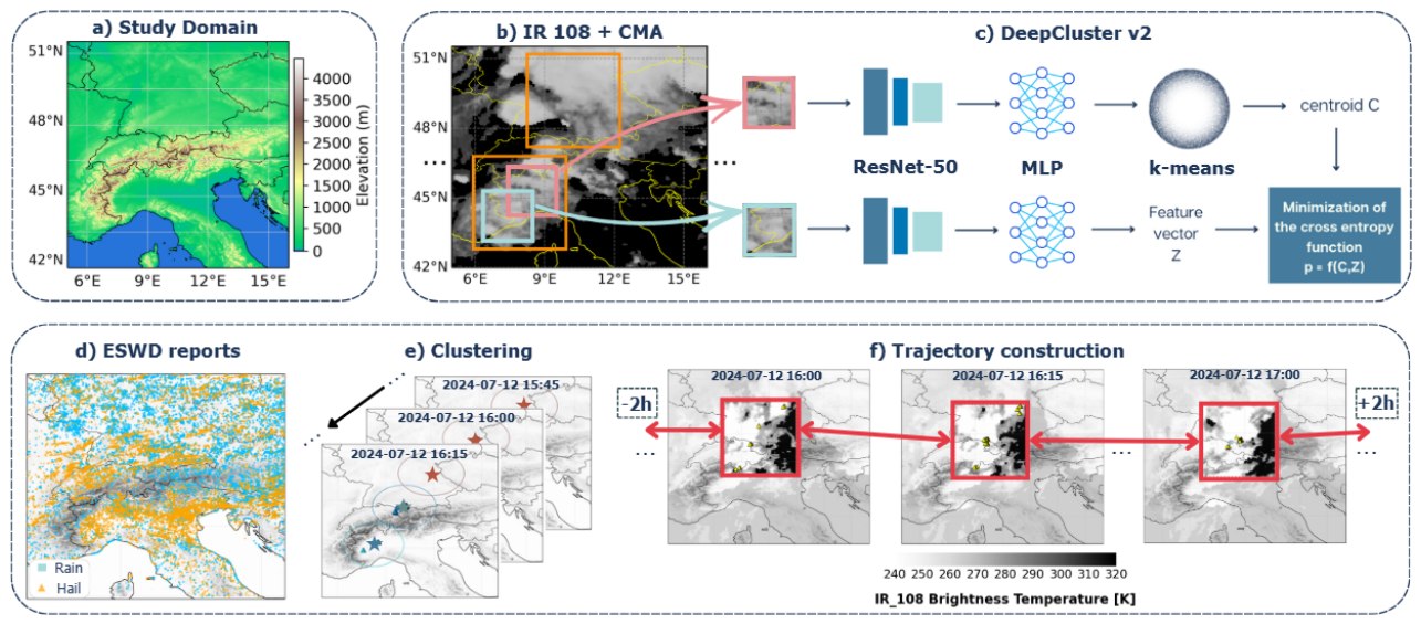
Figure 2.
Visual inspection of the learned feature space after model training. (a) Two-dimensional representation obtained using the t-SNE technique, showing around 300 example of image crops; stars indicate the centroid positions. The crop grid image is created by dividing the feature space into a regular grid, and selecting for each cell the image closest to the cell center. BT 10.8 μm images are reproduced using a greyscale colormap normalized between 240 K and 320 K, which highlights high cloud tops that saturate near 240 K. This IR BT representation is used throughout the text. (b) Example of image crops corresponding to the five samples closest to each class centroid for the seven classes.
Figure 2.
Visual inspection of the learned feature space after model training. (a) Two-dimensional representation obtained using the t-SNE technique, showing around 300 example of image crops; stars indicate the centroid positions. The crop grid image is created by dividing the feature space into a regular grid, and selecting for each cell the image closest to the cell center. BT 10.8 μm images are reproduced using a greyscale colormap normalized between 240 K and 320 K, which highlights high cloud tops that saturate near 240 K. This IR BT representation is used throughout the text. (b) Example of image crops corresponding to the five samples closest to each class centroid for the seven classes.
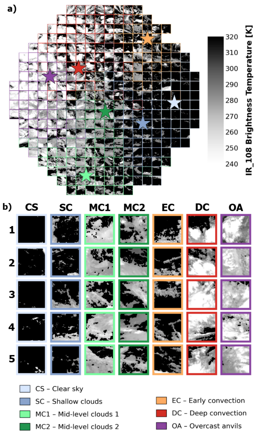
Figure 3.
Physical characterization of the training-set feature space. (a) Number of samples per class, separated into daytime (05-17 UTC) and nighttime (18-04 UTC) observations (hatched). (b) Hourly distribution of samples for each class, shown as stacked bars. (c–e) Boxplot distributions of CC (c), CTHmedian (d), and COTmedian (e) for each class. Classes dominated by nighttime samples may contain fewer data points due to the unavailability of COT retrievals during nighttime conditions.
Figure 3.
Physical characterization of the training-set feature space. (a) Number of samples per class, separated into daytime (05-17 UTC) and nighttime (18-04 UTC) observations (hatched). (b) Hourly distribution of samples for each class, shown as stacked bars. (c–e) Boxplot distributions of CC (c), CTHmedian (d), and COTmedian (e) for each class. Classes dominated by nighttime samples may contain fewer data points due to the unavailability of COT retrievals during nighttime conditions.
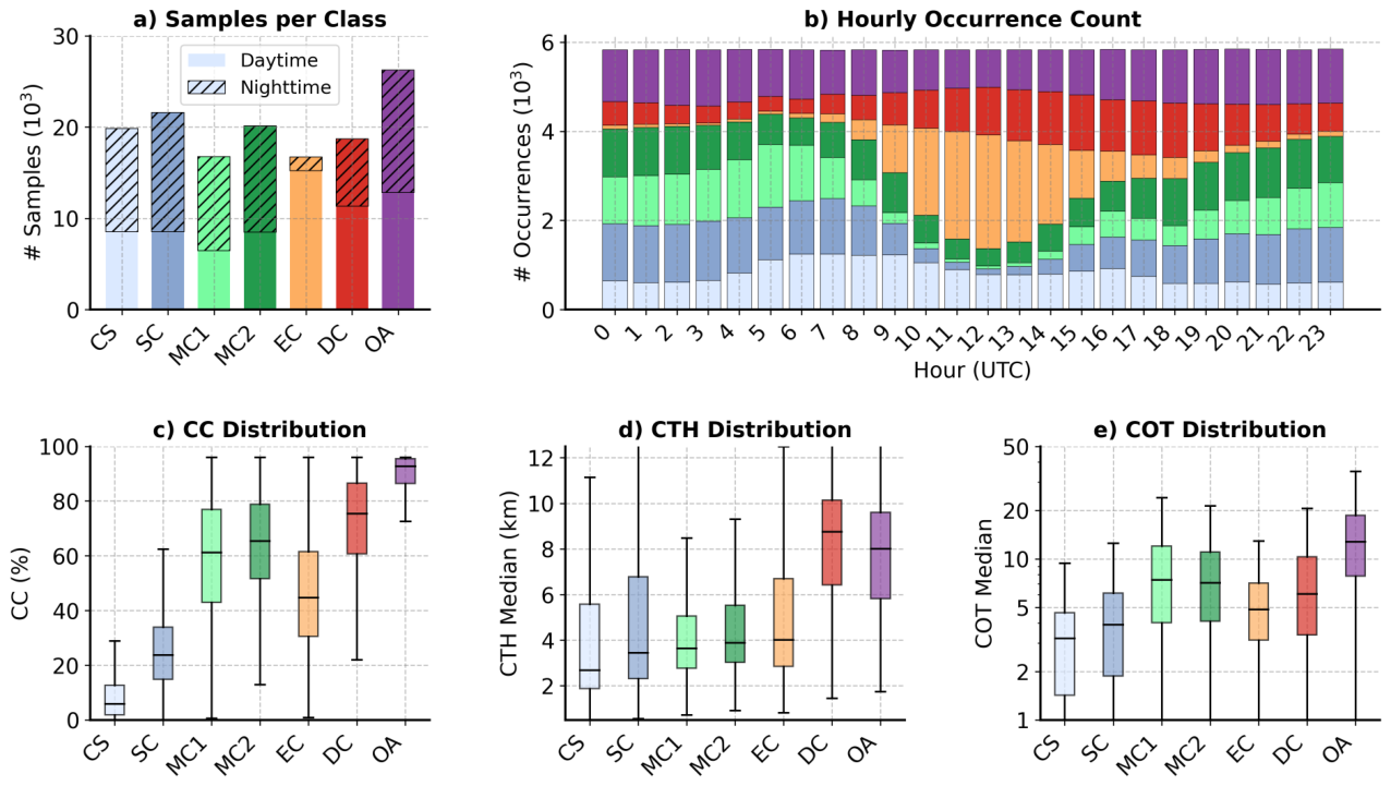
Figure 4.
Feature-space representation of the test dataset. (a) Density contours of test feature spaces (50th solid, 90th dashed percentiles) overlaid on the training feature space (colored points) and class centroids (triangles). (b) Number of test samples assigned to each class. (c–e) Same as (a), but shown separately for each class: EC (c), DC (d), and OA (e). (f–h) Distributions of cosine similarity to the corresponding class centroid for training samples (dotted lines) and test samples (solid lines), shown for EC (f), DC (g), and OA (h).
Figure 4.
Feature-space representation of the test dataset. (a) Density contours of test feature spaces (50th solid, 90th dashed percentiles) overlaid on the training feature space (colored points) and class centroids (triangles). (b) Number of test samples assigned to each class. (c–e) Same as (a), but shown separately for each class: EC (c), DC (d), and OA (e). (f–h) Distributions of cosine similarity to the corresponding class centroid for training samples (dotted lines) and test samples (solid lines), shown for EC (f), DC (g), and OA (h).
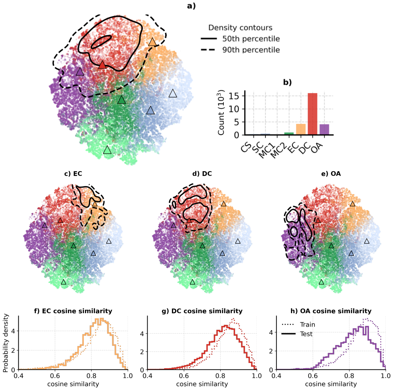
Figure 5.
Physical characterization of the test dataset. (a) Diurnal distribution of test samples for convective classes EC, DC, and OA. (b) Distribution of CC across the three classes. (c–e) Two-dimensional histograms of vs for EC, DC, and OA, respectively, overlaid with training-set density contours (50th, 75th, 90th, 99th percentiles from the innermost to the outermost contour) and mean values (crosses). (f–h) Same as (c–e), but for vs . (c-h) Since COT is available only during daytime conditions, we retained only crops with a timestamp going from 5 to 17 UTC.
Figure 5.
Physical characterization of the test dataset. (a) Diurnal distribution of test samples for convective classes EC, DC, and OA. (b) Distribution of CC across the three classes. (c–e) Two-dimensional histograms of vs for EC, DC, and OA, respectively, overlaid with training-set density contours (50th, 75th, 90th, 99th percentiles from the innermost to the outermost contour) and mean values (crosses). (f–h) Same as (c–e), but for vs . (c-h) Since COT is available only during daytime conditions, we retained only crops with a timestamp going from 5 to 17 UTC.
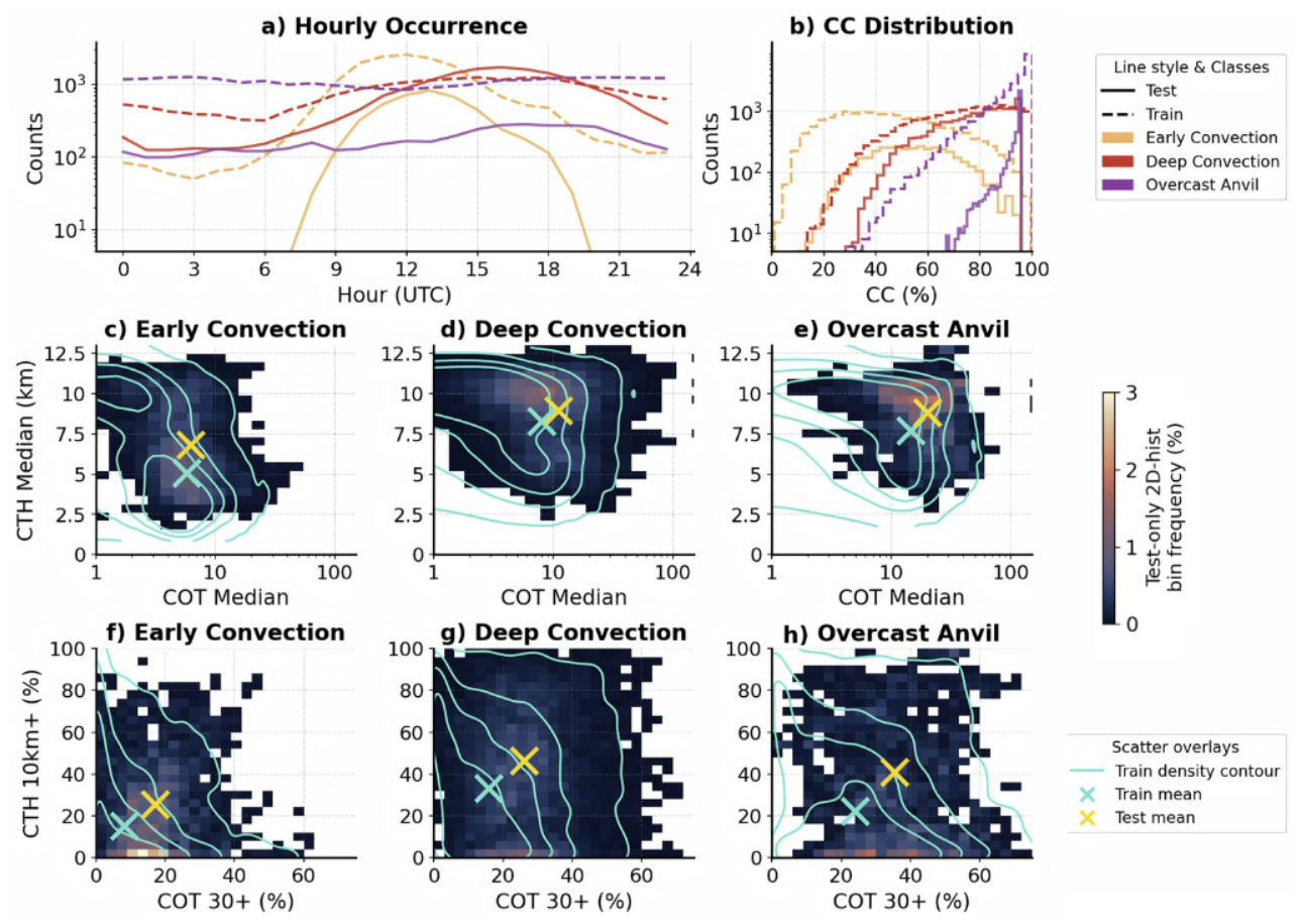
Figure 6.
Randomly selected crops from trajectories associated with EC->DC pathway (a) and DC persistence (b). The frame color around the image crops represents the assigned cloud class color (EC: yellow, DC: red).
Figure 6.
Randomly selected crops from trajectories associated with EC->DC pathway (a) and DC persistence (b). The frame color around the image crops represents the assigned cloud class color (EC: yellow, DC: red).
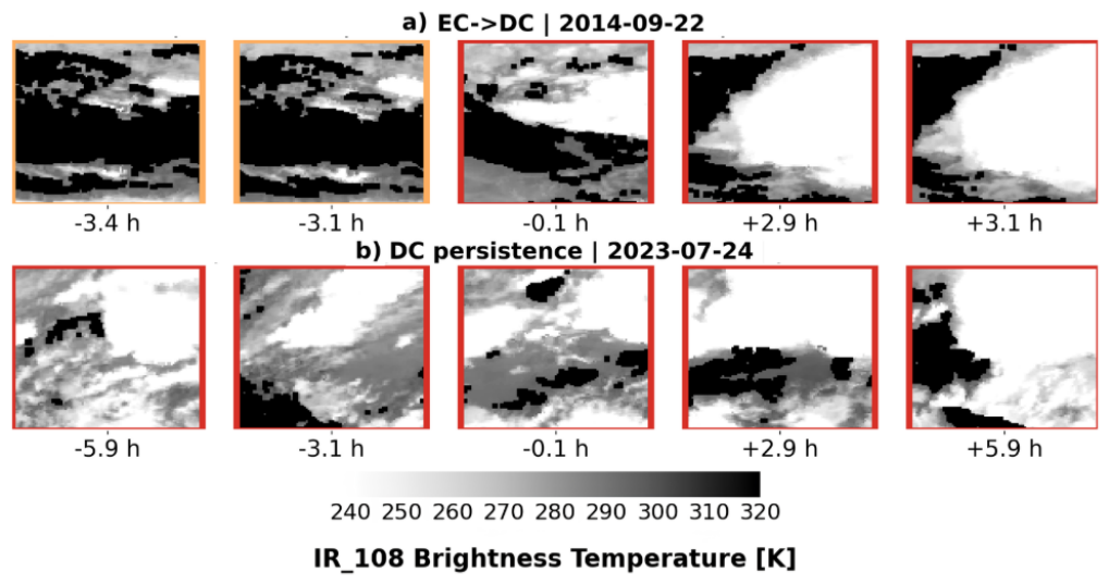
Figure 7.
Hourly-averaged and time-aligned temporal characterization of the two most common pathways: EC→DC (a) and DC persistence (b). From top to bottom: (1a–1b) t-SNE feature-space embedding showing density contours for the full test set together with the trajectories associated with each pathway; (2a–2b) temporal evolution of cosine similarity for the classes characteristic of the pathway, with class-transition counts overlaid on the right-hand axis when two classes are involved; (3a–3b) CTHmedian and COTmedian; (4a–4b) temporal trends of the cloud-area-fraction metrics CTH10+ and COT30+; and (5a–5b) cumulative rainfall trends. (6a–6b) hourly crops count for daytime (5-17 UTC) and nighttime (18-4 UTC). Only hourly bins containing at least 50 crops are shown, and the metrics hourly statistics of COTmedian and COT30+ are computed only if at least 50 daytime crops are available.
Figure 7.
Hourly-averaged and time-aligned temporal characterization of the two most common pathways: EC→DC (a) and DC persistence (b). From top to bottom: (1a–1b) t-SNE feature-space embedding showing density contours for the full test set together with the trajectories associated with each pathway; (2a–2b) temporal evolution of cosine similarity for the classes characteristic of the pathway, with class-transition counts overlaid on the right-hand axis when two classes are involved; (3a–3b) CTHmedian and COTmedian; (4a–4b) temporal trends of the cloud-area-fraction metrics CTH10+ and COT30+; and (5a–5b) cumulative rainfall trends. (6a–6b) hourly crops count for daytime (5-17 UTC) and nighttime (18-4 UTC). Only hourly bins containing at least 50 crops are shown, and the metrics hourly statistics of COTmedian and COT30+ are computed only if at least 50 daytime crops are available.
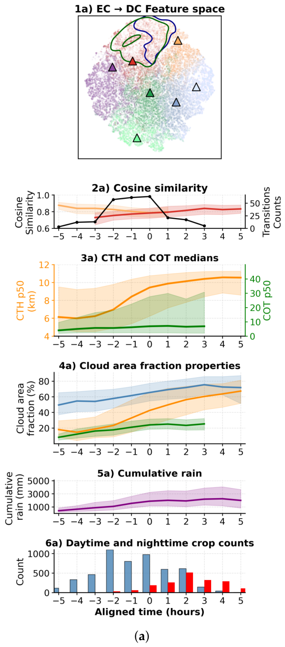
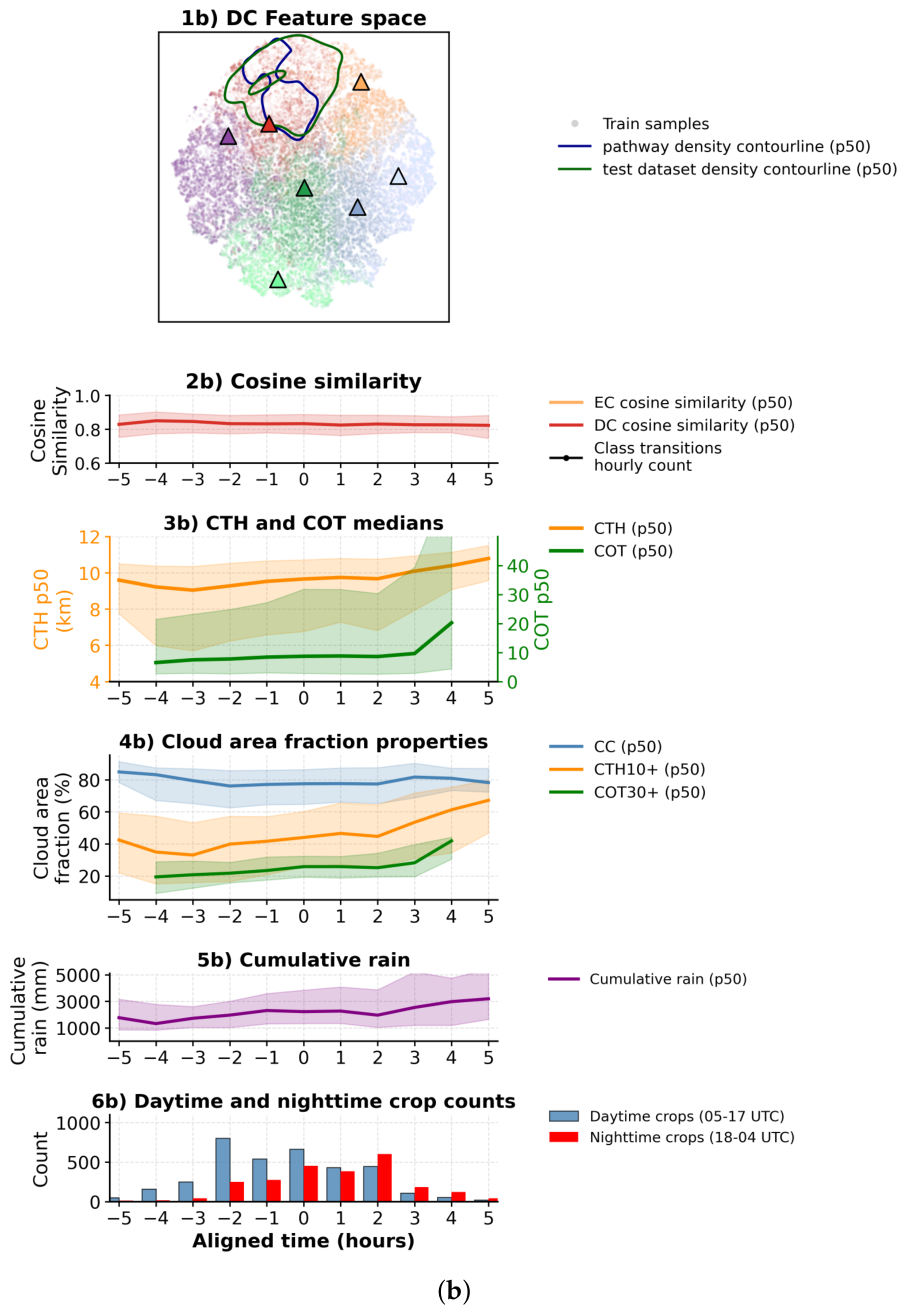

Table 1.
Physical variables used for characterizing cloud regimes computed for every crop.
| Variable | Short name | Range [Units] | Description |
|---|---|---|---|
| Cloud cover | CC | 0–100 [%] | Fraction of pixels classified as cloudy by the cloud mask |
| Median Cloud Top Height | CTHMedian | 0–12 [km] | 50th percentile of CTH distribution |
| Very High Cloud Cover | CTH10+ | 0–100 [%] | Percentage of cloudy pixels with CTH > 10 km |
| Median Cloud Optical Thickness | COTMedian | 0–150 | 50th percentile of COT distribution |
| High Optical Thickness Cover | COT30+ | 0–100 [%] | Percentage of cloudy pixels with COT > 30 |
Table 2.
Pathways ranked by frequency, showing the mean and standard deviation across all trajectories belonging to each pathway for CTHmedian (km) COTmedian CC (%) CTH10+ (%) COT30+ (%). The two most frequent pathways are highlighted in gray.
Table 2.
Pathways ranked by frequency, showing the mean and standard deviation across all trajectories belonging to each pathway for CTHmedian (km) COTmedian CC (%) CTH10+ (%) COT30+ (%). The two most frequent pathways are highlighted in gray.
| Pathway | N storms | CTHmedian (km) | COTmedian | CC (%) | CTH10+ (%) | COT30+ (%) |
|---|---|---|---|---|---|---|
| EC → DC | 253 | 8.73 ± 2.18 | 7.00 ± 4.55 | 63.60 ± 13.42 | 43.32 ± 23.77 | 21.26 ± 7.79 |
| DC | 244 | 8.98 ± 1.96 | 8.94 ± 6.66 | 74.30 ± 13.54 | 41.61 ± 23.19 | 23.87 ± 9.05 |
| DC → OA | 83 | 8.94 ± 1.85 | 14.46 ± 9.30 | 86.54 ± 7.43 | 37.12 ± 27.19 | 30.12 ± 12.44 |
| OA | 55 | 8.69 ± 1.90 | 18.59 ± 10.15 | 93.09 ± 4.52 | 33.63 ± 26.51 | 33.87 ± 13.95 |
| DC → EC → DC | 48 | 8.60 ± 2.35 | 8.07 ± 4.65 | 67.29 ± 11.45 | 39.01 ± 24.93 | 22.34 ± 8.29 |
| EC | 39 | 6.37 ± 2.63 | 5.82 ± 2.32 | 48.72 ± 17.52 | 25.61 ± 25.79 | 16.40 ± 5.80 |
| OA → DC | 33 | 8.55 ± 2.10 | 13.69 ± 7.37 | 88.72 ± 6.47 | 35.35 ± 25.57 | 25.97 ± 11.13 |
| OA → DC → OA | 30 | 9.08 ± 1.82 | 18.60 ± 8.16 | 90.03 ± 7.17 | 36.63 ± 25.96 | 34.27 ± 11.77 |
| DC → OA → DC | 27 | 9.58 ± 1.69 | 11.99 ± 7.51 | 86.78 ± 7.95 | 47.70 ± 21.03 | 27.30 ± 8.59 |
| EC → DC → EC | 17 | 7.62 ± 2.62 | 5.86 ± 2.71 | 56.03 ± 14.46 | 37.64 ± 24.22 | 16.63 ± 6.80 |
| EC → DC → OA | 14 | 9.89 ± 1.99 | 10.73 ± 7.82 | 76.70 ± 6.98 | 53.65 ± 29.85 | 25.88 ± 11.06 |
| DC → EC | 11 | 6.67 ± 1.89 | 9.03 ± 6.78 | 63.05 ± 16.89 | 22.91 ± 13.12 | 18.95 ± 10.07 |
| EC → OA → DC | 10 | 9.97 ± 1.33 | 8.63 ± 5.28 | 81.56 ± 8.27 | 52.36 ± 23.70 | 24.56 ± 8.04 |
Disclaimer/Publisher’s Note: The statements, opinions and data contained in all publications are solely those of the individual author(s) and contributor(s) and not of MDPI and/or the editor(s). MDPI and/or the editor(s) disclaim responsibility for any injury to people or property resulting from any ideas, methods, instructions or products referred to in the content. |
© 2026 by the authors. Licensee MDPI, Basel, Switzerland. This article is an open access article distributed under the terms and conditions of the Creative Commons Attribution (CC BY) license (http://creativecommons.org/licenses/by/4.0/).
Copyright: This open access article is published under a Creative Commons CC BY 4.0 license, which permit the free download, distribution, and reuse, provided that the author and preprint are cited in any reuse.


