
Submitted:
01 August 2026
Posted:
03 August 2026
You are already at the latest version
Abstract
Cancer classification is important in biomedical research because it can support diagnosis, disease stage classification, and treatment planning. A classification method is even more valuable for practical purposes if it is based on noninvasively or less invasively obtained features instead of invasive biopsies. In this study, machine learning algorithms were applied to two biomedical datasets for cancer classification and to examine how the structure of the data affects classifier performance. The first dataset is the Breast Tissue dataset, which represents a low-dimensional classification problem with 106 observations and 9 predictors. The second dataset is an osteosarcoma DNA methylation dataset, which represents a high-dimensional classification problem with about 480,000 CpG features and 15 samples. Logistic Regression, Support Vector Machine, Random Forest, and K-Nearest Neighbors were applied and compared using accuracy, precision, recall, and F1-score. Principal Component Analysis was used to reduce the dimension of the DNA methylation dataset before classification.
The results showed that the machine learning methods performed more reliably in the Breast Tissue dataset. Random Forest and Support Vector Machine had the highest accuracy of 0.7895, while K-Nearest Neighbors had the lowest performance. For the DNA methylation dataset, the model performance was not stable across the different train-test splits. Even after Principal Component Analysis, the results changed depending on how the data were divided and how many principal components were used. This shows that high-dimensional biomedical data with small sample sizes can lead to unstable model performance. Overall, this study shows that machine learning is effective in cancer classification, but the results obtained must be interpreted and adopted carefully, keeping in mind the limitations of such algorithms under certain circumstances, especially when the number of features is much larger than the number of samples.
Keywords:
cancer classification
; machine learning
; breast tissue
; DNA methylation
; osteosarcoma
; high-dimensional data
; principal component analysis
; model performance
1. Introduction
Cancer remains a major global health challenge [1]. This is because of its biological complexity and differences among the types of tissues, the stages of the disease, and other features related to genetics and epigenetics [2]. To enhance diagnosis, outcome prediction, and treatment planning, accurate and reliable cancer classification is essential to improve decision-making in biomedical research [3]. A classification method is even more valuable for practical purposes if it is based on noninvasively or less invasively obtained features instead of invasive biopsies. Data-driven analytical approaches for cancer classification are an important step in that direction.
Machine learning has become a powerful and effective tool for cancer classification. It can learn and identify patterns in biological data. In cancer research, we can use machine learning as a tool to classify tissue types, find the differences between disease stages, and support clinical outcomes [3,4]. These methods learn from the data and use the learned patterns to classify new observations. This implies that the structure of the data contributes heavily to the classifier’s performance, as well as its reliability and stability.
In low-dimensional settings, the number of features is relatively small or not too large compared to the number of observations. In this case, machine learning algorithms may have enough information from the samples to learn the patterns in the data. However, in high-dimensional datasets, such as omics datasets, often the number of features is relatively large compared to the number of samples. This results in the well-known ‘too many features but small sample sizes’ problem. This data structure can lead to unreliable and unstable model estimation and model performance [5,6].
In this paper, the DNA methylation dataset is an example of high-dimensional omics data. DNA methylation is a well-studied epigenetic modification involving the addition of a methyl group to the fifth carbon of cytosine, forming 5-methylcytosine, primarily at CpG sites in DNA without altering the DNA sequence [7].
Abnormal patterns in DNA methylation, including hypomethylation, which refers to reduced methylation levels, and hypermethylation, which refers to increased methylation levels, particularly in CpG-rich regions such as gene promoters, have been associated with cancer development and progression [8].
The nature and structure of the DNA methylation data can make it difficult to analyze, especially when the available sample size is small [9,10,11]. Therefore, Principal Component Analysis, a dimension reduction method, was used to reduce the number of features while retaining the relevant information regarding the directions of maximum variability in the dataset before applying classification models [12,13].
In this study, machine learning algorithms were applied to both the low-dimensional breast tissue dataset and the high-dimensional DNA methylation dataset to evaluate how data structure affects model performance. Logistic Regression, Support Vector Machine, Random Forest, and K-Nearest Neighbors were applied and compared using accuracy, precision, recall, and F1-score. As indicated earlier, Principal Component Analysis was applied to the DNA methylation dataset before classification to reduce the number of features while retaining the information regarding dominant directions of variation in the data.
The goal of this study is to evaluate how machine learning algorithms perform under different data conditions and to examine if the classifier’s performance remains reliable when there are a limited number of samples but many features. The focus is not only on model accuracy but on the stability and the reliability of the model performance across different data structures. This is relevant because, especially in high-dimensional biomedical datasets with small sample sizes, model parameter estimates and performance indicators of learning algorithms tend to become unstable and difficult to generalize.
2. Materials and Methods
2.1. Study Design
This study involves two datasets: The first dataset is the Breast Tissue dataset, which represents the low-dimensional problem because the number of predictors in this dataset is relatively small compared to the number of observations. The second dataset was the DNA methylation dataset from osteosarcoma samples, which represents a high-dimensional scenario because the number of features is much larger than the number of samples.
This study was designed as a comparative machine learning analysis to evaluate model performance in both the low-dimensional and high-dimensional settings.
Logistic Regression, Support Vector Machine, Random Forest, and K-Nearest Neighbors were compared in the low- and high-dimensional scenarios. In the high-dimensional dataset, Principal Component Analysis was applied to reduce the number of features before classification.
2.2. Datasets
Among the two datasets used in this study, the first is the Breast Tissue dataset. It consists of 106 observations and 9 numerical predictor variables. The predictor variables include I0 (impedivity at zero frequency, measured in ohms), PA500 (phase angle at 500 kHz), HFS (high-frequency slope of the phase angle), DA (impedance distance between the spectral ends), Area (area under the impedance spectrum), A/DA (area normalized by DA), Max IP (maximum of the impedance spectrum), DR (distance between I0 and the real part of the maximum-frequency point), and P (length of the spectral curve). The response variable is the breast tissue class, making the dataset a multiclass classification problem. The tissue classes include adi (adipose), car (carcinoma), con (connective), fad (fibro-adenoma), gla (glandular), and mas (mastopathy). Since the number of predictors is small compared to the number of observations, this dataset represents a low-dimensional classification problem.
The second dataset is the DNA methylation dataset from osteosarcoma samples. It contains DNA methylation difference scores (‘diffscore’) measured across CpG sites using the Illumina Infinium HumanMethylation450 platform. Each CpG site is a feature, while each osteosarcoma patient is a sample observation. The methylation difference score represents the difference between methylation levels in tumor samples and the average methylation levels in control samples. Positive values indicate hypermethylation, while negative values indicate hypomethylation. See Appendix A for the details of this ‘diffscore’ computation.
The ‘control’ tissue sample that each of the osteosarcoma patient sample was compared with in order to compute the difference score (‘diffscore’) values is actually an average of six different normal tissue samples — adult skeletal muscle, fetal liver, fetal brain, adult adipose tissue, normal adult bone, normal fetal bone.
Clearly, this DNA methylation dataset poses a high-dimensional classification problem because the number of CpG features is much larger than the number of samples. In this study, the disease stage was used as the response variable, where 0 stands for early stage and 1 for advanced stage. As mentioned earlier, Principal Component Analysis was applied to reduce the number of features before applying the machine learning algorithms.
Table 1 summarizes the main characteristics of the two datasets used in this study.
2.3. Data Preprocessing
Data preprocessing was done to prepare both datasets before applying the machine learning models. For the Breast Tissue dataset, the data was first imported and checked to understand the structure of the variables. The column names were cleaned to make them suitable for analysis in R. R is an open-source programming language and software environment used for statistical computing, graphics, and data analysis. Any case or identification column was removed because it does not add information to the classification problem.
The response variable, which is the breast tissue class, was converted into a factor because the problem is a classification problem. The predictor variables were also converted into a numerical format. The dataset was checked for missing values, and missing values in the predictor variables were replaced using the median value of each variable. In some of the classification models, predictors with near-zero variance were removed because they do not contribute much information to the model.
The Breast Tissue dataset was divided into training and testing datasets using an 80/20 split. The training dataset was used to train models, while the testing dataset was used to evaluate how the models perform on unseen data. A seed value of 42 was used to make the results reproducible. Since the predictor variables were measured on different scales, the variables were standardized by centering and scaling. This was important because models such as Support Vector Machine and K-Nearest Neighbors are affected by differences in the scale of the variables.
For the DNA methylation dataset, the data was first imported together with the supplementary sample information. The dataset was checked for missing values before the analysis. The methylation difference score columns were selected for the analysis because they represent the difference between methylation levels in tumor samples and control samples.
The DNA methylation dataset was originally arranged in a way that CpG sites were rows and samples were columns. Since machine learning models require observations as rows and features as columns, the dataset was transposed so that the osteosarcoma samples became the rows and the CpG sites became columns. Constant or almost zero-variance CpG features were removed because they do not provide useful variation for the analysis.
The methylation data was standardized before applying Principal Component Analysis. Principal Component Analysis was then used to reduce the very large number of features into a smaller number of principal components while retaining the dominant directions of variation in the data. The first eight principal components were retained and used as the predictor variables for classification. The Stage variable was added as the response variable, where 0 represents early stage and 1 represents advanced stage.
After preprocessing, Logistic Regression, Support Vector Machine, Random Forest, and K-Nearest Neighbors were applied to the datasets. For the DNA methylation dataset, different train-test splits were also used to examine how stable the model’s performance was under different data partitions.
2.4. Principal Component Analysis
Principal Component Analysis was applied to the DNA methylation dataset because the dataset is high-dimensional. The number of CpG features was much larger than the number of samples, and this can make the machine learning models unstable. Principal Component Analysis is a dimension reduction method that combines the original variables into a smaller number of mutually perpendicular linear combinations called principal components. These principal components retain most of the variation in the original data [12,13].
The data was also standardized before the analysis so that the features can contribute equally to the principal components. The principal components were selected based on the proportion of variance explained by them and the cumulative variance proportion they explain together. In this study, the first eight principal components were retained because they explained approximately 81.6% of the total variance in the DNA methylation dataset. These eight principal components were used as the predictor variables for the machine learning models. This significant reduction facilitated the implementation of Logistic Regression, Support Vector Machine, Random Forest, and K-Nearest Neighbors to this dataset for disease stage classification.
2.5. Machine Learning Models
The four classifiers Logistic Regression, Support Vector Machine, Random Forest, and K-Nearest Neighbors were selected because they are commonly used for classification problems and represent different ways of learning patterns from data [13,14].
Logistic Regression estimates the relationship between predictor variables and a categorical outcome by modeling the log-odds of class membership as a linear combination of the predictors. The logistic function transforms this linear predictor into a probability between 0 and 1. In binary classification, the predicted probability is compared with a classification threshold to assign an observation to one of two classes. Multinomial Logistic Regression extends the same principle to outcomes with more than two categories by estimating the log-odds of each category relative to a reference category [13,15]. In the Breast Tissue dataset, multinomial Logistic Regression was applied because the response variable had six tissue classes. In the DNA methylation dataset, binary Logistic Regression was used because disease stage was coded as 0 for early stage and 1 for advanced stage.
Support Vector Machine constructs a decision boundary, called a hyperplane, that separates the classes while maximizing the margin between the boundary and the nearest training observations from each class. These nearest observations are called support vectors because they largely determine the position of the decision boundary. When the classes cannot be separated adequately by a straight boundary, a kernel function can represent the data in a higher-dimensional feature space where separation may be easier. Common kernels include linear, radial basis function, polynomial, and sigmoid kernels. The regularization parameter controls the balance between obtaining a wider margin and allowing classification errors [16,17]. For the Breast Tissue dataset, linear, radial, polynomial, and sigmoid kernels were considered. For the DNA methylation dataset, a linear Support Vector Machine was applied using the retained principal components as predictors.
Random Forest is an ensemble method that builds many decision trees rather than relying on a single tree. Each tree is trained using a bootstrap sample drawn from the training data, and only a randomly selected subset of predictors is considered at each possible split. This additional randomization reduces correlation among the trees. Each tree recursively divides the predictor space into increasingly homogeneous groups, and the final class is determined by majority voting across the trees. Combining many partly independent trees usually reduces prediction variance and makes the model less sensitive to the instability of an individual decision tree. Random Forest can also capture nonlinear relationships and interactions among predictors and can provide measures of predictor importance [18,19]. In this study, Random Forest was applied to both the Breast Tissue dataset and the DNA methylation dataset.
K-Nearest Neighbors is a nonparametric, instance-based method that does not estimate an explicit mathematical model during training. To classify a new observation, the algorithm calculates its distance from the observations in the training dataset, identifies the K closest observations, and assigns the class most common among those neighbors. The choice of K affects the flexibility of the classifier: a small value can make the model sensitive to noise and individual observations, whereas a larger value produces a smoother decision boundary but may overlook local class structure. Because the method is based on distances, predictor scaling is important, and its performance can deteriorate when irrelevant variables or very high-dimensional feature spaces make distances less informative [20]. The predictor variables were therefore standardized before K-Nearest Neighbors was applied.
For the Breast Tissue dataset, the models were applied directly after preprocessing because the dataset was low-dimensional. For the DNA methylation dataset, the models were applied after Principal Component Analysis because the original number of CpG features was much larger than the number of samples. The same set of models was used so that their performance could be compared under low-dimensional and high-dimensional data conditions.
2.6. Model Evaluation
The performance of the machine learning models was evaluated using accuracy, precision, recall, and F1-score. These metrics were used to compare how well each model classified the observations in both the low-dimensional and high-dimensional datasets.
Accuracy was used to measure the overall proportion of correctly classified observations. Precision was used to measure how many of the predicted class labels were correctly classified. Recall was used to measure how many of the actual class observations were correctly identified by the model. The F1-score was also used because it gives a balance between precision and recall.
For the Breast Tissue dataset, the data were divided into training and testing datasets using an 80/20 split. The training dataset was used to train the models, while the testing dataset was used to evaluate model performance on unseen data.
For the DNA methylation dataset, model evaluation was done using different train-test splits because the sample size was small. The splits used were 80/20, 70/30, and 60/40. This was done to examine whether the model performance remained stable when the data partition changed. This was important because in a high-dimensional dataset with small sample size, model performance can change depending on which samples are included in the training and testing datasets.
The evaluation was therefore based not only on the performance values, but also on how stable the models were across different data conditions.
3. Results
3.1. Breast Tissue Classification Results
Figure 1 shows the 3D PCA plot of the Breast Tissue dataset using the first three principal components. The plot was used to visualize the structure of the dataset and to see how the tissue classes are distributed in the reduced feature space. From the plot, some tissue classes show visible separation, while some classes overlap. This means that some classes may be easier for the machine learning models to classify, while overlapping classes may be more difficult to classify correctly.
Principal Component Analysis was used here only for visualization of the Breast Tissue dataset. The machine learning models for the Breast Tissue dataset were trained using the original predictor variables after preprocessing. On the other hand, as has been pointed out earlier, PCA was used as a dimension reduction step for the DNA methylation dataset because the number of CpG features was much larger than the number of samples.
Table 2 presents the comparative performance of the machine learning models applied to the Breast Tissue dataset. Random Forest and SVM with linear kernel achieved the highest accuracy of 0.7895. The SVM linear model also recorded the highest precision of 0.8056 and the highest F1-score of 0.7841, showing strong overall classification performance. Random Forest had the highest recall of 0.7917, indicating that it identified more of the actual class observations correctly. Logistic Regression showed moderate performance, while K-NN with k = 5 had the lowest performance across all the evaluation metrics.
3.2. DNA Methylation Principal Component Analysis (PCA) Results
Table 3 shows the variance explained by the principal components from the DNA methylation dataset. In this study, the first eight principal components were used for the main machine learning analysis because they retained more than 80% of the total variation in the data. This reduced the large number of DNA methylation features into a smaller number of linear combinations while still retaining the dominant directions of variation in the dataset. Additional analyses using fewer and more principal components were also considered to examine how the number of retained components affected model performance.
Although PC1 to PC14 together explained all the variation in the dataset, all the components were not used for the main classification analysis because the number of samples was small. Using too many principal components with a small sample size may increase model instability and reduce the reliability of the performance estimates.
Figure 2 shows the scree plot of the principal components from the DNA methylation dataset. The plot shows that the first few principal components explained more variation than the later components. The curve decreases gradually as the number of principal components increases. This means that the variation in the DNA methylation dataset was spread across several principal components.
The scree plot supports the use of the first eight principal components for the main machine learning analysis because PC1 to PC8 explained about 81.60% of the total variation in the data. After the eighth principal component, the additional components contributed smaller amounts of variation.
3.3. DNA Methylation Classification Results
So, the first eight principal components were used as the predictor variables for disease stage classification. Logistic Regression, Support Vector Machine, Random Forest, and K-Nearest Neighbors were applied to the DNA methylation dataset using PC1 to PC8. Since the sample size was small, different train-test splits were used to check how the model performance changes.
Table 4 shows the model performance across the 80/20, 70/30, and 60/40 train-test splits. From the table, the model performance changes across different splits. In the 80/20 split, all the models had the same accuracy of 0.3333 and F1-score of 0.5000. In the 70/30 split, Logistic Regression had the highest performance with accuracy, precision, recall, and F1-score all equal to 1.0000, while the other models performed lower. In the 60/40 split, Logistic Regression also performed better than the other models, but the performance was not the same as the 70/30 split.
This shows that the model performance in the DNA methylation dataset was not stable across the different train-test splits. The results suggest that the small sample size affected the reliability of the machine learning models, even after Principal Component Analysis was used to reduce the dimension of the data.
3.4. Sensitivity Analysis Using Different Numbers of Principal Components
Table 5 shows the sensitivity analysis using different numbers of principal components. The results show that when the number of principal components changed, the model performance also changed. When PC1 to PC5 were used, the model performance changed across the train-test splits, and some models had zero precision, recall, and F1-score. When PC1 to PC8 were used, Logistic Regression gave high performance in some splits, but the overall result still showed instability. When PC1 to PC11 were used, more variation was retained in the data, but the model performance was still unstable across the splits.
This shows that increasing the number of principal components did not automatically improve the model performance. The result also shows that the DNA methylation classification was sensitive to the number of principal components used and how the data was divided into training and testing datasets.
3.5. Summary of Results
Overall, the results show that the machine learning models performed differently in the Breast Tissue dataset and the DNA methylation dataset. In the Breast Tissue dataset, Random Forest and Support Vector Machine performed better than the other models. Logistic Regression showed moderate performance, while K-Nearest Neighbors had the lowest performance.
In the DNA methylation dataset, the model performance was not stable across the different train-test splits. Even though Principal Component Analysis was used to reduce the dimension of the data, the performance still changed depending on how the data was divided into training and testing datasets.
The sensitivity analysis also showed that when the number of principal components changed, the model performance also changed. This means that the DNA methylation classification was affected by both the number of principal components used and the train-test split. These results show that the machine learning models performed more reliably in the low-dimensional Breast Tissue dataset than in the high-dimensional DNA methylation dataset with small sample size.
4. Discussion
4.1. Interpretation of Breast Tissue Results
The Breast Tissue dataset was the low-dimensional dataset used in this study. The number of predictors was small compared to the number of observations, and this made it easier for the machine learning models to learn the pattern in the data. From the results, Random Forest and Support Vector Machine performed better than Logistic Regression and K-Nearest Neighbors.
Random Forest performed well because it can learn complex patterns in the data. It combines many decision trees, and this helps the model to improve classification performance. This may be why Random Forest had high accuracy and recall in the Breast Tissue dataset.
Support Vector Machine with the linear kernel also performed well. This shows that some of the tissue classes were separated well using the predictor variables. The SVM model had the highest precision and F1-score, which means it performed well in classifying the tissue classes.
Logistic Regression showed moderate performance. This may be because Logistic Regression uses a linear decision boundary, and this may not fully capture the pattern among all the tissue classes. However, it still performed better than K-Nearest Neighbors.
K-Nearest Neighbors had the lowest performance. This may be because K-Nearest Neighbors depends on distance between observations. If some tissue classes overlap or have similar values, the model may find it difficult to classify them correctly. This may explain why K-Nearest Neighbors did not perform as well as Random Forest and Support Vector Machine.
Overall, the Breast Tissue results show that the models performed better in the low-dimensional dataset. The results also show that the choice of model is important because the models did not perform the same on the same dataset.
4.2. Interpretation of DNA Methylation Results
The DNA methylation dataset was the high-dimensional dataset used in this study. The number of CpG features was much larger than the number of samples, and this made the analysis more difficult. Even though Principal Component Analysis was used to reduce the dimension of the data, the model performance was still not stable across the different train-test splits.
From the results, the models did not perform the same when the train-test split changed. In the 80/20 split, all the models had low performance. In the 70/30 split, Logistic Regression gave very high performance, but this result should be interpreted carefully because the sample size was small. In the 60/40 split, Logistic Regression still performed better than the other models, but the performance was not the same as the 70/30 split.
This shows that the DNA methylation results were affected by how the data was divided into training and testing datasets. Since the sample size was small, changing the samples in the training and testing sets changed the model performance. This means that the high performance in some splits may not represent true model reliability.
Random Forest, Support Vector Machine, and K-Nearest Neighbors did not show consistent performance across the splits. This may be because the number of samples was too small for the models to learn stable patterns from the data. The high-dimensional structure of the DNA methylation data also made the classification problem more difficult.
Overall, the DNA methylation results show that machine learning performance can become unstable when the dataset has many features but only few samples. This means that the results from high-dimensional biomedical data should be interpreted carefully, especially when the sample size is limited.
4.3. Implications of the Study
The results of this study show that the structure of the data is important when applying machine learning models for cancer classification. In the Breast Tissue dataset, the models performed better because the number of predictors was small compared to the number of observations. This means that when the dataset has enough observations compared to the number of features, the models may learn the pattern in the data better.
For the DNA methylation dataset, the results showed that high-dimensional data with small sample size can make model performance unstable. Even after Principal Component Analysis was used to reduce the dimension of the data, the performance still changed across the train-test splits. The performance also changed when the number of principal components changed. This shows that high accuracy in one split does not always mean that the model is reliable.
This is important in cancer classification because machine learning models can support diagnosis, disease stage classification, and treatment planning. If the model’s performance is not stable, then the result may be difficult to trust for decision-making. This is more important in omics data, where the number of features is very large and the number of samples may be small.
The study also shows that model evaluation should not depend only on accuracy. Precision, recall, F1-score, and stability across different splits should also be considered. This helps to know if the model is learning useful patterns or if the result is affected by the small sample size and how the data was divided.
Overall, this study shows that machine learning can support cancer classification, but the results must be interpreted carefully. For high-dimensional biomedical data, enough sample size, proper validation, and careful feature reduction are important to improve the reliability of model performance.
4.4. Limitations
This study has some limitations. The first limitation is the small sample size, especially in the DNA methylation dataset. The DNA methylation dataset had about 480,000 CpG features but only 15 samples. Because of this, the number of features was much larger than the number of samples, and this made it difficult for the machine learning models to learn stable patterns from the data.
Another limitation is that the model performance was evaluated using train-test splits. Even though different train-test splits were used, the small sample size still made the results sensitive to how the data was divided. This means that some high-performance values may be due to the specific samples in the training and testing datasets.
Also, Principal Component Analysis was used to reduce the dimension of the DNA methylation data. Even though PCA helped to reduce the number of features, it may also remove some information from the original data. The number of principal components used also affected the model performance, which shows that the results can change depending on the dimension reduction choice.
Another limitation is that external validation was not used. The models were tested only on the available datasets. Without an independent external dataset, it is difficult to confirm whether the models will perform the same way on new biomedical data.
Overall, these limitations show that the results should be interpreted carefully, especially for the DNA methylation dataset. Future studies should use larger sample sizes, external validation datasets, and more robust validation methods to improve the reliability of model performance.
5. Conclusions
This study compared machine learning performance in a low-dimensional Breast Tissue dataset and a high-dimensional DNA methylation dataset. Logistic Regression, Support Vector Machine, Random Forest, and K-Nearest Neighbors were applied to both datasets to examine how the structure of the data affects model performance.
The results showed that the models performed more reliably in the Breast Tissue dataset. Random Forest and Support Vector Machine had the highest performance in the main analysis, while Logistic Regression showed moderate performance and K-Nearest Neighbors had the lowest performance. This shows that machine learning models can perform better when the number of predictors is small compared to the number of observations.
For the DNA methylation dataset, the results were not stable across the different train-test splits. The dataset had about 480,000 CpG features but only 15 samples, which made the classification problem more difficult. Even after Principal Component Analysis was used to reduce the dimension of the data, the model performance still changed across the splits and across the number of principal components used.
Overall, this study shows that machine learning can support cancer classification, but the reliability of the results depends on the structure of the data. In high-dimensional biomedical data with small sample size, high performance in one split should be interpreted carefully. Future studies should use larger sample sizes, external validation datasets, and stronger validation methods to improve the reliability of machine learning models in cancer classification.
Author Contributions
Conceptualization, E.K.A. and S.D.; methodology, E.K.A. and S.D.; software, E.K.A.; formal analysis, E.K.A.; investigation, E.K.A.; data curation, E.K.A.; writing—original draft preparation, E.K.A.; writing—review and editing, E.K.A. and S.D.; supervision, S.D. All authors have read and agreed to the published version of the manuscript.
Funding
This research received no external funding.
Institutional Review Board Statement
Not applicable. This study used publicly available and/or previously collected anonymized datasets and did not involve new human-subject recruitment or intervention.
Informed Consent Statement
Not applicable. This study used publicly available and/or previously collected anonymized datasets, and no new human participants were recruited for this research.
Data Availability Statement
The Breast Tissue dataset analyzed in this study is publicly available from the UCI Machine Learning Repository at https://doi.org/10.24432/C5P31H. The osteosarcoma DNA methylation dataset was obtained from the Division of Hematology/Oncology, Department of Pediatrics, Akron Children’s Hospital, Akron, Ohio, USA. The dataset contains de-identified patient data and is available from Dr. Sujay Datta upon reasonable request. Requests for access should be directed to Dr. Sujay Datta.
Conflicts of Interest
The authors declare no conflicts of interest.
Acknowledgments
This article was developed from a master’s paper completed in the Department of Statistics at The University of Akron. The authors thank the Department of Statistics at The University of Akron for the academic support provided during the development of this work.
Appendix A. Computation of DNA Methylation DiffScores
Computation of the beta values
The beta value (β) estimates the methylation level of a CpG locus from the relative intensities of the methylated and unmethylated alleles. For the Infinium Methylation Assay, β was calculated as:
β = max(Signal B, 0) / [max(Signal A, 0) + max(Signal B, 0) + 100]
For Infinium I assays, signals A and B are produced by two different bead types and reported in the same color. For Infinium II assays, which were used in this project, signal A is the red-channel signal representing the unmethylated allele, while signal B is the green-channel signal representing the methylated allele.
Differential methylation analysis algorithms
The differential methylation analysis compares a condition group with a reference group. GenomeStudio provides three error models for this comparison: (1) the Illumina Custom Model, (2) the Mann–Whitney Model, and (3) the t-Test Model.
(1) Illumina Custom Model
The Illumina Custom Model assumes that the methylation beta value is normally distributed among replicates corresponding to a set of biological conditions. The variation in the estimate of β is treated as a function of β. This function was estimated by repeatedly measuring loci with known methylation fractions from 0 to 1 and fitting a parabola to the standard deviation as a function of β:
s = Aβ2 + Bβ + C
For GoldenGate and Infinium Methylation assays, A = −0.1511, B = 0.1444, and C = 0.01646. For VeraCode Methylation, A = −0.1582, B = 0.1554, and C = 0.00756. The two-sided p-value for each interrogated site is then calculated as:
p = z{|βcond − βref| / √[(scond2/Ncond) + (sref2/Nref)]}
Here, z(x) denotes the two-sided tail area beyond the value x under the standard normal curve.
(2) Mann–Whitney Model
The Mann–Whitney test generates an exact two-sided p-value from the Mann–Whitney U distribution when either sample size is less than 3 or when the larger sample size is less than 22. Otherwise, the normal approximation is used. Observations from the condition and reference samples are combined and ranked from smallest to largest. Tied observations receive their average rank. The test statistic is the total rank of the observations in one group. For small samples, this statistic is compared with the Mann–Whitney U distribution. For larger samples, the statistic is standardized and its absolute value is compared with the standard normal distribution to obtain the approximate two-sided p-value. When ties are present, an adjusted standard deviation is used during standardization.
(3) t-Test Model
When either the reference group or the condition group contains at least two replicate samples, variance is estimated across the replicate samples. Otherwise, variance is estimated from bead-to-bead variation. This method uses the pooled two-sample t-test and assumes equal variances for the two groups.
The Illumina Custom Model and the t-Test Model are based on a normality assumption for the methylation beta values, whereas the Mann–Whitney Model is not. When the normality assumption is violated, the Mann–Whitney Model is more appropriate. When normality is reasonable and the reference and condition groups have equal variances, the t-Test Model is appropriate. For large samples, the Illumina Custom Model may be preferred. GenomeStudio does not provide a Welch–Satterthwaite unequal-variance t-test option.
Conversion of p-values to DiffScores
After a p-value is obtained using one of the models above, it is converted to a DiffScore to make comparisons easier. The DiffScore is calculated as:
DiffScore = sgn(βcond − βref) × 10 × |log10(p)|
Equivalently, p = 10^(−|DiffScore|/10). The function sgn(x) gives the sign of the difference between the condition and reference beta values. A positive DiffScore indicates higher methylation in the condition group, while a negative DiffScore indicates lower methylation. For example, p-values of 0.05, 0.01, and 0.001 correspond approximately to absolute DiffScores of 13, 20, and 30, respectively.
References
- World Health Organization. Cancer. 3 July 2026. Available online: https://www.who.int/news-room/fact-sheets/detail/cancer.
- MacDonald, W. J.; Purcell, C.; Pinho-Schwermann, M.; Stubbs, N. M.; Srinivasan, P. R.; El-Deiry, W. S. Heterogeneity in cancer. Cancers 2025, 17(3), 441. [Google Scholar] [CrossRef] [PubMed]
- Zhang, B.; Shi, H.; Wang, H. Machine learning and AI in cancer prognosis, prediction, and treatment selection: A critical approach. J. Multidiscip. Healthc. 2023, 16, 1779–1791. [Google Scholar] [CrossRef] [PubMed]
- Wang, M.; Chang, W.; Zhang, Y. Artificial intelligence for the diagnosis and management of cancers: Potentials and challenges. MedComm 2025, 6(11), e70460. [Google Scholar] [CrossRef] [PubMed]
- Labory, J.; Njomgue-Fotso, E.; Bottini, S. Benchmarking feature selection and feature extraction methods to improve the performances of machine-learning algorithms for patient classification using metabolomics biomedical data. Comput. Struct. Biotechnol. J. 2024, 23, 1274–1287. [Google Scholar] [CrossRef] [PubMed]
- Torres-Martos, Á.; Bustos-Aibar, M.; Ramírez-Mena, A.; Cámara-Sánchez, S.; Anguita-Ruiz, A.; Alcalá, R.; Aguilera, C. M.; Alcalá-Fdez, J. Omics data preprocessing for machine learning: A case study in childhood obesity. Genes 2023, 14(2), 248. [Google Scholar] [CrossRef] [PubMed]
- Geissler, F.; Nesic, K.; Kondrashova, O.; Dobrovic, A.; Swisher, E. M.; Scott, C. L.; Wakefield, M. J. The role of aberrant DNA methylation in cancer initiation and clinical impacts. Ther. Adv. Med. Oncol. 2024, 16, 17588359231220511. [Google Scholar] [CrossRef] [PubMed]
- Ehrlich, M. DNA hypomethylation in cancer cells. Epigenomics 2009, 1(2), 239–259. [Google Scholar] [CrossRef] [PubMed]
- Model, F.; Adorján, P.; Olek, A.; Piepenbrock, C. Feature selection for DNA methylation based cancer classification. Bioinformatics 2001, 17 (Suppl. 1), S157–S164. [Google Scholar] [CrossRef] [PubMed]
- Yuan, T.; Edelmann, D.; Fan, Z.; Alwers, E.; Kather, J. N.; Brenner, H.; Hoffmeister, M. Machine learning in the identification of prognostic DNA methylation biomarkers among patients with cancer: A systematic review of epigenome-wide studies. Artif. Intell. Med. 2023, 143, 102589. [Google Scholar] [CrossRef] [PubMed]
- Doherty, T.; Dempster, E.; Hannon, E.; Mill, J.; Poulton, R.; Corcoran, D.; Sugden, K.; Williams, B.; Caspi, A.; Moffitt, T. E.; Delany, S. J.; Murphy, T. M. A comparison of feature selection methodologies and learning algorithms in the development of a DNA methylation-based telomere length estimator. BMC Bioinform. 2023, 24, 178. [Google Scholar] [CrossRef] [PubMed]
- Jolliffe, I. T. Principal component analysis, 2nd ed.; Springer, 2002. [Google Scholar] [CrossRef]
- James, G.; Witten, D.; Hastie, T.; Tibshirani, R. An introduction to statistical learning: With applications in R; Springer, 2013. [Google Scholar] [CrossRef]
- Alpaydın, E. Introduction to machine learning, 2nd ed.; MIT Press, 2009. [Google Scholar]
- Schober, P.; Vetter, T. R. Logistic regression in medical research. Anesth. Analg. 2021, 132(2), 365–366. [Google Scholar] [CrossRef] [PubMed]
- Cortes, C.; Vapnik, V. Support-vector networks. Mach. Learn. 1995, 20, 273–297. [Google Scholar] [CrossRef]
- Guido, R.; Ferrisi, S.; Lofaro, D.; Conforti, D. An overview on the advancements of support vector machine models in healthcare applications: A review. Information 2024, 15(4), 235. [Google Scholar] [CrossRef]
- Breiman, L. Random forests. Mach. Learn. 2001, 45, 5–32. [Google Scholar] [CrossRef]
- Hu, J.; Szymczak, S. A review on longitudinal data analysis with random forest. Brief. Bioinform. 2023, 24(2), bbad002. [Google Scholar] [CrossRef] [PubMed]
- Halder, R. K.; Uddin, M. N.; Uddin, M. A.; Aryal, S.; Khraisat, A. Enhancing K-nearest neighbor algorithm: A comprehensive review and performance analysis of modifications. J. Big Data 2024, 11, 113. [Google Scholar] [CrossRef]
- S, J.; Jossinet, J. Breast Tissue [Data set]. In UCI Machine Learning Repository; 1996. [Google Scholar] [CrossRef]
- Jossinet, J. Variability of impedivity in normal and pathological breast tissue. Med. Biol. Eng. Comput. 1996, 34(5), 346–350. [Google Scholar] [CrossRef] [PubMed]
- Estrela da Silva, J.; Marques de Sá, J. P.; Jossinet, J. Classification of breast tissue by electrical impedance spectroscopy. Med. Biol. Eng. Comput. 2000, 38, 26–30. [Google Scholar] [CrossRef] [PubMed]
Figure 1.
3D PCA plot of the Breast Tissue dataset showing the distribution of tissue classes using the first three principal components.
Figure 1.
3D PCA plot of the Breast Tissue dataset showing the distribution of tissue classes using the first three principal components.
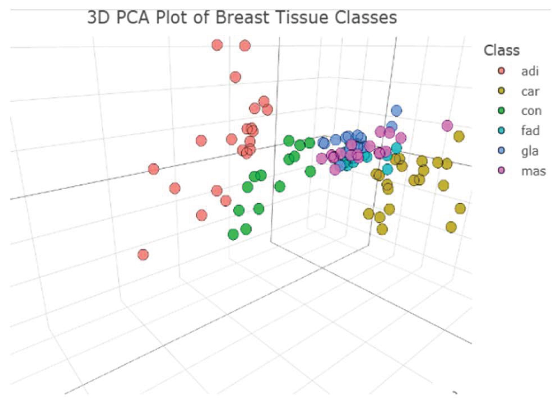
Figure 2.
Scree plot of principal components for the DNA methylation dataset.
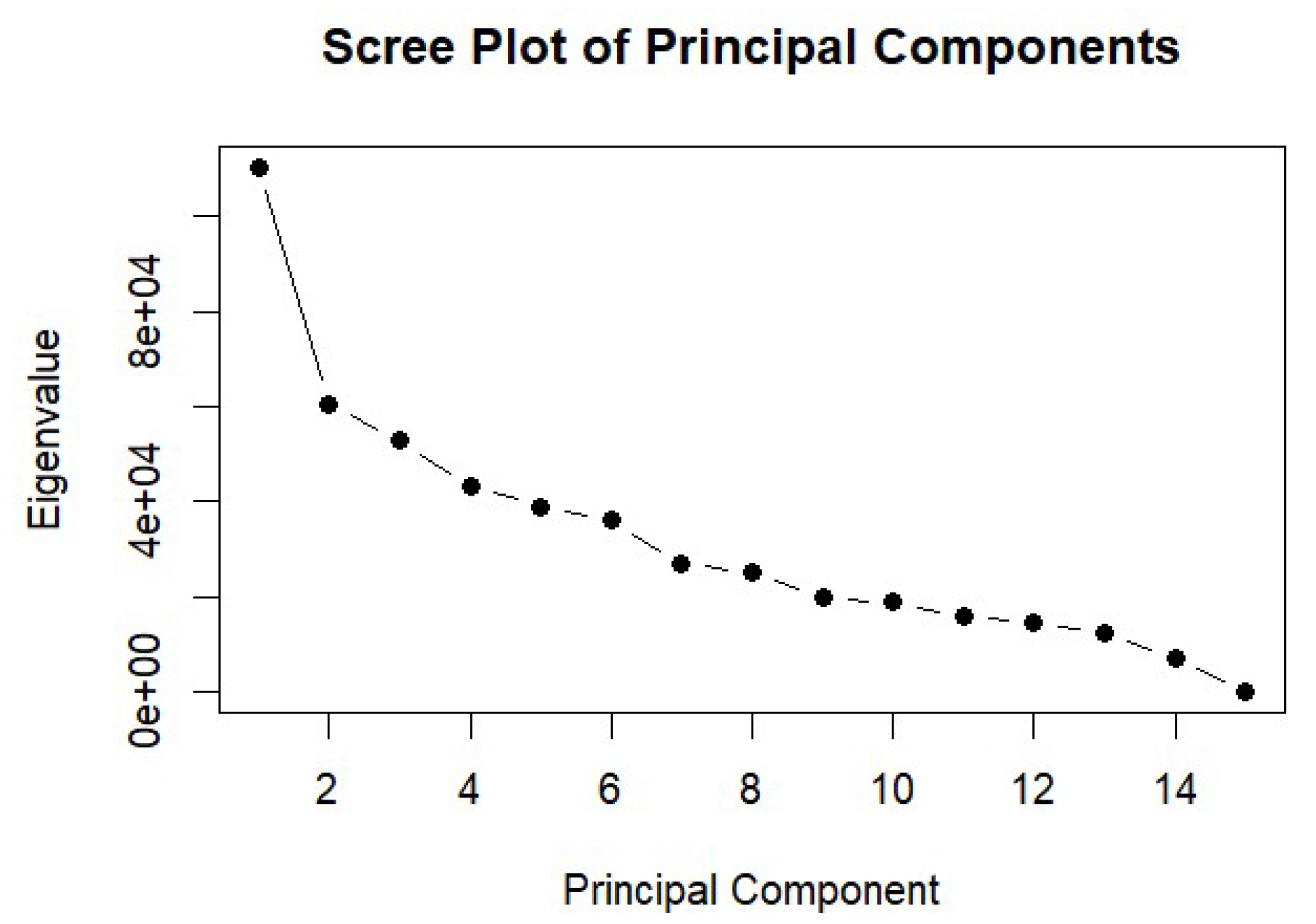

Table 1.
Summary of Datasets used in this study.
| Datasets | Data Type | Sample Size | Number of Features | Response Variable | Classification Type |
|---|---|---|---|---|---|
| Breast Tissue dataset | Numerical data | 106 observations | 9 predictors | Tissue class | Multiclass classification |
| DNA methylation dataset | Osteosarcoma DNA methylation data | 15 samples | CpG features | Disease stage | Binary classification |
Table 2.
Comparative Performance of Machine Learning Models.
| Model | Accuracy | Precision | Recall | F1-score |
|---|---|---|---|---|
| Logistic Regression | 0.6842 | 0.7381 | 0.6944 | 0.6857 |
| Random Forest | 0.7895 | 0.7722 | 0.7917 | 0.7688 |
| SVM (Linear) | 0.7895 | 0.8056 | 0.7778 | 0.7841 |
| K-NN (k = 5) | 0.5789 | 0.5333 | 0.5139 | 0.5230 |
Table 3.
Variance Explained by Principal Components.
| Principal Component | Standard Deviation | Proportion of Variance | Cumulative Variance |
|---|---|---|---|
| PC1 | 332.0698 | 0.2284 | 0.2284 |
| PC2 | 246.0626 | 0.1254 | 0.3538 |
| PC3 | 229.9482 | 0.1095 | 0.4634 |
| PC4 | 207.6440 | 0.0893 | 0.5527 |
| PC5 | 197.5008 | 0.0808 | 0.6335 |
| PC6 | 189.7966 | 0.0746 | 0.7081 |
| PC7 | 164.2466 | 0.0559 | 0.7640 |
| PC8 | 158.5792 | 0.0521 | 0.8160 |
| PC9 | 140.9844 | 0.0412 | 0.8572 |
| PC10 | 137.2794 | 0.0390 | 0.8962 |
| PC11 | 125.9183 | 0.0328 | 0.9291 |
| PC12 | 120.1523 | 0.0299 | 0.9590 |
| PC13 | 111.7906 | 0.0259 | 0.9849 |
| PC14 | 85.4265 | 0.0151 | 1.0000 |
Table 4.
Model Performance Across Different Train-Test Splits.
| Model | Split | Accuracy | Precision | Recall | F1-score |
|---|---|---|---|---|---|
| Logistic Regression | 80/20 | 0.3333 | 0.5000 | 0.5000 | 0.5000 |
| Logistic Regression | 70/30 | 1.0000 | 1.0000 | 1.0000 | 1.0000 |
| Logistic Regression | 60/40 | 0.8333 | 1.0000 | 0.7500 | 0.8571 |
| SVM (Linear) | 80/20 | 0.3333 | 0.5000 | 0.5000 | 0.5000 |
| SVM (Linear) | 70/30 | 0.4000 | 0.5000 | 0.3333 | 0.4000 |
| SVM (Linear) | 60/40 | 0.3333 | 0.5000 | 0.5000 | 0.5000 |
| Random Forest | 80/20 | 0.3333 | 0.5000 | 0.5000 | 0.5000 |
| Random Forest | 70/30 | 0.4000 | 0.5000 | 0.3333 | 0.4000 |
| Random Forest | 60/40 | 0.5000 | 0.6667 | 0.5000 | 0.5714 |
| KNN (k = 3) | 80/20 | 0.3333 | 0.5000 | 0.5000 | 0.5000 |
| KNN (k = 3) | 70/30 | 0.4000 | 0.5000 | 0.3333 | 0.4000 |
| KNN (k = 3) | 60/40 | 0.5000 | 0.6667 | 0.5000 | 0.5714 |
Table 5.
Sensitivity Analysis Using Different Numbers of Principal Components.
| PC Features Used | Cumulative Variance | Observation |
|---|---|---|
| PC1 – PC5 | 63.35% | Performance changed across the train-test splits, and some models produced zero precision, recall, and F1-score. |
| PC1 – PC8 | 81.60% | Logistic Regression gave high performance in some splits, but the overall results still showed instability. |
| PC1 – PC11 | 92.91% | More variation retained but performance was still unstable |
Disclaimer/Publisher’s Note: The statements, opinions and data contained in all publications are solely those of the individual author(s) and contributor(s) and not of MDPI and/or the editor(s). MDPI and/or the editor(s) disclaim responsibility for any injury to people or property resulting from any ideas, methods, instructions or products referred to in the content. |
© 2026 by the authors. Licensee MDPI, Basel, Switzerland. This article is an open access article distributed under the terms and conditions of the Creative Commons Attribution (CC BY) license (http://creativecommons.org/licenses/by/4.0/).
Copyright: This open access article is published under a Creative Commons CC BY 4.0 license, which permit the free download, distribution, and reuse, provided that the author and preprint are cited in any reuse.


