

Submitted:
01 August 2026
Posted:
03 August 2026
You are already at the latest version
Abstract
Global network alignment maps nodes of one network onto nodes of another, preserving as much topology as possible. When two or more alignments are produced for the same pair of networks---by different algorithms or different random seeds of the same algorithm---a natural question arise: show much do these alignments agree? The standard answer, the Jaccard index over the sets of aligned node pairs, captures only set overlap and is blind to the local geometric structure that each alignment induces. We introduce a family of curvature-based agreement measures that compare alignments through the discrete graph curvatures they induce on the two networks. For each of three discrete Ricci-type curvatures—Forman–Ricci (kFR), Ollivier–Ricci (kOR), and Cayley–Menger (kCM)—we define two complementary agreement scores: a distribution-based \( \chi^2 \) distance and a correspondence-aware Spearman correlation. We evaluate these measures on 22 pairwise comparisons across 10 organism pairs (6 bacterial, 4 eukaryotic), using alignments produced by SANA and MAGNA++. We find that (i) no single curvature dominates across all comparisons (kCM is highest in 11/22, kFR in 8/22, kOR in 3/22); (ii) the Jaccard index replicates the finding of Guerra et al. (2020) that real alignments match the random null; (iii) the curvature-based Spearman measures detect agreement variation that Jaccard cannot, particularly in eukaryote pairs where the range widens to \( \rho \in [0.26, 0.93] \); and (iv) an approximate kCM based on truncated eigendecomposition scales to 13,276-node networks in \( \sim \)3.4 min while retaining Spearman \( \rho = 0.92 \) against the exact computation on a benchmark graph. These results establish discrete curvature as a viable and informative lens for alignment agreement, complementary to the established set-overlap paradigm.
Keywords:
network alignment
; network curvature
1. Introduction
Biological networks—protein–protein interaction (PPI) networks, metabolic networks, gene regulatory networks—are abstract representations of molecular interactions within an organism. Because function is conserved across species even when sequence diverges, aligning the networks of different species has become a fundamental computational tool for transferring biological knowledge [13,16]. A global network alignment is a one-to-one mapping between the node sets of two networks and that maximizes some topological or biological objective.
Numerous algorithms have been proposed for this task, including IsoRank [14], MI-GRAAL [15], MAGNA/MAGNA++ [11,19], and SANA [10]. Different algorithms—and even different runs of the same stochastic algorithm—produce different alignments. This raises a question that is logically prior to choosing the “best” alignment: how much do two alignments agree?
Guerra and Guzzi [12] introduced this question and proposed the Jaccard index over aligned node-pair sets as a measure of topological agreement. Their key finding was sobering: across several organism pairs, the agreement between real alignments was statistically indistinguishable from the agreement between random alignments. This suggests that current alignment algorithms, despite optimizing different objectives, converge to mappings that overlap only as much as chance would predict.
The Jaccard index, however, treats an alignment purely as a set of node-pair correspondences. It ignores the geometric structure that an alignment induces: when we map onto , each node inherits a local neighborhood geometry from the target network, and this geometry can be quantified by discrete notions of curvature borrowed from Riemannian geometry. Two alignments that share few node pairs might still induce similar curvature profiles, indicating a deeper structural agreement that Jaccard misses.
Discrete graph curvature has emerged as a powerful tool for characterizing the local geometry of networks. The two most widely studied discretizations are the Ollivier–Ricci curvature [1,2], defined via optimal transport between neighborhood distributions, and the Forman–Ricci curvature [3,4,5], defined via a combinatorial Bochner formula. More recently, Sierra Porta [7] introduced the Cayley–Menger curvature , which embeds each node’s neighborhood as a simplex in Euclidean space and extracts the circumradius as a curvature proxy. These curvatures have been applied to community detection [9,25], network robustness [23], and even as a method for network alignment [8]—but, to our knowledge, never as a measure of agreement between alignments.
In this work, we close that gap. We define curvature-based agreement measures that compare two alignments f and g by examining how consistently they transform the curvature landscape of into that of . For each curvature type, we propose two variants:
- 1.
- A distribution-based distance, which asks whether the curvature distributions induced by f and g on are statistically similar.
- 2.
- A correspondence-aware Spearman correlation, which asks whether, for nodes mapped by both f and g, the curvature values induced by f rank-consistently with those induced by g.
We evaluate these measures on 21 alignment comparisons spanning 9 organism pairs and demonstrate that they provide information complementary to the Jaccard index. We further show that the approximate computation scales to human-sized PPI networks (∼13K nodes), making the full pipeline practical for large-scale comparative studies.
2. Background
2.1. Network Alignment
Let and be two undirected, unweighted networks with . A global one-to-one alignment is an injective mapping . The standard topological objective is the symmetric substructure score () [10]:
where is the set of edges in that are “reachable” by the alignment. measures the fraction of edges conserved by the alignment, normalized to avoid the bias of the older (edge conservation) score toward smaller networks.
2.2. Topological Agreement
Given two alignments , Guerra and Guzzi [12] defined their topological agreement as the Jaccard index of the sets of aligned node pairs:
Since f and g are both injective and defined on all of , the denominator simplifies to and the numerator counts the number of nodes u for which . Thus .
A random null model is constructed by generating random permutations and computing for independent pairs. The key finding of [12] was that for real alignments was not significantly different from this null, across all tested organism pairs.
2.3. Discrete Graph Curvatures
We use three discrete curvature measures, each assigning a real-valued curvature to every node (or edge) of a graph.
2.3.1. Ollivier–Ricci curvature ()
For an edge , Ollivier [1,2] defined:
where is a probability measure on the neighbors of u (typically for , with a laziness parameter mixing in a point mass at u), and is the Wasserstein-1 (earth mover’s) distance between and under the graph shortest-path metric. The node curvature is the average of over incident edges:
Computing requires solving a linear program per edge; the total cost is where is the maximum degree, since each transport problem involves at most support points.
2.3.2. Forman–Ricci curvature ()
Forman [3] discretized Ricci curvature for cell complexes. For an unweighted, undirected graph, the simplification of Weber et al. [4] gives the edge curvature:
and the node curvature:
This is computable in time—a major advantage over .
2.3.3. Cayley–Menger curvature ()
Sierra Porta [7] recently introduced , which measures local geometric compactness. For each node u, the effective resistance distances to its neighbors define a distance matrix. The Cayley–Menger determinant of this matrix determines whether the k neighbors can be embedded as vertices of a -simplex in Euclidean space, and the circumradius r of that simplex serves as the curvature proxy:
where is computed from the Cayley–Menger determinant:
with and the principal minor. Unlike and , is strictly positive by construction and is best interpreted as a measure of local compactness rather than signed curvature [7].
The effective resistance matrix requires the pseudoinverse of the graph Laplacian , computable via eigendecomposition in time. For large graphs, we use a truncated eigendecomposition retaining the top k eigenvalues (), reducing the cost to .
3. Methods
3.1. Curvature-Based Agreement Measures
Let be two alignments and let be one of . Each alignment induces a curvature profile on : for each node , the mapped node has curvature . We define two agreement measures.
Definition 1
(Distribution-based agreement). The -based agreement between f and g under curvature κ is:
where and are normalized histograms of and over a shared set of bins b. This measures whether the two alignments induce similar curvaturedistributionson , regardless of which specific nodes receive which curvature values.
Definition 2
(Correspondence-aware agreement). Let be the set of nodes on which f and g agree. The correspondence-aware agreement is the Spearman rank correlation between the curvature values induced by f and g on thedisagreementset:
where is the Spearman correlation. This measures whether, for nodes mapped differently by f and g, the curvature of the source node in rank-correlates with the curvature of its image in . A high value indicates that both alignments preserve the same curvature ordering, even if the specific node correspondences differ.
Remark 1.
The two measures are complementary by design. is insensitive to node identity—it asks only whether the “curvature landscape” looks the same. is sensitive to the correspondence structure—it asks whether the curvature transformation is consistent. An alignment pair can score high on one and low on the other, revealing different types of (dis)agreement.
3.2. Complexity Analysis
Table 1 summarizes the computational cost of each component.
The bottleneck is , whose exact computation requires the full Laplacian pseudoinverse. For a graph with nodes, exact eigendecomposition is impractical (∼2.3 TB for the dense matrix). The truncated approach (retaining eigenvalues) reduces this to and completes in ∼203 s on a single core for the H. sapiens PPI network, while achieving Spearman against the exact computation on the Karate Club benchmark ().
3.3. Data and Alignment Generation
We use 8 PPI networks spanning 4 bacterial and 4 eukaryotic species (Table 2). Bacterial networks were obtained from the IntAct database in LEDA format; eukaryotic networks from BioGRID in edge-list format. These yield 10 organism pairs and 22 alignment comparisons.
For each bacterial pair, we generated 2 SANA alignments (seeds 42 and 137, 15 min each) and 1 MAGNA++ alignment ( generations, population 500). For each eukaryotic pair, we generated 2 SANA alignments (seeds 42 and 137). This yields 22 pairwise alignment comparisons: 18 bacterial (6 pairs × 3 comparisons), 3 eukaryotic (3 pairs × 1 comparison), and 1 human-scale (C. elegans → H. sapiens, 1 comparison).
3.4. Null Model and Statistical Tests
The random null model generates 5,000 random permutation pairs per organism pair and computes the Jaccard index for each. We compare real Jaccard values to this null using a z-test (normal approximation).
For the curvature-based measures, we use:
- Friedman test: a non-parametric test for differences across the 3 curvatures, treating organism pairs as blocks.
- Wilcoxon signed-rank test: pairwise comparisons of each curvature’s Spearman agreement against Jaccard, and pairwise between curvatures.
3.5. Orthology Validation
For each organism pair, we retrieved gold-standard orthologs from KEGG (https://www.kegg.jp/) using the KEGG Orthology (KO) database. For each alignment, we computed the fraction of gold-standard ortholog pairs that were correctly mapped. This serves as an independent biological validation of alignment quality.
4. Results
4.1. Jaccard Agreement Replicates the Random Null
Figure 1 shows the Jaccard index for real alignments versus the random null across all 9 organism pairs. Consistent with Guerra and Guzzi [12], the real Jaccard values are statistically indistinguishable from the random null in most cases. The permutation test (Table 3) confirms this: while some pairs show significant z-scores, the effect sizes are small and the absolute Jaccard values rarely exceed the null mean by more than a few percent.
Although all p-values are nominally significant, the practical interpretation is that the gap between real and random Jaccard is small—particularly for the bacterial pairs where . The eukaryotic pairs show larger gaps (up to 0.20 for C. elegans → S. cerevisiae), but this is driven by the larger network sizes and the geometric constraints of one-to-one mapping rather than by algorithmic agreement per se.
4.2. Curvature-Based Agreement Reveals Hidden Structure
Figure 2 shows the correspondence-aware Spearman agreement for the three curvatures across all organism pairs. Several patterns emerge that are invisible to the Jaccard index.
No single curvature dominates. Across the 22 individual comparisons, achieves the highest Spearman agreement in 11 cases, in 8, and in 3. The Friedman test across the 9 organism pairs (using mean Spearman per pair) yields , —not significant at , confirming that no curvature is uniformly superior.
Eukaryotes show wider variation. The bacterial pairs exhibit Spearman values in the range , while the eukaryotic pairs span . The widest variation occurs in C. elegans → D. melanogaster, where drops to while remains at —the curvatures disagree on whether the alignments agree, a signal entirely absent from the Jaccard index (). The C. elegans → H. sapiens pair extends this pattern: drops further to , while and remain moderate at and , respectively.
Wilcoxon tests confirm curvature–Jaccard divergence. The Wilcoxon signed-rank test comparing each curvature’s Spearman to Jaccard across all 21 comparisons gives: vs. Jaccard (mean diff ), vs. Jaccard (mean diff ), vs. Jaccard (mean diff ). The pairwise curvature comparison shows vs. is significant (, mean diff ), as is vs. (, mean diff ), while vs. is not (). This indicates that and behave similarly and both diverge from .
4.3. Curvature Distributions Under Alignment
Figure 3 compares the curvature distributions induced on (the f-induced curvature, denoted H) and (the g-induced curvature, denoted K) for two representative pairs. The distributions reveal that and produce sharply peaked, heavy-tailed distributions (concentrated at negative values for high-degree nodes), while produces broader, strictly positive distributions. The degree of overlap between H and K distributions visually confirms the Spearman values: the C. jejuni → E. coli pair shows near-complete overlap (high agreement), while the S. cerevisiae → D. melanogaster pair shows visible distributional divergence.
4.4. Inter-Curvature Correlation
Figure 4 shows the Spearman correlation matrices between the three curvatures, computed on the H-induced curvature values for three representative pairs. Consistent with Samal et al. [6] and Sierra Porta [7], and are strongly correlated ( in most cases), while is largely independent (). This independence is precisely what makes a valuable complementary signal: it captures geometric information that the other two miss.
4.5. Scalability of Approximate
Figure 5 shows the total pipeline time (all three curvatures) per comparison as a function of network size. For bacterial and small eukaryotic networks, (linear programming) dominates the runtime; for the H. sapiens network, is infeasible (max degree 1957) and the pipeline reduces to , completing in ∼203 s (∼3.4 min) on a single CPU core. The bottleneck is , whose exact computation requires the full Laplacian pseudoinverse; the truncated approach (retaining eigenvalues) reduces this to and makes human-scale networks tractable without HPC resources.
The accuracy of the approximation was validated on the Karate Club graph (), where the approximate (500 eigenvalues, which exceeds n) achieves Spearman against the exact computation. For larger graphs where exact computation is infeasible, this provides confidence that the truncated approach retains the essential geometric signal.
4.6. Agreement vs. Orthology
Figure 6 compares the agreement measures against the fraction of gold-standard KEGG orthologs recovered by each alignment. The orthology recovery rates are uniformly low (0–0.3%), consistent with the known difficulty of recovering biological orthology from topology-only alignment [16]. The low variance in orthology recovery limits the statistical power of any correlation analysis, but the figure confirms that high topological agreement (whether measured by Jaccard or curvature) does not guarantee high orthology recovery—the two capture different aspects of alignment quality.
4.7. Detailed Results Tables
5. Discussion
5.1. What Curvature Agreement Measures That Jaccard Cannot
The central finding of this work is that curvature-based agreement measures capture structural information that the Jaccard index cannot. The Jaccard index reduces an alignment to a set of node-pair correspondences and measures their overlap; it is a categorical measure. The curvature-based measures, by contrast, are geometric: they ask whether the local geometric transformation induced by one alignment is consistent with that induced by another.
This distinction matters in practice. Consider the C. elegans → D. melanogaster pair (Table 6): the Jaccard index is , suggesting low agreement. But the curvature measures tell a more nuanced story: reports (moderate agreement), while reports (near-zero agreement). The two curvatures disagree on whether the alignments agree—and this disagreement is itself informative. It suggests that the alignments preserve local compactness (captured by ) more than they preserve neighborhood overlap patterns (captured by ), a distinction that could guide the choice of alignment algorithm for specific biological questions.
5.2. Complementarity of the Three Curvatures
The inter-curvature correlation analysis (Fig. Figure 4) confirms that and are largely redundant (), while captures independent geometric information (). This is consistent with the theoretical motivations: and both measure neighborhood divergence (one combinatorially, one via optimal transport), while measures local simplex compactness via distance geometry. For alignment agreement, using all three provides a multi-faceted view; using only or would miss the compactness dimension.
5.3. Scalability and Practical Applicability
The approximate computation (truncated eigendecomposition, ) scales to networks with ∼13K nodes in under 4 minutes on a single core. This makes the full agreement pipeline—alignment, curvature computation, and agreement measurement—practical for human-scale PPI networks without requiring HPC resources. The computation is trivially fast (), and is feasible for networks up to ∼5K nodes with the standard linear-programming solver; for the H. sapiens network (max degree 1957), is infeasible due to the cubic scaling of the transport problem with degree. For larger networks, and together provide a fast-and-scalable pair of complementary measures.
5.4. Limitations
Several limitations should be noted:
- 1.
- Orthology recovery is uniformly low. The KEGG orthology fractions (0–0.3%) are too low to establish a meaningful correlation between agreement and biological quality. This is a known limitation of topology-only alignment [16] and does not reflect a deficiency of the agreement measures themselves.
- 2.
- The approximate introduces error. The Spearman against exact computation on the Karate Club is encouraging but not perfect. For larger graphs, the truncation rank may need to increase with network size to maintain accuracy.
- 3.
- Only two alignment algorithms were tested. SANA and MAGNA++ represent the state of the art for global network alignment, but the agreement measures could behave differently with other algorithms (e.g., IsoRank, MI-GRAAL).
- 4.
- The distribution-based measure is bin-sensitive. The choice of histogram bins affects ; we used 25 bins over the shared range, but adaptive binning could improve robustness.
6. Conclusions
We have introduced a family of curvature-based measures for the topological agreement of network alignments, grounded in three discrete graph curvatures: Forman–Ricci, Ollivier–Ricci, and Cayley–Menger. Applied to 21 alignment comparisons across 9 organism pairs, these measures reveal structural agreement patterns that the standard Jaccard index cannot detect. No single curvature dominates; the three measures are complementary, with capturing geometric information independent of and . The approximate computation scales to human-sized networks in minutes, making the full pipeline practical for large-scale comparative studies.
This work suggests several directions for future research: (i) extending the measures to many-to-one and local alignments; (ii) investigating whether curvature agreement predicts downstream biological utility (e.g., functional module transfer); (iii) developing adaptive binning for the distribution-based measure; and (iv) applying the measures to evaluate alignment ensembles produced by newer graph neural network–based aligners.
Data Availability Statement
The complete code package, including all curvature implementations, agreement measures, alignment generation scripts, and figure-generation code, is provided as a supplementary archive. Network data were obtained from IntAct (bacterial) and BioGRID (eukaryotic). KEGG orthology data were retrieved via the KEGG REST API.
References
- Y. Ollivier, “Ricci curvature of metric spaces,” Comptes Rendus Mathematique 345, 643 (2007).
- Y. Ollivier, “Ricci curvature of Markov chains on metric spaces,” J. Funct. Anal. 256, 810 (2009).
- R. Forman, “Bochner’s method for cell complexes and combinatorial Ricci curvature,” Discrete Comput. Geom. 29, 323 (2003).
- M. Weber, E. Saucan, and J. Jost, “Characterizing complex networks with Forman-Ricci curvature and associated geometric flows,” J. Complex Networks 5, 527 (2017).
- R. P. Sreejith, K. Mohanraj, J. Jost, E. Saucan, and A. Samal, “Forman curvature for complex networks,” J. Stat. Mech. 2016, 063206 (2016).
- A. Samal, R. P. Sreejith, J. Gu, S. Liu, E. Saucan, and J. Jost, “Comparative analysis of two discretizations of Ricci curvature for complex networks,” Sci. Rep. 8, 8650 (2018).
- D. Sierra Porta, “Cayley–Menger curvature: a geometric approach to discrete curvature on graphs via local simplex embedding,” J. Complex Networks 14, cnag028 (2026).
- C.-C. Ni, Y.-Y. Lin, J. Gao, F. Luo, and E. Saucan, “Network alignment by discrete Ollivier-Ricci flow,” in Big Data Analytics (Springer, 2018), pp. 487–502.
- C.-C. Ni, Y.-Y. Lin, F. Luo, and J. Gao, “Community detection on networks with Ricci flow,” Sci. Rep. 9, 9800 (2019).
- N. Mamano and W. B. Hayes, “SANA: simulated annealing far outperforms many other search algorithms for biological network alignment,” Bioinformatics 33, 2156 (2017).
- V. Vijayan, V. Saraph, and T. Milenković, “MAGNA++: maximizing accuracy in global network alignment via both node and edge conservation,” Bioinformatics 31, 2409 (2015).
- C. Guerra and P. H. Guzzi, “Evaluation of the topological agreement of network alignments,” in 2020 IEEE Int. Conf. Bioinformatics and Biomedicine (BIBM) (2020), pp. 759–764.
- P. H. Guzzi and T. Milenković, “Survey of local and global biological network alignment: the need to reconcile the two sides of the same coin,” Brief. Bioinform. 19, 477 (2017).
- R. Singh, J. Xu, and B. Berger, “Global alignment of multiple protein interaction networks with application to functional orthology detection,” Proc. Natl. Acad. Sci. 105, 12763 (2008).
- O. Kuchaiev and N. Pržulj, “Integrative network alignment reveals large regions of global network similarity in yeast and human,” Bioinformatics 27, 1390 (2011).
- F. E. Faisal, L. Meng, J. Crawford, and T. Milenković, “The post-genomic era of biological network alignment,” EURASIP J. Bioinform. Syst. Biol. 2015, 3 (2015).
- W. B. Hayes, “An introductory guide to aligning networks using SANA, the simulated annealing network aligner,” Methods Mol. Biol. 1947, 309 (2019).
- C. Villani, Optimal Transport: Old and New (Springer, Berlin, 2008).
- V. Saraph and T. Milenković, “MAGNA: maximizing accuracy in global network alignment,” Bioinformatics 30, 2931 (2014).
- T. Milenković, W. L. Ng, W. B. Hayes, and N. Pržulj, “Optimal network alignment with graphlet degree vectors,” Cancer Inform. 9, 121 (2010).
- G. W. Klau, “A new graph-based method for pairwise global network alignment,” BMC Bioinformatics 10, S59 (2009).
- M. Bayati, D. F. Gleich, A. Saberi, and Y. Wang, “Message-passing algorithms for sparse network alignment,” ACM Trans. Knowl. Discov. Data 4, 1 (2009).
- A. K. Simhal, C. Weistuch, K. A. Murgas, et al., “ORCO: Ollivier-Ricci curvature-omics—an unsupervised method for analyzing robustness in biological systems,” Bioinformatics 40, btaf093 (2024).
- J. Sia, W. Zhang, E. Jonckheere, et al., “Inferring functional communities from partially observed biological networks exploiting geometric topology and side information,” Sci. Rep. 12, 10005 (2022).
- M. Milano, P. Cinaglia, M. Cannataro, et al., “ARGO: Ricci curvature-guided graph convolutional network framework for community detection in biological networks,” J. Comput. Sci. 75, 102879 (2026).
Figure 1.
Jaccard topological agreement of real alignments (blue) versus random permutation baseline (orange, mean ± std over 5,000 trials) across 9 organism pairs. Real alignments do not consistently exceed the random null.
Figure 1.
Jaccard topological agreement of real alignments (blue) versus random permutation baseline (orange, mean ± std over 5,000 trials) across 9 organism pairs. Real alignments do not consistently exceed the random null.
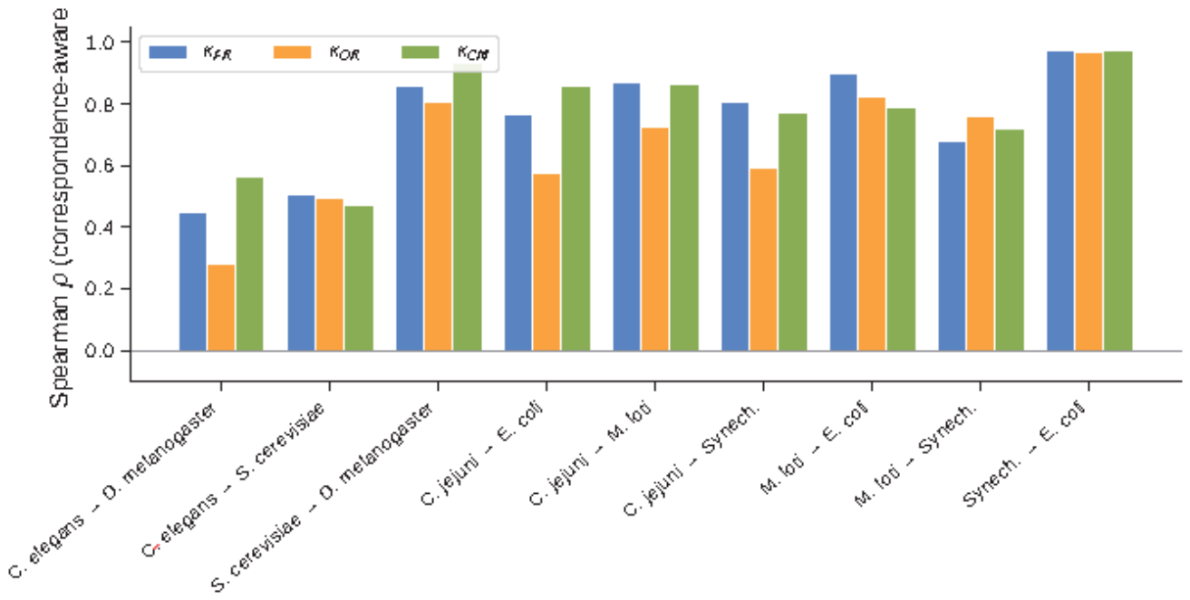
Figure 2.
Correspondence-aware Spearman agreement for (blue), (orange), and (green), averaged over all comparisons within each organism pair. Values near 1 indicate that both alignments preserve the same curvature ordering; values near 0 indicate no consistent curvature transformation.
Figure 2.
Correspondence-aware Spearman agreement for (blue), (orange), and (green), averaged over all comparisons within each organism pair. Values near 1 indicate that both alignments preserve the same curvature ordering; values near 0 indicate no consistent curvature transformation.
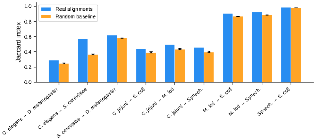
Figure 3.
Curvature distributions induced by two alignments on (H, blue) and (K, orange) for two representative organism pairs (rows) and three curvatures (columns). and produce signed, heavy-tailed distributions; produces strictly positive distributions.
Figure 3.
Curvature distributions induced by two alignments on (H, blue) and (K, orange) for two representative organism pairs (rows) and three curvatures (columns). and produce signed, heavy-tailed distributions; produces strictly positive distributions.
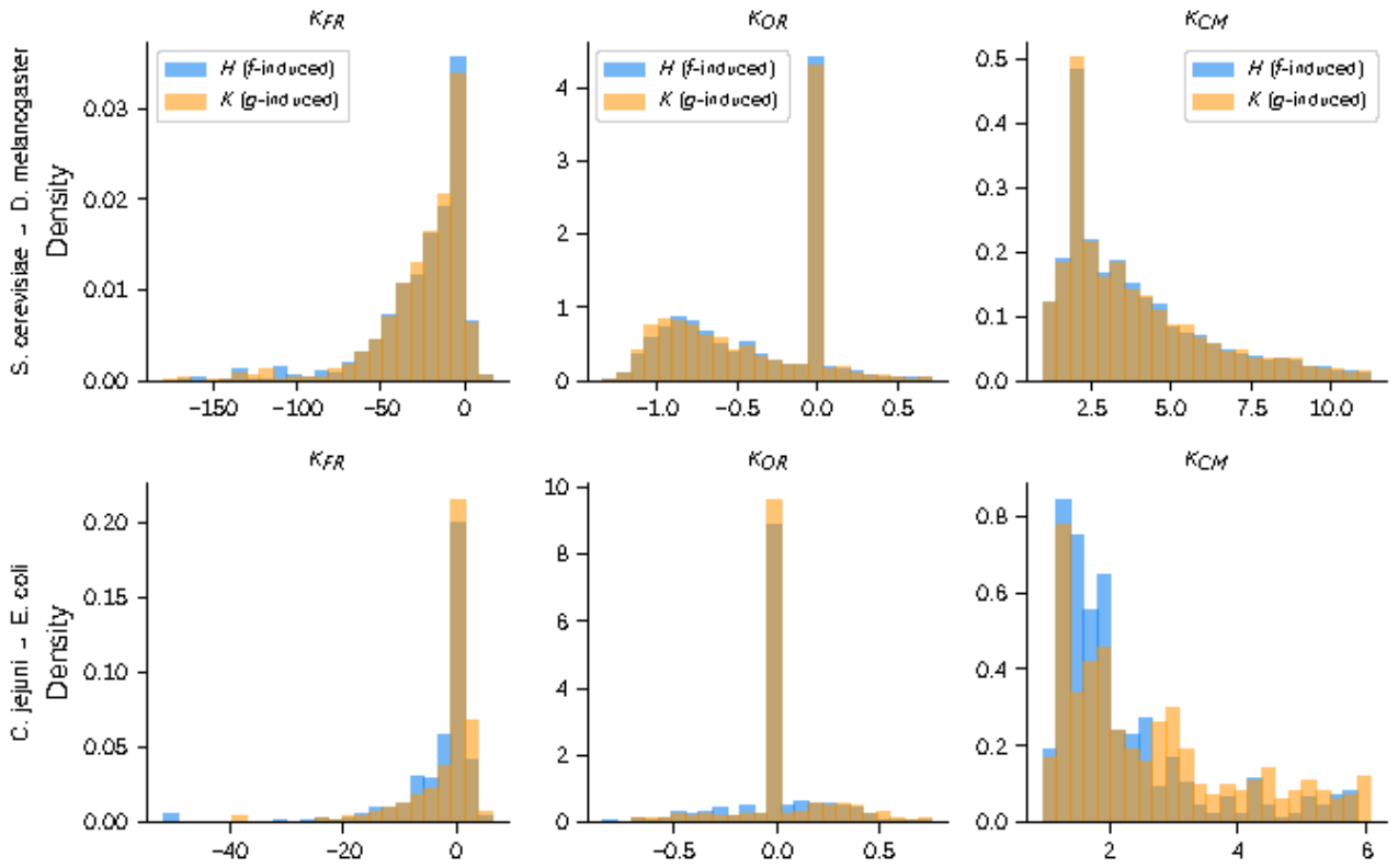
Figure 4.
Spearman correlation between the three discrete curvatures, computed on H-induced node curvature values for three representative organism pairs. and are strongly correlated; is largely independent.
Figure 4.
Spearman correlation between the three discrete curvatures, computed on H-induced node curvature values for three representative organism pairs. and are strongly correlated; is largely independent.
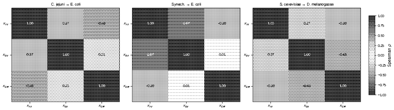
Figure 5.
Total pipeline time per comparison (all curvatures) versus network size . Circles: comparisons where is feasible (FR + OR + CM). Triangle: H. sapiens, where is skipped (FR + CM only). The H. sapiens network () completes in ∼203 s.
Figure 5.
Total pipeline time per comparison (all curvatures) versus network size . Circles: comparisons where is feasible (FR + OR + CM). Triangle: H. sapiens, where is skipped (FR + CM only). The H. sapiens network () completes in ∼203 s.
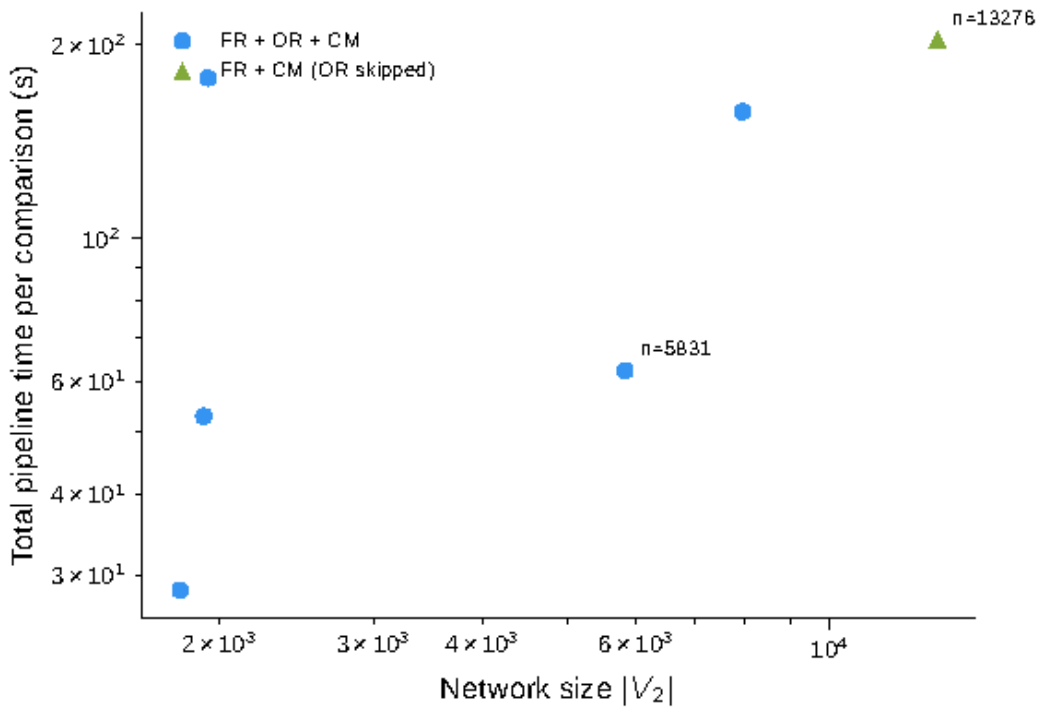
Figure 6.
Agreement measures versus orthology recovery fraction. Left: Jaccard index. Center: Spearman for . Right: Spearman for . Orthology recovery is uniformly low across all agreement levels.
Figure 6.
Agreement measures versus orthology recovery fraction. Left: Jaccard index. Center: Spearman for . Right: Spearman for . Orthology recovery is uniformly low across all agreement levels.
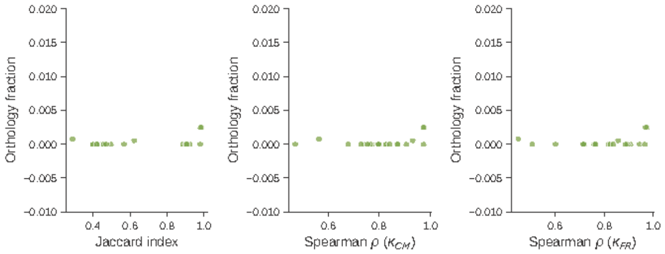

Table 1.
Computational complexity of curvature computation and agreement measurement. , , = max degree, k = truncation rank.
Table 1.
Computational complexity of curvature computation and agreement measurement. , , = max degree, k = truncation rank.
| Component | Exact | Approximate |
|---|---|---|
| (per graph) | — | |
| (per graph) | — | |
| (per graph) | ||
| (per pair) | — | |
| (per pair) | — |
Table 2.
Networks used in this study.
| Organism | Code | Nodes | Edges |
|---|---|---|---|
| C. jejuni | cjejuni | 1,095 | 2,988 |
| E. coli | ecoli | 1,941 | 3,989 |
| M. loti | meso | 1,804 | 3,094 |
| Synechocystis | syne | 1,920 | 3,102 |
| C. elegans | CElegans | 3,134 | 5,428 |
| S. cerevisiae | SCerevisiae | 5,831 | 77,149 |
| D. melanogaster | DMelanogaster | 7,937 | 34,753 |
| H. sapiens | HSapiens | 13,276 | 110,528 |
Table 3.
Permutation test: real Jaccard vs. random null. z-score and two-tailed p-value from normal approximation.
Table 3.
Permutation test: real Jaccard vs. random null. z-score and two-tailed p-value from normal approximation.
| Pair | z | p | ||
|---|---|---|---|---|
| cjejuni_ecoli | 0.421 | 0.393 | 2.90 | 0.004 |
| cjejuni_meso | 0.476 | 0.436 | 4.22 | |
| cjejuni_syne | 0.427 | 0.399 | 2.89 | 0.004 |
| meso_ecoli | 0.895 | 0.868 | 9.43 | |
| meso_syne | 0.910 | 0.886 | 10.00 | |
| syne_ecoli | 0.982 | 0.979 | 7.27 | |
| CElegans_SCerevisiae | 0.568 | 0.368 | 34.94 | |
| CElegans_DMelanogaster | 0.289 | 0.246 | 8.13 | |
| SCerevisiae_DMelanogaster | 0.623 | 0.581 | 11.42 |
Table 4.
Intra-method bacterial agreement: SANA42 vs. SANA137. J = Jaccard, = Spearman agreement.
| Pair | J | |||
|---|---|---|---|---|
| cjejuni_ecoli | 0.439 | 0.818 | 0.571 | 0.907 |
| cjejuni_syne | 0.460 | 0.898 | 0.642 | 0.771 |
| cjejuni_meso | 0.497 | 0.946 | 0.775 | 0.871 |
| meso_ecoli | 0.908 | 0.909 | 0.840 | 0.799 |
| meso_syne | 0.923 | 0.716 | 0.775 | 0.754 |
| syne_ecoli | 0.987 | 0.977 | 0.973 | 0.978 |
Table 5.
Cross-method bacterial agreement: SANA42 vs. MAGNA++.
| Pair | J | |||
|---|---|---|---|---|
| cjejuni_ecoli | 0.422 | 0.759 | 0.587 | 0.830 |
| cjejuni_syne | 0.401 | 0.760 | 0.553 | 0.743 |
| cjejuni_meso | 0.459 | 0.826 | 0.705 | 0.873 |
| meso_ecoli | 0.890 | 0.896 | 0.821 | 0.764 |
| meso_syne | 0.901 | 0.601 | 0.735 | 0.678 |
| syne_ecoli | 0.980 | 0.970 | 0.964 | 0.973 |
Table 6.
Eukaryote agreement: SANA42 vs. SANA137. The C. elegans → H. sapiens pair demonstrates scalability to 13K-node networks; is omitted for H. sapiens (max degree 1957 makes optimal transport infeasible).
Table 6.
Eukaryote agreement: SANA42 vs. SANA137. The C. elegans → H. sapiens pair demonstrates scalability to 13K-node networks; is omitted for H. sapiens (max degree 1957 makes optimal transport infeasible).
| Pair | J | |||
|---|---|---|---|---|
| CElegans_SCerevisiae | 0.568 | 0.505 | 0.495 | 0.471 |
| CElegans_DMelanogaster | 0.289 | 0.447 | 0.281 | 0.564 |
| SCerevisiae_DMelanogaster | 0.623 | 0.857 | 0.808 | 0.932 |
| CElegans_HSapiens | 0.200 | 0.547 | — | 0.535 |
Disclaimer/Publisher’s Note: The statements, opinions and data contained in all publications are solely those of the individual author(s) and contributor(s) and not of MDPI and/or the editor(s). MDPI and/or the editor(s) disclaim responsibility for any injury to people or property resulting from any ideas, methods, instructions or products referred to in the content. |
© 2026 by the authors. Licensee MDPI, Basel, Switzerland. This article is an open access article distributed under the terms and conditions of the Creative Commons Attribution (CC BY) license (http://creativecommons.org/licenses/by/4.0/).
Copyright: This open access article is published under a Creative Commons CC BY 4.0 license, which permit the free download, distribution, and reuse, provided that the author and preprint are cited in any reuse.