

Submitted:
30 July 2026
Posted:
31 July 2026
You are already at the latest version
Abstract
Small-area population data underpin efficient resource allocation but are often unavailable where censuses are outdated or absent. We present a generalizable geostatistical model-based computational technique for estimating population counts from limited, imperfectly observed health intervention campaign data. The approach embeds a robust data cleaning strategy while integrating geolocated population enumerations with satellite-derived building footprints and geospatial covariates within a Bayesian Hierarchical modelling framework. Using real data application and a simulation study implemented over a range of biasedness and missingness scenarios, we evaluated three data cleaning strategies and showed that the approach involving exclusion of biased samples from the training set, produced the smallest estimation errors in both simulation studies (1.5% to 65.7% reductions in relative mean absolute error (RMAE)) and when used in prediction modelling from recent geolocated malaria bednet campaign data in Nigeria (17.1% reduction in RMAE). This approach which enabled us to generate gridded and administrative unit-level population estimates (total national estimate ~ 237.4M; 95%CI 233.6M – 243.7M people) from imperfect operational data across Nigeria is transferable to other data-scarce settings.
Keywords:
census-independent
; small area population estimates
; Bayesian hierarchical modelling
; geostatistical methods
; bias correction
; health campaign data
Introduction
The availability of timely and reliable small-area population estimates is crucial for effective government policies and humanitarian efforts [1]. Such spatially detailed data, which provide robust statistical evidence for equitable resource allocation, infrastructural development, targeted health interventions, census preparations, and disaster management efforts [2,3] are available in most countries through various sources, including decennial censuses, administrative records, and regular surveys. However, in countries experiencing prolonged instability, significant population changes, and resource constraints, a lack of recent enumeration and weak administrative systems can mean that reliable small-area population data are lacking [4].
Over the past decade, Bayesian statistical population modelling methods which combine geolocated sample enumeration data with satellite-derived settlement maps and geospatial covariates to produce nationwide small-area population estimates with uncertainty metrics have been developed [5,6,7,8,9,10,11,12]. These so called ‘bottom-up’ population models [13] assess the spatial relationship between population density based on the enumeration data and satellite-derived human settlement data with other geographically located factors that describe human population distribution, to predict populations counts at small area level across the entire spatial domain of interest, including in the settlements where no enumeration data were collected [7]. These factors include nighttime light intensity, building density, climatic factors and land use/land cover variables. Model parameter estimates are based on Bayesian statistical inference either through a Markov chain Monte Carlo (MCMC) algorithm-based methods [6,8] or through the integrated nested Laplace approximations (INLA) frameworks [9,10,11,12].
Bottom-up population models have been successfully developed and applied in various contexts using sample enumeration datasets from microcensuses (custom, full enumeration of small areas) [6,8], partial (incomplete) censuses [14] or household surveys [9,10,11]. Where these are unavailable, recent applications have explored the use of healthcare intervention campaign data [12]. However, like most household survey datasets, these health campaign-derived datasets may only cover the area of interest partially, especially where insecurity makes some areas inaccessible. The use of sparsely distributed datasets within existing modelling frameworks can result in highly uncertain estimates. Also, the inherent reporting biases that can be commonplace in health campaign data [15,16,17] potentially pose additional challenges for robust planning.
In this paper, we develop a bespoke Bayesian hierarchical modelling approach and test integrated data-cleaning strategies to evaluate the feasibility of producing reliable small-area population estimates from partial health campaign data. We demonstrate its application through the production of population estimates at both 100 m grid-square scale and different subnational administrative unit levels for the entirety of Nigeria utilising 2022/2023 National Malaria Elimination Programme (NMEP) bednet distribution campaign data.
Methods
In this section, we provide details on datasets used as well as the background of the proposed methodology. Figure 1 shows the workflow of the modelling framework.
Figure 1 highlights that datasets including health campaign data (household/point scale), satellite-derived settlement data (gridded) and geospatial covariates (gridded) are initially processed and cleaned. The second stage involves preliminary analysis to examine relationships between the geospatial covariates and population density, checking for multicollinearity at modelling unit scale (ward level). Covariate selection relies on generalized linear model (GLM)-based stepwise regression, and multicollinearity is assessed by calculating the variance inflation factor (VIF) values of the covariates. The Bayesian models are selected based on their deviance information criteria (DIC) with models having smaller DIC values selected as the best fit models. Further checks on predictive ability are performed using cross-validation at modelling-unit scale. Finally, population predictions are made at 100 m grid cells along with the corresponding estimates of uncertainty, as well as aggregations to administrative unit levels.
Study Domain and Data
Geographically, Nigeria is divided into 36 States and the Federal Capital Territory (FCT) at administrative level 1 and further divided into local government areas at level 2 and wards at level 3. Figure 2 shows the states and wards with observed campaign-based enumeration data.
The input data consisted of three key types, namely, i) demographic data, containing the counts of people at geo-referenced small-area units in Nigeria observed through an anti-malaria bednet distribution campaign, as well as subnational age-sex proportions from official projections; ii) satellite imagery-based settlement maps covering the entire country which provide indications of where and how humans are distributed on the Nigerian landscape; and iii) a set of geospatial covariates related to population density obtained from multiple sources. Further details of each of the datasets are provided below, with additional information on the geospatial covariates given in Table S1 of the supplemental materials.
Demographic Data
Datasets containing household counts collected during the 2022/2023 nationwide anti-malaria bednet distribution campaign in Nigeria were provided by the National Malaria Elimination Programme (NMEP). At the time of this study, only data from 9 out of the 36 Nigerian States and the FCT were provided, as shown in Figure 2. Average number of people per household (pph) ranged from 4.99 people in Kaduna to 6.08 in Kwara State. Using the ward boundaries provided by GRID3 (https://data.grid3.org/), the anonymized geolocated household-level data were aggregated to the ward level which served as the training unit so that individual households are not identifiable.
The NMEP data do not contain information on age-sex breakdowns, therefore we used the 2022 National Population Commission (NPC) subnational population projections broken down by age and sex to calculate the age-sex proportions per state [18].
Satellite Imagery-Based Settlement Maps
Satellite-derived human settlement data used in this study were provided by the Center for Integrated Earth System Information (CIESIN), Columbia University for GRID3 [19]. The settlement data are outputs from advanced machine learning algorithms that integrate multiple sources of human settlement data [21]. They are provided as gridded maps with 2024 as the reference year and are used to inform the statistical models on where and how human settlements are distributed across the Nigerian landscape. Specifically, the settlement datasets contain information on the building area and building counts for each grid square of approximately 100 m × 100 m (i.e., approximately 3 arc-seconds) in size and cover the entire country. Here, building area is the total area of buildings whose centroids fall within a given grid cell; while building count is the number of buildings whose centroids fall within that grid cell.
Geospatial Correlates of Population Density
For statistical modelling, we explored a range of geospatial covariates known to correlate with population density and distribution [20]. These covariates are required for training the model parameters to facilitate the prediction of population density and counts in locations where no input enumeration data were available. They include land use and land cover variables, climate variables such as temperature and rainfall, and physical features and infrastructure, such as distances to roads, health facilities, schools, and conflict-area indicator variables. Table S1 of supplementary information outlines the 55 datasets that were assembled and explored.
To ensure that the corresponding regression coefficients of these covariates, which often differ in their units of measurement, are comparable, all continuous geospatial covariates were standardized using the z-score. This was done by dividing the difference between the covariate value and the mean by the corresponding standard deviation , i.e., .
We took additional steps to remove redundant covariates and minimize the potential effects of multicollinearity by first selecting the best set of model covariates using a generalized linear model (GLM)-based stepwise selection method21. The selected covariates were then assessed for multicollinearity by calculating the variance inflation factor (VIF), and only those with VIF < 5 were retained for the final Bayesian hierarchical modelling and prediction (see also Section S1.1 in the SI document).
The geospatial covariates were obtained from different sources and time periods (Table S2 of the Supplementary document), spanning mostly from 2021 to 2023. Of the 55 initially explored geospatial covariates, the final six covariates retained that had the strongest correlations with the population density data at ward level are: distance to cropland and natural vegetation (cov1), distance to tree cover (cov2), annual average precipitation (cov3), annual average temperature (cov4), distance to the edges of International Union for Conservation of Nature strict nature reserves and wilderness areas (2015–2022) (cov5), and evolution of settlement (cov6).
Data Preparation and Cleaning
The NMEP data were cleaned to remove unrealistic counts and aggregated to the ward level, which formed the training units for the statistical model parameters. Other associated datasets were also aggregated to the ward level, including the geospatial covariates and the human settlement datasets. The mean values of continuous covariates across all grid cells within a given ward were calculated and used as the corresponding ward-level values, while building counts were aggregated as the sum of all buildings across the grid cells within each ward.
The NMEP data assume complete enumeration of all individuals living in each of the states provided. However, preliminary exploratory analysis indicated missing household points in some states, as well as household points with coordinates outside their respective states. Additionally, the geolocated population data points were observed to be unevenly distributed across the satellite-derived settlement extents, with clusters of household data points falling into uninhabited areas when overlaid with recent satellite imagery. Most household points located outside of their assigned states were observed in Katsina, Kano, Niger, Taraba, and Delta, with more than six thousand households points in Delta state falling outside the boundaries of the State. As Nigeria is covered by three UTM zones it was assumed that this led to some of these geolocating process inaccuracies. Thus, household points falling outside a given state were therefore relocated to the closest ward of their respective state.
We explored three data cleaning strategies, namely Base, Imputed, and Dropped (Figure 2b–d). The Base training dataset was produced by simply excluding (i) household points that fell outside their respective states and wards, (ii) wards with no observed NMEP population or (iii) wards where CIESIN had no building counts (i.e., non-settled). First, to ensure consistent data cleaning, the observed input household enumeration data were rasterized into 100m grid cells. The Imputed cleaning strategy first replaces any observed total NMEP population count greater than 1,000 people per grid cell in a given ward with the median of the observed total counts across all the grid cells within the same ward. Note that the choice of 1000 people as the threshold is based on the WorldPop Global 202420 maximum pixel estimate for Nigeria (414 people) and allowed for some flexibility to account for variabilities in the dataset. This was implemented across 1161 wards.
In the second step, we imputed pixel population count values where the population density (NMEP observation divided by CIESIN building count) exceeded 100 people per building with the median observed population count of the nearest pixels, thereby allowing us to take building counts into consideration. This was done by using a focal window calculation with the window size initially set to be approximately 500m radius (5x5 pixels), and if a valid (i.e., not NA) median value was not found within that area, we expanded the focal window gradually (adding one pixel to each direction of the focal window) until we found a valid median value. Compared to the raw observations, this resulted in a change to 61% of the wards.
The Dropped cleaning strategy used ward-level summaries of the NMEP observations and compared them with ward-level summaries of the CIESIN building counts [19] and WorldPop Global population estimates for 2023 [22]. Wards were dropped if the NMEP population per building was less than one or greater than 20, or if the WorldPop-to-NMEP population count ratio was less than 0.4. This implies that the NMEP observation was at least 2.5 times larger than the WorldPop estimate for that ward, potentially indicating significant positive bias (i.e., overreporting or inflation of household sizes). Eventually, the Dropped strategy resulted in dropping 434 wards.
We used a Bayesian hierarchical regression model and k-fold cross-validation to evaluate the prediction accuracies of the statistical models based on each of the three datasets, with more background details provided below.
Statistical Modelling
The population count for a given ward is assumed to follow a Poisson distribution with mean , such that . However, the Poisson likelihood requirement of equal mean and variance, i.e., , is rarely met in the context of small-area population modelling [6,8,9,10,11,12,14]. As a result, the mean parameter is often reparameterised as , where is the total number of buildings within ward and is the mean population density estimated from , such that
That is, the population density is defined as the number of people per building and follows a Gamma distribution given by
where and are the shape and rate parameters, with mean and variance , respectively. The predicted population density forward is then given by
where and are the design matrices of fixed-effect covariates (e.g., average annual precipitation, average annual temperature, distance to cropland) and random effects (e.g., settlement type, state, LGA), respectively. The terms and are the vectors of fixed-effect regression parameters and random-effect variances, respectively.
The terms and are the spatially varying and spatially independent random effects accounting for spatial autocorrelations and spatial independence between observations in spatially contiguous wards, respectively.
We model as a zero-mean Gaussian Random Field (GRF) given by
where is a dense covariance matrix. For computational efficiency, is evaluated using the Integrated Nested Laplace Approximation (INLA [21,22,23]) approach in conjunction with the Stochastic Partial Differential Equation (SPDE [24]) method (INLA–SPDE). This approach allowed us to approximate the dense GRF with a sparse Gaussian Markov Random Field (GMRF) by discretizing the continuous spatial domain using a mesh. In addition, we modelled the term as zero-mean Gaussian noise, specified by
where is a variance parameter.
In the context of the NMEP–Nigeria datasets, wards (Admin 3) were used as the model training units. All models were implemented within a Bayesian inference framework using the R-INLA package, and the overall hierarchical model was given by
where is the linear predictor; are the fixed-effect regression parameters of the final geospatial covariates; and are zero-mean random effects capturing state- and LGA-specific differences in the observations; is the projection matrix that maps the observations to the vertices of the mesh triangulation; is a realization of the GMRF; and is as defined in Equation (5), with .
Prior: To ensure flexibility and better capture local variability within the data, we applied Penalized Complexity (PC) priors to the standard deviation parameters throughout, such that a small probability of 0.01 is assigned to the event that the standard deviation exceeds 1, i.e., .
Grid-cell prediction: We used the corresponding grid-cell scaled values of the geospatial covariates, provided at 100 m × 100 m resolution across grid cells covering the entire country, to predict the population density per grid cell . Then, together with the corresponding building count for each grid cell, the predicted population count at grid cell is obtained as
Model Fit Metrics
Mean Absolute Error (MAE): The mean absolute error (MAE) provides a measure of the average magnitude of errors in a set of predictions, irrespective of their direction. It is calculated using
Where and are the observed and predicted values, respectively. The model with the smaller MAE provides a better fit.
Percentage Reduction in Relative MAE (RMAE): The percentage reduction in RMAE provides a measure of the prediction accuracy of the proposed model compared with the base model, based on their respective MAE values. A positive value indicates higher accuracy of the proposed method over the base model—the larger the value, the more accurate the prediction. It is calculated using Equation (9):
where and are the mean absolute error values of the predicted population counts based on the proposed and base methods, respectively.
Root Mean Square Error (RMSE): The root mean square error (RMSE) is like the MAE in that it provides an idea on the average magnitude of prediction error. However, the RMSE is found to be more useful when large errors are not desirable. RMSE is given by
Like the MAE, models with smaller RMSE values provide better fit.
Pearson correlation coefficient (): The Pearson correlation coefficient ) is the coefficient of correlation between the observed and predicted counts.
where and are the observed counts, mean of the observed counts, the predicted counts, and the mean of the predicted counts, respectively.
Coefficient of Variation (CV): For each posterior sample, we computed the coefficient of variation (CV) as a measure of uncertainty in the posterior parameter estimation. It is given by
where a smaller value of CV indicates more accurate prediction.
Model performances were tested based on equation (13) which provided the predicted population density from the best fit model across the three data-cleaning strategies evaluated
Aggregation to Administrative Units
R-INLA allows us to obtain posterior draws from the posterior distribution of the parameters given the data :
where and hyperparameters are the latent field and hyperparameter, respectively. The posterior draws are obtained using the inla.posterior.sample() function after setting the argument control.compute = list(config = TRUE) within the inla() function of the R-INLA package [25]. Then, following equations (7) and (13), the predicted population density and the predicted population counts at each grid cell for each draw are given by:
and
This then produces a sample distribution of the predicted grid total population over the posterior samples The corresponding posterior samples for administrative unit over the draws are also obtained , where , is the aggregated total population count for administrative unit from all the grid cells within .
Then, the availability of the distributions from the posterior samples at both grid and administrative units make it straightforward to obtain summary statistics such as the mean and median as well as measures of uncertainties such as the standard deviation, 95% quantiles and coefficient of variation (CV). Thus, at both grid and administrative unit levels, the mean predicted total counts are obtained using the respective samples as
where is a generic index for the grid cell or the administrative unit so that is the mean total predicted counts for grid , while is the mean total predicted counts for administrative unit . In all cases, it is expected that the overall national population total aggregated from either across all the grid cells or the administrative units be equal, that is, .
Similarly, the uncertainty metrics are derived from posterior draws as follows:
where is the predicted total grid population for draw , and is the aggregated predicted total grid populations at draw across all the grid cells belonging to administrative unit ; and are the corresponding lower and upper bounds of the 95% credibility interval obtained using the quantile() function while setting probs = 0.025 for the lower bound and probs = 0.975 for the upper bound; , , and are the standard deviation, the relative credible interval and the coefficient of variation, respectively. Aggregation on posterior draws preserves coherent totals and correctly propagates uncertainty across scales, especially because sum of quantiles is not the same as the quantile of sums.
Results
Simulation Study
Datasets (population counts, building counts, geospatial covariates) were simulated for the 6,733 rectangular grid cells remaining after cropping the initial 10,000 prediction grid cells to the spatial extent of Nigeria using the national boundary (Figure S1). The simulation study parameters are shown in Table S2. Briefly, datasets were initially simulated with the “true” parameter values and then allowed to vary in quality, such that of the observations were missing at random, and of the remaining , were biased with magnitude of bias, where , , and . Thus, implies that of the 90% of all samples observed, 40% were biased with a 20% magnitude of bias for each sample. We define the magnitude of bias as the percentage overcount relative to the “true” value; for example, a population size of 120 people has a 20% magnitude of bias if the “true” value is 100 people.
Figure 3a and Figure 3b compare the mean absolute error (MAE) and Pearson correlation coefficient (CC) values obtained across the 125 data quality scenarios for the three data treatment/cleaning strategies employed. In general, prediction accuracy decreased as the proportion of biased population and the magnitude of bias increased. The results show that the Bayesian hierarchical models based on the Imputed and Dropped strategies consistently provided better fits (lower MAE and higher CC values) than the Base approach. However, the overall best fit was achieved by the Dropped strategy, which also produced reductions in relative mean absolute error (RRMAE) ranging from 1.5% to 65.7% when compared with the Base strategy (see also Figure S2 of the Supplementary Information document).
Application to the Nigeria Dataset
We applied the Bayesian hierarchical modelling framework using the available NMEP health campaign data from nine states and produced gridded population estimates across Nigeria at 100 m × 100 m spatial resolution.
Posterior Fixed Effects Parameter Estimates
Following rigorous multi-layer covariate selection strategies – particularly through stepwise regression and variance inflation factor–based metrics – the fixed-effect estimates of the final six geospatial covariates retained are shown in Table 1. These estimates are based on the best-fit model specified in Equation (13) across the three data treatment strategies we explored. The results show some variation in the posterior estimates of the fixed-effect parameters across the different data-cleaning strategies; however, the ranges of the values, in terms of the 95% credible intervals, are generally similar.
Model Fit Metrics and Spatial Distribution of Posterior Estimates Across Administrative Units
Figure 4 compares the cross-validated results obtained across the three data treatment/cleaning strategies employed. Specifically, Figure 4a, which shows scatter plots of observed versus predicted values, indicates that the Dropped approach provided the most coherent predictions, with more predicted values closely aligning with the observations. Figure 4b, Figure 4c and Figure 4d show that both the Imputed and Dropped strategies outperformed the Base approach, with lower cross-validated mean absolute error (MAE) and root mean square error (RMSE) values, as well as higher Pearson’s correlation coefficient (CC). However, consistent with the simulation study results, the Dropped strategy provided the overall best fit and produced a 17.1% reduction in relative mean absolute error (RRMAE) compared with the Base method.
Spatial Cross-Validation
To evaluate out-of-sample predictive performance while accounting for spatial autocorrelation, we implemented spatial cross-validation [26] to the best fit model of the Dropped strategy. Conventional random cross-validation can overestimate predictive accuracy when observations are spatially correlated. Therefore, survey clusters were partitioned into geographically contiguous folds using spatial blocking. This was achieved by dividing the dataset into five spatial folds using square blocks of approximately 50 km × 50 km to ensure spatial independence between training and validation datasets.
In each iteration, the model was trained on four folds and predictions were generated for the held-out fold. This process was repeated until all folds had served as validation data. Predictions at validation locations were obtained from the posterior predictive distribution of the fitted INLA-SPDE model. Predictive performance was assessed by comparing observed and predicted population density/population count at held-out locations and we calculated the MAE, RMSE, and CC values. Additionally, we evaluated uncertainty calibration by calculating the proportion of observed values falling within the 95% posterior credible intervals.
Results indicated strong predictive performance with RMSE = 14,104; MAE = 8,332; CC = 81.2%) for population count. The 95% credible intervals showed good calibration, with a coverage probability of 0.943 indicating that ~94.3% of the observed population counts are within the 95% credible interval of the posterior predictions.
Gridded High-Resolution Population Estimates
We used the grid-cell values of the geospatial covariates retained in the best-fit model, along with the building counts per grid cell, to produce estimates of population counts for 2023/2024 across 7,185,917 settled grid cells at 100 m spatial resolution in Nigeria. These estimates were provided along with the corresponding coefficient of variation (CV) as a robust measure of uncertainty at the grid-cell level (Figure 5 of the Supplementary Material; Figure 5a shows the mean, while Figure 5b shows the corresponding CV). The CV was calculated by dividing the standard deviation of the predicted population count by its mean value, allowing us to evaluate the predictive performance of our methodology. Predictions across grid cells with higher CV values are more uncertain than those with lower CV values.
Aggregated Population Totals
Our methodology allowed us to produce aggregated total population counts at subnational levels – across wards, local government areas, and states – along with the corresponding 95% credible intervals and measures of uncertainty estimated using the coefficient of variation (CV). The aggregation used all posterior simulations of a pixel and summed these up to various administrative levels. This enabled to accurately transfer the estimated uncertainties to admin units. The CV was calculated by dividing the standard deviation by the mean (Figure 5c–h).
In all cases, population estimates were provided across the entire country, including the remaining 27 states and the FCT, where no input population data were available. Moreover, our methodology enabled quantification of uncertainties across the country. Results indicate moderate uncertainties overall, which were higher in wards with no input population data but decreased gradually as the spatial aggregation increased. Consequently, lower magnitudes of uncertainty (higher accuracy) were observed at the state level compared with local government areas and ward levels.
The approach estimates the total national population of Nigeria in 2023/2024 to be 237,345,980 people. Under the 95% credible interval (CI), we estimate that the “true” total national population lies between 233,596,990 people at the lower bound (2.5%) and 243,655,702 people at the upper bound (97.5%). These estimates are close to projections from other sources. For example, the United Nations World Population Prospects projects a total national population of approximately 237,500,000 people for Nigeria in 2025 [27], while the National Population Commission projects 232,676,020 people for 2025 using the Cohort-Component method [18].
Although estimates of uncertainty were generally low across the states, the highest levels of uncertainty were mostly observed in LGAs where no demographic data were available. These include LGAs in Akwa Ibom, Bayelsa, Rivers, Ekiti, Borno, Bauchi, Yobe, Zamfara, and Sokoto States. However, high uncertainty estimates were also observed in some LGAs with available demographic data, such as in the western parts of Delta State. This is likely attributable to the heterogeneity in settlement patterns and input population data across these regions.
The modelled population estimates were further disaggregated by age and sex by multiplying the estimated population counts with the corresponding subnational age-sex proportions based on the NPC datasets [18]. These proportions were then applied to our gridded population estimates to produce gridded estimates disaggregated by age and sex at 100 m spatial resolution.
However, because only State-level subnational age-sex projections from the NPC were available for disaggregation, all grid cells within a given state have identical age and sex proportions. The disaggregated data were then used to produce age-sex pyramids across 18 age classes (see Figure S5 of the Supplementary Document). The age classes represent commonly reported sequential five-year age groups for males and females, along with four additional demographic groups often targeted by programs and interventions: children under 1 year, children under 5 years, children under 15 years, and females aged 15–49 years.
Discussion
This study was motivated by the absence of recent, reliable small-area population data to support national and subnational evidence-based operational planning and resource allocation in Nigeria. We developed and implemented a bespoke bottom-up population modelling framework and produced high-resolution population estimates for Nigeria at 100 m grid cells, with 2023/2024 as the reference period. By jointly using the Integrated Nested Laplace Approximation (INLA) [22,23] and Stochastic Partial Differential Equation (SPDE) [24] techniques, we combined satellite-derived human settlement data with sparsely distributed health campaign data from the National Malaria Elimination Programme (NMEP). The human settlement data, containing the number of buildings within a given area unit, were used to define population density. Together with a stack of geospatial covariates, we trained a robust Bayesian hierarchical regression model, which allowed us to produce population estimates at 100 m grid cells across the entire country, including areas with no input demographic data.
The use of the INLA–SPDE framework in the context of small-area bottom-up population modelling, along with Penalized Complexity (PC) priors [28] to better capture localized variability, represents a key methodological advancement in data-limited settings. In addition, it allows for the incorporation of spatial autocorrelation [10,29] and multiple random effects within the model, thereby capturing both spatial and hierarchical structures in the input datasets. This approach yields statistically robust predictions along with estimates of uncertainty. The resulting posterior distributions from the Bayesian inference implemented through INLA provide not only point estimates but also measures of confidence, which are critical for effective decision-making. The estimated population of Nigeria in 2023/24 using these methods is 237,345,980 people with a 95% credible interval (CI) of 233,596,990 and 243,655,702. Considering that the last census was in 2006 and the size of the national population, the 10 million people range of potential values is reasonably narrow to make robust policy and operational decisions. However, with more recent and more complete datasets, we hope to obtain more accurate estimates with significantly narrower credible intervals.
The data-cleaning strategy used in this study, evaluated through a simulation study, effectively addressed inconsistencies and outliers in the input datasets, improving the accuracy and reliability of model parameter estimates. Results indicated that excluding inconsistent samples from the training sets (Dropped strategy) provided the overall best fit, resulting in reductions in relative mean absolute error (RRMAE) of between 1.5% and 65.7% in the simulation study, and 17.1% when applied to the Nigerian data. This proves that such operational data sources, not designed originally for statistical analyses, can be valuable for census-independent small area population estimation.
While the statistical modelling techniques employed offer significant advantages, some key limitations should be acknowledged. First, the estimation process allocates population only within grid cells identified as settled based on satellite-derived building footprints. Therefore, the accuracy of modelled estimates may be affected by changes in settlement patterns; for example, settlements that have recently emerged or been abandoned due to displacement, conflict, or rapid urban expansion may lead to under- or overestimation of population counts in specific grid cells. Second, despite the implemented cleaning steps, uncertainties in the modelled estimates may be influenced by inaccuracies in the input demographic data from NMEP, as well as differences in data collection years. While the SPDE approach allows the model to “borrow strength” from locations with observations to estimate population counts in neighbouring areas with few or no observations, it does not fully address sample representativeness across Nigeria, especially given that datasets from only 9 of the 36 states and the FCT (~24% coverage) were included. Variations at lower administrative unit levels may therefore not have been fully captured. Another limitation of this study is that age–sex structures were assumed to be spatially homogeneous within each State. Because sub-state demographic data were unavailable, State-level age–sex proportions from the National Population Commission projections were applied uniformly across all grid cells, which mask within-state demographic heterogeneity (e.g., urban–rural differences). Finally, mobile populations, such as seasonal migrants or nomadic communities, which were not explicitly integrated into the model framework, may contribute to biases, particularly in dynamic population contexts.
The inclusion of recent NMEP demographic data and information on settlement evolution as model covariates helps mitigate some of the challenges outlined above. These inputs allow the model to capture recent patterns in population density and distribution, reducing potential biases arising from temporal lags in settlement data. Improvements in the frequency and accuracy of satellite-based settlement mapping will further enhance the temporal responsiveness of bottom-up models like the one implemented in this study. By combining satellite-derived settlement data with regionally available empirical health campaign data, our methodology bridges the gap between remotely sensed datasets and ground-based population information.
Given that Nigeria’s last national population and housing census was conducted 20 years ago (2006), approaches to construct reliable and contemporary small-area population estimates remain critical for national planning and governance. The population estimates produced in this study offer a valuable data source to support census preparations, interim demographic assessments, and humanitarian operations. By providing spatially detailed and statistically rigorous estimates disaggregated by age and sex, these data can support pre-census mapping, guide field verification, and inform the prioritization of enumeration activities. Beyond census applications, the high-resolution gridded population surfaces are relevant for public health microplanning, infrastructure development, and emergency response, especially in rapidly changing or hard-to-reach areas [3,30,31].
Supplementary Materials
The following are available online at www.mdpi.com/xxx/s1, Figure S1: title, Table S1: title, Video S1: title.
Author Contributions
Conceptualization: CCN; Data Curation: CCN, AG, ANL; Formal Analysis: CCN, AG, ANL; Methodology: CCN; Project Administration: ANL, AJT; Software: CCN; Supervision: ANL, AJT; Writing - original draft: CCN; Writing – review & editing: CCN, AJT, ANL, AG, OO, HRC.
Funding
These data were produced by the WorldPop Research Group at the University of Southampton as part of the GRID3 – Phase 2 Scaling project, with funding from the Gates Foundation (INV-044979). Project partners included GRID3 Inc., the Center for Integrated Earth System Information (CIESIN) within the Columbia Climate School at Columbia University, and WorldPop at the University of Southampton.
Institutional Review Board Statement
The analyses outlined in this paper were approved by the Ethics and Research Governance Online of the University of Southampton (submission ID: 94380).
Data Availability Statement
The input demographic and administrative datasets used in this study were provided by the NMEP and requests for these datasets may be sent to the NMEP team through https://nmcp.gov.ng/contact/. The final geospatial covariates used in the modelling can be downloaded from the various links provided in Table S2 of the supplementary document. The small-area population estimates produced for Nigeria using the methods outlined above and adjusted to match UN World Population Prospects 2024 national estimates can be downloaded from WorldPop’s data repository: Index of /repo/wopr/NGA/population/v3.0. The unscaled estimates can be found here: https://zenodo.org/records/17726454 [32].
Conflicts of Interest
The authors declare no competing interests.
Acknowledgments
We thank the NPC and NMEP for providing access to the projected population pyramid and anonymized household data collected during malaria ITN distribution campaigns, in accordance with the relevant data-sharing agreements. We specially acknowledge Heather Chamberlain for providing excellent technical assistance during the project implementation, and we thank the entire WorldPop group for their overall project support as well as the GRID3 teams for reviewing the data and providing thoughtful suggestions that helped improve the modelled estimates.
References
- UN. Principles and Recommendations for a Vital Statistics System - Revision 3. Stat. Pap. Ser. M. No. 19/Rev.3 2014. [Google Scholar] [CrossRef]
- UNFPA South Sudan. Population Estimation Survey Launched: Gov’t, UN Underscore Importance for Dev’t Planning, SDGs Monitoring. Available online: https://southsudan.unfpa.org/en/news/population-estimation-survey-launched-govt-un-underscore-importance-devt-planning-sdgs.
- UNFPA. The Value of Modelled Population Estimates for Census Planning and Preparation. 2020. Available online: www.unfpa.org/sites/default/files/resource-pdf/V2_Technical-Guidance-Note_Value_of_Modeled_Pop_Estimates_in_Census.pdf.
- Tatem, A. J. Mapping the denominator: Spatial demography in the measurement of progress. Int. Health 2014. [Google Scholar] [CrossRef] [PubMed]
- Dooley, C.; et al. Description of Methods for the Zambia Modelled Population Estimates from Multiple Routinely Collected and Geolocated Survey Data, Version 1.0. In University of Southampton; 2021. [Google Scholar] [CrossRef]
- Leasure, D. R.; Jochem, W. C.; Weber, E. M.; Seaman, V.; Tatem, A. J. National population mapping from sparse survey data: A hierarchical Bayesian modeling framework to account for uncertainty. Proc. Natl. Acad. Sci. U. S. A. 2020, 117. [Google Scholar] [CrossRef] [PubMed]
- Lazar, A. N.; et al. Advances in Small Area Population Estimation in the Absence of National Census Data. Preprint at. 2025. [Google Scholar] [CrossRef]
- Boo, G.; et al. High-resolution population estimation using household survey data and building footprints. Nat. Commun. 2022, 13. [Google Scholar] [CrossRef] [PubMed]
- Nnanatu, C.; et al. Modelled Gridded Population Estimates for Cameroon 2022. Version 1.0. Available online: https://data.worldpop.org/repo/wopr/CMR/population/v1.0/.
- Nnanatu, C. C.; et al. Efficient Bayesian Hierarchical Small Area Population Estimation Using INLA-SPDE: Integrating Multiple Data Sources and Spatial-Autocorrelation. 2025. [Google Scholar] [CrossRef]
- Nnanatu, C. C.; et al. Census-independent small area estimates of population and number of households in Cameroon. Preprint at. 2025. [Google Scholar] [CrossRef]
- Nnanatu, C. C.; et al. Estimating small area population from health intervention campaign surveys and partially observed settlement data. Nat. Commun. 2025, 16, 4951. [Google Scholar] [CrossRef] [PubMed]
- Wardrop, N. A.; et al. Spatially disaggregated population estimates in the absence of national population and housing census data. Proc. Natl. Acad. Sci. USA 2018, vol. 115 Preprint at. [Google Scholar] [CrossRef] [PubMed]
- Darin, E.; Kuépié, M.; Bassinga, H.; Boo, G.; Tatem, A. J. La population vue du ciel: quand l’imagerie satellite vient au secours du recensement. In Population (Wash. DC).; 2022. [Google Scholar] [CrossRef]
- McGauran, N.; et al. Reporting bias in medical research - a narrative review. Trials 2010, 11, 37. [Google Scholar] [CrossRef] [PubMed]
- Bauhoff, S. Systematic self-report bias in health data: impact on estimating cross-sectional and treatment effects. Health Serv. Outcomes Res. Methodol. 2011, 11, 44–53. [Google Scholar] [CrossRef]
- Aguma, H. B.; et al. Mass distribution campaign of long-lasting insecticidal nets (LLINs) during the COVID-19 pandemic in Uganda: lessons learned. Malar. J. 2023, 22, 310. [Google Scholar] [CrossRef] [PubMed]
- National Population Commission. Nigeria Population Projection and Demographic Indicators. 2020. Available online: https://cdn.sanity.io/files/5otlgtiz/production/907db2f19eebad96152b17e9054584335642a33b.pdf.
- Center for Integrated Earth System Information (CIESIN); C. University. GRID3 COD-Settl. Extents v3.0 Alpha Unpublished.. 2025. [CrossRef] [PubMed]
- Woods, D.; et al. Global gridded multi-temporal datasets to support human population distribution modelling. Preprint at. 2025. [Google Scholar] [CrossRef]
- Alvares, D.; van Niekerk, J.; Krainski, E. T.; Rue, H.; Rustand, D. Bayesian survival analysis with INLA. Stat. Med. 2024, 43, 3975–4010. [Google Scholar] [CrossRef] [PubMed]
- Rue, H.; Held, L. Gaussian Markov Random Fields; Chapman and Hall/CRC, 2005. [Google Scholar] [CrossRef]
- Rue, H.; Martino, S.; Chopin, N. Approximate Bayesian Inference for Latent Gaussian models by using Integrated Nested Laplace Approximations. J. R. Stat. Soc. Ser. B Stat. Methodol. 2009, 71, 319–392. [Google Scholar] [CrossRef]
- Lindgren, F.; Rue, H.; Lindström, J. An explicit link between gaussian fields and gaussian markov random fields: The stochastic partial differential equation approach. J. R. Stat. Soc. Ser. B Stat. Methodol. 2011. [Google Scholar] [CrossRef]
- Blangiardo, M.; Cameletti, M.; Baio, G.; Rue, H. Spatial and spatio-temporal models with R-INLA. Spat. Spatiotemporal Epidemiol. 2013, 7, 39–55. [Google Scholar] [CrossRef] [PubMed]
- Roberts, D. R.; et al. Cross-validation strategies for data with temporal, spatial, hierarchical, or phylogenetic structure. Ecography 2017, 40, 913–929. [Google Scholar] [CrossRef]
- United Nations. World Population Prospects 2024, Online Edition. Department of Economic and Social Affairs, Population Division. 2024. Available online: https://population.un.org/wpp/downloads?folder=Probabilistic%20Projections&group=Population.
- Simpson, D. P.; Rue, H.; Riebler, A.; Martins, T. G.; Sørbye, S. H. Penalising model component complexity: A principled, practical approach to constructing priors (with discussion). Stat. Sci. 2017, 32, 1–28. [Google Scholar] [CrossRef]
- Ejigu, B. A.; Wencheko, E. Introducing covariate dependent weighting matrices in fitting autoregressive models and measuring spatio-environmental autocorrelation. Spat. Stat. 2020, 38, 100454. [Google Scholar] [CrossRef]
- Tatem, A. J. WorldPop, open data for spatial demography. Sci. Data 2017, 4, 170004. [Google Scholar] [CrossRef] [PubMed]
- Stevens, F. R.; Gaughan, A. E.; Linard, C.; Tatem, A. J. Disaggregating Census Data for Population Mapping Using Random Forests with Remotely-Sensed and Ancillary Data. PLoS ONE 2015, 10, e0107042. [Google Scholar] [CrossRef] [PubMed]
- Nnanatu, C. C.; et al. Modelled Small Area Population Estimates from Sparsely Distributed Health Intervention Campaign Data. 2025. Available online: https://zenodo.org/records/17726454.
Figure 1.
Schematic representation of the modelling workflow. The four key stages of the modelling process are outlined: input data preparation, statistical modelling, model validation and model prediction (including age-sex disaggregation of the posterior estimates and aggregation to various administrative units of interest).
Figure 1.
Schematic representation of the modelling workflow. The four key stages of the modelling process are outlined: input data preparation, statistical modelling, model validation and model prediction (including age-sex disaggregation of the posterior estimates and aggregation to various administrative units of interest).
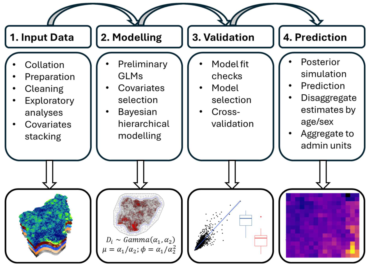
Figure 2.
Spatial distribution of the input demographic datasets. (a) Map of Nigeria showing the nine States where enumeration data from the NMEP anti-malaria bednet campaigns were available. Geolocated household population counts were aggregated to ward levels: b) raw observations – ‘Base’ (c) unrealistic pixel summary values substituted with imputed values – ‘Imputed’ (d) entire wards with unrealistic summary values excluded from the sample – ‘Dropped’.
Figure 2.
Spatial distribution of the input demographic datasets. (a) Map of Nigeria showing the nine States where enumeration data from the NMEP anti-malaria bednet campaigns were available. Geolocated household population counts were aggregated to ward levels: b) raw observations – ‘Base’ (c) unrealistic pixel summary values substituted with imputed values – ‘Imputed’ (d) entire wards with unrealistic summary values excluded from the sample – ‘Dropped’.
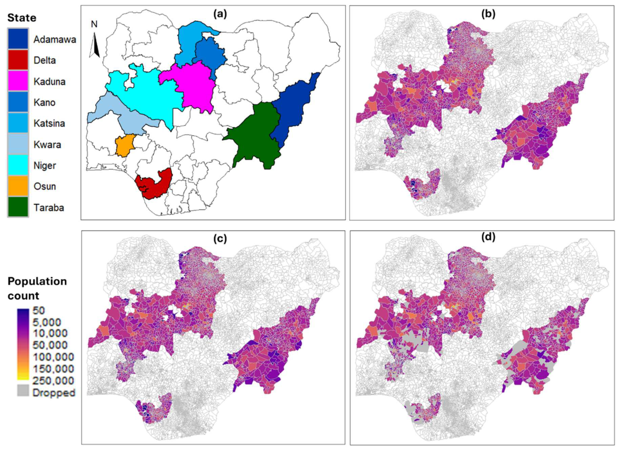
Figure 3.
Model fit metric values from the simulation study for different magnitudes of bias (size of bias), proportion of biased population, and proportion of missing samples (missing prop) across the three methods—Base, Imputed, and Dropped. (a) Mean absolute error (MAE), and (b) Pearson correlation coefficient (CC). The Dropped cleaning approach provided the overall best fit, with the lowest MAE and highest CC values across the majority of data quality scenarios.
Figure 3.
Model fit metric values from the simulation study for different magnitudes of bias (size of bias), proportion of biased population, and proportion of missing samples (missing prop) across the three methods—Base, Imputed, and Dropped. (a) Mean absolute error (MAE), and (b) Pearson correlation coefficient (CC). The Dropped cleaning approach provided the overall best fit, with the lowest MAE and highest CC values across the majority of data quality scenarios.
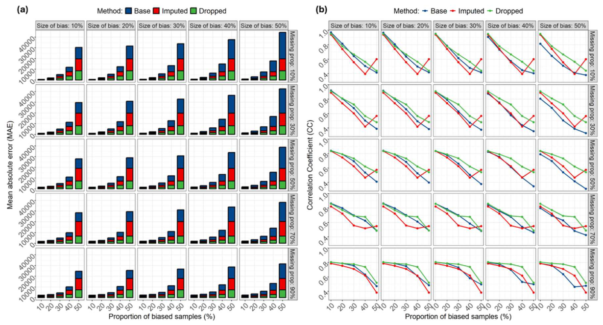
Figure 4.
Cross-validated model fit metrics at the ward level across the three data treatment strategies. (a) Scatterplots of observed versus predicted population counts; (b) Mean absolute error (MAE); (c) Root mean square error (RMSE); (d) Pearson’s correlation coefficient (CC). The Dropped strategy consistently provided the most accurate estimates, with the highest correlation between observed and predicted counts.
Figure 4.
Cross-validated model fit metrics at the ward level across the three data treatment strategies. (a) Scatterplots of observed versus predicted population counts; (b) Mean absolute error (MAE); (c) Root mean square error (RMSE); (d) Pearson’s correlation coefficient (CC). The Dropped strategy consistently provided the most accurate estimates, with the highest correlation between observed and predicted counts.
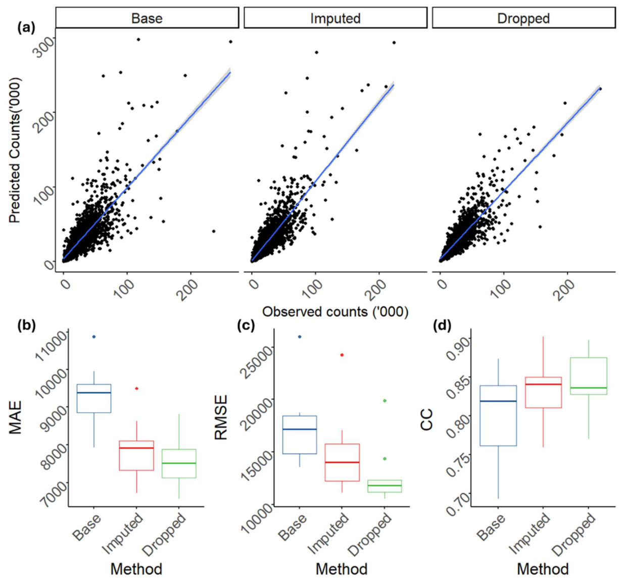
Figure 5.
Spatial distribution of gridded population estimates and aggregated total counts for administrative units in Nigeria at 100 m spatial resolution for 2023/2024. (a) Posterior population counts predicted for each grid cell, with inset maps; (b) Coefficient of variation (CV) of the estimated population counts; (c) Population counts across the wards; (d) Coefficient of variation across the wards; (e) Population counts across the local government areas; (f) Coefficient of variation across the local government areas; (g) Population counts across the states; and (h) Coefficient of variation across the states.Specifically, the highest population estimates were generally observed in LGAs containing the state capital or the main commercial city. For example, in Abia State, the highest population estimates were obtained in Osisioma Ngwa, Obi Ngwa, Umuahia North, Aba North, and Aba South LGAs. Similarly, population estimates were highest in Kano and Port Harcourt LGAs of Kano and Rivers States, respectively.
Figure 5.
Spatial distribution of gridded population estimates and aggregated total counts for administrative units in Nigeria at 100 m spatial resolution for 2023/2024. (a) Posterior population counts predicted for each grid cell, with inset maps; (b) Coefficient of variation (CV) of the estimated population counts; (c) Population counts across the wards; (d) Coefficient of variation across the wards; (e) Population counts across the local government areas; (f) Coefficient of variation across the local government areas; (g) Population counts across the states; and (h) Coefficient of variation across the states.Specifically, the highest population estimates were generally observed in LGAs containing the state capital or the main commercial city. For example, in Abia State, the highest population estimates were obtained in Osisioma Ngwa, Obi Ngwa, Umuahia North, Aba North, and Aba South LGAs. Similarly, population estimates were highest in Kano and Port Harcourt LGAs of Kano and Rivers States, respectively.
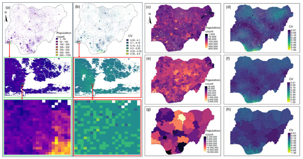

Table 1.
Posterior fixed effects estimates.
| Method | Factor | Mean | SD | 2.5% Quantile | 97.5% Quantile |
|---|---|---|---|---|---|
| Intercept | 1.3576 | 0.0756 | 1.2072 | 1.5061 | |
| Cov1 | 0.0088 | 0.0201 | -0.0307 | 0.0482 | |
| Cov2 | 0.153 | 0.018 | 0.1178 | 0.1882 | |
| Base | Cov3 | 0.1554 | 0.0927 | -0.0246 | 0.3404 |
| Cov4 | -0.0148 | 0.0296 | -0.0726 | 0.0435 | |
| Cov5 | -0.2047 | 0.079 | -0.3597 | -0.0479 | |
| Cov6 | -0.1391 | 0.0094 | -0.1575 | -0.1207 | |
| Intercept | 1.2357 | 0.0679 | 1.1001 | 1.3684 | |
| Cov1 | -0.0015 | 0.0195 | -0.0398 | 0.0369 | |
| Cov2 | 0.1344 | 0.0173 | 0.1005 | 0.1683 | |
| Imputed | Cov3 | 0.0699 | 0.086 | -0.0967 | 0.242 |
| Cov4 | -0.0303 | 0.0282 | -0.0852 | 0.0252 | |
| Cov5 | -0.2507 | 0.0721 | -0.3923 | -0.1077 | |
| Cov6 | -0.1158 | 0.0089 | -0.1333 | -0.0983 | |
| Intercept | 1.1956 | 0.0682 | 1.0595 | 1.3295 | |
| Cov1 | 0.0231 | 0.0177 | -0.0116 | 0.0577 | |
| Cov2 | 0.0859 | 0.016 | 0.0546 | 0.1173 | |
| Dropped | Cov3 | 0.0485 | 0.0878 | -0.1236 | 0.2224 |
| Cov4 | -0.0873 | 0.0257 | -0.1377 | -0.0369 | |
| Cov5 | -0.1833 | 0.0709 | -0.3233 | -0.0432 | |
| Cov6 | -0.0756 | 0.0083 | -0.0919 | -0.0592 |
Note: cov1 – distance to cropland and natural vegetation; cov2 – distance to tree cover; cov3 – annual average precipitation; cov4 – annual average temperature; cov5 – distance to the edges of nature reserves and wilderness areas; and cov6 – evolution of settlement. See Table S1 of the Supplementary Information for further details on the covariates.
Disclaimer/Publisher’s Note: The statements, opinions and data contained in all publications are solely those of the individual author(s) and contributor(s) and not of MDPI and/or the editor(s). MDPI and/or the editor(s) disclaim responsibility for any injury to people or property resulting from any ideas, methods, instructions or products referred to in the content. |
© 2026 by the authors. Licensee MDPI, Basel, Switzerland. This article is an open access article distributed under the terms and conditions of the Creative Commons Attribution (CC BY) license (http://creativecommons.org/licenses/by/4.0/).
Copyright: This open access article is published under a Creative Commons CC BY 4.0 license, which permit the free download, distribution, and reuse, provided that the author and preprint are cited in any reuse.