

Submitted:
28 July 2026
Posted:
31 July 2026
You are already at the latest version
Abstract
Early and accurate classification of melanoma is essential for improving patient outcomes and supporting clinical decision-making. Although numerous predictive models have been proposed, comparisons between classical statistical approaches and modern machine learning algorithms are often limited by heterogeneous analytical workflows and inconsistent validation strategies. This study aimed to compare the predictive performance of classical statistical and machine learning models for melanoma classification using a fully reproducible analytical framework. A retrospective observational study was conducted using the publicly available BCN20000 dermoscopic dataset from the ISIC Archive [1,2]. After standardized data preprocessing, four routinely available clinical variables (age, sex, anatomical site and melanocytic status) were used to develop Logistic Regression, Generalized Additive Models, Random Forest and Extreme Gradient Boosting (XGBoost) classifiers. All models were trained and evaluated using the same stratified training/testing split and their performance was assessed through discrimination, calibration and SHAP explainability analysis. Machine learning models, particularly XGBoost and Random Forest, achieved superior predictive performance compared with conventional statistical approaches, while patient age emerged as the most influential predictor of malignancy. The proposed framework provides a transparent and reproducible approach for objectively comparing predictive models and supports the development of accurate, interpretable and reproducible clinical decision-support systems for melanoma classification.
Keywords:
melanoma classification
; machine learning
; explainable artificial intelligence
; SHAP
; XGBoost
; model calibration
; clinical metadata
; skin lesion diagnosis
1. Introduction
Melanoma is the most aggressive form of skin cancer and is responsible for the majority of skin cancer-related deaths despite accounting for only a small proportion of all skin malignancies. It arises from melanocytes, the pigment-producing cells primarily located in the basal layer of the epidermis, although these cells are also present in mucosal tissue and ocular structures, allowing melanoma to develop in both cutaneous and extra-cutaneous [3].
Early diagnosis is essential because prognosis is strongly associated with disease stage at presentation and tumor thickness. Among the established prognostic factors, Breslow thickness remains the strongest predictor of patient survival and plays a central role in clinical decision-making [3,4].
Cutaneous melanoma comprises several clinico-pathological subtypes that differ in growth pattern and biological behavior, with nodular melanoma generally exhibiting the most aggressive clinical course [3]. Melanoma is uncommon before puberty and occurs predominantly in adults between 30 and 60 years of age.
Over recent decades, melanoma incidence has increased steadily worldwide, making it one of the fastest-growing malignancies in terms of incidence. According to the latest GLOBOCAN 2022 estimates, approximately 331,700 new melanoma cases and 58,700 melanoma-related deaths occurred worldwide, ranking melanoma as the seventeenth most common cancer globally. The highest incidence rates are observed in countries with predominantly fair-skinned populations exposed to high levels of solar ultraviolet radiation, such as Australia and several Northern European countries [5,6]. In Italy, melanoma represents an increasingly important public health challenge. According to the latest national estimates, approximately 13,000 new melanoma cases are diagnosed annually, highlighting the growing burden of the disease on the national healthcare system [7]. Over the last decades, melanoma incidence has shown a steady increase, whereas mortality has remained relatively stable, largely reflecting earlier diagnosis and substantial advances in therapeutic strategies. Moreover, marked geographical differences have been reported across the country, with generally higher incidence rates in Northern than in Southern Italy, likely reflecting differences in skin phenotype, behavioral habits and cumulative ultraviolet radiation exposure [8].
The increasing burden of melanoma, together with the substantial survival advantages associated with early diagnosis, has stimulated growing interest in computer-assisted diagnostic systems (CADS) and predictive models capable of supporting clinicians during diagnostic assessment. Advances in statistical learning and artificial intelligence (AI) have enabled the development of increasingly sophisticated predictive models for melanoma classification, ranging from conventional statistical approaches to modern machine learning and deep learning algorithms. These methods have demonstrated considerable potential for improving diagnostic accuracy and supporting clinical decision-making.
However, despite the large number of predictive models proposed in the literature, direct comparisons between different analytical approaches remain challenging. Existing studies frequently employ heterogeneous datasets, different predictor variables, variable pre-processing pipelines, inconsistent validation strategies and diverse performance metrics, making it difficult to objectively assess the relative strengths and limitations of individual algorithms. Furthermore, while many investigations primarily focus on maximizing predictive performance, considerably less attention has been devoted to model calibration, clinical utility and explainability, all of which are essential prerequisites for the safe implementation of artificial intelligence in clinical practice.
These limitations highlight the need for standardized and reproducible analytical frameworks capable of objectively comparing predictive models while ensuring predictive accuracy, clinical interpretability and reproducibility. To address this gap, the present study presents a systematic comparison of conventional statistical models and state-of-the-art machine learning algorithms for melanoma classification using routinely collected clinical variables from a publicly available dataset. The evaluated models were compared in terms of discrimination, calibration, explainability, clinical utility, thereby providing a 76 comprehensive assessment of the different modeling approaches.
Over the past decade, artificial intelligence has profoundly transformed melanoma diagnosis, leading to the development of numerous predictive models based on statistical learning, machine learning and deep learning techniques. A major milestone was represented by the work of Esteva et al., who demonstrated dermatologist-level performance using deep convolutional neural networks trained on large image datasets. Since then, numerous studies have proposed increasingly sophisticated algorithms for melanoma classification using dermoscopic images, structured clinical variables, or multimodal data. Recent systematic reviews consistently report promising diagnostic performance while also highlighting important methodological challenges that continue to limit the translation of these models into routine clinical practice [9,10,11,12].
Conventional statistical approaches, particularly Logistic Regression, have historically represented the reference methodology for developing clinically interpretable prediction models. More recently, machine learning algorithms, including Random Forest, XGBoost, LightGBM and CatBoost, have demonstrated improved predictive performance, especially when trained on large clinical datasets. In parallel, convolutional neural networks and, more recently, transformer-based architectures have become the dominant approaches for dermoscopic image analysis. Several investigations have also explored multimodal frameworks integrating clinical metadata with imaging information, highlighting the potential benefits of combining complementary sources of patient information [13,14,15,16].
Despite these advances, important methodological limitations remain. Existing studies frequently rely on heterogeneous datasets, different predictor variables, inconsistent preprocessing pipelines and diverse validation strategies, which makes direct comparisons between predictive models particularly challenging. Moreover, many investigations primarily focus on discrimination metrics, whereas calibration, explainability, clinical utility and external validation receive considerably less attention despite their importance for clinical implementation. Although multi-modal artificial intelligence has emerged as a promising research direction, the predictive value of routinely collected clinical variables remains comparatively under-explored and standardized analytical frameworks enabling objective comparisons between modeling approaches are still lacking [10,11,17,18].
These considerations provide the rationale for the present study, which systematically compares conventional statistical and machine learning models using a standardized analytical framework based on routinely collected clinical variables.
2. Materials and Methods
This study was designed to systematically compare the performance of classical statistical models and modern machine learning algorithms for the binary classification of melanoma lesions using structured clinical and dermoscopic data. A unified analytical framework was adopted to ensure that all predictive models were developed, validated and evaluated under identical experimental conditions, allowing differences in predictive performance to be attributed solely to the modeling approach rather than to variations in data processing or validation strategies.
The complete analytical workflow consisted of six sequential phases: dataset preparation, data preprocessing, predictive model development, model training and validation, performance evaluation and model interpretation. Throughout the analysis, identical predictor variables, data partitioning strategies and evaluation metrics were employed across all models to guarantee a fair and reproducible comparison.
Four supervised binary classification models were investigated, spanning both traditional statistical learning and modern ensemble machine learning techniques. Logistic Regression was considered as the reference statistical approach, while Generalized Additive Models were included to account for potential nonlinear effects without sacrificing interpretability. Random Forest and Extreme Gradient Boosting were subsequently evaluated as representative ensemble learning algorithms capable of modeling increasingly complex relationships among predictors.
The following sections describe each phase of the analytical pipeline, including data preprocessing, the theoretical foundations of the evaluated predictive models, the model development strategy and the statistical procedures adopted to assess discrimination, calibration and clinical utility.
2.1. Data Pre-Processing
Prior to the statistical analyses and predictive modeling, the dataset underwent a standardized pre-processing procedure to ensure data quality, consistency and reproducibility. The data-handling workflow included data inspection, verification of variable consistency, identification of duplicate records, management of missing or non-informative values, harmonization of categorical variables and preparation of the outcome variable for subsequent analyses.
Categorical predictors were encoded according to the requirements of the different statistical and machine learning models, while continuous variables were retained in their original numerical format whenever appropriate. The outcome variable was subsequently reformulated as a binary classification problem by considering only lesions with a definitive benign or malignant diagnosis.
Finally, the processed dataset was partitioned into independent training and testing subsets using stratified random sampling in order to preserve the class distribution across both sets. The same data partition was employed for all evaluated models, ensuring a fair and reproducible comparison of predictive performance.
A detailed description of the statistical and machine learning models employed in this study is provided in the following subsection.
2.2. Logistic Regression—LR
The first employed model is the Logistic regression [19]. LR is a supervised statistical model widely used for binary classification problems. In this study, it was employed to estimate the probability that a skin lesion belongs to the malignant class on the basis of the available clinical and dermoscopic predictors. Logistic Regression was selected as the baseline model because of its interpretability, its established use in clinical prediction research and its ability to provide individual probabilities rather than only class labels.
Let Yi denote the outcome observed for the i-th lesion, defined as
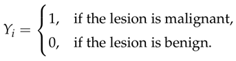
For each lesion, let

represent the vector of p predictor variables. The objective of LR is to estimate the conditional probability

that is, the probability that the i-th lesion is malignant given its observed characteristics.
Because probabilities must lie between 0 and 1, Logistic Regression does not model pi directly as a linear function of the predictors. Instead, it models the logarithm of the odds of malignancy through the logit link function:
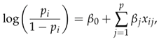
where β0 is the intercept and βj is the coefficient associated with the j-th predictor.
The corresponding estimated probability of malignancy is obtained through the inverse-logit transformation:
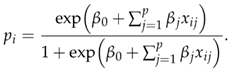
Equivalently, the same expression can be written as
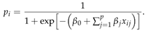
The regression coefficients are estimated by Maximum Likelihood Estimation (MLE). For independent observations, the likelihood function is:
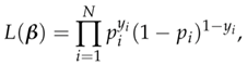
where N is the total number of observations. The estimated coefficient vector βs is the one that maximizes the probability of observing the outcomes available in the training dataset. An important advantage of Logistic Regression is the direct interpretability of its coefficients. For a continuous predictor xj, the quantity
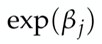
represents the odds ratio associated with a one-unit increase in that predictor, holding the remaining variables constant. Values greater than 1 indicate increased odds of malignancy, whereas values lower than 1 indicate decreased odds. For categorical predictors, the odds ratio compares a given category with the selected reference category.
In the present analysis, Logistic Regression served two main purposes. First, it provided an interpretable estimate of the association between each predictor and the probability of melanoma. Second, it represented the reference model against which the predictive performance of the more flexible approaches was compared. Once an estimated probability was obtained, lesions could be assigned to the benign or malignant class according to a decision threshold c:
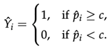
Although a threshold of 0.5 is commonly used, the optimal threshold may depend on the clinical objective. In melanoma classification, for example, greater emphasis may be placed on sensitivity in order to reduce the number of malignant lesions incorrectly classified as benign.
Despite its interpretability, Logistic Regression assumes that continuous predictors have a linear relationship with the log-odds of the outcome. It also does not automatically identify nonlinear effects or interactions among predictors. These limitations justify the comparison with Generalized Additive Models and tree-based machine learning algorithms.
2.3. Generalized Additive Models—GAMs
GAMs extend the Generalized Linear Model [20] framework by relaxing the assumption that continuous predictors are linearly related to the log-odds of the outcome. Instead of estimating a single regression coefficient for each continuous predictor, GAMs model their effects through smooth functions that are estimated directly from the data.
For a binary classification problem, the model can be written as
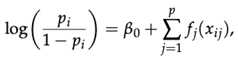
where pi denotes the probability that the i-th lesion is malignant, β0 is the intercept and fj(·) represents a smooth function describing the effect of the j-th predictor. In practice, these smooth functions are commonly approximated using penalized regression splines, whose degree of smoothness is automatically determined during model fitting.
Compared with Logistic Regression, GAMs retain the probabilistic interpretation of the model while allowing nonlinear relationships between continuous predictors and the outcome to be captured without specifying their functional form a-priori. This characteristic is particularly relevant when the association between clinical variables and melanoma risk is expected to deviate from linearity.
Although GAMs substantially increase modeling flexibility, they preserve an additive structure and therefore do not automatically account for complex interactions among predictors. For this reason, more flexible non-parametric approaches, such as Random Forest, were also evaluated in this study.
2.4. Random Forest—RF
In the framework of supervised ensemble learning there is the well-known Random Forest [21] that combines multiple decision trees to improve predictive performance and reduce overfitting. Unlike Logistic Regression and GAMs, which require the relationship between predictors and the outcome to be specified through a predefined functional form, Random Forest is a non-parametric method that automatically learns nonlinear relationships and complex interactions directly from the data.
The algorithm is based on the principle of bootstrap aggregating (bagging). Multiple bootstrap samples are generated from the original training dataset and an independent decision tree is fitted to each sample. During tree construction, only a random subset of predictors is considered at each node, increasing tree diversity and reducing the correlation among individual models.
For a binary classification problem, the final prediction is obtained by aggregating the predictions of all trees through majority voting,

where Tb(x) denotes the prediction of the b-th decision tree and B is the total number of trees in the ensemble.
The combination of bootstrap sampling and random feature selection enables Random Forest to achieve robust predictive performance while effectively modeling nonlinear effects and higher-order interactions among predictors. Furthermore, the algorithm provides estimates of variable importance, allowing the relative contribution of each predictor to the classification task to be assessed.
Although Random Forest generally exhibits excellent predictive accuracy and robustness, all trees are constructed independently and contribute equally to the final prediction. This limitation motivated the development of boosting algorithms, such as XGBoost, which iteratively build decision trees by focusing on the prediction errors made by the current ensemble.
2.5. Extreme Gradient Boosting (XGBoost)
Extreme Gradient Boosting (XGBoost) [22] is a supervised ensemble learning algorithm based on the gradient boosting framework. Unlike Random Forest, where decision trees are constructed independently and their predictions are combined through majority voting, XGBoost builds trees sequentially. Each new tree is trained to reduce the prediction errors made by the existing ensemble, progressively improving the overall predictive 259 performance.
For an input observation xi, the prediction after K boosting iterations is expressed as
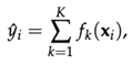
where fk(·) represents the decision tree added at the k-th iteration. At each boosting step, the algorithm optimizes a regularized objective function of the form
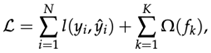
where l(·) is the loss function measuring the discrepancy between observed and predicted outcomes and Ω(·) is a regularization term that penalizes model complexity. This regularization reduces the risk of overfitting while maintaining high predictive accuracy. During model training, XGBoost exploits first- and second-order gradient information to efficiently determine how each newly generated tree should minimize the remaining prediction errors. Additional optimization strategies, including shrinkage (learning rate), row and column subsampling and tree pruning, further improve model generalization and computational efficiency.
Compared with Random Forest, XGBoost generally provides greater predictive accuracy by iteratively refining the ensemble instead of constructing trees independently. This flexibility allows the algorithm to effectively capture complex nonlinear relationships and interactions among predictors, making it one of the most widely adopted machine learning methods for structured tabular data.
In the present study, XGBoost represented the most flexible predictive model included in the comparative analysis. Its predictive performance was evaluated against Logistic Regression, Generalized Additive Models and Random Forest under an identical training and validation framework to investigate whether the additional modeling complexity translated into improved melanoma classification. Despite its excellent predictive performance, XGBoost is generally regarded as a black-box model because the contribution of individual predictors to the final prediction cannot be directly inferred from the fitted ensemble of decision trees. This limited interpretability may hinder its adoption in clinical settings, where understanding the rationale underlying a prediction is often as important as the prediction itself. To address this limitation, post-hoc model interpretation techniques have been developed to provide insight into the behavior of complex machine learning models.
2.6. SHapley Additive exPlanations—SHAP
To improve the interpretability of the best-performing machine learning model, SHapley Additive exPlanations [23,24] were employed. SHAP is a post-hoc explainability framework based on cooperative game theory that quantifies the contribution of each predictor to an individual model prediction.
For a given observation, SHAP decomposes the predicted outcome into the sum of the contributions of all predictor variables relative to a baseline prediction. Formally, the prediction can be expressed as
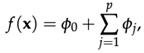
where φ0 represents the baseline prediction of the model and φj denotes the SHAP value associated with the j-th predictor. Positive SHAP values increase the predicted probability of melanoma, whereas negative values decrease it.
Unlike traditional feature importance measures, SHAP provides both global and local model explanations. Global interpretation identifies the variables that most strongly influence the overall predictive behavior of the model, whereas local interpretation explains how each predictor contributes to the prediction of an individual patient.
In this study, SHAP analysis was performed on the best-performing predictive model. Global feature importance was assessed using mean absolute SHAP values and bees-warm plots, while dependence plots were used to investigate how changes in individual predictors influenced the predicted probability of melanoma.
3. Results
This section presents the results of the descriptive, inferential and predictive analyses. The findings are organized according to the analytical workflow, beginning with the description of the study population and followed by the evaluation of the statistical and machine learning models, including their discrimination, calibration and explainability.
3.1. Study Population
The original BCN20000 dataset comprised 18,946 skin lesions. After excluding lesions without a definitive diagnosis, 17,790 observations remained available for the descriptive analyses. Of these, 7,831 (44.0%) were classified as benign, 1,088 (6.1%) as indeterminate and 8,871 (49.9%) as malignant.
The distribution of lesions according to the final diagnostic category is shown in Figure 1. As illustrated, benign and malignant lesions accounted for the large majority of the study population, occurring in comparable proportions, whereas indeterminate lesions represented only a minor fraction of the overall sample.
Patient age differed markedly across the three diagnostic categories. As shown in Figure 2, benign lesions were predominantly observed in younger individuals (median 45 years, IQR: 35–65), whereas malignant lesions occurred mainly in older patients (median 65 years, IQR: 50–75). Indeterminate lesions exhibited the highest median age (70 years, IQR: 60–80).
The age distributions showed a progressive shift towards older ages from benign to malignant lesions, although partial overlap between the three diagnostic groups was 331 observed.
Lesion location showed substantial variability across the diagnostic categories, as illustrated in Figure 3. Benign lesions were predominantly located on the anterior torso (49.4%), followed by the lower extremities (16.4%) and the head and neck region (15.6%). In contrast, malignant lesions exhibited a more heterogeneous anatomical distribution, with the anterior torso (36.4%) and the head and neck region (27.7%) representing the most frequently affected sites. Indeterminate lesions displayed a markedly different pattern, 338 with nearly three-quarters of cases (74.1%) located in the head and neck region.
Melanocytic status also differed substantially across the diagnostic categories, as shown in Figure 4. Most benign lesions were classified as melanocytic (72.1%), whereas malignant lesions showed a more balanced distribution between melanocytic (52.3%) and non-melanocytic (47.7%) lesions. All indeterminate lesions were classified as non-melanocytic.
The demographic and clinical characteristics of lesions with a definitive diagnosis are summarized in Table 1. The table provides an overall comparison of the three diagnostic groups across the main variables considered in this study, complementing the graphical representations presented in Figure 1, Figure 2, Figure 3 and Figure 4.
Overall, the descriptive analyses showed differences among the three diagnostic groups with respect to age, sex, anatomical site and melanocytic status. These findings were subsequently evaluated using inferential statistical methods.
3.2. Inferential Analysis
The differences observed in the descriptive analyses were formally assessed using inferential statistical methods. The Kruskal–Wallis test identified significant differences in age among the three diagnostic groups (p < 0.001). Likewise, Pearson’s chi-squared tests revealed statistically significant associations between diagnostic category and all investigated categorical variables, including sex, anatomical site and melanocytic status (all p < 0.001).
The assumptions underlying the chi-squared analyses were verified by inspecting the expected cell frequencies of the contingency tables. Only one expected frequency was below five, corresponding to 5.56% of the total expected cell counts, thereby satisfying the conventional assumptions for the validity of Pearson’s chi-squared test.
Overall, the inferential analyses confirmed that the three diagnostic groups differed significantly across all investigated demographic and clinical characteristics.
3.3. Predictive Modelling
Following the descriptive and inferential analyses, predictive modeling was performed using the subset of lesions with a definitive benign or malignant diagnosis. Indeterminate lesions were excluded from model development in order to formulate a binary classification problem. The final modeling dataset consisted of 16,358 lesions, which were randomly partitioned into a training cohort (13,087 observations) and an independent testing cohort (3,271 observations). The predictive performance of four classification models was subsequently evaluated on the independent testing cohort using identical validation procedures.
3.3.1. Logistic Regression
Logistic Regression was adopted as the baseline statistical model for binary classification. The model achieved an area under the receiver operating characteristic curve (AUC) of 0.731 (95% CI: 0.714–0.748).
The model achieved an overall accuracy of 67.3% on the independent testing cohort. Sensitivity and specificity were 70.4% and 63.8%, respectively. The corresponding positive and negative predictive values were 68.8% and 65.5%, respectively, resulting in an F1-score of 0.696. The Brier score was 0.208.
3.3.2. Generalized Additive Model
The Generalized Additive Model (GAM) extended the Logistic Regression framework by allowing nonlinear effects of age while retaining the remaining predictors as parametric terms. The model achieved an area under the receiver operating characteristic curve (AUC) of 0.733 (95% CI: 0.716–0.750).
The model achieved an overall accuracy of 67.8%. Sensitivity and specificity were 72.6% and 62.3%, respectively. The corresponding positive and negative predictive values were 68.6% and 66.7%, respectively, resulting in an F1-score of 0.705. The Brier score was 0.207.
3.3.3. Random Forest
The Random Forest classifier achieved an area under the receiver operating characteristic curve (AUC) of 0.756 (95% CI: 0.740–0.773).
The model achieved an overall accuracy of 70.7%, together with a balanced accuracy of 70.4%. Sensitivity and specificity were 76.4% and 64.4%, respectively. The corresponding positive and negative predictive values were 70.9% and 70.6%, respectively, resulting in an F1-score of 0.735. The Brier score was 0.243.
3.3.4. Extreme Gradient Boosting
The Extreme Gradient Boosting (XGBoost) classifier achieved an area under the receiver operating characteristic curve (AUC) of 0.768 (95% CI: 0.752–0.784).
The model achieved an overall accuracy of 69.8%. Sensitivity and specificity were 77.1% and 61.6%, respectively. The corresponding positive and negative predictive values were 68.6% and 71.4%, respectively, resulting in an F1-score of 0.731. The Brier score was 0.194.
The predictive performance of all evaluated models is summarized in Table 2. While these metrics reflect model performance at a single, predefined decision threshold, Receiver Operating Characteristic (ROC) curves and the corresponding Areas Under the Curve (AUCs) allow the discriminative performance of the four classification models to be assessed independently of the selected threshold [25]. The ROC curves of the four evaluated models are presented in Figure 5.
As shown in Figure 5, XGBoost achieved the highest AUC (0.768), followed by Random Forest (0.756). Logistic Regression and the Generalized Additive Model achieved AUCs of 0.731 and 0.733, respectively.
To assess whether the observed differences in discriminative performance were statistically significant, pairwise comparisons of the AUCs were performed using DeLong’s nonparametric test [26]. The results are reported in Table 3
A calibration plot depicts the agreement between predicted probabilities and observed outcome frequencies, by plotting predicted probabilities (x-axis) against observed probabilities (y-axis), typically grouped into bins or smoothed across the probability range. A model is considered well calibrated when the resulting curve closely follows the diagonal line of identity (y = x), indicating that predicted probabilities correspond to the actual observed frequencies of the outcome.
Calibration of the predicted probabilities was evaluated using calibration plots. The calibration plots of the four evaluated classification models are presented in Figure 6.
As shown in Figure 6, differences in calibration were observed across the evaluated models. The XGBoost model showed calibration estimates that remained closest to the reference diagonal over most of the predicted probability range. Logistic Regression and the Generalized Additive Model exhibited similar calibration patterns, whereas Random Forest showed larger deviations from the reference line, particularly at higher predicted probabilities.
3.4. Model Interpretability
Given that XGBoost achieved the highest AUC and the lowest Brier score among the evaluated models, its predictions were further investigated using SHapley Additive exPlanations (SHAP). SHAP values quantify the contribution of each predictor to the model output, allowing both the overall importance of the included variables and the direction of their effects on the predicted probability of malignancy to be assessed.
The global behavior of the model was first evaluated using a SHAP summary (bees-warm) plot, whereas the relationship between age and the corresponding SHAP values was subsequently examined using a SHAP dependence plot.
As shown in Figure 7, the predictor age exhibited the largest distribution of SHAP values and ranked as the most influential predictor in the XGBoost model. Melanocytic status was the second most influential variable, followed by anatomical site and sex. Higher age values were generally associated with positive SHAP values, whereas lower age values were associated with negative SHAP values.
To further examine the contribution of the most influential predictor, a SHAP dependence plot was generated for age.
Figure 8 shows that SHAP values generally increased with age. Younger individuals were predominantly associated with negative SHAP values, whereas older individuals were associated with positive SHAP values. A transition from predominantly negative to predominantly positive SHAP values was observed around 55 years of age.
4. Discussion
The results presented in the previous section provide a comprehensive overview of the predictive performance achieved by conventional statistical models and modern machine learning algorithms for melanoma classification using routinely available clinical metadata. Although all evaluated approaches demonstrated acceptable discriminative ability, meaningful differences emerged in terms of discrimination, probability calibration and model interpretability. Rather than simply identifying the algorithm associated with the highest predictive performance, the present comparison allows a broader interpretation of the relative strengths and limitations of each modeling strategy when applied to structured clinical data.
The ensemble learning approaches outperformed the regression-based models across most performance metrics. XGBoost achieved the highest discriminative ability (AUC 0.768, 95% CI: 0.752–0.784) and the lowest Brier score (0.194), whereas Random Forest provided the highest overall classification accuracy (70.7%) and sensitivity (76.4%), albeit at the cost of the poorest calibration among the four models (Brier score 0.243). Logistic Regression and the GAM achieved comparable, more modest discrimination (AUC 0.731 and 0.733, respectively) and accuracy (67.3% and 67.8%, respectively). Pairwise DeLong comparisons confirmed that these differences in discrimination were statistically significant, indicating that the observed advantage of the ensemble methods and of XGBoost in particular, was unlikely to be attributable to chance. However, statistical significance in a dataset of this size does not necessarily imply clinical relevance: an AUC difference of three to four percentage points, while unlikely to arise by chance, may translate into only marginal differences in individual-level risk stratification and should therefore be weighed against practical considerations such as interpretability and computational cost when selecting a model for clinical use.
This pattern of moderate, though statistically significant, improvement is informative in itself. It suggests that the ceiling on predictive performance in this setting is set less by the algorithm’s capacity to model complexity and more by the informativeness of the input variables. Age, anatomical site, melanocytic status and sex jointly capture epidemiological risk but do not encode the morphological and textural cues (asymmetry, border irregularity, color heterogeneity, dermoscopic structures) that clinicians rely on for visual diagnosis. The fact that even a flexible, interaction-capturing algorithm such as XGBoost could not substantially exceed the performance of Logistic Regression indicates that this ceiling reflects a genuine information limit in the predictor set, rather than an inability of the simpler models to exploit the available data. This observation reframes the comparison: the central finding is not that one algorithm is superior in absolute terms, but that algorithmic choice matters comparatively little once the informational content of routinely collected metadata has been exhausted.
This observation is particularly relevant because the present study intentionally excluded dermoscopic images and focused exclusively on structured clinical variables routinely collected during clinical assessment. Consequently, the obtained results should not be interpreted as the maximum predictive performance achievable for melanoma classification, but rather as an estimate of the information that can be extracted from patient metadata alone. Unlike previous investigations primarily focused on dermoscopic images or multimodal artificial intelligence systems, the present study deliberately restricted the analysis to routinely available structured clinical metadata, allowing the predictive contribution of demographic and clinical characteristics to be evaluated independently of image-derived information. Framed this way, the present findings can be regarded as a lower-bound, image-independent benchmark against which the incremental value of dermoscopic or multimodal information can be quantified in future work, rather than as a standalone diagnostic proposal.
The observed superiority of the ensemble learning methods is consistent with the general trend reported in the recent literature on melanoma prediction. Over the last-decade, several studies have shown that machine learning algorithms are capable of exploiting complex interactions among predictors more effectively than conventional statistical models, often leading to improvements in predictive performance. Nevertheless, the magnitude of these improvements has varied considerably across studies, largely because of differences in study populations, predictor selection, validation strategies and outcome definitions, which limits direct numerical comparison with the present results and supports interpreting the observed AUC values in relative rather than absolute terms.
The different behavior observed across the evaluated models can be interpreted in light of their underlying statistical assumptions. Logistic Regression represents the most parsimonious approach among the evaluated classifiers and assumes a linear relationship between the predictors and the log-odds of the outcome. The GAM partially relaxed this assumption by introducing a nonlinear smooth function for age while maintaining the remaining predictors as parametric terms; despite this additional flexibility, only marginal improvements in AUC (0.733 versus 0.731) and Brier score (0.207 versus 0.208) were observed, suggesting that the relationship between age and malignancy risk, although clinically graded rather than strictly linear, is captured reasonably well even by a linear log-odds term and that most of the unexplained variance lies elsewhere, plausibly in unmeasured lesion-level characteristics rather than in the functional form of age alone. Conversely, the ensemble learning methods were able to capture complex nonlinear relationships and higher-order interactions among the available predictors without requiring explicit model specification. Random Forest achieved the highest overall classification accuracy, whereas XGBoost consistently provided the best discrimination and probability calibration, consistent with the theoretical characteristics of boosting algorithms, which iteratively reduce prediction errors by sequentially combining multiple weak learners into a more accurate predictive model and which are typically more robust than bagging-based approaches such as Random Forest when the underlying signal-to-noise ratio is low.
The calibration analysis adds a further, clinically important layer to this interpretation. Although Random Forest achieved higher raw classification accuracy than XGBoost, its calibration plot showed larger deviations from the reference diagonal, particularly at higher predicted probabilities and its Brier score was the highest among the four models. This combination is a recognized property of bagging-based ensembles, which tend to average away extreme predictions and can therefore under- or over-estimate risk at the tails of the probability distribution even while preserving good rank-ordering of cases. In a clinical setting, this distinction matters: a model used to prioritize patients for further investigation depends primarily on discrimination, whereas a model used to communicate individual risk, for instance to support a decision on biopsy or referral, depends critically on calibration, since a poorly calibrated “80% probability of malignancy” may not correspond to an actual 80% observed frequency of malignancy. Because probability calibration is particularly relevant whenever predicted probabilities are intended to inform clinical decision-making rather than merely to rank patients, the consistently good calibration of XGBoost across most of the predicted probability range, together with its superior discrimination and lowest Brier score, supports its selection as the primary model for further interpretation and, potentially, for downstream clinical application.
Taken together, these findings suggest that, within the context of structured clinical metadata, the predictive information available in the selected variables may represent the principal limiting factor on model performance. Consequently, future improvements are likely to depend not only on increasingly sophisticated machine learning algorithms but also on the integration of additional clinically informative predictors capable of capturing the biological complexity of melanoma.
Given its superior discrimination, calibration and Brier score, the XGBoost model was further investigated using SHAP analysis in order to characterize the contribution of individual predictors to its output. Among the evaluated predictors, age emerged as the dominant contributor, followed by melanocytic status, anatomical site and sex. This ranking is consistent with the descriptive and inferential analyses presented in the previous sections, which identified statistically significant differences in age, anatomical site and melanocytic status across diagnostic groups and reflects well-established epidemiological evidence indicating that melanoma incidence increases substantially with advancing age, most plausibly as a consequence of cumulative ultraviolet exposure and age-related accumulation of somatic mutations in melanocytes.
Beyond feature ranking, the SHAP dependence analysis demonstrated that increasing age was consistently associated with higher predicted probabilities of malignancy, whereas younger age contributed negatively to the model output. The transition from predominantly negative to predominantly positive SHAP values observed around 55 years of age further suggests the presence of a gradual increase in predicted melanoma risk rather than an abrupt threshold effect, which is biologically more plausible than a discrete cut-off and is consistent with the descriptive comparison of median age across diagnostic categories, in which malignant lesions occurred mainly in older patients (median 65 years) than benign lesions (median 45 years). Rather than functioning as an arbitrary diagnostic cut-off, this transition may be more usefully interpreted as identifying an age range around which clinical vigilance could reasonably be increased, complementing rather than replacing morphological assessment.
From a clinical perspective, the availability of local explanation methods represents an important advantage over many conventional “black-box” artificial intelligence systems. The possibility of identifying the variables driving each individual prediction may increase model transparency, facilitate clinician confidence and support the future integration of machine learning algorithms into routine dermatological decision-making. In particular, a model whose predictions can be traced back to established epidemiological risk factors, such as age, anatomical site and melanocytic status, is more likely to be trusted and scrutinized effectively by clinicians than one whose reasoning cannot be inspected, which is a prerequisite for the safe clinical adoption of any decision-support tool. Consequently, explainability should not be regarded as an additional component of predictive modeling, but rather as an essential requirement for the development of clinically applicable artificial intelligence systems.
5. Conclusions
This study evaluated the ability of conventional statistical methods and modern machine learning algorithms to classify melanoma using routinely available structured clinical metadata, developing all models within a single, consistent analytical framework to enable a rigorous and unbiased comparison of their discrimination, calibration and explainability.
The evaluated machine learning algorithms provided measurable, though moderate, improvements over conventional regression-based approaches. XGBoost achieved the best overall balance of discrimination and calibration, Random Forest achieved the highest classification accuracy at the cost of less reliable probability estimates and both Logistic Regression and the Generalized Additive Model achieved satisfactory performance despite their simpler structure. This pattern indicates that routinely collected clinical metadata already contain substantial predictive information for melanoma classification, largely independent of the specific modeling technique employed and suggests that further gains in predictive performance are more likely to come from richer predictor sets than from increasingly complex algorithms alone.
Beyond the comparison of predictive algorithms, the principal contribution of this work lies in the definition of a transparent, reproducible and statistically rigorous analytical framework for the investigation of structured clinical data. Rather than focusing exclusively on predictive performance, the proposed workflow integrates descriptive and inferential statistical analysis, predictive modeling, calibration assessment, formal statistical comparison of model discrimination and explainable artificial intelligence within a single methodological pipeline. This integration is intended to facilitate reproducibility, improve methodological transparency and provide a reference framework that can be extended to other structured clinical datasets beyond the melanoma classification task addressed here.
6. Future Developments
The present study should be regarded as a predictive stage within a broader research program. The comparison between conventional statistical methods and machine learning algorithms presented in this work allows the classification ability of each model, that is, its capacity to assign lesions to the correct diagnostic class in a manner conceptually related to instance-based approaches such as k-nearest neighbors, but relying on more sophisticated decision rules, to be characterized and interpreted through established quantitative measures, including odds ratios, discrimination metrics such as the AUC, and variable importance. In this sense, the present work provides a rigorous predictive and interpretive baseline, establishing which clinical variables contribute most to melanoma classification and to what extent, before extending the analysis beyond prediction.
As an immediate next step, the analytical pipeline developed in this study will be applied to a real-world Italian dataset collected at the ASST Spedali Civili di Brescia. This will serve a twofold purpose: first, to further validate the proposed methodological framework on an independent, prospectively collected clinical population; second, to compare two geographically distinct but closely related populations, given that the BCN20000 dataset employed in the present study was collected in Barcelona. Such a comparison may help assess the generalizability of the identified predictors and of the models’ performance across different clinical settings and, potentially, different population characteristics.
Beyond this validation stage, future work will move from a purely predictive framework towards the discovery of the latent structure underlying melanoma heterogeneity, analogous to how latent variable models such as Latent Dirichlet Allocation (LDA) uncover hidden thematic structure in textual data. This will be pursued through diagnosis profiling, similarity matrices based on mixed clinical variables computed via Gower distance, network construction and community detection algorithms, and the development of a dermatological atlas. Conceptually related to topic modeling approaches, but applied to the study of melanoma, this methodology is intended to move beyond the assignment of a single predicted diagnostic class and instead uncover clinically meaningful patient subgroups, diagnostic clusters and clinical communities represented as network graphs. Combined with explainable artificial intelligence and dermoscopic knowledge, these approaches may ultimately contribute to the development of next-generation clinical decision-support systems capable not only of predicting melanoma risk, but also of supporting clinicians in interpreting and understanding individual patient profiles within a broader disease atlas.
Acknowledgments
In this section, you can acknowledge any support given that is not covered by the author contribution or funding sections. This may include administrative and technical support, or donations in kind (e.g., materials used for experiments). Where GenAI has been used for purposes such as generating text, data, or graphics, or for study design, data collection, analysis, or interpretation of data, please add “During the preparation of this manuscript/study, the author(s) used [tool name, version information] for the purposes of [description of use]. The authors have reviewed and edited the output and take full responsibility for the content of this publication.”.
Conflicts of Interest
Declare conflicts of interest or state “The authors declare no conflicts of interest.” Authors must identify and declare any personal circumstances or interests that may be perceived as inappropriately influencing the representation or interpretation of reported research results. Any role of the funders in the design of the study; in the collection, analyses or interpretation of data; in the writing of the manuscript; or in the decision to publish the results must be declared in this section. If there is no role, please state “The funders had no role in the design of the study; in the collection, analyses, or interpretation of data; in the writing of the manuscript; or in the decision to publish the results”.:
Abbreviations
The following abbreviations are used in this manuscript:
| MDPI | Multidisciplinary Digital Publishing Institute |
| DOAJ | Directory of open access journals |
| TLA | Three-letter acronym |
| LD | Linear dichroism |
References
- International Skin Imaging Collaboration (ISIC). BCN20000 Collection. 2026. Available online: https://api.isic-archive.com/collections/249/.
- Hernández-Pérez, C.; Combalia, M.; Podlipnik, S.; Codella, N.C.F.; Rotemberg, V.; Halpern, A.C.; Reiter, O.; Carrera, C.; Barreiro, A.; Helba, B.; et al. BCN20000: Dermoscopic Lesions in the Wild. Sci. Data 2024, 11, 641. [Google Scholar] [CrossRef]
- National Comprehensive Cancer Network. NCCN Clinical Practice Guidelines in Oncology: Cutaneous Melanoma. Version 2.2024. J. Natl. Compr. Cancer Netw. 2024, 22, 290–359. [Google Scholar] [CrossRef]
- Gershenwald, J.E.; Scolyer, R.A.; Hess, K.R.; Sondak, V.K.; Long, G.V.; Ross, M.I.; Lazar, A.J.; Faries, M.B.; Kirkwood, J.M.; McArthur, G.A.; et al. Melanoma staging: Evidence-based changes in the American Joint Committee on Cancer eighth edition cancer staging manual. CA A Cancer 658 J. Clin. 2017, 67, 472–492. [Google Scholar] [CrossRef] [PubMed]
- Bray, F.; Laversanne, M.; Sung, H.; Ferlay, J.; Siegel, R.L.; Soerjomataram, I.; Jemal, A. Global cancer statistics 2022: GLOBOCAN estimates of incidence and mortality worldwide for 36 cancers in 185 countries. CA A Cancer J. Clin. 2024, 74, 229–263. [Google Scholar] [CrossRef] [PubMed]
- International Agency for Research on Cancer (IARC). Global Cancer Observatory: Cancer Today GLOBOCAN 2022 estimates. 2024. Available online: https://gco.iarc.who.int/today (accessed on 22 July 2026).
- Associazione Italiana di Oncologia Medica (AIOM). I numeri del cancro in Italia 2025. 2025. Available online: https://www.aiom.it/i-numeri-del-cancro-in-italia/.
- Istituto Superiore di Sanità. Epicentro—Melanoma. 668 2025. Available online: https://www.epicentro.iss.it/melanoma/.
- Esteva, A.; Kuprel, B.; Novoa, R.A.; Ko, J.; Swetter, S.M.; Blau, H.M.; Thrun, S. Dermatologist-Level Classification of Skin Cancer with Deep Neural Networks. Nature 2017, 542, 115–118. [Google Scholar] [CrossRef] [PubMed]
- Jones, O.T.; Matin, R.N.; van der Schaar, M.; Prathivadi Bhayankaram, K.; Ranmuthu, C.K.I.; Islam, M.S.; Behiyat, D.; Boscott, R.; Calanzani, N.; Emery, J.; et al. Artificial intelligence and machine learning algorithms for early detection of skin cancer in community and primary care settings: A systematic review. Lancet Digit. Health 2022, 4, e466–e476. [Google Scholar] [CrossRef] [PubMed]
- Combalia, M.; Codella, N.; Rotemberg, V.; Carrera, C.; Dusza, S.; Gutman, D.; Helba, B.; Kittler, H.; Kurtansky, N.R.; Liopyris, K.; et al. Validation of artificial intelligence prediction models for skin cancer diagnosis using dermoscopy images: the 2019 International Skin Imaging Collaboration Grand Challenge. Lancet. Digit. Health 2022, 4, e330–e339. [Google Scholar] [CrossRef] [PubMed]
- Sauter, D.; Lodde, G.; Nensa, F.; Schadendorf, D.; Livingstone, E.; Kukuk, M. Deep learning in computational dermatopathology of melanoma: A technical systematic literature review. Comput. Biol. Med. 2023, 163, 107083. [Google Scholar] [CrossRef] [PubMed]
- Hu, E.; Tai, M.; Nie, Z.; Lin, K.; Fu, H.; Wang, Z.; Zhang, J. Development of a machine learning-based model for prognostic prediction in melanoma. Sci. Rep. 2025, 15, 45628. [Google Scholar] [CrossRef] [PubMed]
- Ye, S.; Zhang, R.; Cao, M.; Qiu, Z.; Zhang, Q.; Lv, Q.; Wang, Y. Development of a Machine Learning Model for Distant Metastasis Risk Stratification in Acral Melanoma. Cancer Rep. 2026, 9, e70569. [Google Scholar] [CrossRef] [PubMed]
- Ningrum, D.N.A.; Yuan, S.P.; Kung, W.M.; Wu, C.C.; Tzeng, I.S.; Huang, C.Y.; Li, J.Y.C.; Wang, Y.C. Deep Learning Classifier with Patient’s Metadata of Dermoscopic Images in Malignant Melanoma Detection. J. Multidiscip. Healthc. 2021, 14, 877–885. [Google Scholar] [CrossRef] [PubMed]
- Mijares, J.; Jairath, N.; Zhang, A.; Que, S.K.T. Validation of a Dermatology-Focused Multimodal Large Language Model in Classification of Pigmented Skin Lesions. Diagnostics 2025, 15, 2808. [Google Scholar] [CrossRef] [PubMed]
- Liu, Y.; Primiero, C.A.; Kulkarni, V.; Soyer, H.P.; Betz-Stablein, B. Artificial Intelligence for the Classification of Pigmented Skin Lesions in Populations with Skin of Color: A Systematic Review. Dermatology 2023, 239, 499–513. [Google Scholar] [CrossRef] [PubMed]
- Primiero, C.A.; Rezze, G.G.; Caffery, L.J.; Carrera, C.; Podlipnik, S.; Espinosa, N.; Puig, S.; Janda, M.; Soyer, H.P.; Malvehy, J. A Narrative Review: Opportunities and Challenges in Artificial Intelligence Skin Image Analyses Using Total Body Photography. J. Investig. Dermatol. 2024, 144, 1200–1207. [Google Scholar] [CrossRef] [PubMed]
- Cox, D.R. The Regression Analysis of Binary Sequences. J. R. Stat. Soc. Ser. B 1958, 20, 215–232. [Google Scholar] [CrossRef]
- Hastie, T.J.; Tibshirani, R.J. Generalized Additive Models; Chapman & Hall, 1990. [Google Scholar]
- Breiman, L. Random Forests. Mach. Learn. 2001, 45, 5–32. [Google Scholar] [CrossRef]
- Chen, T.; Guestrin, C. XGBoost: A Scalable Tree Boosting System. In Proceedings of the 22nd ACM SIGKDD International Conference on Knowledge Discovery and Data Mining, 2016; pp. 785–794. [Google Scholar] [CrossRef]
- Lundberg, S.M.; Lee, S.I. A Unified Approach to Interpreting Model Predictions. Adv. Neural Inf. Process. Syst. 2017, 30. [Google Scholar]
- Frenard, C.; Blanchet, K.; Lecerf, P.; Varey, E.; Khammari, A.; Dréno, B. Machine learning algorithm to predict response to immunotherapy in real-life settings for patients with advanced melanoma. Eur. J. Dermatol. EJD 2023, 33, 75–80. [Google Scholar] [CrossRef] [PubMed]
- Hanley, J.A.; McNeil, B.J. The Meaning and Use of the Area under a Receiver Operating Characteristic (ROC) Curve. Radiology 1982, 143, 29–36. [Google Scholar] [CrossRef] [PubMed]
- DeLong, E.R.; DeLong, D.M.; Clarke-Pearson, D.L. Comparing the Areas under Two or More Correlated Receiver Operating Characteristic Curves: A Nonparametric Approach. Biometrics 1988, 44, 837–845. [Google Scholar] [CrossRef] [PubMed]
Figure 1.
Distribution of lesions according to the final diagnostic category.
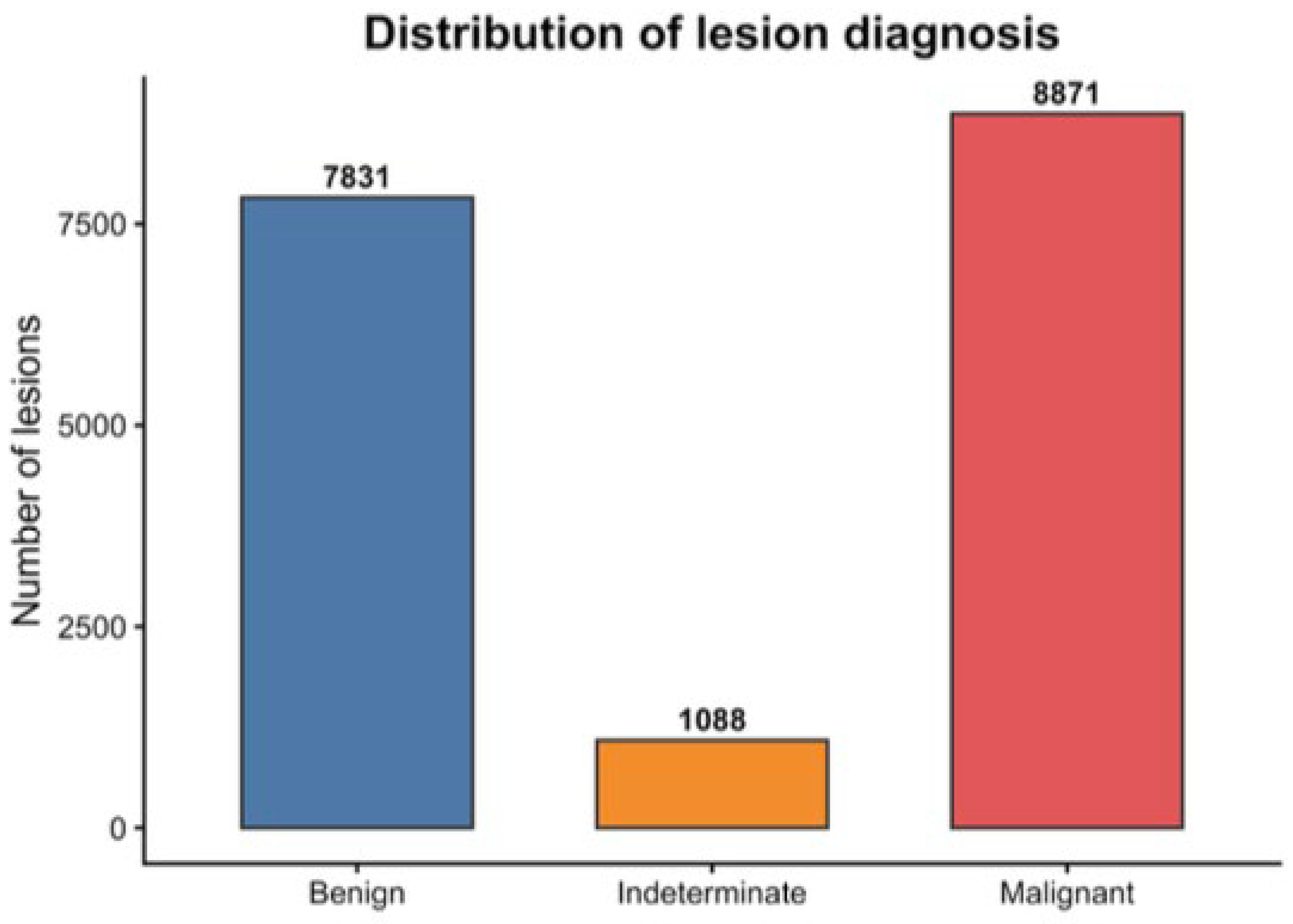
Figure 2.
Age distribution according to diagnostic category. The box-plots represent the median and interquartile range, while the red dots indicate the mean age within each diagnostic group.
Figure 2.
Age distribution according to diagnostic category. The box-plots represent the median and interquartile range, while the red dots indicate the mean age within each diagnostic group.
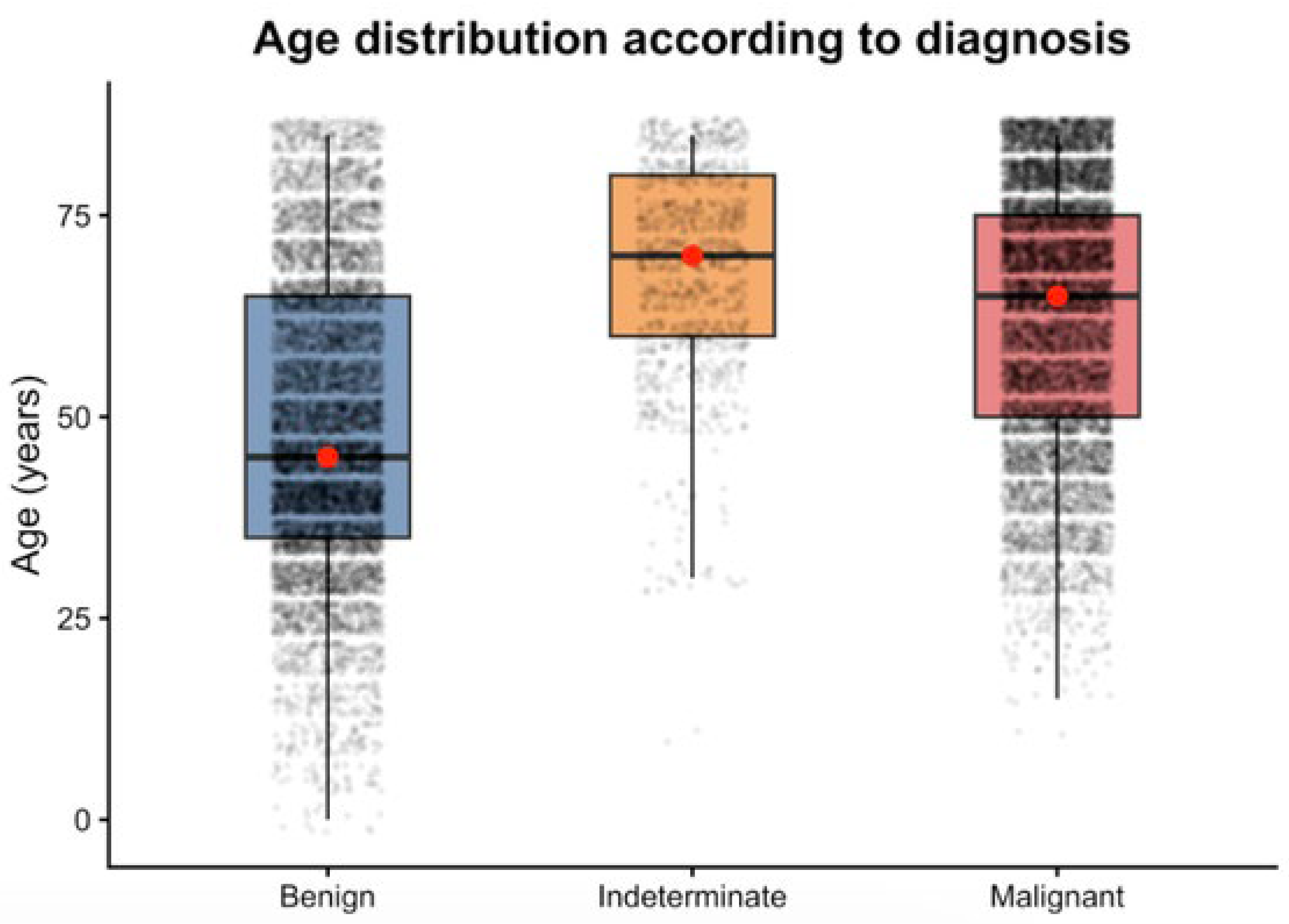
Figure 3.
Distribution of lesions according to anatomical site across the three diagnostic categories.
Figure 3.
Distribution of lesions according to anatomical site across the three diagnostic categories.
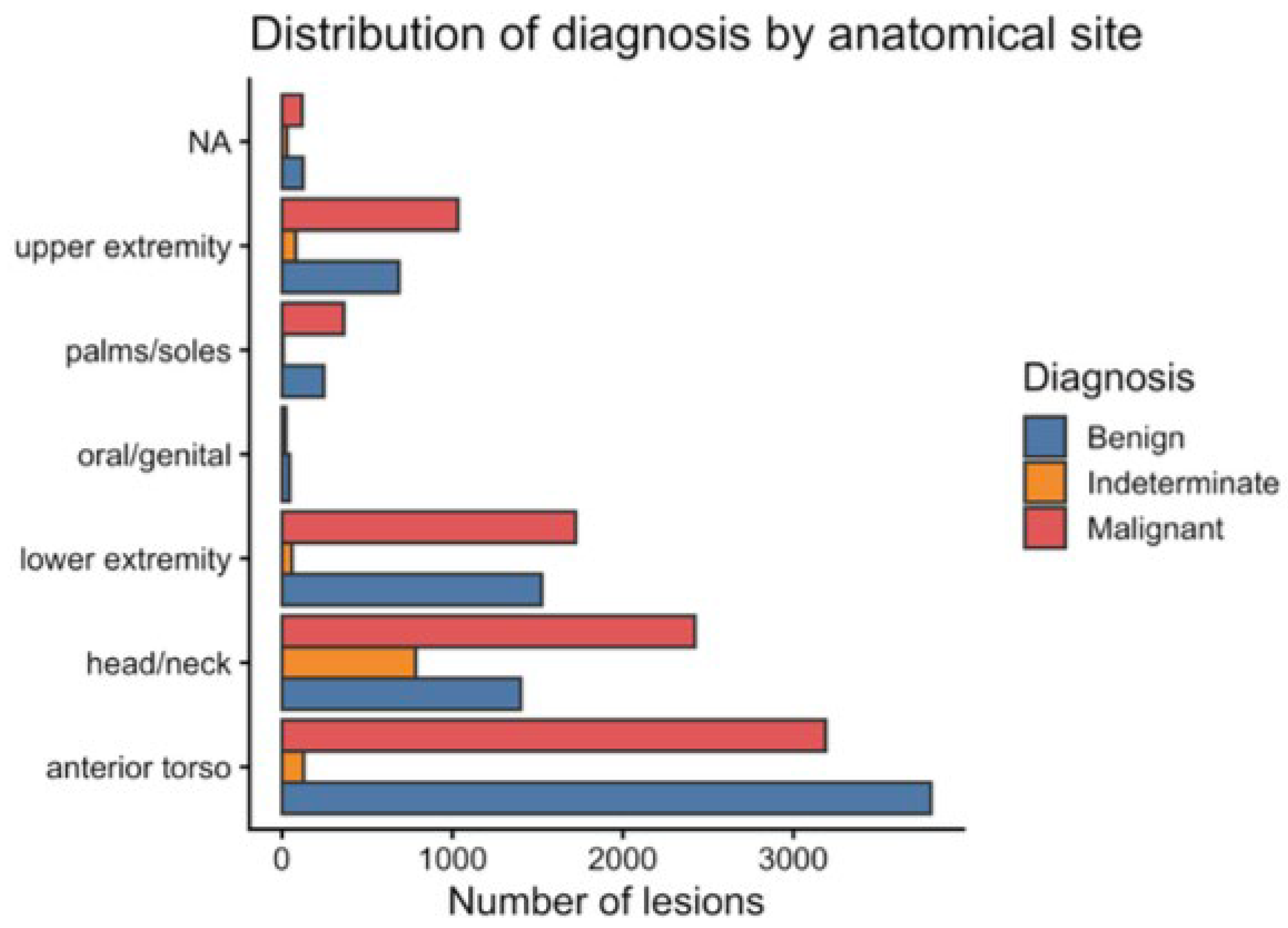
Figure 4.
Distribution of melanocytic status across the three diagnostic categories.
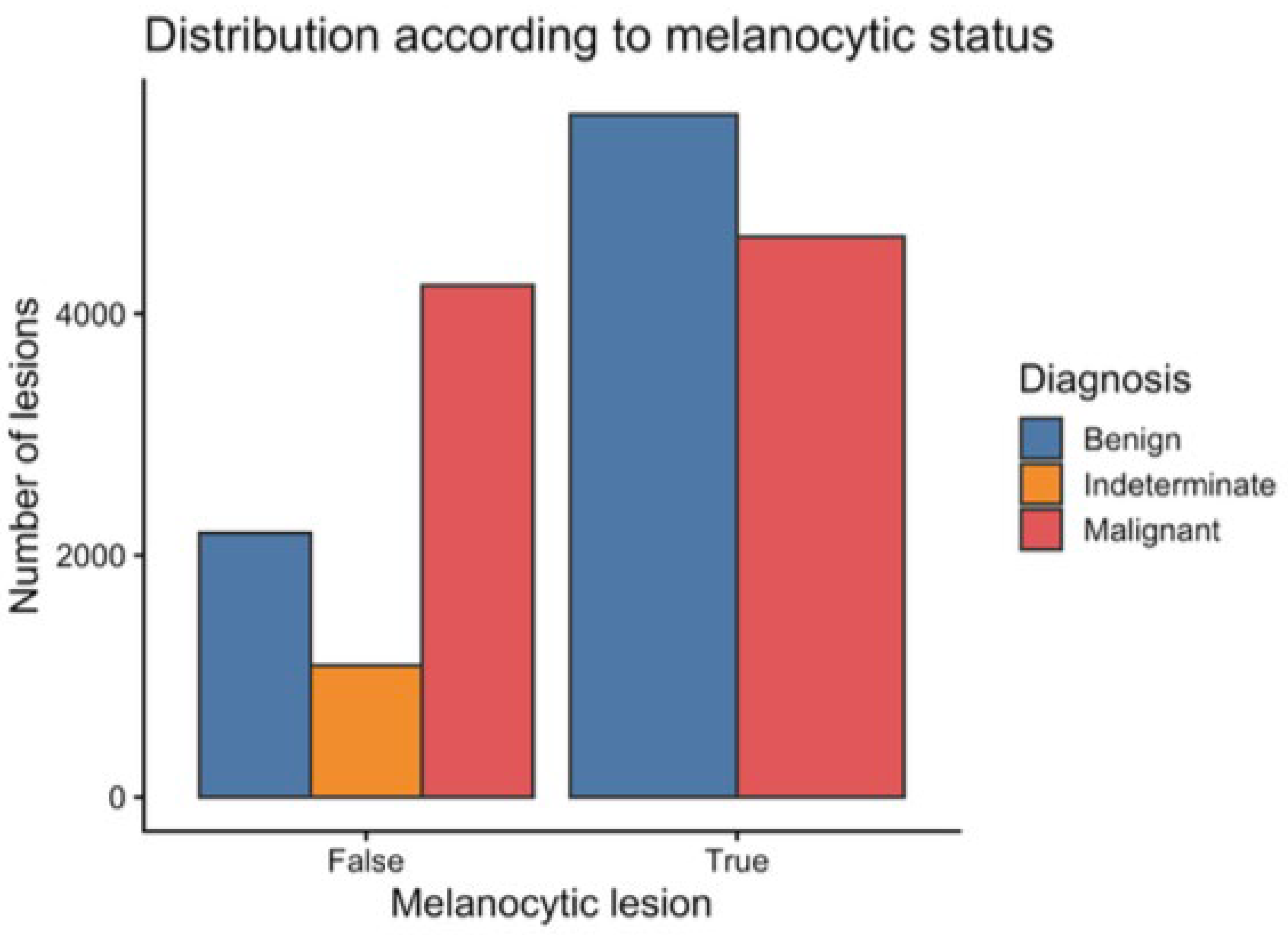
Figure 5.
Receiver Operating Characteristic (ROC) curves comparing the predictive performance of the four evaluated classification models on the independent testing set.
Figure 5.
Receiver Operating Characteristic (ROC) curves comparing the predictive performance of the four evaluated classification models on the independent testing set.
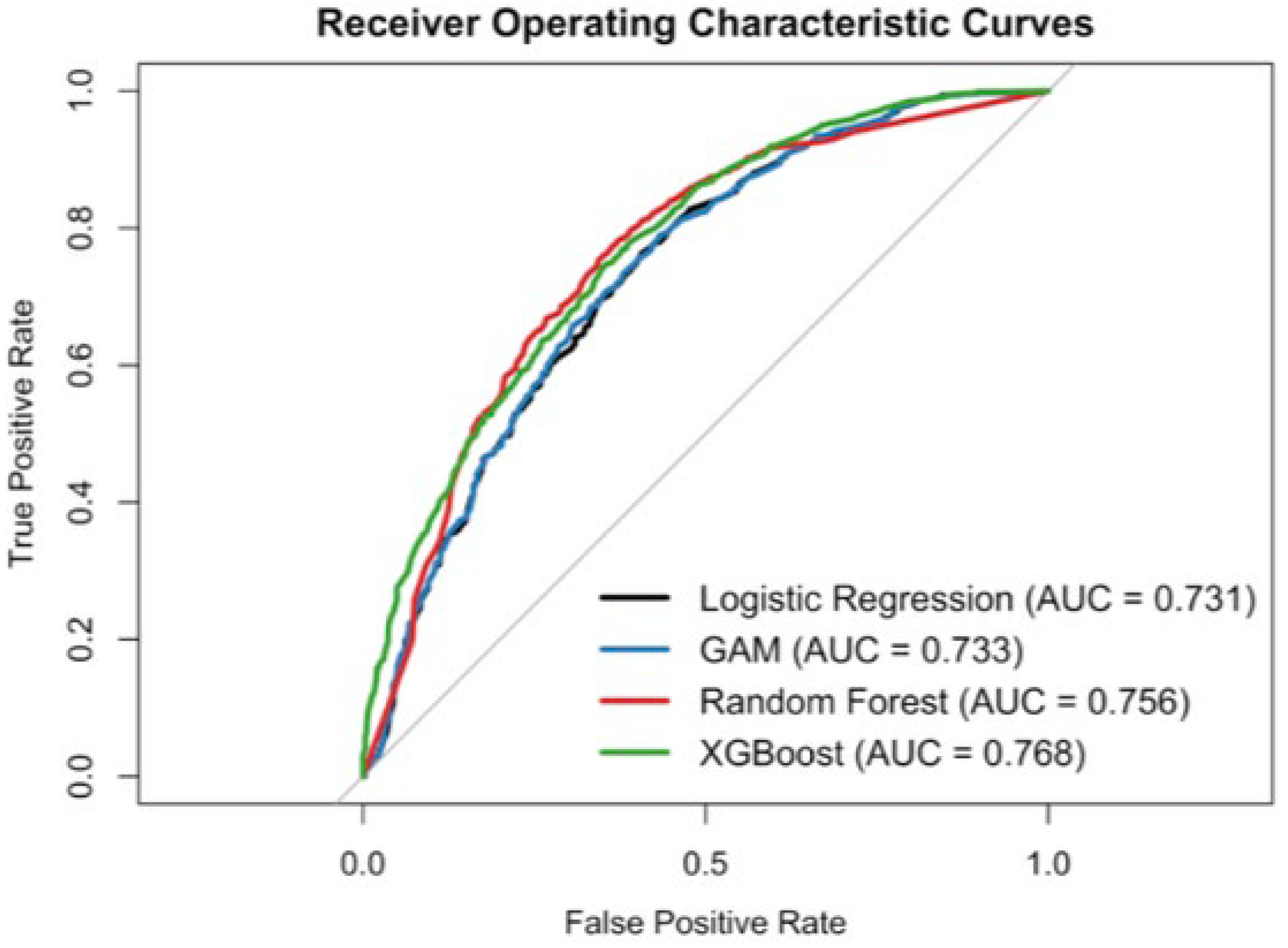
Figure 6.
Calibration plots of the evaluated classification models. The dashed diagonal line represents perfect calibration, whereas the solid lines illustrate the observed relationship between predicted and observed probabilities.
Figure 6.
Calibration plots of the evaluated classification models. The dashed diagonal line represents perfect calibration, whereas the solid lines illustrate the observed relationship between predicted and observed probabilities.
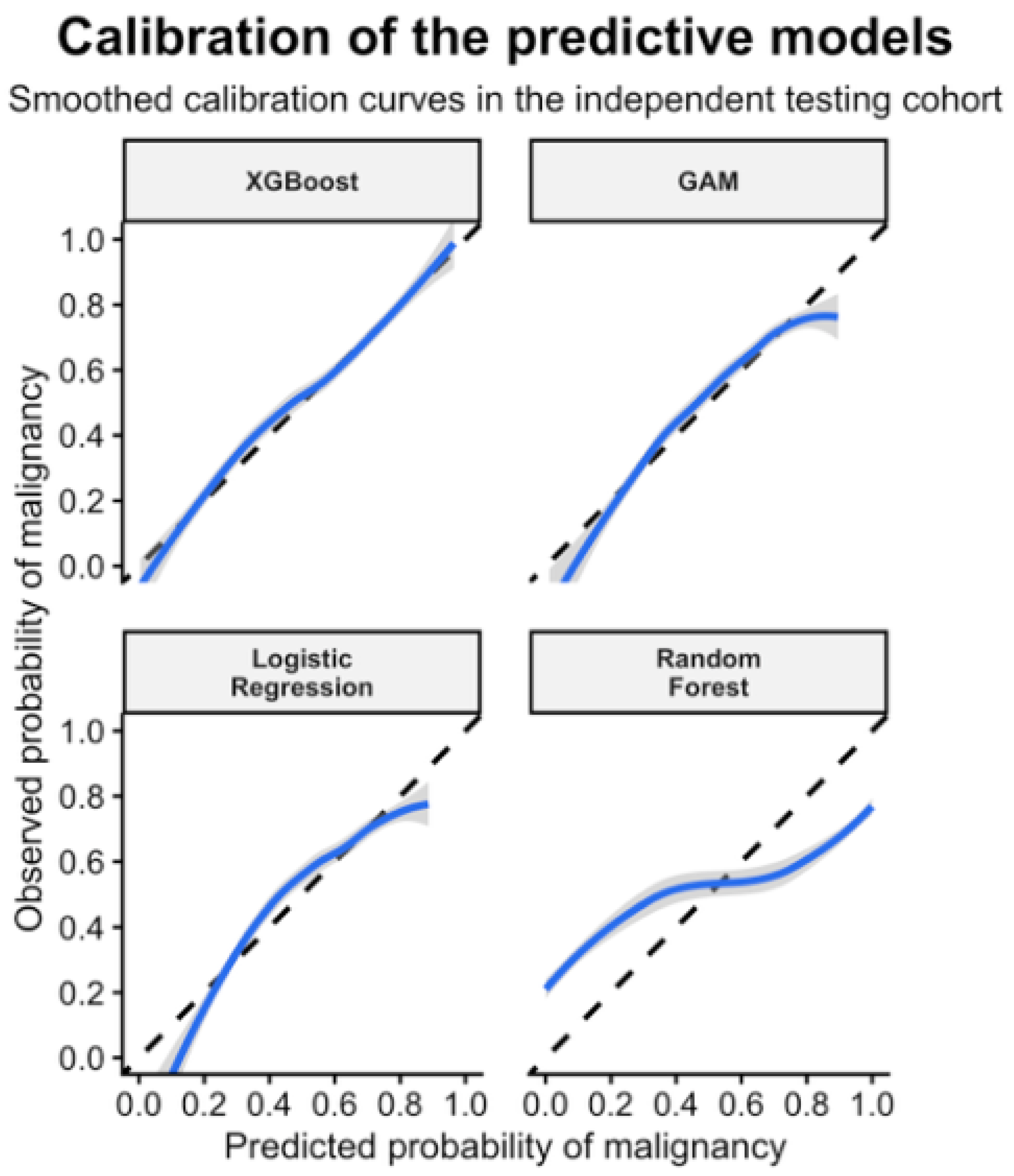
Figure 7.
SHAP summary (bees-warm) plot showing the global importance of the predictors included in the XGBoost model. Each point represents one lesion, with color indicating the feature value (low to high) and the horizontal position representing the corresponding SHAP value.
Figure 7.
SHAP summary (bees-warm) plot showing the global importance of the predictors included in the XGBoost model. Each point represents one lesion, with color indicating the feature value (low to high) and the horizontal position representing the corresponding SHAP value.
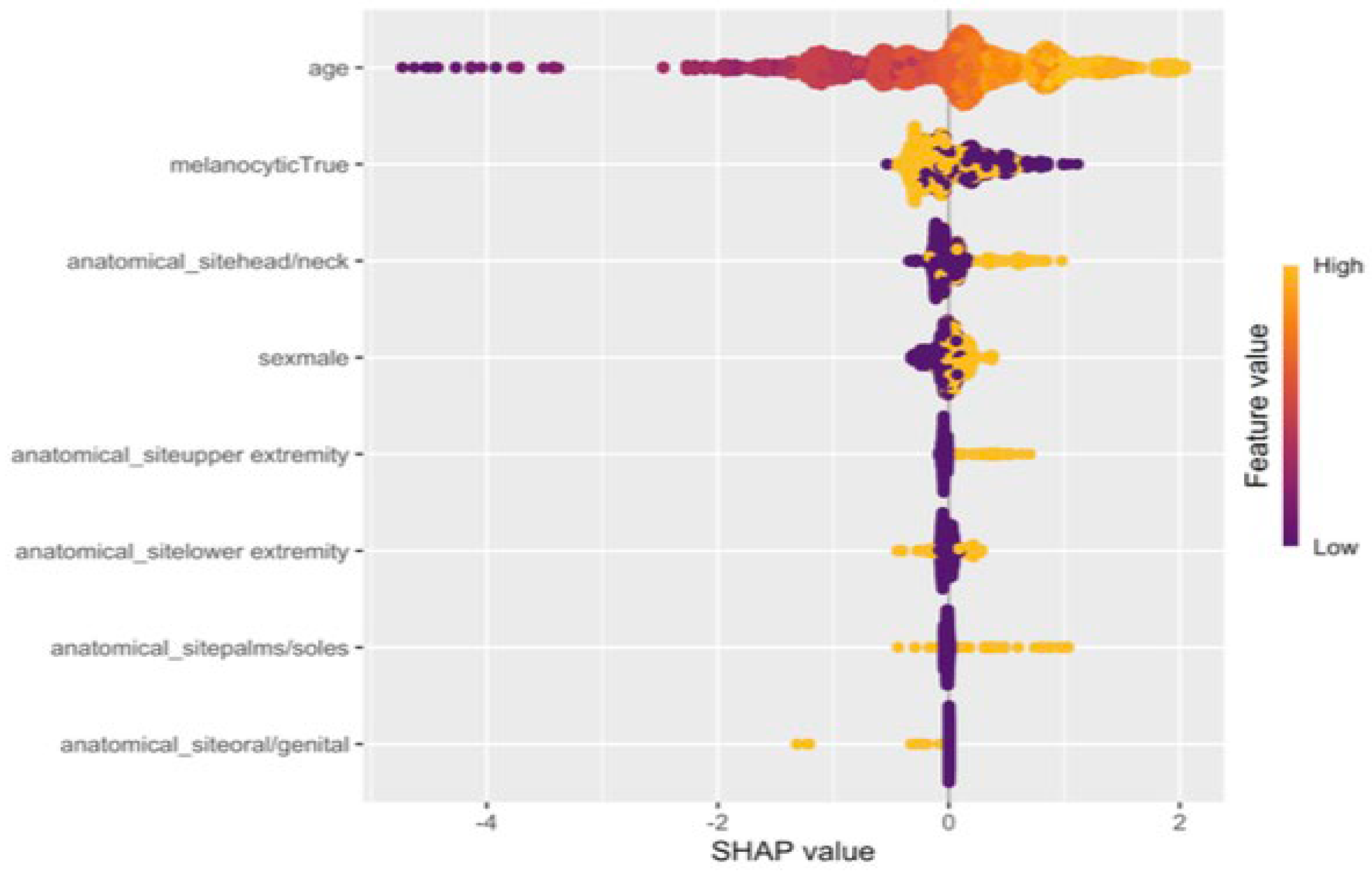
Figure 8.
SHAP dependence plot illustrating the relationship between age and its contribution to the XGBoost model predictions. Each point represents an individual lesion, with the SHAP value indicating the contribution of age to the predicted probability of malignancy.
Figure 8.
SHAP dependence plot illustrating the relationship between age and its contribution to the XGBoost model predictions. Each point represents an individual lesion, with the SHAP value indicating the contribution of age to the predicted probability of malignancy.
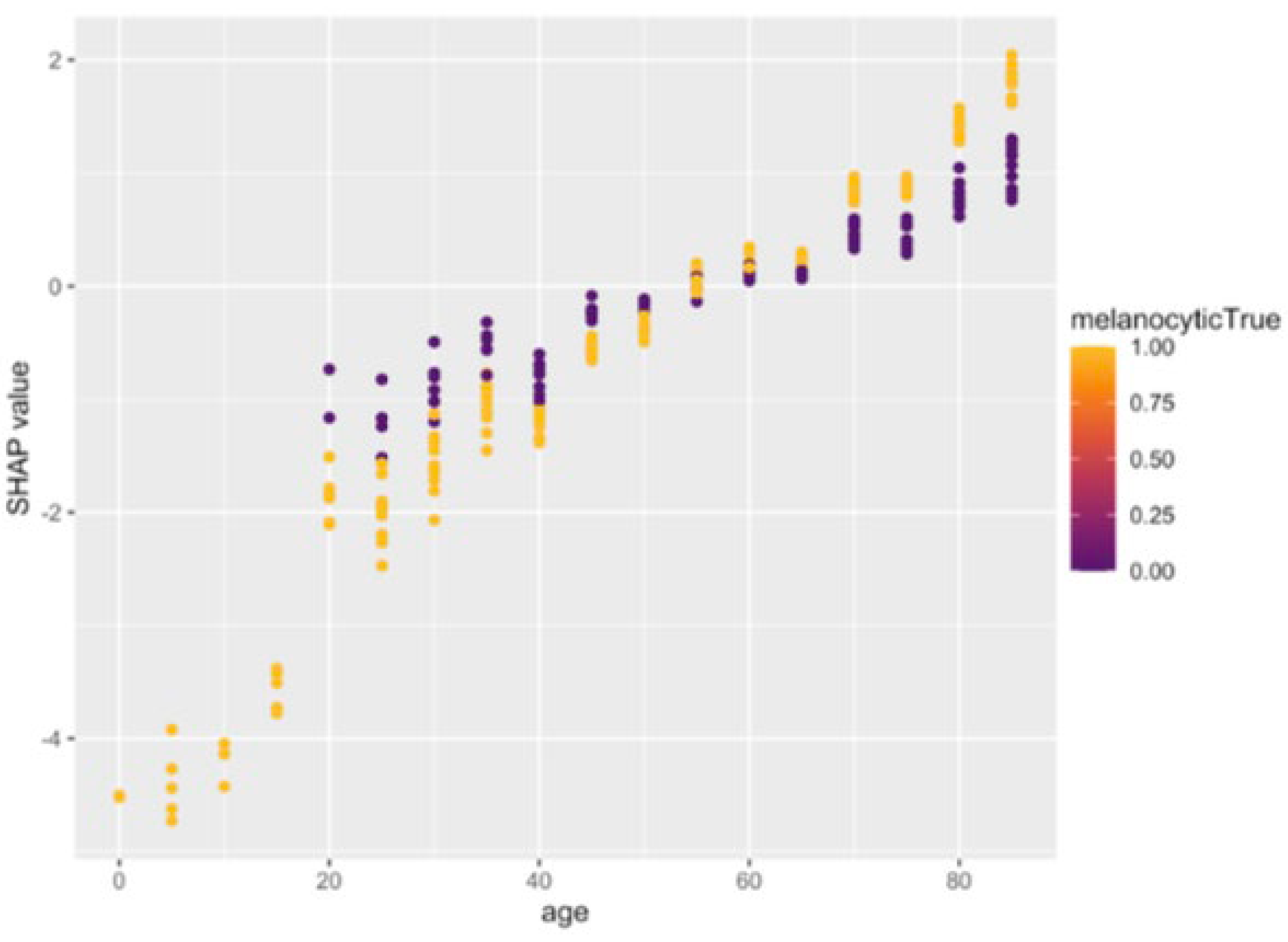

Table 1.
Baseline characteristics of lesions with a definitive diagnosis (N = 17,790). Lesions without a definitive diagnosis (n = 1,156) were excluded from diagnosis-specific descriptive analyses.
Table 1.
Baseline characteristics of lesions with a definitive diagnosis (N = 17,790). Lesions without a definitive diagnosis (n = 1,156) were excluded from diagnosis-specific descriptive analyses.
| Characteristics |
Overall N = 17790 |
Benign N = 7831 |
Indeterminate N = 1088 |
Malignant N = 8871 |
p-value |
| age | 60.0(45.0,75.0) | 45.0(35.0,65.0) | 70.0(60.0,80.0) | 65.0(50.0,75.0) | <0.001 |
| sex | <0.001 | ||||
| female | 8454(47.8%) | 4036(51.9%) | 519(47.8%) | 3899(44.2%) | |
| male | 9221(52.2%) | 3740(48.1%) | 566(52.2%) | 4915(55.8%) | |
| anatomical_site | <0.001 | ||||
| anterior torso | 7124(40.7%) | 3807(49.4%) | 128(12.1%) | 3189(36.4%) | |
| head/neck | 4608(26.3%) | 1401(18.2%) | 784(74.1%) | 2423(27.7%) | |
| lower extremity | 3305(18.9%) | 1523(19.8%) | 59(5.6%) | 1723(19.7%) | |
| oral/genital | 67(0.4%) | 44(0.6%) | 0(0%) | 23(0.3%) | |
| palms/soles | 615(3.5%) | 246(3.2%) | 6(0.6%) | 363(4.1%) | |
| upper extremity | 1799(10.3%) | 686(8.9%) | 81(7.7%) | 1032(11.8%) | |
| melanocityc | <0.001 | ||||
| true | 7507(42.2%) | 2184(27.9%) | 1088(100%) | 4235(47.7%) | |
| false | 10283(57.8%) | 5647(72.1%) | 0(0%) | 4636(52.3%) | |
Table 2.
Predictive performance of the evaluated classification models on the independent testing set. Performance is reported in terms of discrimination (AUC), classification accuracy, sensitivity, specificity, positive predictive value (PPV), negative predictive value (NPV), F1-score, balanced accuracy and Brier score.
Table 2.
Predictive performance of the evaluated classification models on the independent testing set. Performance is reported in terms of discrimination (AUC), classification accuracy, sensitivity, specificity, positive predictive value (PPV), negative predictive value (NPV), F1-score, balanced accuracy and Brier score.
| Model | AUC (95% CI) | Accuracy | Sensitivity | Specificity | PPV | NPV | F1 | Balanced Accuracy | Brier Score |
| 0.731(0.714—0.748) | 0.673 | 0.704 | 0.638 | 0.688 | 0.655 | 0.696 | 0.671 | 0.208 | |
| 0.733(0.716–0.750) | 0.678 | 0.726 | 0.623 | 0.686 | 0.667 | 0.705 | 0.675 | 0.207 | |
| 0.756(0.740–0.773) | 0.707 | 0.764 | 0.644 | 0.709 | 0.706 | 0.735 | 0.704 | 0.243 | |
| 0.768(0.752–0.783) | 0.698 | 0.771 | 0.616 | 0.695 | 0.703 | 0.731 | 0.693 | 0.194 |
Table 3.
Pairwise comparison of the areas under the receiver operating characteristic curves (AUCs) using DeLong’s test. P-values lower than 0.05 indicate statistically significant differences between the corresponding models.
Table 3.
Pairwise comparison of the areas under the receiver operating characteristic curves (AUCs) using DeLong’s test. P-values lower than 0.05 indicate statistically significant differences between the corresponding models.
| Model comparison | Z statistic | p-value | Adjusted p-value | Significant |
| LR vs GAM | -3.350 | <0.001 | 0.00162 | Yes |
| LR vs RF | -4.806 | <0.001 | <0.001 | Yes |
| LR vs XGBoost | -7.798 | <0.001 | <0.001 | Yes |
| GAM vs RF | -4.440 | <0.001 | <0.001 | Yes |
| GAM vs XGBoost | -7.425 | <0.001 | <0.001 | Yes |
| RF vs XGboost | -2.868 | 0.00412 | 0.00412 | Yes |
Disclaimer/Publisher’s Note: The statements, opinions and data contained in all publications are solely those of the individual author(s) and contributor(s) and not of MDPI and/or the editor(s). MDPI and/or the editor(s) disclaim responsibility for any injury to people or property resulting from any ideas, methods, instructions or products referred to in the content. |
© 2026 by the authors. Licensee MDPI, Basel, Switzerland. This article is an open access article distributed under the terms and conditions of the Creative Commons Attribution (CC BY) license (http://creativecommons.org/licenses/by/4.0/).
Copyright: This open access article is published under a Creative Commons CC BY 4.0 license, which permit the free download, distribution, and reuse, provided that the author and preprint are cited in any reuse.


