
Submitted:
28 July 2026
Posted:
31 July 2026
You are already at the latest version
Abstract
This paper aims to describe a synthesis procedure for discrete-time, energy-based regulators for continuous-time port-Hamiltonian systems. The methodology consists of three steps. The first deals with the definition of a discrete-time approximation of the plant, which is subsequently employed in the development of the control law. The discrete-time model is obtained from the continuous-time dynamics by replacing the gradient of the Hamiltonian function with a discrete gradient. In this way, passivity, with the energy as storage function, is preserved, although the resulting state equation is in implicit form. The second step concerns the control synthesis and extends the continuous-time energy-shaping plus damping injection design technique to the proposed class of discrete-time port-Hamiltonian systems. Finally, the last step addresses the interconnection between the digital controller and the continuous-time plant. The coupling is implemented via a zero-order hold and relies on the solution of an optimisation problem that determines the “best” and “minimal” correction to be applied to the nominal control action in order to achieve the same performance as that obtained when the regulator is connected in closed loop with the discrete-time model of the plant. This is the reference scenario used to develop and tune the control law. The complete procedure (time discretisation, control design, and coupling implementation) is illustrated through an example.
Keywords:
discrete-time systems
; port-Hamiltonian systems
; modeling
; control design
; passivity
1. Introduction
Port-Hamiltonian systems were introduced about thirty years ago to provide a unified framework for modeling lumped-parameter continuous-time physical systems, [1]. Over the past decades, several control synthesis methodologies have been developed, [2,3,4]. More recently, their discrete-time extension has become a popular framework for the geometric integration of ordinary differential equations (ODEs), paving the way for digital control system design. Time-integration schemes are designed to preserve either the “structure” or the “energy” of continuous-time systems, and the literature distinguishes between two main categories: symplectic and energy-preserving integrators. Discrete-time Hamiltonian and port-Hamiltonian systems based on symplectic integrators have been extensively employed, for example, in [5,6,7,8,9]. This work instead focuses on a class of port-Hamiltonian systems belonging to the family of energy-preserving integrators, [10,11], with a particular emphasis on discrete-time control design.
The discrete-time port-Hamiltonian systems considered in this paper constitute a simple extension of those proposed in [12,13,14,15,16,17,18] and are characterised by dynamics that depend on the discrete gradient of the Hamiltonian, ([10], Definition 3.1). Further details can be found in [19,20], while the extension to distributed-parameter systems is presented in [21,22]. This particular dynamic structure is useful for control synthesis because it directly yields an energy-balance relation for the discrete-time system, thereby simplifying both the design procedure and Lyapunov-based stability analysis. Its main drawback is that the state equation is implicit.
The control design procedure consists of three steps. The first is devoted to developing a discrete-time port-Hamiltonian approximation of the plant that belongs to the class illustrated before. Based on this discrete-time model, the second design step addresses the definition of the control action. One option is to rely on an extension of the energy-shaping plus damping-injection paradigm, [2], for which several contributions have already been presented in the literature, [9,12,19,20]. Here, we propose an extension of the Interconnection and Damping Assignment Passivity-based Control (IDA-PBC) framework, [3]. It is worth mentioning that notable contributions in this research area can also be found in [18,23,24]. The idea is to determine a state-feedback law capable of modifying the internal and dissipative structures of the open-loop system, as well as its Hamiltonian function. In particular, the “new” Hamiltonian is characterised by a (global) minimum at the desired configuration (energy shaping), while the dissipative structure is modified to introduce sufficient dissipation to make this minimum attractive (damping injection). As in continuous time, mapping the open-loop system into the desired closed-loop system requires solving a matching equation. In continuous time, this equation is a nonlinear partial differential equation (PDE), whereas in the digital case it is algebraic in the discrete gradient.
The feedback action acts on the system by modifying its energy function and “structure”. These are two effective degrees of freedom for shaping steady-state and transient behaviour. Since the design and tuning of the regulator are performed in discrete time, the remaining problem is to develop a strategy to couple the digital controller with the continuous-time plant. This constitutes the third and final step of the synthesis procedure. Within energy- or passivity-based frameworks, the problem of interfacing digital and physical systems is usually addressed by preserving the passivity of the interconnection, [25,26]. The idea, instead, is to design an interface that guarantees performance similar to that achieved when the (digital) controller is interconnected with the discrete-time approximation of the plant (i.e., in the reference design scenario), while introducing minimal variations in the nominal control action, [27]. One way to “measure” performance is to consider the variation of the closed-loop Hamiltonian (energy) function along system trajectories. If, at each sampling instant, it decreases at least as much as in discrete time, then no performance degradation occurs. These considerations lead to an optimization problem in which the cost function is the amplitude of the perturbation applied to the nominal control action, while the constraints are given by the continuous-time plant dynamics and an upper bound on the “desired” energy level at the end of the sampling interval. The design procedure is illustrated through the example of a two-degree-of-freedom planar manipulator.
The paper is organized as follows. In Section 2, a summary on discrete-time port-Hamiltonian systems is presented, while an overview of the energy-based control design and the IDA-PBC framework in discrete-time are discussed in Section 3. Section 4 contains the digital-to-analog interfaces arising from the solution of different optimization problems. The example is discussed in Section 5, where the complete design procedure is illustrated in detail. Conclusions are in Section 6.
2. Discrete-Time Port-Hamiltonian Systems
In this paper, we refer to the following class of continuous-time port-Hamiltonian systems, [1]:
In (1), and are the time and state variable, and , with , are the input and output, are such that and for all , is full-rank, is the Hamiltonian (energy) function, and the initial condition. The matrix-valued functions J and R represent the interconnection and the dissipative structures of the system, respectively. Along system’s trajectories we have that
so if H is lower-bounded, (1) is passive and H is the storage function.
The design of a digital control law for (1) relies on the discrete-time approximation proposed in [19,20]. In brief, such a discrete-time model is obtained at first by replacing the time derivative by the finite difference
being the time samples and , with and . Secondly, a discrete approximation of the gradient operator is adopted, see e.g. ([10], Definition 3.1).
Definition 1.
Let be a continuously differentiable function. A discrete gradient is a continuous map such that for all we have
Typical examples are the mean value discrete gradient [28] defined as
or the Gonzalez discrete gradient, [10]. For a quadratic function with , it is easy to check that .
If we combine (1), (3) and Definition 1, for any , the discrete-time formulation of the port-Hamiltonian dynamics for control design is, [19,20]:
with and initial condition . This class of discrete-time systems can be seen as an extension of [12,15,18]. The functions and are discrete approximations of J, R and G. More precisely, for all , we require that , , , , and . Admissible choices for are , or simply , and similarly for and . From (4) and (7), we get the discrete-time version of (2):
Example 1.
In the linear case, the port-Hamiltonian system (1) takes the following form:
where are constant and such that and , while is constant and full rank. In (9), the Hamiltonian function is quadratic, more precisely , with , which implies that . It is immediate to see that the discrete-time version of (9) is given by
Now, since the matrix is invertible because the eigenvalues of the matrix cannot have positive real part, the implicit state equation can be made explicit. Consequently, the state equation in (10) can be rewritten as
since , thus the explicit dynamics is described by a linear system with feedthrough.
Example 2.
Let us consider a mechanical system locally described by n configuration variables . The kinetic energy is , being for all q the generalized mass matrix, while we let to denote the potential energy. As illustrated in [1], if no constraints are present, the dynamics can be described by a port-Hamiltonian system in the form (1), more precisely:
where are the generalized momenta, the Hamiltonian function is the total energy
are the generalized forces and velocities, respectively. Besides, in (11), we assume that is full rank, while takes into account the viscous friction forces, if present. It is easy to see that the discrete-time approximation of (11) is
where B is a discrete approximation of B. For simplicity, we can set . Since the Hamiltonian function in (12) is non-quadratic, it is not always possible to employ the mean value discrete gradient, as obtaining an explicit expression for the integral in (6) may be difficult or even impossible. In such cases, one may either resort to an approximation of the integral or adopt a different discrete gradient, such as the Gonzalez discrete gradient, which is constructed by sampling the continuous one. Finally, note that the state equation in (13) is given in implicit form. Consequently, unlike the linear case discussed in Example 1, an explicit state-update equation cannot, in general, be derived.
Remark 1.
System (7) is not based on a particular discrete gradient, which turns out to be a degree-of-freedom at disposal to the designer, together with the expression of , and . Such a model for control design is a compromise between accuracy in the response and (numerical) complexity of the final control law. The drawback is that the state equation is implicit: this is the price to pay to have “for free” the energy-balance relation (8), which is the starting point for control design and stability analysis.
Remark 2.
As mentioned in Remark 1 and reported in Examples 1 and 2, the state equation in (7) is in implicit form. It can be made explicit, i.e. solved for in the linear case discussed in Example 1 because H is quadratic and J, R and G in (1) are constants. This approach has been followed in [12,18]. In the nonlinear case, however, it is necessary to keep such an implicit formulation. Based on passivity arguments and inspired by [29], under mild conditions on the structure of the system and on the discrete gradient, in [20] has been shown that trajectories exist independently from the sampling time. This is the same rationale pursued in [15] where a similar result has been proved under the hypothesis that the sampling time is sufficiently small. In this paper we assume that the dynamical equations are well-posed, so the next state can be always (at least numerically) computed.
3. Energy-Based Control Design in Discrete-Time
This section aims at generalising the Interconnection and Damping Assignment Passivity-Based Control (IDA-PBC) design methodology [3], originally developed for continuous-time port-Hamiltonian systems, to the discrete-time setting. Remarkable contributions in this direction include [18,23] and [24], the latter being specifically focused on mechanical systems. These methodologies aim at assigning an equilibrium to (7) by means of state feedback, while preserving the port-Hamiltonian structure. If the closed-loop system retains the port-Hamiltonian form, asymptotic convergence to can be established by relying on a balance relation similar to (8).
We start from the balance relation (8) for the open-loop dynamics (7), which can be compactly rewritten as
where takes into account the dissipated power during the k-th sampling interval. Similarly to the continuous-time case [2,3], the idea behind the design of an energy-based state-feedback controller is to find
so that the closed-loop dynamics obey the “new” balance relation
in which is a “desired” energy with a (local) minimum at , replaces the natural dissipation, increased to improve the convergence rate, and is the new passive output.
For simplicity, we assume that the matrix-valued functions J, R and G in (1) are constant, and consequently that their discrete-time counterparts , and in (7) are also constant. The general case, in which these matrices depend on the state, is more involved. Nevertheless, most of the results and considerations developed for the simplified setting can be extended to the state-dependent case. The most natural extension of the IDA-PBC approach to the discrete-time setting requires to determine the feedback law in (14) so that the state equation in (7) is mapped to
which represents the “target” or “desired” dynamics. In (16), we have that
are the desired Hamiltonian function, interconnection matrix and dissipative structure, respectively. It is immediate to see that, if we let
the target system (16) equipped with the output satisfies the balance relation (15).
The comparison between the open-loop dynamics (7) and the target one (16) shows that the control action modifies the energy and the interconnection and dissipative structures of the original system. As far as the so-called energy-shaping action is concerned, the function selected so that the closed-loop energy in (17) has a minimum in . Besides, is chosen to improve the convergence rate towards the minimum of the closed-loop energy function. A similar effect is achievable via output feedback (damping injection) by imposing that in (14), with the function such that for all , and defined in (18). The simplest damping injection law is
with and . Note that such a control action can be also applied to the open-loop system (7) by setting . If is the only invariant solution of the steady state, the “new” dissipative structure in the system forces the asymptotic stability of the equilibrium. With simple calculations, we get that , , and have to satisfy the matching equation:
In the next proposition, sufficient conditions for the solution of (20) so that the state-feedback action (14) asymptotically stabilises a (forced) equilibrium of (7) are presented. This result is an immediate extension of [20].
Proposition 1.
Denote by a (forced) equilibrium for (7), and let be a function such that
being G⊥ the full-rank left annihilator of G, i.e. . If
with , then there exists for which . Besides, if for all , we have that
then is the discrete gradient of , i.e. , and the control action (14) with
being G+ the pseudo-inverse of G, maps (7) to the discrete-time system (16) with Hamiltonian function, interconnection and dissipative structures defined in (17), and output (18). Finally, if
for all and for some , then is a locally stable equilibrium for the closed-loop system with . Furthermore, if the largest invariant set contained in
is , then is a locally asymptotically stable equilibrium for the closed-loop system with .
Proof.
The result can be proved in the same way as ([20], Proposition 3.1). Note that asymptotic stability is a consequence of the La Salle’s invariance principle. In fact, for the closed-loop system we have , thus the corresponding energy function decrease until the trajectories evolve inside the set (24). Since the largest invariant set contained in (24) equals , the result immediately follows. □
A crucial point in the methodology of Proposition 1 is the solvability of the matching equation (21), which can be re-written in terms of the discrete gradient of as
The simplest approach is to rely on the PDE that follows from (25) once , i.e.:
When the matrix-valued functions J, R, and G in (1) depend on the state variable x, it is not straightforward to derive a solution to (25) from its continuous-time counterpart (26). However, in the constant case considered in this paper, the function and the matrices and that satisfy (26) also satisfy (25). This result is summarized in the following corollary.
Corollary 1.
Proof.
Remark 3.
Since the control action (14) with defined in (22) and in (19) depends on , we have to investigate how to compute at step k. The first important assumption is that the closed-loop dynamics obtained from (7), (14) and (19) is well-posed, see ([20], Proposition 2.1). The corresponding state equation is
For (27) at each step k, we let
where . So, ξ is the solution of , with only in the nominal case, i.e. when the plant exactly behaves as (27), while (14) and (19) provide . This approach is conceptually similar to [9], where the control design problem is tackled for discrete-time models of mechanical systems in port-Hamiltonian form arising from symplectic integration schemes (i.e., the implicit midpoint rule). On the other hand, it differs from [12,18] where the implicit state equation is approximated with an explicit one.
Remark 4.
The key step in the procedure of Proposition 1 is to solve (21) for suitable matrices , , and , where must be the discrete gradient of a function . If the structure matrices of the port-Hamiltonian system (1) are not constant, Corollary 1 cannot be applied, and solving the matching equation may become considerably more involved. A different approach has been discussed in [20]. The idea is to exploit the algebraic nature of (21) to derive a broader class of control laws of the form (22), capable of performing an (approximate) energy-shaping action on the open-loop system (7) without requiring to be the discrete gradient of an energy function. This approach is the discrete-time extension of the technique proposed in [30]. This topic is beyond the scope of the present paper.
4. “Performance-Preserving” Coupling Strategies
The aim of this section is to present a strategy for coupling the discrete-time regulator designed according to the procedure illustrated in Section 3 with the continuous-time plant (1). Since the controller is designed on the basis of the discrete-time model (7), its performance is typically assessed through numerical simulations using the same model as a reference. The proposed coupling strategy therefore aims at applying the “smallest” perturbation to the nominal stabilising control law that guarantees performance as close as possible to that of the reference case. In particular, the transient and steady-state behaviours are preserved if the variation of the closed-loop Hamiltonian function defined in (17) along the system trajectories remains unchanged. These considerations lead to an optimization problem that must be solved at each step , resulting in a novel digital-to-analog interface.
For any energy-based control synthesis methodology such as the ones that fit into the framework illustrated in Section 3, let us consider a coupling algorithm based on the solution of the following nonlinear optimization problem at each step ,27]:
The idea is simple. At each , the state variable of (1) is acquired, and the control action (14) is computed by relying on the discrete-time model (7) in which . For simplicity and without loss of generality, in (14) we assume that , i.e. the required dissipation is introduced via the state feedback law . As discussed in Remark 3, the design procedure provides the “next” state and so, in the ideal case, the value of the closed-loop energy in is known and equal to . The digital-to-analog interface requires to compute the “smallest” perturbation to the nominal control input so that the control action applied to (1) during is admissible, i.e. it belongs to the set U, and the value of in is not greater than . The result is that the closed-loop energy function decreases at least as in the reference discrete-time case. The parameter is an upper bound for .
Remark 5.
The feasibility of (28) is not always guaranteed. This is the major issue of the approach since at every the perturbation has to be computed to obtain the control action . As in ([31] Theorem 2.5]), thanks to the Gronwall-Bellman inequality, it is possible to show that there could be sampling instants for which does not decrease as expected, i.e. that does not belong to the “desired” level set, as specified by the last inequality constraint in (28). A similar problem has been tackled in [25] by dissipating the difference between achieved and desired energy at in the next sampling interval(s). This strategy is applicable here, but this topic is not addressed in this paper. Soft constraints are a simple way to tackle the feasibility issue of (28) in a simple way. The corresponding optimization problem is
where we have removed the amplitude constraint on and assumed that . In (29), we let and , so the variable allows to dynamically relax the constraint on the closed-loop energy function at . The idea is to compute the “smallest” correction to the nominal control action so that the is as close as possible to the target value . The mismatch is reduced by selecting sufficiently large. It is easy to see that (29) is always feasible, and that existence of solution follows from the cost function being lower-bounded.
Noticeable limitations of (28) and (29) are that the constraint on depends on a nonlinear ODE and that the closed-loop Hamiltonian function is, in general, non-quadratic. Consequently, the real-time implementation of the coupling mechanism is potentially computationally demanding. Under a few conditions, an explicit solution is possible when the plant is linear and the closed-loop Hamiltonian is quadratic. The result is based on ([32], Proposition 1), reported below.
Proposition 2.
Let , and such that , and , with . The solution of the convex optimization problem
is
Let us consider the linear port-Hamiltonian system (9), which can be rewritten in the form with , , and . Let us also assume that the discrete-time control design procedure assigns target dynamics in port-Hamiltonian form with quadratic Hamiltonian
With simple computations, it is easy to see that, at the end of the k-th sampling interval, starting from and under the control input , (9) reaches
where
Consequently, the energy constraint in (28) takes the form of the quadratic constraint in (30), with , , and . Thus, the coupling strategy is recast as the optimization problem of Proposition 2, in which . Consequently,
where . Note that this result can be used to address the general nonlinear case approximately, by relying, at each sampling interval , on a linear approximation of the plant dynamics around .
5. Numerical Example: The 2-Dof Planar Robotic Manipulator
Let us consider the two degrees-of-freedom planar manipulator of Figure 1, which belongs to the class illustrated in Example 2.
The generalised coordinates are , and the total energy is (12) in which the inertia matrix is
and the potential energy is
with g the gravity acceleration. The continuous-time model is (11), with and , where . The inputs are the torques at each joint. The parameters are reported in Table 1.
The discrete-time approximation of the plant model is (13), and in the numerical examples, the mean value discrete gradient (6) is employed. Note that from (34), for any , we have that
where and
Based on the general framework summarized in Proposition 1, it is easy to check that the matching equation (21) with is satisfied if depends on the displacements only. As a consequence, the control action only shapes the potential energy. The simplest choice is to have , with , so that the desired Hamiltonian function has a global minimum in , which means that the conditions (23) are satisfied.. It is interesting to note that an explicit expression for can be computed based on (35) and on the fact that the further term in is quadratic. This leads to the PD plus gravity compensation controller. Asymptotic convergence to the global minimum of is obtained via the damping injection law (19), where is the output of either the plant and of the closed-loop system. As far as the controller parameters are concerned, we have that and .
The block diagram of the complete system resulting from the coupling of the discrete-time controller and the continuous-time plant is reported in Figure 2 to show how the control action is implemented in practice.
Since the stabilising law is based on state-feedback, the starting point is to sample the state of the plant in . The sampled variable is used to determine the “desired” next state according to the target dynamics. As discussed in Remark 3, the discrete variable has been introduced to distinguish from that denotes the sampled value of in . Getting requires the solution of an implicit equation. This step is represented by the grey box. Based on and , the control action is computed, while the “corrective” term follows from the strategies discussed in Section 4. In both the cases, we let .
At first, the behaviour obtained in the discrete-time case, i.e. when the control law is applied to the discrete-time formulation (13) of the plant, is reported in Figure 3.
As a matter of fact, this represent the desired response that the designer aims at achieving when the digital controller is coupled with the “real” plant or, in this case, to its continuous-time model (11). The synthesis of the control law and the tuning of the regulator parameters is carried out in the discrete-time setting, and the idea is to get analogous performances in the real-world scenario. Starting from the top graph of Figure 3, the evolution of the discrete displacements , of the control input and of the closed-loop Hamiltonian function are reported. This latter response summarizes the transient behaviour of the controlled system and it is the main information required by the coupling techniques discussed in Section 4.
We analyse the coupling strategy based on the optimization problem (29) in which . This sub-optimal formulation of (28) has been preferred because it does not suffer from any feasibility issue. It is worth mentioning, however, that for the specific case discussed here (28) is always feasible. The closed-loop system behaviour is reported in Figure 4 and Figure 5. A comparison between Figure 3 and Figure 4 shows that the performances obtained when the discrete-time controller is coupled with the continuous-time plant are practically the same as in the reference case. The role of the interconnection mechanism is summarized in Figure 5. The correction term is different from 0 only in the initial part of the transitory and its amplitude is noticeably lower than the nominal control action . The design procedure carried out in discrete-time by relying on the class of implicit port-Hamiltonian systems (7) or (13), in this specific case, ensures very good performances by its own. Consequently, the constraint on the amplitude of , i.e. the parameter that appears in the optimization problem (28), is not strictly necessary from a “practical” point of view in a real-world scenario. In some sense, this motivates the choice carried out to define the optimization problem (29) with the goal of not having any feasibility issues.
In the graph at the bottom of Figure 5, the evolution of is reported. Such a quantity represents the difference between target and achieved closed-loop Hamiltonian at each sample instant. In other words, at each sampling interval k, the variable is computed. It represents the next state according to the desired evolution of the controlled system in discrete-time. This means that is the target value for the closed-loop energy to be reached at the end of the sampling interval, i.e. in . The coupling strategy should assure that is lower or equal than . Note that in Figure 5 is coherent with such a desired behaviour, which means that the reference performances of the discrete-time scenario are obtained in the mixed discrete-continous-time case.
6. Conclusions and Future Activities
This paper presented a complete synthesis procedure for the design and implementation of energy-based digital controllers for port-Hamiltonian systems. The procedure consists of three main steps. First, a discrete-time port-Hamiltonian approximation of the plant is obtained by “replacing” the Hamiltonian gradient with a discrete gradient. This construction preserves the energy-balance relation of the continuous-time system, although it generally leads to implicit state equations. Second, an extension of the IDA-PBC methodology to the resulting class of discrete-time systems is presented. The proposed design reshapes the Hamiltonian function and modifies the interconnection and dissipative structures in order to assign a desired equilibrium and guarantee its asymptotic stability under suitable conditions. The third step addresses the interconnection between the digital controller and the continuous-time plant. A performance-preserving digital-to-analog interface is proposed, based on the solution of an optimization problem that computes the smallest correction to the nominal control action required to enforce a desired decrease of the closed-loop Hamiltonian over each sampling interval. A soft-constrained formulation is also considered to address possible feasibility issues. For linear systems with quadratic desired Hamiltonians, the optimization problem admits an explicit solution. The complete procedure was illustrated using a two-degree-of-freedom planar manipulator. The numerical results show that the proposed interface allows the mixed discrete-continuous-time closed-loop system to reproduce closely the response obtained in the reference discrete-time design scenario, while requiring only a small correction to the nominal control action, mainly during the initial transient.
Future work will focus on extending the proposed discrete-time IDA-PBC framework to systems with state-dependent structure matrices, for which solving the matching equation is more challenging. Further research will also address computationally efficient implementations of the coupling strategy for nonlinear systems, the treatment of feasibility issues over successive sampling intervals, and experimental validation on physical systems.
References
- van der Schaft, A. L2-Gain and Passivity Techniques in Nonlinear Control. In Communication and Control Engineering, 3rd ed.; Springer International Publishing AG: Cham, Switzerland, 2017. [Google Scholar]
- Ortega, R.; van der Schaft, A.; Mareels, I.; Maschke, B. Putting energy back in control. In Control Systems Magazine; IEEE, 2001; pp. 18–33. [Google Scholar]
- Ortega, R.; van der Schaft, A.; Maschke, B.; Escobar, G. Interconnection and damping assignment passivity-based control of port-controlled Hamiltonian systems. Automatica 2002, 38, 585–596. [Google Scholar] [CrossRef]
- Fujimoto, K.; Sugie, T. Canonical transformation and stabilization of generalized Hamiltonian systems. Syst. Control Lett. 2001, 42, 217–227. [Google Scholar] [CrossRef]
- Ruth, R. A Canonical Integration Technique. Nucl. Sci. IEEE Trans. 1983, 30, 2669–2671. [Google Scholar]
- Gonzalez, O.; Simo, J. On the stability of symplectic and energy-momentum algorithms for non-linear Hamiltonian systems with symmetry. Comput. Methods Appl. Mech. Eng. 1996, 134, 197–222. [Google Scholar] [CrossRef]
- Marsden, J.; West, M. Discrete mechanics and variational integrators. Acta Numer. 2001, 10, 357–514. [Google Scholar] [CrossRef]
- Kotyczka, P.; Lefèvre, L. Discrete-time port-Hamiltonian systems: A definition based on symplectic integration. Syst. Control Lett. 2019, 113, 104530. [Google Scholar] [CrossRef]
- Kotyczka, P.; Thoma, T. Symplectic discrete-time energy-based control for nonlinear mechanical systems. Automatica 2021, 133, 109842. [Google Scholar] [CrossRef]
- Gonzalez, O. Time integration and discrete Hamiltonian systems. J. Nonlinear Sci. 1996, 6, 449–467. [Google Scholar] [CrossRef]
- Quispel, G.; Turner, G. Discrete gradient methods for solving ODEs numerically while preserving a first integral. J. Phys. A Math. General. 1996, 29, L341. [Google Scholar] [CrossRef]
- Gören-Sümer, L.; Yalçin, Y. Gradient Based Discrete-Time Modeling and Control of Hamiltonian Systems. In Proceedings of the 17th IFAC World Congress, Seoul, Korea, July 6-11 2008; pp. 212–217. [Google Scholar]
- Monaco, S.; Normand-Cyrot, D.; Tiefensee, F. Nonlinear port controlled Hamiltonian systems under sampling. In Proceedings of the 49th IEEE Conference on Decision and Control (CDC 2010), Atlanta, Georgia, USA, Dec. 15-17 2010; pp. 1782–1787. [Google Scholar]
- Celledoni, E.; Høiseth, E. Energy-Preserving and Passivity-Consistent Numerical Discretization of Port-Hamiltonian Systems. arXiv 2017, arXiv:1706.08621. [Google Scholar]
- Aoues, S.; Di Loreto, M.; Eberard, D.; Marquis-Favre, W. Hamiltonian systems discrete-time approximation: Losslessness, passivity and composability. Syst. Control Lett. 2017, 110, 9–14. [Google Scholar] [CrossRef]
- Moreschini, A.; Mattioni, M.; Monaco, S.; Normand-Cyrot, D. Discrete port-controlled Hamiltonian dynamics and average passivation. In Proceedings of the IEEE 58th Annual Conference on Decision and Control (CDC), Nice, France, Dec. 11-13 2019; pp. 1430–1435. [Google Scholar]
- Moreschini, A.; Monaco, S.; Normand-Cyrot, D. Gradient and Hamiltonian dynamics under sampling. In Proceedings of the 11th IFAC Symposium on Nonlinear Control Systems, NOLCOS 2019; Jadachowski, L., Ed.; Vienna, 4-6 Sep 2019. [Google Scholar]
- Moreschini, A.; Mattioni, M.; Monaco, S.; Normand-Cyrot, D. Stabilization of discrete port-Hamiltonian dynamics via interconnection and damping assignment. IEEE Control Syst. Lett. 2021, 5, 103–108. [Google Scholar] [CrossRef]
- Macchelli, A. Trajectory Tracking for Discrete-Time Port-Hamiltonian Systems. IEEE Control Syst. Lett. 2022, 6, 3146–3151. [Google Scholar] [CrossRef]
- Macchelli, A. Control Design for a Class of Discrete-Time Port-Hamiltonian Systems. Autom. Control IEEE Trans. 2023, 68, 8224–8231. [Google Scholar] [CrossRef]
- Macchelli, A. A Discrete-Time Formulation of Nonlinear Distributed-Parameter Port-Hamiltonian Systems. IEEE Control Syst. Lett. 2024, 8, 802–807. [Google Scholar] [CrossRef]
- Macchelli, A. Port-Hamiltonian Boundary Control Systems in Discrete-Time. Modelling and Control Design. Autom. Control IEEE Trans. 2026, 71, 722–736. [Google Scholar] [CrossRef]
- Gören-Sümer, L.; Yalçin, Y. A Direct Discrete-time IDA-PBC Design Method for a Class of Underactuated Hamiltonian Systems. In Proceedings of the 18th IFAC World Congress, Milan, Aug.-1 Sep. 2011. [Google Scholar]
- Aoues, S.; Eberard, D.; Marquis-Favre, W. Discrete IDA-PBC control law for Newtonian mechanical port-Hamiltonian systems. In Proceedings of the IEEE 54th Annual Conference on Decision and Control (CDC), Osaka, Japan, Dec. 15-18 2015; pp. 4388–4393. [Google Scholar]
- Stramigioli, S.; Secchi, C.; van der Schaft, A.; Fantuzzi, C. Sampled Data Systems Passivity and Discrete Port-Hamiltonian Systems. Robot. IEEE Trans. 2005, 21, 574–587. [Google Scholar] [CrossRef]
- Costa-Castelló, R.; Fossas, E. On Preserving Passivity in Sampled-data Linear Systems. Eur. J. Control 2007, 13, 583–590. [Google Scholar] [CrossRef]
- Macchelli, A. On the Synthesis of Discrete-time Energy-based Regulators for Port-Hamiltonian Systems. In Proceedings of the 22nd IFAC World Congress, Yokohama, Japan, July 9-14 2023; pp. 2889–2894. [Google Scholar]
- Harten, A.; Lax, P.; Van Leer, B. On Upstream Differencing and Godunov-Type Schemes for Hyperbolic Conservation Laws. SIAM Rev. 1983, 25, 35–61. [Google Scholar] [CrossRef]
- Ehrhardt, M.; Riis, E.; Ringholm, T.; Schönlieb, C.B. A geometric integration approach to smooth optimisation: Foundations of the discrete gradient method. arXiv 2020, arXiv:1805.06444. [Google Scholar]
- Nunna, K.; Sassano, M.; Astolfi, A. Constructive Interconnection and Assignment for Port-Controlled Hamiltonian Systems. Autom. Control IEEE Trans. 2015, 60, 2350–2361. [Google Scholar] [CrossRef]
- Khalil, H. Nonlinear Systems, 2nd ed.; Prentice Hall, 1996. [Google Scholar]
- Krupa, P.; Jaouani, R.; Limon, D.; Alamo, T. A Sparse ADMM-Based Solver for Linear MPC Subject to Terminal Quadratic Constraint. Control Syst. Technol. IEEE Trans. 2024, 32, 2376–2384. [Google Scholar] [CrossRef]
Figure 1.
The two degrees-of-freedom planar manipulator.
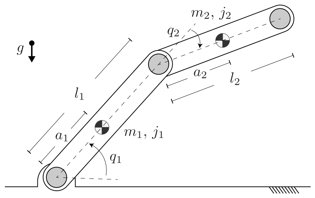
Figure 2.
Schematic representation of the closed-loop system.
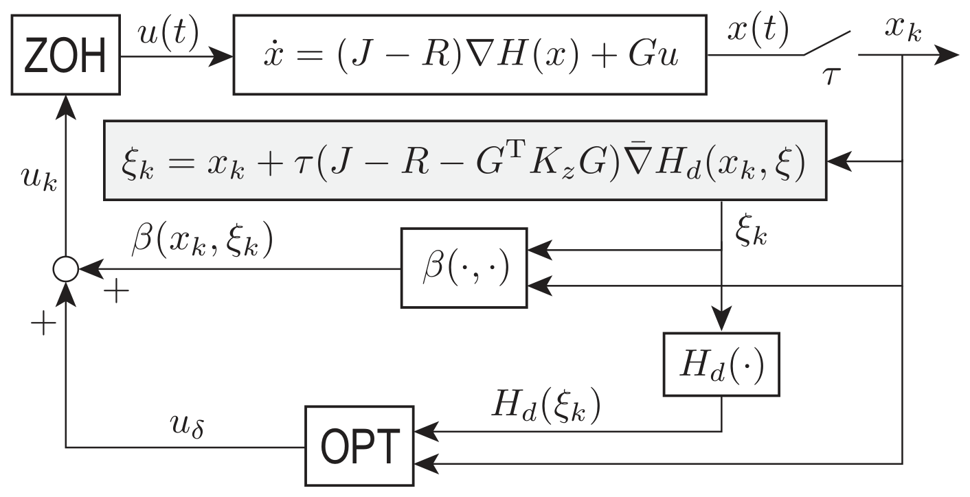
Figure 3.
Response in discrete-time (reference scenario).
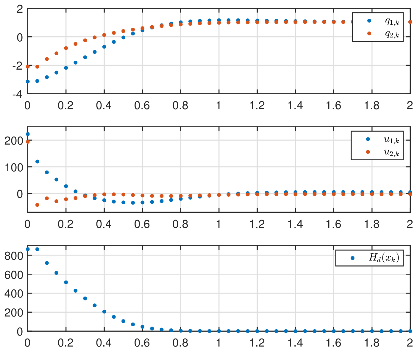
Figure 4.
Response with obtained thanks to (29).
Figure 4.
Response with obtained thanks to (29).
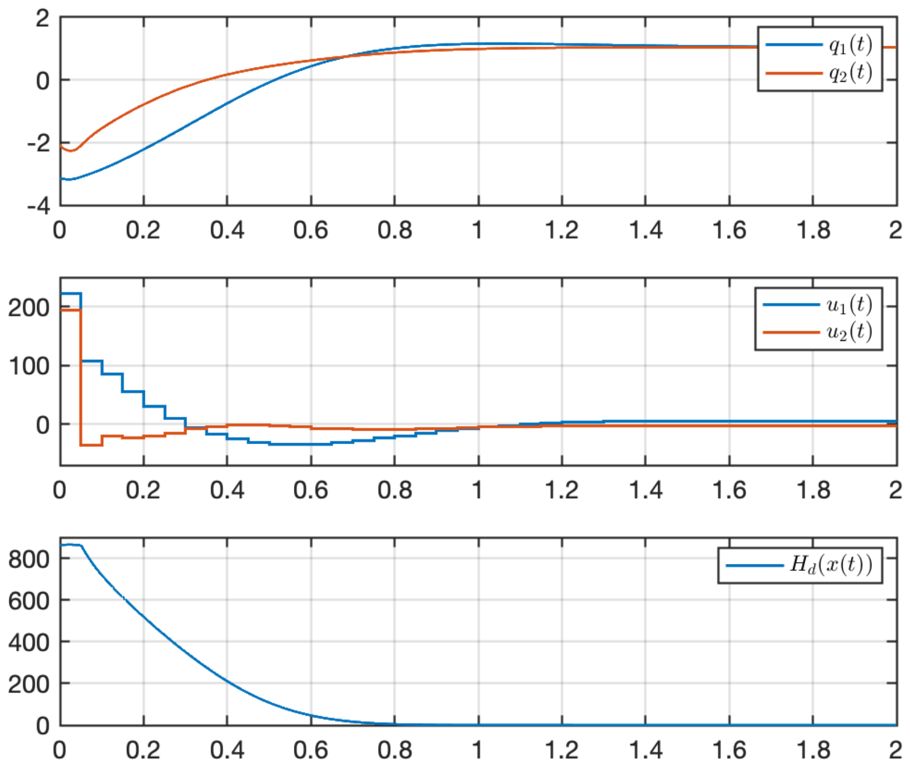
Figure 5.
Behaviour of the coupling strategy based on (29).
Figure 5.
Behaviour of the coupling strategy based on (29).
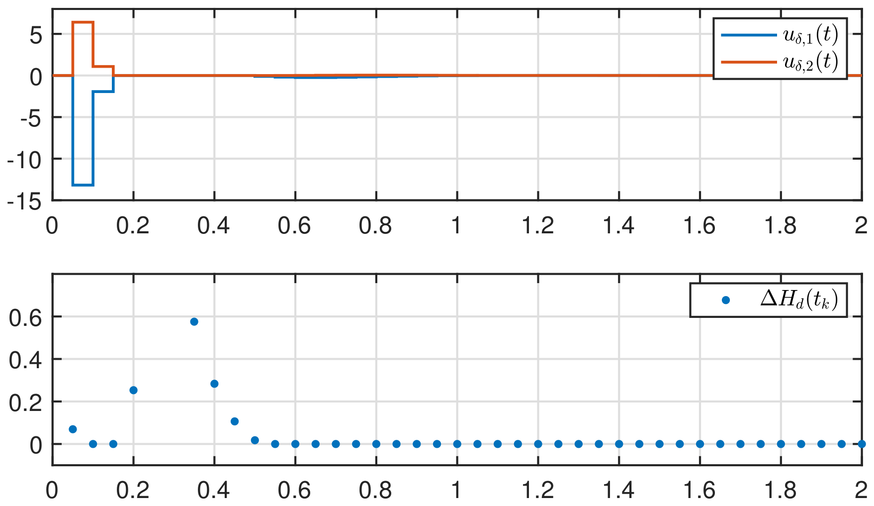

Table 1.
Parameters of the robot in Figure 1.
Table 1.
Parameters of the robot in Figure 1.
| parameter | value | parameter | value |
|---|---|---|---|
| 1 | |||
| 1 | |||
| d | |||
Disclaimer/Publisher’s Note: The statements, opinions and data contained in all publications are solely those of the individual author(s) and contributor(s) and not of MDPI and/or the editor(s). MDPI and/or the editor(s) disclaim responsibility for any injury to people or property resulting from any ideas, methods, instructions or products referred to in the content. |
© 2026 by the authors. Licensee MDPI, Basel, Switzerland. This article is an open access article distributed under the terms and conditions of the Creative Commons Attribution (CC BY) license (http://creativecommons.org/licenses/by/4.0/).
Copyright: This open access article is published under a Creative Commons CC BY 4.0 license, which permit the free download, distribution, and reuse, provided that the author and preprint are cited in any reuse.


