

Submitted:
29 July 2026
Posted:
30 July 2026
You are already at the latest version
Abstract
This paper aims to enhance Smith-predictor-based control systems (SPCSs) for multi-input multi-output (MIMO) time delay processes. Conventional SPCSs for MIMO processes are composed of an array of classical feedback controller(s). These controllers act on error signals, calculated through deducting a predicted output by a Smith predictor from a reference signal at the time of operation. Investigations on underperformance of conventional SPCSs identified two major shortcomings: (i) the design of classical feedback controllers is based on trade-off, and their use may lead to windup phenomenon, this adversely influences conventional SPCSs performance, (ii) a predicted output by a Smith predictor belongs to a time in the future and does not concurrent with the reference at the time of operation; that is, in conventional SPCSs, the control error is generated using two asynchronous signals. This paper proposes an enhanced SPCS design method for MIMO time-delay systems based on two enhancements to tackle the aforementioned dual shortcomings. The proposed control system evidently outperforms a conventional SPCS with proportional-integral-derivative (PID) feedback controllers. The case study is a catalytic stirred tank reactor (CSTR) with three inputs (feed and water flow rates and auxiliary temperature), two outputs (output flow concentration and temperature) and three time delays. The presented model of the CSTR is more comprehensive than any CSTR model found in the literature.
Keywords:
Smith predictor
; time delay system
; CSTR
; MIMO
; feedforward
; asynchrony
1. Introdction
Many dynamic systems witness dead-time or delay and are categorised as time-delay systems [1,2,3,4,5]. These include chemical processes, engines, manufacturing and telecommunication systems, etc. [6,7,8,9,10,11,12,13] . Time-delay is largely regarded as a source of instability and poor performance in control systems [14,15]. There are two categories of time-delay systems, widely known as network-induced and input-delay [16]. Network-induced delay is caused by the time needed to exchange data between devices in electrical/communication networks. In this category, states of a system affect their time derivatives with a delay. Control of system with network-induced time-delay is addressed using Lyapunov-Krasovskii and Razumikhin theorems [17,18] and is out of the scope of process control and this paper. On the other hand, in input-delay category, the control inputs affect the time derivatives of the system states with a delay, i.e. the actuator(s) affect the system after a non-negligible time [19,20]. This category of time-delay is a serious concern in process control [21,22] and is the focus of this paper.
Two main approaches have been employed to design model-based control systems for processes with input-delay: (i) integrating the delay into the model prior to control system design and (ii) the use of predictors/predictive models. Recently, the first approach has been used to design discrete/digital control but only for electromechanical systems with very short (<10 ms) delays [23,24] and not yet for process control. Alternatively, in the first approach, the term presenting the delay within the model (i.e. an exponential term in Laplace domain) is commonly replaced by its approximate transfer function, an all pass filter in Laplace domain, using Pade technique [22,25]. Then, the resultant model is used for control system design. Pade approximation leads to model inaccuracy and transforms a stable minimum-phase system to a non-minimum-phase one with a higher order [22]. These disadvantages, however, do not exist in the predictive methods, such as Smith predictors [26]. As a result, they are anticipated to exhibit higher performance.
Smith Predictors were originally developed for stable SISO systems, but their application was later extended to MIMO systems with multiple delays [27,28], unstable systems[29], long delays [30] and disturbance [31]. Consequently, Smith predictors were suggested to be a part of control solution for any stable or unstable time-delay system [19,32], and even branded as the best approach to deal with time delays [33].
Despite all the advantages and advances of SPCSs, there are reports in the literature about the superiority of feedback control systems based on Pade approximation over SPCSs. For example, in control of linear systems with identifiable time-varying delays [34,35]. The reasons for such an unexpected underperformance of SPCSs were investigated for single-input single output (SISO) systems in [16] and an enhanced SPCS, with an improved performance, was introduced, detailed in section 2 . This research extended enhanced SPCS to MIMO systems. The case study of this paper is a full-scale tracking control of a CSTR with three inputs, two outputs and three time delays. The employed CSTR model is unprecedented in its inclusion of system details.
2. Enhanced SISO Smith-Predictor-Based Control Systems- A Brief Review
Figure 1 shows a generic SISO SPCS, where and are the plant true and approximated transfer functions without the delay, respectively:
where t1 is the time delay in seconds, and represents the delay in Laplace domain. u, y and yd are the input, output and its reference. In Figure 1, Figure 2 and Figure 3, C(s) is a linear classical controller designed for G(s), and hat ^ indicates an approximation.
Figure 2 is the re-arranged form of Figure 1. As mentioned earlier, the control architecture presented in Figure 1 has two inherent shortcomings: (i) the use of a classical feedback controller, C(s), intrinsically designed based on trade-off, and (ii) the reference yd is compared with the approximated output at a time in the future. Figure 2 clealrly demonstrates the asynchrony between signals generating the error in a conventional SPCS.
Detailed analysis in [16] concludes that the architecture presented in Figure 3 eliminates both aforementioned shortcomings. If G(s) is a first order transfer function, K and u* will be real numbers and stabilise the system [14]. yd (s) is the future value of the reference t1 seconds ahead of current time.
3. Enhanced MIMO Smith-Predictor-Based Control Systems
This section aims to develop an enhanced SPCS for linear MIMO time-delay processes, presented in (2):
where nu and ny are the number of inputs and outputs respectively, and t stand for time delay. Ogunnaike and Ray extended original SPCS to MIMO linear systems[36]. Their works leads to a control law of (3) for (2):
where all Cij controllers are classical controllers, and indices p and d stand for predicted and desired. Either (4) or (5) yield the predicted output components, s:
Use of an array of classical controllers, alike (3), is still the dominant approach for SPCS of MIMO systems[37]. For the system of (2) and the control law of (3), [36] showed that delays do not influence the closed loop stability, if discrepancy of Gij(s) and ij(s) is negligible for all values of i and j. In other words, if Cij controllers can stabilise the delay-less system, they can stabilise (2) too.
The control law of (3), as a widely accepted form of an MIMO SPCS, has the following shortcomings similar to its SISO counterpart:
- (i)
- Classical controllers of Cij suffer from trade-off and/or windup. The design of classical controllers involves a trade-off between the performance and the steady-state error. Moreover, windup phenomenon (the influence of actuator’s saturation on integrals [38]) happens to classical controllers. Both trade-off-based design and windup (as well as known anti-windup components) may negatively affect the control response and push it away from optimal behaviour.
- (ii)
- ypi and ydi are asynchronous in (3) . In order to illustrate this asynchrony, let us extend (4):
Therefore,
where ypij is a constituent of ypi influenced by uj. In addition, from (2),
where yij is the constituent of yi influenced by uj.
Comparison of (6) and (7) shows that, in conventional MIMO SPCS, demonstrated by (3) and (4), the constituents of predicted output (ypij s) do not belong to the same time as the constituents of output, yij. Indeed, yij is tij seconds behind ypij. As a result, in conventional MIMO SPCS, two asynchronous variables (ydi and ypi) are compared to find the control error, fed to the controller.
In order to address the aforementioned dual shortcomings, two enhancements are proposed for MIMO systems. Enhancement 1 removes the need for classical feedback controllers (shortcoming 1), and Enhancement 2 tackles asynchrony (shortcoming 2).
Enhancement 1 MIMO: A feedback-feedforward control law of (8) replaces the feedback controller of Cij in (3):
where Kιj is an element of K found through pole placement. xdι and xpι are the states calculated based on ydi s and ypi s. u*j is an input at the desired status.
Justification for Enhancement 1 MIMO: As to [36], providing that the discrepancy of Gi j and is negligible, a control system which stabilises the delay-free process, i.e. (2) when Ɐ rij=0, will stabilise the original time-delay process, i.e. (2) with any values for rij . Let us assume (9) is a continuous state space model of the delay-free system:
With the desired status of (10):
By subtracting (9) from (10):
A state vector feedback control law of (12), designed to place stable poles for (11), stabilises (9), the delay-free system [39].
which pushes the error, Yd - Y, towards zero. (12) is an equivalent of (8).
Enhancement 2 MIMO: is used to derive xdι and uj for control law of (8).
As explained in the shortcoming (ii), yij is tij seconds behind ypij, or ypi is the predicted output for a future time. However, in conventional MIMO SPCSs, ypi is compared with the present time reference, ydi, to produce the control error. Enhancement 2 addresses this issue with the use of future values of reference upfront to produce the control error.
4. Case Study, a MIMO CSTR
The case study is a complex exothermic continuous stirred tank reactor (CSTR) with two control outputs, three control inputs and three various delays. This system is modelled as (13), composed of molar equilibrium and energy equilibrium equations. In fact, (13) is the combination of a single-delay two-output model presented in [40] and a double-input model of [41]; it also includes all possible time delays, neglected in previous research. Two outputs of CSTR model of (13) are effluent concentration CA(t) [mol/L] and temperature T(t) [K]. The control inputs are feed flow rate qf (t) [L/min],water flow rate qw(t) [L/min] and auxiliary temperature Tx(t) [K]. θ1, θ2 and θ3 [min] present time-delays.
V, Cf, κ, E, R, c, U, H and ρ stand for reactor volume [L], feed concentration [mol/L], reaction velocity constant [min-1], Arrhenius activation energy [J/ mol], gas constant [J/(mol.K)], specific heat capacitance [g/(L.K)], overall heat transfer coefficient [J/(min.K)], heat of reaction [J/min] and density [g/L], respectively. Water and feed temperature are assumed equal, Tf. All listed parameters are considered to be time-invariant.
4.1. Linearisation of the Model
This subsection explains how (13), with three inputs, is converted into dual models for control purposes, each with two inputs: (i) model (14) when the concentration is intended to increase and (ii) model (15) when the concentration is intended to decrease. These dual models were approximated by linear state equations of (16) and (17) for state vector feedback control system design.
Plausibly, feed and water valves, which are in charge of increasing and decreasing the concentration, should not work simultaneously. Therefore, two different models of (14) and (15) are proposed for situations where the concentration is intended to increase (water valve is closed) or to decrease (feed valve is closed), respectively:
Compared to (13), and equal zero in (14) and (15), respectively.
Let us consider CA, T, ,and Tx as y1, y2, u1, u2 and u3, respectively. With the use of nominal values of parameters listed in [40], =350 K and reasonable delays, (14) and (15) are converted to (16) and (17), respectively.
For control system design purposes, (16) was linearized around the operating point of mol/L and , to produce an approximate linear model when the concentration is intended to rise:
Similarly, if concentration is intended to decline, the approximate linear model of (17), is
4.2. Control
In this research, the proposed enhanced MIMO SPCS of (8) was employed to simultaneously control concentration and temperature. Sole control of temperature [42] or concentration [40] have been reported for time-delay CSTR models. However, none of several double-input double-output control solutions for CSTRs, e.g. [41,43,44,45,46,47,48,49], consider and address time-delay(s).
In order to develop the proposed enhanced SPCS, presented in (8), the following should be defined:
- (i)
- feedback control gains, Kij s in (8), which are the elements of K in (12),
- (ii)
- a feedforward control law defining uj* in (8), or practically u1*, u2* and u3* in this problem,
- (iii)
- Smith predictor to estimate or practically predicted y1 and y2 in this case study,
- (iv)
- values of maximum tij, which are practically max (t11 and t12) to be used with u1, max (t21 and t22) to be used with u2 and max (t31 and t32) to be used with u3.
Feedback Control Gains
In the investigated case study, the states, represented by x in (8), are same as the outputs, represented by y. Delay-free form of state space models, (18) and (19), were used to obtain feedback control gains. Closed loop poles of -5 and -2 were opted for concentration and temperature, y1 and y2, respectively. The pole related to concentration was chosen further from zero due to the higher importance of this output. The matrices of feedback control gains, when concentration is intended to be increased or decreased, is shown as K in (20) and (21), respectively:
4.3. Feedforward Control Law Regardless of Time Delays
At the desired status of , and , delay-free form of (16 and 17) lead to (22 and 23):
The combination of the second equations in (22 and 23) leads to (24):
The following feedforward control law is derived out of (22, 23 and 24) :
4.3.1. Smith Predictor
Equations (18 and 19) can be converted to (26 and 27) to produce s of (7):
4.3.2. Maximum tij
(26 and 27) evidently show max t1j is 0.05 s and max t2j is 0.2 s. With these delays, in the control law of (8), and . Consequently, in practice, and were used instead of and in (20), (21) and (25).
5. Results and Discussion
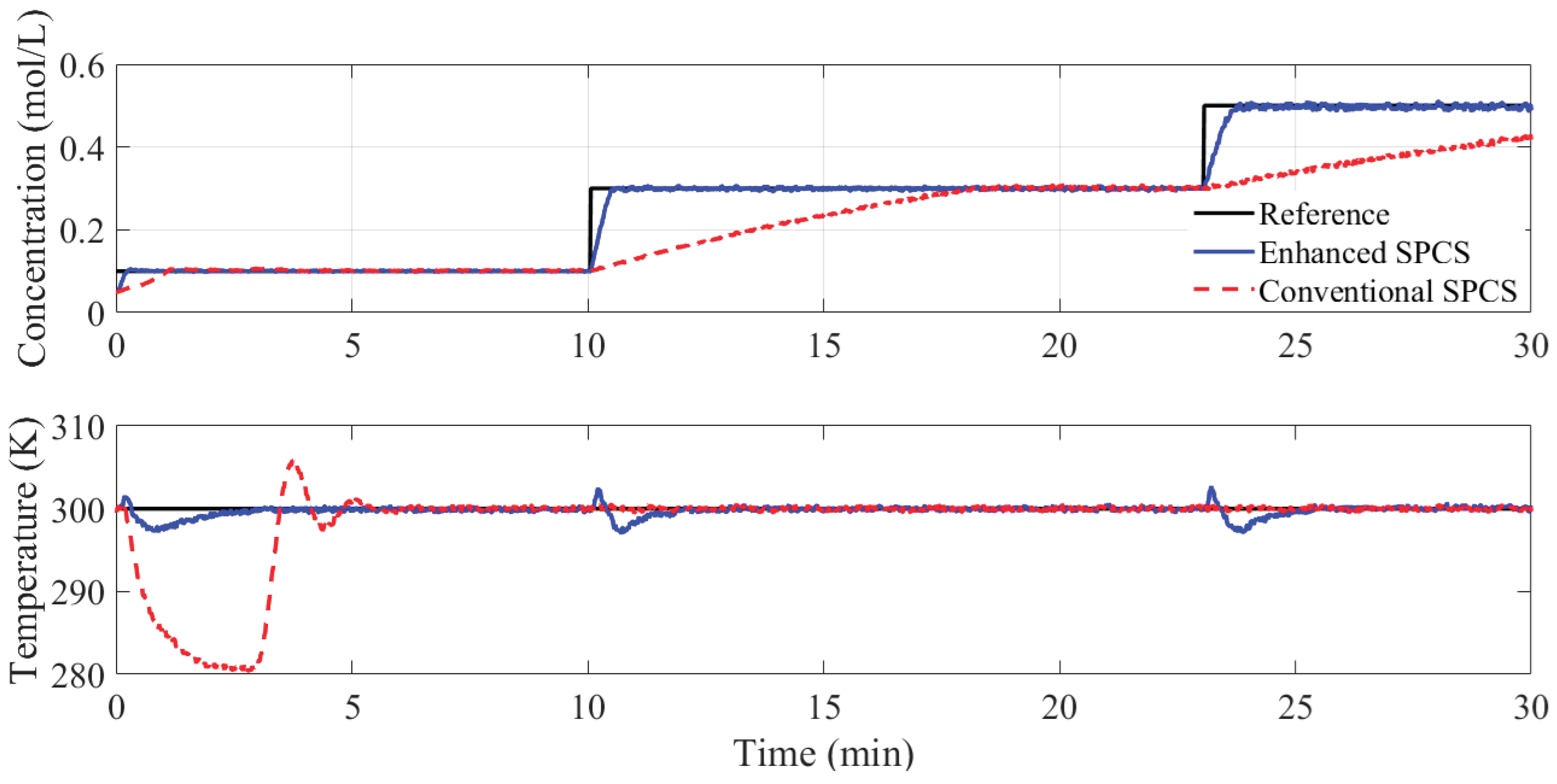
Figure 4 and Figure 5 compare the simulation results of the proposed Enhanced SPCS with a conventional SPCS with two arrays of PIDs, four each, carefully turned for delay-less form of transfer functions in (26) and (27), as detailed in the Appendix A. A conventional SPCS was also designed for the case study with PIDs tuned using decentralised and centralised multivariable approaches. However, it failed to exhibit a presentable performance showing the challenging nature of this control problem. The original nonlinear system of (13) has been used in simulations with a sampling frequency of 1Hz, which is easily achievable in practice. The range of auxiliary temperature is [280350] K, and maximum flow rate of valves is 60 L/min. No measurement noise was considered in simulations presented in Figure 4 and Figure 5.
The enhanced SPCS evidently outperforms conventional SPCS with PIDs in concentration control and catches temperature reference much faster. The results also show that changes of concentration reference affect the temperature control for the proposed control system. The reason is that the proposed control system priorities concentration control, as a design requirement, through selection of faster closed loop poles for the concentration. Interestingly, upper graph of Figure 5 shows that the proposed control system uses the capacity of valves in full to compensate the error where the reference changes. The conventional SPCS with PIDs does not use this capacity and is consequently slower. This behaviour is rooted in inherent trade-off in PID design that slows down the system to avoid concentration overshoots. Moreover, the effect of integral windup is evident in bottom graph of Figure 5 as another weak point of the conventional SPCS with PIDs.
Figure 5 also indicates that, in the proposed control system, significant and fast changes of control inputs only happened at the beginning of operation or in the case of a change in the reference; while, conventional SPCS with PIDs turns water/feed valves ON/OFF very frequently e.g. in time periods of 3-10 minutes and 18-23 minutes and struggles to maintain the concentration on the reference, after it is reached. This is a great advantage for the proposed enhanced SPCS in terms of implementation and energy consumption. This advantage is influenced by the feedforward component of the enhanced SPCS. In order to elucidate such an influence, it should be noted that the CSTR (like many other processes) matches with the definition of generalised type zero (GTZ) systems proposed in [50]. In a GTZ system, the control equilibrium point (CEP) of the system is maintained only by continuous exertion of a control input; CEP is the situation where the error and its derivatives are zero [51]. The feedforward component in (8), detailed in (25) for the case study, has been designed to maintain the desired status of (10), when it is reached. The desired status equals CEP in the case study of this paper as detailed in section 3-2. In the absence of such a feedforward component in the control systems merely relying feedback PID controllers, when the reference is reached, the control input drops to zero shortly, which cannot keep a GTZ on the reference, this leads to the rise of error and a jump in control input to compensate it, e.g. the jumps in the middle graph of Figure 5.
The area outlined with an ellipse in Figure 5 shows the effect of Enhancement 2, where output of the Smith predictors is compared with its asynchronous value of reference in the future to produce the predicted error; please be notes that the reference changes at 10.05 minutes or 10 minutes and 3 second, not exactly at 10 min. The predicted error is fed to (20)/(21) for a timely action and improved performance.
6. Conclusions
In this paper, first, two shortcomings of conventional Smith-Predictor-based control systems were identified: (i) use of classical feedback controllers with their inherent constraints and (ii) asynchrony between the reference and the predicted output. The latter particularly causes the response to have a lag in tracking the reference. On this basis, two enhancements were proposed for SPCSs designed for MIMO time-delay systems: (i) replacing the array of classical feedback controllers by a feedback-feedforward arrangement, and (ii) supplying some future reference value(s) upfront to the control system. Section 2 demonstrates the proposed control system in detail.
The proposed enhanced SPCS was examined to control a nonlinear exothermic MIMO CSTR with multiple time delays and outperformed a conventional SPCS with PID feedback controllers manifestly. The employed CSTR model includes unprecedented level of details and comprehensiveness in terms of inputs, outputs, time-delays, actuators’ limits and sensor noises to assure that the proposed results are realistic, and the proposed method is implementable. The proposed method not only presented an excellent tracking performance; but also, it witnessed much fewer undesirable rapid changes of control inputs.
Acknowledgments
Research resulted in this paper was supported by German University of Technology in Oman, through Seed Grant #SG2025/NR/ENG/MM.
Nomenclature
| Abbreviations | Vectors and Matrices | ||
| BW | bandwidth | A | system matrix |
| CEP | control equilibrium point | B | input matrix |
| CSTR | catalytic stirred tank reactor | C | output matrix |
| GTZ | generalised type zero | K | controller gain matrix |
| MIMO | multi-input multi-output | U | control input vector |
| PID | proportional integral derivative | X | state vector |
| PM | phase margin | Y | output vector |
| SISO | single-input single-output | ||
| Latin Letters | Subscripts | ||
| c | specific heat coefficient [g/(L.K)] | A | effluent |
| C | concentration [mol/L] | d | desired |
| C(s) | controller transfer function | f | feed |
| G(s) | plant transfer function | i,j | index |
| e | control error | p | predicted |
| E | Arrhenius activation energy [J/ mol] | s | sampling |
| H | heat of reaction [J/ min] | u | related to input |
| k | counting index | w | water |
| n | number | x | auxiliary |
| P | pole | y | related to output |
| q | flow rate [L/min] | ||
| r | discrete delay | Superscripts | |
| R | gas constant [J/(mol.K)] | * | related to the desired status |
| s | Laplace variable | ^ | approximated |
| t | time/ time delay without/with an index | ||
| T | temperature [K] | Greek Letters | |
| u | control input | β | gain of a first order transfer function |
| V | reactor volume [L] | κ | reaction velocity constant [min-1] |
| x | system state | ρ | density [g/L] |
| y | output | τ | time constant of a first order transfer function |
| z | Z-transform variable | ι | index |
Appendix A. PID Tuning for Conventional SPCS
pidtune command of MATLAB Control System Toolbox, version 24.2, was used in this research to tune PIDs for conventional SPCS of (5) [54], where centralised and decentralized MIMO tuning of PIDs practically failed. The PID of C(s) is tuned for the plant of G(s):
In the employed algorithm, a target crossover frequency, ωc, and PID controller parameters, are defined so that the condition (29) is met and (non-constant) suitable bandwidth, BW in (32), maximum sensitivity in (31) and phase margine, PM in (30), are obtained based on plant dynamics through an iterative algorithm.
References
- X. Li, W. Liu, S. Gorbachev, and J. Cao, "Event-triggered impulsive control for input-to-state stabilization of nonlinear time-delay systems," IEEE Transactions on Cybernetics, vol. 54, no. 4, pp. 2536-2544, 2023. [CrossRef]
- S. Sharma and P. K. Padhy, "An indirect approach for online identification of continuous time-delay systems," International Journal of Numerical Modelling: Electronic Networks, Devices and Fields, vol. 35, no. 1, p. e2947, 2022. [CrossRef]
- M. Huba, P. Bistak, D. Vrancic, and M. Sun, "PID vs. Model-Based Control for the Double Integrator Plus Dead-Time Model: Noise Attenuation and Robustness Aspects," Mathematics, vol. 13, no. 4, p. 664, 2025. [CrossRef]
- P. Sharma and S. Neeli, "A systematic review of discretisation methods for time-delay systems," Journal of Control and Decision, vol. 12, no. 3, pp. 335-350, 2025. [CrossRef]
- A. Abdusalomov, S. Khusanov, I. Ibragimov, J. Sevinov, M. Mukhiddinov, and Y. I. Cho, "Adaptive Discrete Control of a Rotary Dryer with Time Delay in Potash Fertilizer Production," Processes, vol. 14, no. 5, p. 871, 2026. [CrossRef]
- Z.-G. Liu, Z.-W. Jiang, W. Sun, and S.-F. Su, "Decentralized Tracking Control of Large-Scale Time-Delay Nonlinear Systems and Application to Chemical Reactor System," IEEE Transactions on Systems, Man, and Cybernetics: Systems, 2025. [CrossRef]
- P.-L. Liu, "Further results on delay-range-dependent stability with additive time-varying delay systems," ISA Transactions, vol. 53, no. 2, pp. 258-266, 2014. [CrossRef]
- J. M. Araújo and T. L. M. Santos, "Control of a class of second-order linear vibrating systems with time-delay: Smith predictor approach," Mechanical Systems and Signal Processing, vol. 108, pp. 173-187, 2018. [CrossRef]
- R. J. Vazquez Guerra, J. F. Marquez Rubio, and B. del Muro-Cúellar, "Design of delayed PID-type controllers for high-order recycling systems with time delays using model reduction," Asia-Pacific Journal of Chemical Engineering, vol. 16, no. 4, pp. 1-16, 2021. [CrossRef]
- V. L. Korupu and M. Muthukumarasamy, "A comparative study of various Smith predictor configurations for industrial delay processes," Chemical Product Process Modeling, 2021. [CrossRef]
- M. Mohammadzaheri and M. Ghodsi, "An Enhanced Smith-Predictor-based Control System for delayed MIMO Processes and its Use on a CSTR with Multiple Time-delays," in 2023 28th International Conference on Automation and Computing (ICAC), 2023: IEEE, pp. 1-6.
- H. Chen, Q. Li, Z. Ye, and S. Pang, "Neural Network-Based Parameter Estimation and Compensation Control for Time-Delay Servo System of Aeroengine," Aerospace, vol. 12, no. 1, p. 64, 2025. [CrossRef]
- P. Kumari, P. Kumar, M. H. Ali, G. Manikanta, A. K. Pandey, and A. K. Saha, "Nonlinear Active Disturbance Rejection Control for Unstable Processes With Time Delay: A Case Study of a Continuous Stirred Tank Reactor," Results in Engineering, p. 110296, 2026. [CrossRef]
- X. Li and C. E. deSouza, "Delay-dependent robust stability and stabilization of uncertain linear delay systems: A linear matrix inequality approach," (in English), IEEE Trans. Autom. Control, Article vol. 42, no. 8, pp. 1144-1148, Aug 1997. [Online]. Available: <Go to ISI>://WOS:A1997XP92300010. [CrossRef]
- K.-C. Ri, Y.-I. Kim, and S.-J. Ri, "Robust fault-tolerant control and application in DCS with uncertainty and time delay," International Journal of Dynamics and Control, vol. 13, no. 2, p. 44, 2025. [CrossRef]
- M. Mohammadzaheri and R. Tafreshi, "An enhanced Smith predictor based control system using feedback-feedforward structure for time-delay processes," The Journal of Engineering Research [TJER], vol. 14, no. 2, pp. 156-165, 2017. [CrossRef]
- M. Wu, Y. He, and J. H. She, Stability analysis and robust control of time-delay systems. Springer, 2010.
- Y.-L. Zhi, X. Liu, S. He, W. Lin, and W. Chen, "Adaptively Event-Triggered $ H\infty $ Control for Networked Autonomous Aerial Vehicles Control Systems Under Deception Attacks," IEEE Transactions on Industrial Informatics, 2025. [CrossRef]
- Q. C. Zhong, Robust control of time-delay systems (no. 2009). Springer, 2006.
- J. Cai, D. Guo, and W. Wang, "Adaptive fault-tolerant control of uncertain systems with unknown actuator failures and input delay," Measurement and Control, vol. 58, no. 7, pp. 923-934, 2025. [CrossRef]
- K. Divakar, M. P. Kumar, C. Dhanamjayulu, and G. Gokulakrishnan, "A Technical Review on IMC-PID Design for Integrating Process With Dead Time," IEEE Access, 2024. [CrossRef]
- B. W. Bequette, Process Control: Modeling, Design, and Simulation, 2nd Edition. Prentice Hall Professional, 2023.
- M. Mohammadzahri, A. Khaleghifar, M. Ghodsi, P. Soltani, and S. AlSulti, "A Discrete Approach to Feedback Linearization, Yaw Control of An Unmanned Helicopter," Unmanned Systems, pp. 1-10, 2022. [CrossRef]
- M. Mohammadzaheri et al., "Digital Model-Based Motor Servo Control Considering a Sampling-Induced Time Delay," in 12th International Conference on Control, Dynamic Systems, and Robotics, CDSR 2025, 2025: Avestia Publishing, p. 9.
- K. Perev, "Feedback control for plants with time delay," in IOP Conference Series: Materials Science and Engineering, 2024, vol. 1317, no. 1: IOP Publishing, p. 012002.
- O. J. Smith, "Closer control of loops with dead time," Chemical Engineering Progress, vol. 53, no. 5, pp. 217-219, 1957.
- T. L. Santos, R. C. Flesch, and J. E. Normey-Rico, "On the filtered Smith predictor for MIMO processes with multiple time delays," Journal of Process Control, vol. 24, no. 4, pp. 383-400, 2014. [CrossRef]
- R. Azarmi, A. K. Sedigh, M. Tavakoli-Kakhki, and A. Fatehi, "Design and implementation of smith predictor based fractional order PID controller on MIMO flow-level plant," in 23rd Iranian Conference on Electrical Engineering 2015: IEEE, pp. 858-863.
- T. Dogruer, "Design of I-PD controller based modified smith predictor for processes with inverse response and time delay using equilibrium optimizer," IEEE Access, vol. 11, pp. 14636-14646, 2023. [CrossRef]
- K. J. Astrom, C. C. Hang, and B. Lim, "A new Smith predictor for controlling a process with an integrator and long dead-time," IEEE Trans. Autom. Control, vol. 39, no. 2, pp. 343-345, 1994. [CrossRef]
- A. Mehallel and V. Feliu-Batlle, "Reduction of the Disturbance Effects in a Twin Rotor Multi-Input Multi-Output System Based on a Modified Smith Predictor Control Scheme," Applied Sciences, vol. 15, no. 10, p. 5499, 2025. [CrossRef]
- A. DePoar, "A modified Smith predictor and controller for unstable processes with time delay," Int. J. Control, vol. 41, no. 4, pp. 1025-1036, 1985. [CrossRef]
- P. Albertos, X. Luan, and P. Garcia, "Smith predictor based control of multi time-delay processes," Annual Reviews in Control, vol. 60, p. 101008, 2025.
- B. Ebrahimi, R. Tafreshi, J. Mohammadpour, M. Franchek, K. Grigoriadis, and H. Masudi, "Second-Order Sliding Mode Strategy for Air--Fuel Ratio Control of Lean-Burn SI Engines," IEEE Transactions on Control System Technology vol. 22, no. 4, pp. 1374-1384, 2014. [CrossRef]
- B. Ebrahimi, R. Tafreshi, M. Franchek, K. Grigoriadis, and J. Mohammadpour, "A dynamic feedback control strategy for control loops with time-varying delay," (in English), Int. J. Control, Article vol. 87, no. 5, pp. 887-897, May 2014, doi: 10.1080/00207179.2013.861612. [CrossRef]
- B. Ogunnaike and W. Ray, "Multivariable controller design for linear systems having multiple time delays," AIChE Journal, vol. 25, no. 6, pp. 1043-1057, 1979. [CrossRef]
- I. M. Pataro, M. V. A. da Costa, and B. Joseph, "Advanced Simulation and Analysis of MIMO Dead Time Compensator and Predictive Controller for Ethanol Distillation Process," IFAC-PapersOnLine, vol. 52, no. 1, pp. 160-165, 2019. [CrossRef]
- P. Aryan, M. Mohammadzaheri, L. Chen, M. Ghanbari, and A. Mirsepahi, "GA-IMC based PID control design for an infrared dryer," presented at the Chemeca Adelaide, South Australia, 26-29 September, 2010.
- F. Asadi, State-space control systems: The MATLAB®/simulink® approach. Springer Nature, 2022.
- J. Na, X. Ren, C. Shang, and Y. Guo, "Adaptive neural network predictive control for nonlinear pure feedback systems with input delay," Journal of Process Control, vol. 22, no. 1, pp. 194-206, 2012. [CrossRef]
- M. Mohammadzaheri and L. Chen, "Double-command feedforward-feedback control of a nonlinear plant," (in English), Korean J. Chem. Eng., Article vol. 27, no. 5, pp. 1372-1376, Sep 2010, doi: 10.1007/s11814-010-0258-8. [CrossRef]
- P. B. Sistu and B. Wayne Bequette, "A comparison of nonlinear control techniques for continuous stirred tank reactors," Chemical engineering science, vol. 47, no. 9, pp. 2553-2558, 1992. [CrossRef]
- J. Alvarez-Ramirez and R. Femat, "Robust PI stabilization of a class of chemical reactors," Systems & control letters, vol. 38, no. 4, pp. 219-225, 1999. [CrossRef]
- V. Ghaffari, S. V. Naghavi, and A. Safavi, "Robust model predictive control of a class of uncertain nonlinear systems with application to typical CSTR problems," Journal of Process Control, vol. 23, no. 4, pp. 493-499, 2013. [CrossRef]
- S. Kuntanapreeda and P. M. Marusak, "Nonlinear extended output feedback control for CSTRs with van de Vusse reaction," Computers & Chemical Engineering, vol. 41, pp. 10-23, 2012. [CrossRef]
- M. Mohammadzaheri and L. Chen, "Double-command fuzzy control of a nonlinear CSTR," Korean journal of chemical engineering, vol. 27, no. 1, pp. 19-31, 2010.
- M. Pérez and P. Albertos, "Self-oscillating and chaotic behaviour of a PI-controlled CSTR with control valve saturation," Journal of Process Control, vol. 14, no. 1, pp. 51-59, 2004. [CrossRef]
- P. Sukkarnkha and C. Panjapornpon, "Input/output linearization with a two-degree-of-freedom scheme for uncertain nonlinear processes," Korean J. Chem. Eng., vol. 29, no. 6, pp. 716-723, 2012. [CrossRef]
- B. ZareNezhad and A. Aminian, "Application of the neural network-based model predictive controllers in nonlinear industrial systems. Case study," Journal of the University of Chemical Technology and Metallurgy, vol. 46, no. 1, pp. 67-74, 2011.
- M. Mohammadzaheri, L. Chen, A. Mirsepahi, M. Ghanbari, and R. Tafreshi, "Neuro-Predictive Control of an Infrared Dryer with a Feedforward-Feedback Approach," Asian Journal of Control, vol. 17, no. 5, pp. 1972-1977, 2015/9/1 2015. [CrossRef]
- M. Mohammadzaheri and L. Chen, "Design and stability discussion of an hybrid intelligent controller for an unordinary system," Asian Journal of Control, vol. 11, no. 5, pp. 476-488, 2009. [CrossRef]
- A. N. Pearce J., Bojkovski J., Edler F., de Groot M., Izquierdo G.G., Kalemci M., Strnad R., "Guidelines on the Calibration of Thermocouples," Good Practice Guide 2020. [Online]. Available: https://www.euramet.org/publications-media-centre/calibration-guidelines/.
- G. Gorla, J. A. Iturrioz, K. H. Esbensen, and J. M. Amigo, "Getting “sampling” right for reliable process monitoring: main challenges and solutions," Frontiers in Analytical Science, vol. 6, p. 1839552, 2026. [CrossRef]
- MathWorks. "pidtune." https://www.mathworks.com/help/control/ref/dynamicsystem.pidtune.html (accessed.
Figure 1.
Schematics of a conventional Smith-predictor-based control system in Laplace domain.
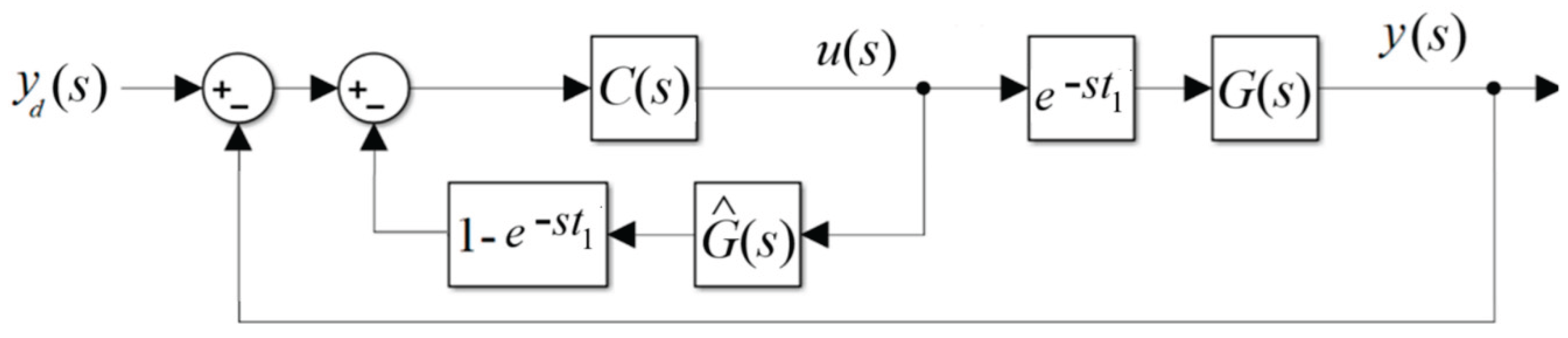
Figure 2.
A re-arranged presentation of Figure 1.
Figure 2.
A re-arranged presentation of Figure 1.
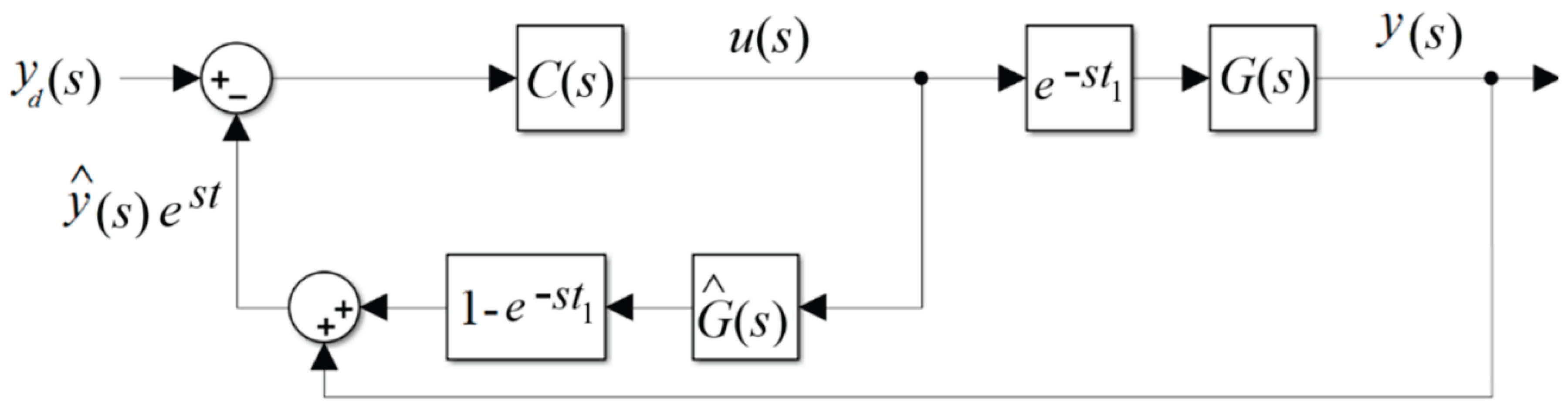
Figure 3.
An enhanced smith-predictor-based control system for a SISO problem.
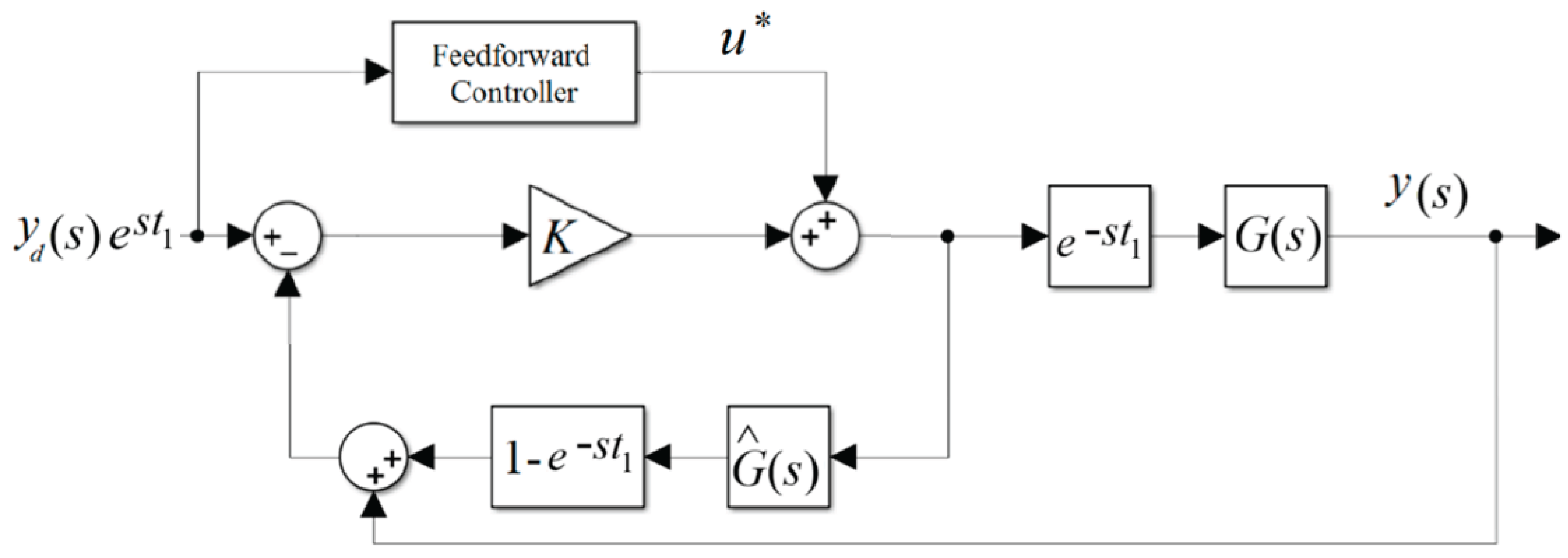
Figure 4.
Control outputs for conventional SPCS with PIDs and the enhanced SPCS without noise.
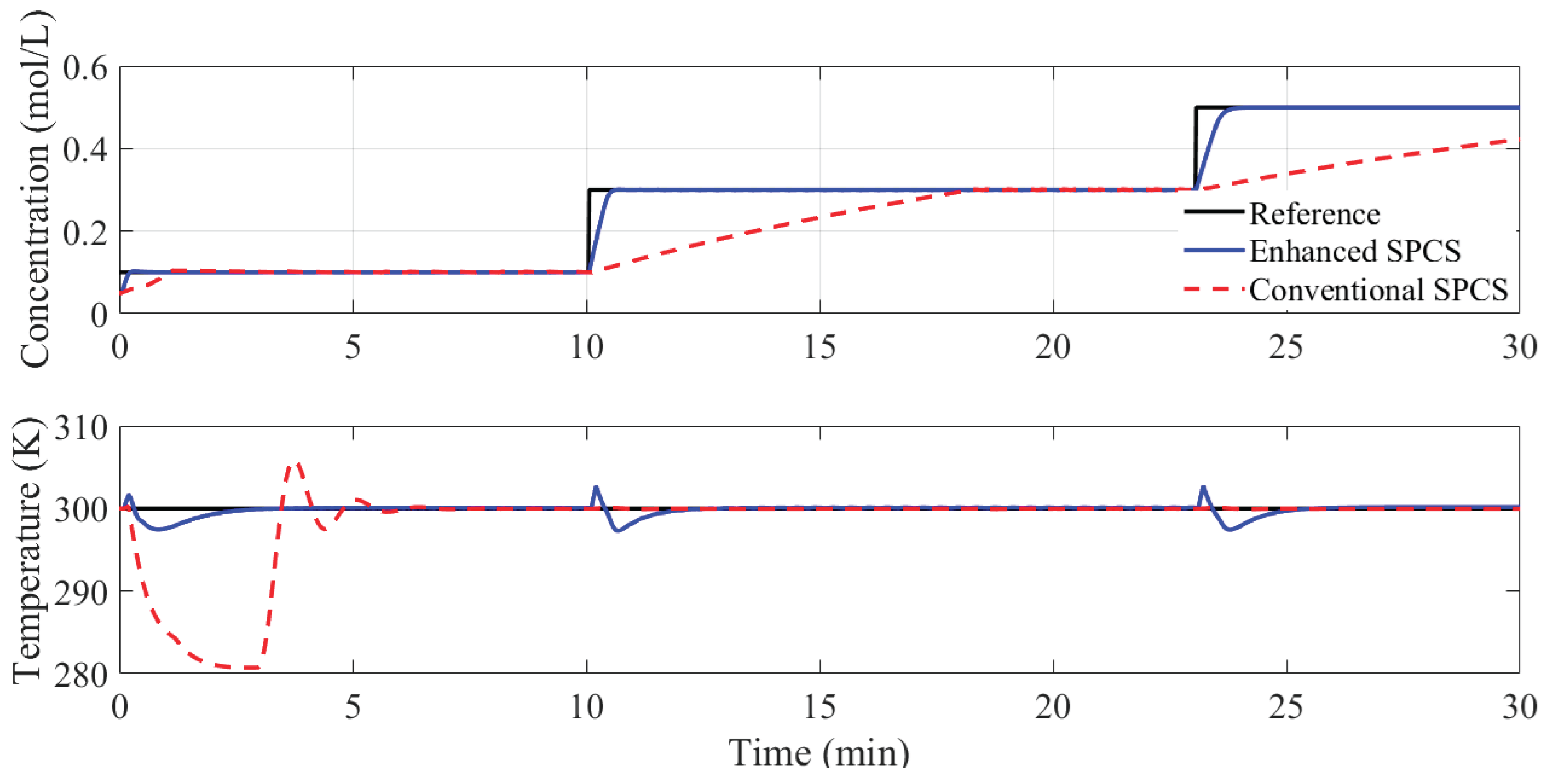
Figure 5.
Control inputs for conventional SPCS with PIDs and enhanced SPCS without noise, related to control outputs presented in Figure 4.
Figure 5.
Control inputs for conventional SPCS with PIDs and enhanced SPCS without noise, related to control outputs presented in Figure 4.
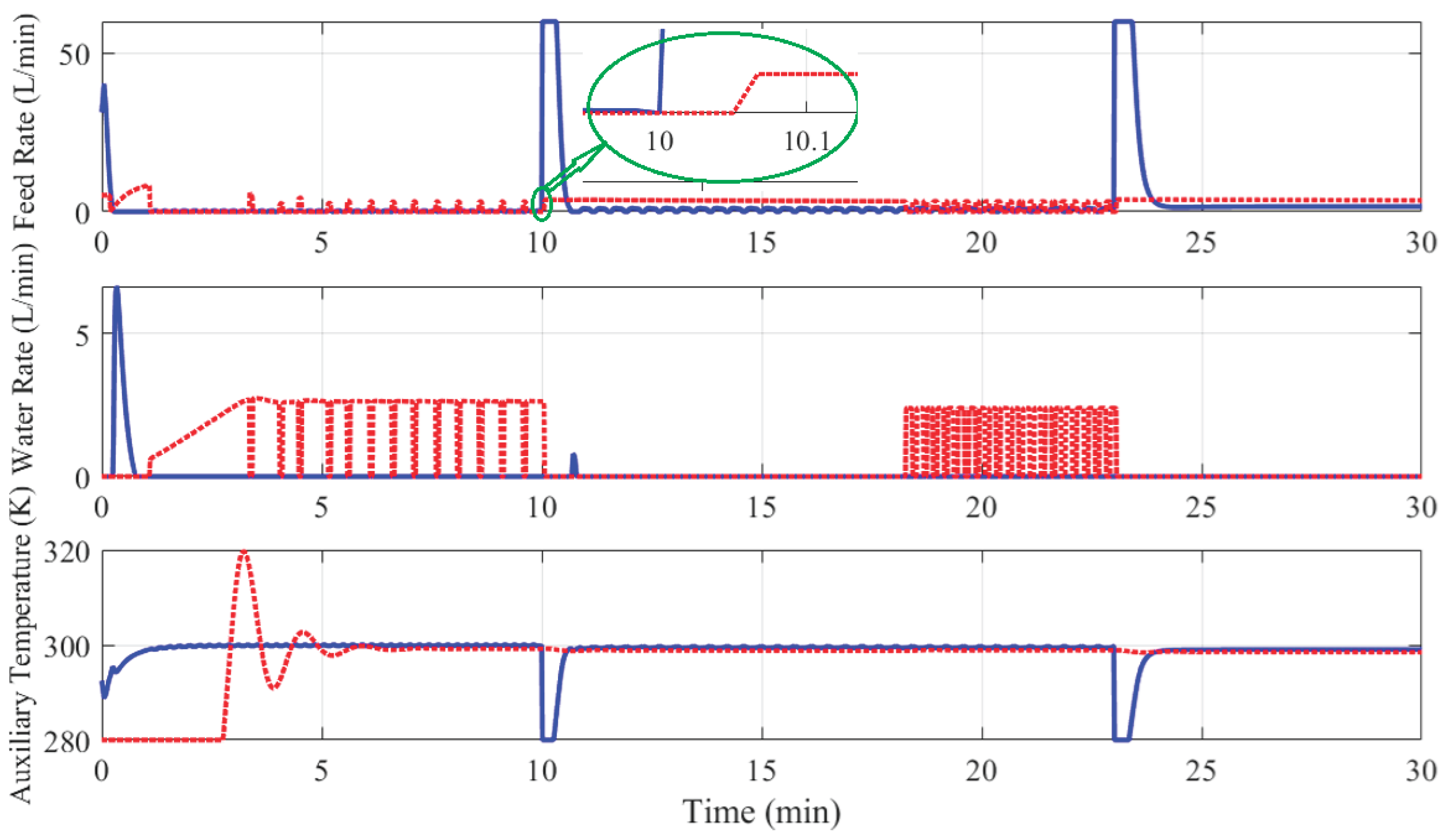
Figure 6.
Simulations results with the proposed control system and conventional SPCS with PIDs. Noises are added.
Figure 6.
Simulations results with the proposed control system and conventional SPCS with PIDs. Noises are added.
Disclaimer/Publisher’s Note: The statements, opinions and data contained in all publications are solely those of the individual author(s) and contributor(s) and not of MDPI and/or the editor(s). MDPI and/or the editor(s) disclaim responsibility for any injury to people or property resulting from any ideas, methods, instructions or products referred to in the content. |
© 2026 by the authors. Licensee MDPI, Basel, Switzerland. This article is an open access article distributed under the terms and conditions of the Creative Commons Attribution (CC BY) license (http://creativecommons.org/licenses/by/4.0/).
Copyright: This open access article is published under a Creative Commons CC BY 4.0 license, which permit the free download, distribution, and reuse, provided that the author and preprint are cited in any reuse.


