
Submitted:
29 July 2026
Posted:
30 July 2026
You are already at the latest version
Abstract
A lattice Boltzmann model (LBM) was developed for thermal radiation transfer in atmospheric aerosol medium. The basic principle and computation procedure of LBM of radiation transfer in aerosol medium were described in this article. A new normalization method for the aerosol scattering phase function was described following the recent literature. The LBM results were validated by comparing the outputs from a Monte Carlo model (MCM) with same boundary conditions and aerosol property parameters. Two cases of validation with beam and diffused incoming radiation boundaries were simulated with both LBM and MCM. The spheric participation medium was assumed in which a Henyey-Greenstein Mie scattering phase function was used. The third LBM result was also compared with the MCM results in the situation of partial cloudy and clear atmospheric media in the domain. All three validations cases indicated that the LBM gives accurate results compared with the traditional MCM in atmospheric aerosol media, the root square difference between the LBM and MCM results were less than 0.03 for normalized unit incoming radiative intensity. The LBM was successfully implemented on a GPU to speed up the computation and reduce energy consumption. The test results indicated that CPU/GPU computation time ratio was around 260 for a 5013 grids computational domain, indicating a significant GPU computational advantage of the LBM for radiation transfer in aerosol medium.
Keywords:
lattice Boltzmann model
; radiation energy transfer modeling in aerosol medium
; aerosol scattering
; Mie scattering
; GPU computing
1. Introduction
The aerosols are abundant in the troposphere, especially in the atmospheric boundary layer. They are either generated from natural processes (dust, sea salt, fog, cloud) or from human activities (smoke, smog, and other air pollutants). Since the aerosols are effective radiative scatter, they play an important role in atmospheric radiative energy transfer. The aerosol particle sizes are much larger than the air molecules, usually in the range of a few wavelengths of visible light to several micrometers, and the light interaction with aerosol does not follow the isotropic Rayleigh scattering law of molecular scattering. The scattering of light by aerosols is highly anisotropic and concentrated in forward or backward directions, depending on the properties and morphology of aerosols. Accurate modeling of radiation transfer in the aerosol medium is important in analysis of natural radiative energy transfer processes in atmosphere, light signal propagation, directed energy transfer, and remote sensing of atmospheric environment.
The radiative transfer process can be modeled using radiative transfer equation (RTE). Since analytical solutions are possible only for simplest, idealized conditions, different computation methods, such as discrete ordinate method (DOM) [1,2,3], finite volume method [4,5], and Monte Carlo method (MCM) [6] have been developed to solve the RTE numerically. All those numerical methods of solving RTE demand a large amount of computation time. MCM is often used as a benchmark method to validate the numerical solution of other methods. Although MCM is accurate and versatile in solving the RTE, it demands most intensive computing compared with other methods. As computation domain is getting larger or resolution of grid is finer, computation intensity grows rapidly.
An accurate and computationally efficient method is desired for modeling radiative energy transfer in the atmosphere. During recent years, great progress has been made in developing lattice Boltzmann method (LBM) for rapid computation of radiative energy transfer problems. The LBM was first discovered and developed in the fluid mechanics community [7,8,9,10,11,12,13,14,15,16] and has become one of the most effective methods in terms accuracy and computation speed for fluid flow and heat transfer simulations. LBM is based on the kinetic theory of statistical mechanics and solves the Boltzmann equation that governs the probability distribution of fluid particles. The LBM solves the Boltzmann equation for a particle at each grid point by performing collision and propagation calculations of the particle’s probability distribution function (PDF) over a discrete and symmetric lattice mesh with certain fixed directions. The macroscopic variables of fluid flow, such as u,v,w, can be derived from the statistical moments of PDF solved by LBM. The LBM flow models, implemented on a GPU computation platform, can drastically increase computation speed by about 300 times [16] compared with a CPU implementation. The LBM algorithm is well suited on GPU because LBM calculations are highly localized, data parallel. A particle collision and streaming steps in LBM only use information from its immediate neighbor grids. The RTE equation comprises terms of energy advection (propagation) and diffusion (scattering/absorption), it is natural to explore the LBM as a computational method to accelerate the computation speed in modeling radiative transfer. The LBM can be considered a direct discretization of the Boltzmann equation [7]. Because of the similarity between the RTE and Boltzmann equation [17], earlier research and development of the LBM for the RTE started with direct discretization of the RTE with respect to space, time, and angular direction. The earliest work of solving the RTE using the LBM by Giest et al. [18] was for rendering computer graphics considering the radiation effects. Asinari et al. and Mishra et al. [19,20] developed a two-dimensional (2-D) LBM for radiative transfer modeling in a particular medium. Ma et al. [21] derived an LBM used for a one-dimensional (1-D) radiation problem that compared well with an analytical solution. Bindra and Patil [22] and McCulloch and Bindra [23] also developed a 2-D LBM for the RTE for a simulation of the conjugated radiative and convective heat transfer problem. A general review on modeling neutron and photon transport using LBM is provided in [24]. The LBM was also used in a non-equilibrium radiation transfer problem [25]. Zhang et al. [26] and Yi et al. [27] derived a 2-D LBM using the Chapman–Enskog expansion for a steady-state radiative transfer problem that can deal with both thin and high optical depths. For better treatment of the radiation source term, a multi-relaxation time LBM was developed by Liu et al. [28]. Liu et al. [29] also developed an unstructured grid method in LBM for speed up computation and easier treatment boundary in a homogeneous medium. McHardy et al. [30,31] developed a 3-D LBM model using a direct discretization of the RTE and the model produced accurate results for the ballistic radiation condition in which the medium scattering albedo is less than 0.7. Mink et al. [32,33] developed a 3-D LBM method for high optical thickness situations based on the Chapman–Enskog expansion and a steady-state RTE was approximated by the Helmholtz equation and solved with the LBM. Wang et al. [34] developed a GPU accelerated LBM model for radiation transfer in clean atmosphere with molecular scattering and the great speed acceleration was realized.
Radiative transfer modeling in different aerosol mediums is more complex and less developed compared with its counterparts of radiative transfer in atmospheric molecules. One aspect of difficulty is that radiative parameters for different species of aerosols are not well understood and much more related to material properties and morphology of the aerosols. Another aspect of difficulty is the computation of the radiation transfer process due to the asymmetry scattering parameters. An LBM was developed by McHardy et al. [30] for case of Mie scattering and the results compared well with the MCM. The key signature in solving RTE using LBM for anisotropic scattering aerosol medium is that an anisotropic scattering function (SPF) must be applied in each computation grid. For anisotropic aerosol scattering of larger aerosol particles, the SPF is not uniform and must be specified with incoming angles. Furthermore, the SPE must be normalized to obey the energy conservation in the system [3,30,35,36] . SPE of aerosols can be derived from theoretical analysis of solutions of the Maxwell equations [37,38,39] or laboratory observations [40,41].
The objective of this research is to develop and validate a radiation transfer lattice Boltzmann model (RTLBM) for atmospheric aerosol medium to speed up the computation. This paper is organized as follows: section 2 describes the basic theory of the radiation transfer and derivation of the RTLBM. Section 3 shows the validation of the RTLBM results with a radiation transfer Monte Carlo model (RTMCM) to test the accuracy of the RTLBM, the results of computation times are compared for different sizes of domains to demonstrate the computation efficiency of which RTLBM is implemented on a GPU platform. The final section summaries this research and conclusion.
2. Methods
2.1. The Lattice Boltzmann Equation for the RTE of Aerosol Medium
The RTE is an energy conservation equation for radiation transfer and can be written in the following form:
where R(x,,t) is the spectral radiance at spatial point x, is a direction vector, c is the speed of light, are the medium absorption and scattering coefficients, respectively. is the spectral radiance of blackbody emission, is the solid angle. Since the scattering from aerosol particles can be treated as monochromatic, the spectral dependency of radiance can be dropped out. The is the SPF to direction from direction . In the case of isotropic molecular scattering medium, But for aerosol medium, the scattering is anisotropic, the scattering phase function is different from uniform, it needs an asymmetry parameter, , to account for the distribution of scattering with respect to scattering angle (see Section 2.2).
In the derivation of the Boltzmann type of radiation transfer equation, the relation between the PDF at a direction i () of a virtual particle crossing a solid angle cross-section and the radiance is expressed as [33]
where are the solid angle weights that correspond to the lattice directions. In this article, lattice model with 26 directions is used and their values are
where the i directions in lattice structure are shown in Figure 1. By neglecting the blackbody emission of the aerosol particles, and substituting the absorption and scattering coefficient with extinction coefficient (or optical depth), , and scattering albedo, α, the RTE is transformed into following Boltzmann type equation:
where , .
To keep the model non-dimensional for the comparisons and applications, the medium’s scattering albedo, α, and optical depth, , both are non-dimensional parameters, are used instead of the coefficients of absorption and scattering. The optical depth can be expressed in a normalized form
where is a modeled normalized physical domain length. The main complexity of solving the RTE is in the scattering integral term, especially in the anisotropic scattering medium. The scattering integral is replaced with discrete form summed over all the lattice directions
where is an equilibrium distribution of photon kinetics of particle collision. is a scattering matrix which represents the probability that a photon is scattered from the i to j direction, are the solid angle weights for the integration. For an isotropic scatter particle such molecules in atmosphere, has a different mechanism in radiative transfer than in fluid flow. The equilibrium is the Maxwell and Boltzmann distribution in fluid modeling, representing the approaching fluid particle equilibrium PDF after the collision; The in radiative transfer, however, represents the equilibrium PDF of photon after scattering by the medium particle.
The Equation (4) can be discretized in time, space, and velocity, the resulting lattice Boltzmann equation is as follows [7]:
where is the discrete lattice velocity in different directions of a lattice:
An alternative explanation and derivation of LBM for radiative transfer problem start with the microscopic Boltzmann transport equation. By using the Chapman-Enskog expansion, the macroscopic RTE equation can be recovered [26,27,28,29]. The Chapman-Enskog expansion analysis is fundamental theory that connects the microscopic particle kinetics to the collective macroscopic transport equations. Detailed description about theory and applications of the LBM in general is referred to monograph [13].
After many time steps of collision and streaming iterations, the solution of the equation approaches a steady solution of error with an error tolerance. The radiation intensity, I(x,t), can be computed from the first order statistical moment of the photon PDF. An intensity of radiation field, is defined as
2.2. Normalization of Aerosol Scattering Phase Functions
The scattering of light waves by spheric particles that are comparable in size to the wavelength of the light is described by Mie theory. The scattered light is more intense in forward or backward directions, and the intensity is dependent on wavelength of the light, property, and size of the particle. To avoid much of the complexity of Mie scattering phase function, an approximate phase function of Henyey-Greenstein (HG) is used. The HG function is expressed as
where is the angle from incoming radiation to scattering direction, is the asymmetry factor. To conserve the scattered energy, the HG scattering phase function needs to be normalized to assure the scattering energy to be conserved with the incoming energy and overall asymmetry factor is unaltered [35,36]:
where the subscripts i and j represent the discrete directions i and j, N=26 of the discrete lattice directions, are the solid angle weights that correspond to the lattice directions. McHardy et al. [30] has used an older version of Hunter and Guo [35], which is more complex and computationally intensive for which solves an under-determined liner system involving many interactions. In this research, we chose a new method developed by Hunter and Guo [36], an explicit system which is much simpler than their previous algorithm. The new algorithm was also tested to its accuracy compared with the older algorithm [36]. The new normalization procedure the forward (f) and backward (b) scattering components was altered according to the following formulas,
This normalization can conserve the scattered energy while simultaneously maintaining the original value of asymmetry factor. Normalization vector parameters are computed as follows :
The new algorithm is based on the notion that strong forward scattering HG phase function is significantly larger than the remaining terms [39], only the large terms of forward or backward (for mainly backward scattering aerosols) are altered for scattering energy conservation. In this study, we only consider the forward scattering aerosols. Figure 2 displays the examples of HG normalization results for the different asymmetry parameters. The results show that only the forward direction is altered in the HG function and other values of other directions are on the non-normalized HG curves.
In many situations, the aerosol particles are not spheric but rather in irregular shapes such as ellipsoids, columns, clusters of smaller particles. The laboratory test [40,41] can provide SPF, for single scattering of an aerosol particle. The T-Matrix method can also be applied for single scattering of irregular shaped aerosol particles . The retrieval of SPF for mixed sized aerosol particles can also be derived from the T-Matrix method [37,38,39]. It is not feasible to compute a multiple scattering of countless aerosol particles. It is also to be emphasized that SPF also needs to be normalized as demonstrated to ensure energy and parameter conservations in the multi-scattering medium.
2.3. Boundary Conditions
Three types of boundary conditions were used in this study. The first type is the beam type radiation, represents radiation was from a specified unit beam radiation with a specified elevation angle. The second type of boundary condition is diffused incoming radiation from a boundary. The third type of boundary condition is a non-emitting black boundary condition allowing the radiation to be absorbed completely when the photo hits the boundary. The fourth type of boundary condition is a periodic boundary condition along the lateral boundary planes, representing the simulation domain is uniform out of the simulation domain. The examples of the boundary conditions can be described as follows in the RTLBM (see Figure 1 for the lattice directions):
where is the radiative intensity at the incoming boundary, and is the sum of all weights in the incoming direction.
The RTMCM used in this study is the same as the one that was used in our previous study. For brevity, interested reader is referred to Wang et al. [34].
3. Results
To evaluate the accuracy of the newly developed LBM model for the radiative transfer in the aerosol medium, MCM results were used for this purpose. MCM [34] was also used for evaluation purposes in previous LBMRT modeling of radiative transfer in the isotropic molecular Rayleigh scattering in the atmosphere. Despite MCM huge computational power requirement, MCMs are used for benchmark validation tools in other types of model developments. We also follow the suit of this practice since the observational data is scarce. Since the radiation transfer in aerosol is mainly in high scattering diffusive regime, we focused the following simulations on high scattering albedo.
3.1. Radiation Transfer Simulations in Aerosol Medium with a Beam Incoming Boundary
In this validation of the LBM model for anisotropic radiation transfer in an aerosol medium. A cubic volume of aerosol medium with specified scattering phase function and optical depth were specified. The optical depth of the aerosol medium is 33.333, and the scattering phase function parameter is 0.85. The top boundary is incoming with beam radiation perpendicular to the top plane the computational domain with normalized unit intensity (Figure 3, left panel), and other boundaries are all assumed to be black and non-emitting.
Figure 3 (right panel) are samples of radiative intensities along the Z at the centerline (X=Y=50 grid) computed with both RTMCM and RTLBM methods. Figure 4 displays a 3D dimensional perspective visualization of the computed radiative intensity. Two vertical plane slices, one is parallel to X axis, and another is parallel to Y axis of the simulation domain are shown in the figure. The left panel is the computational results of RTLBM, and right panel is the results from the RTMCM, respectively. Since the model results are all normalized values, we use the root mean square difference (RMSD) to evaluate the average difference between the RTLBM and RTMC results. The RMSD is 0.0307 between the RTLBM and RTMCM for this case of beaming from top boundary to an aerosol medium.
3.2. Radiation Transfer Simulations in Aerosol Medium with a Diffused Incoming Boundary
In this comparison of radiation transfer simulations using the RTLBM and RTMCM methods, the aerosol medium parameters were exactly same as in case 1 stated in section 3.1. The incoming boundary condition was from west plane, and the radiation was a diffused with in RTLBM (same incoming in lattice direction of 1,7,9,11,13,19,21,23,25 (see Figure 1) . In the RTMCM, radiation was allowed to come on west plane in any direction.
McHardy et al. [30] also has done a simulation using their LBM with same setup as current study. The only difference between their implementation of RTLBM is that they used an older method of normalization in phase scattering function, which is much more complex than our normalization of phase scattering function. Figure 3 (right panel) displays the radiative intensity along the centerlines in X direction at Y=Z=0.5. Two simulations of RTLBM and another simulation with RTMCM are quite close along this sampling line.
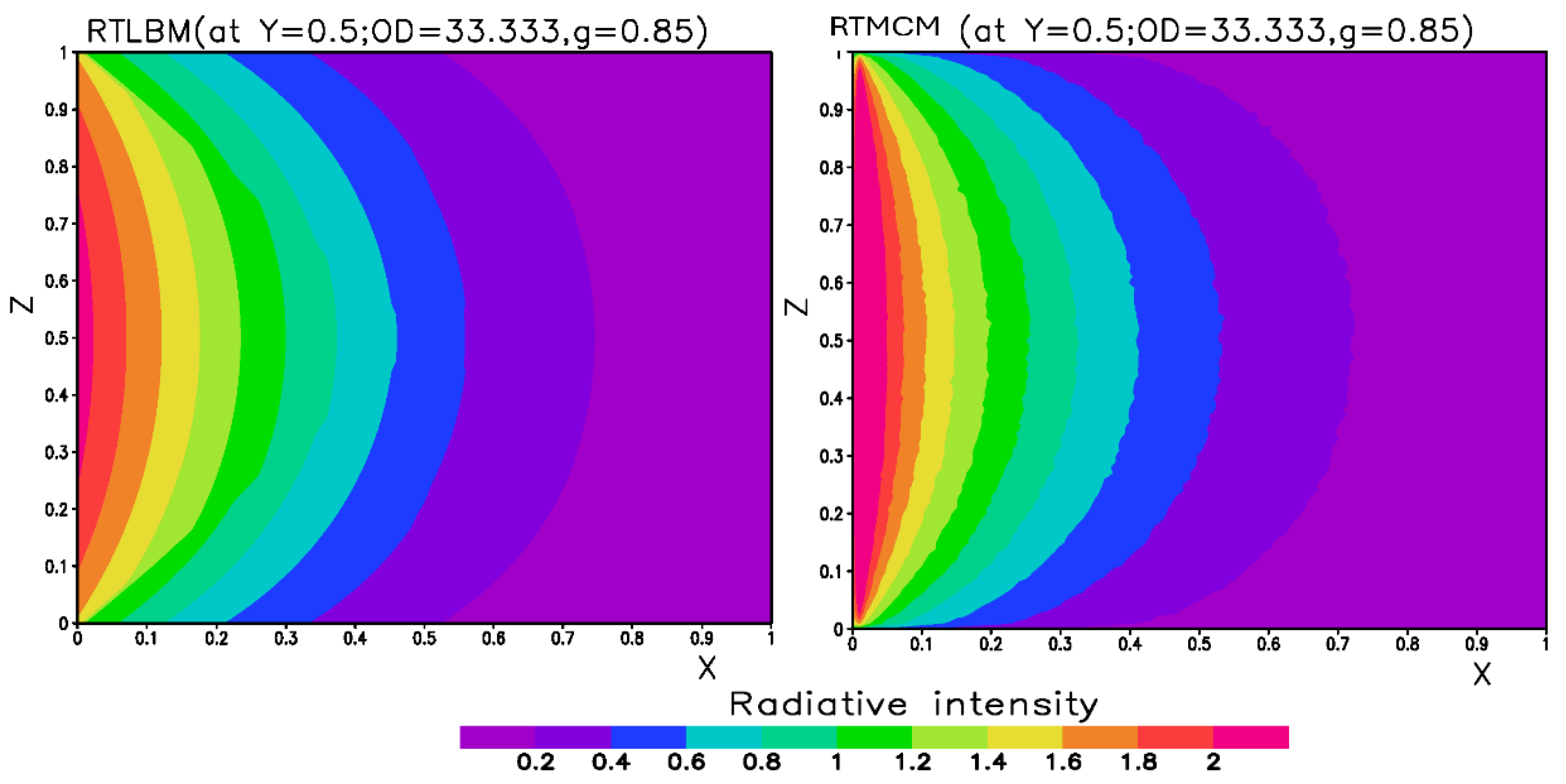
Figure 5 displays vertical cross-sections of RTLBM and RTMCM simulation results of diffused incoming radiation process in an aerosol medium along the X axis at the Y=Z=0.5. The results from both simulations generally agreed reasonably well, but some minor differences near the incoming boundary. The RTMCM result near the incoming boundary had larger radiative intensity than that in the RTLBM simulation result. The differences between the LBM and MC models also showed similar differences, RMSD=0.0145.
Figure 5.
Left panel: a sketch of the 3D computation domain, west diffused income boundary radiation and aerosol medium. Diffuse radiation was from west boundary. Medium aerosol scattering albedo=1, optical depth=33.333, and scattering phase function parameter= 0.85; Right panel: a comparison of center horizontal symmetry line samples (at Y=Z=0.5) of the RTLBM, RTMCM, and McHardy LBM [28] results.
Figure 5.
Left panel: a sketch of the 3D computation domain, west diffused income boundary radiation and aerosol medium. Diffuse radiation was from west boundary. Medium aerosol scattering albedo=1, optical depth=33.333, and scattering phase function parameter= 0.85; Right panel: a comparison of center horizontal symmetry line samples (at Y=Z=0.5) of the RTLBM, RTMCM, and McHardy LBM [28] results.
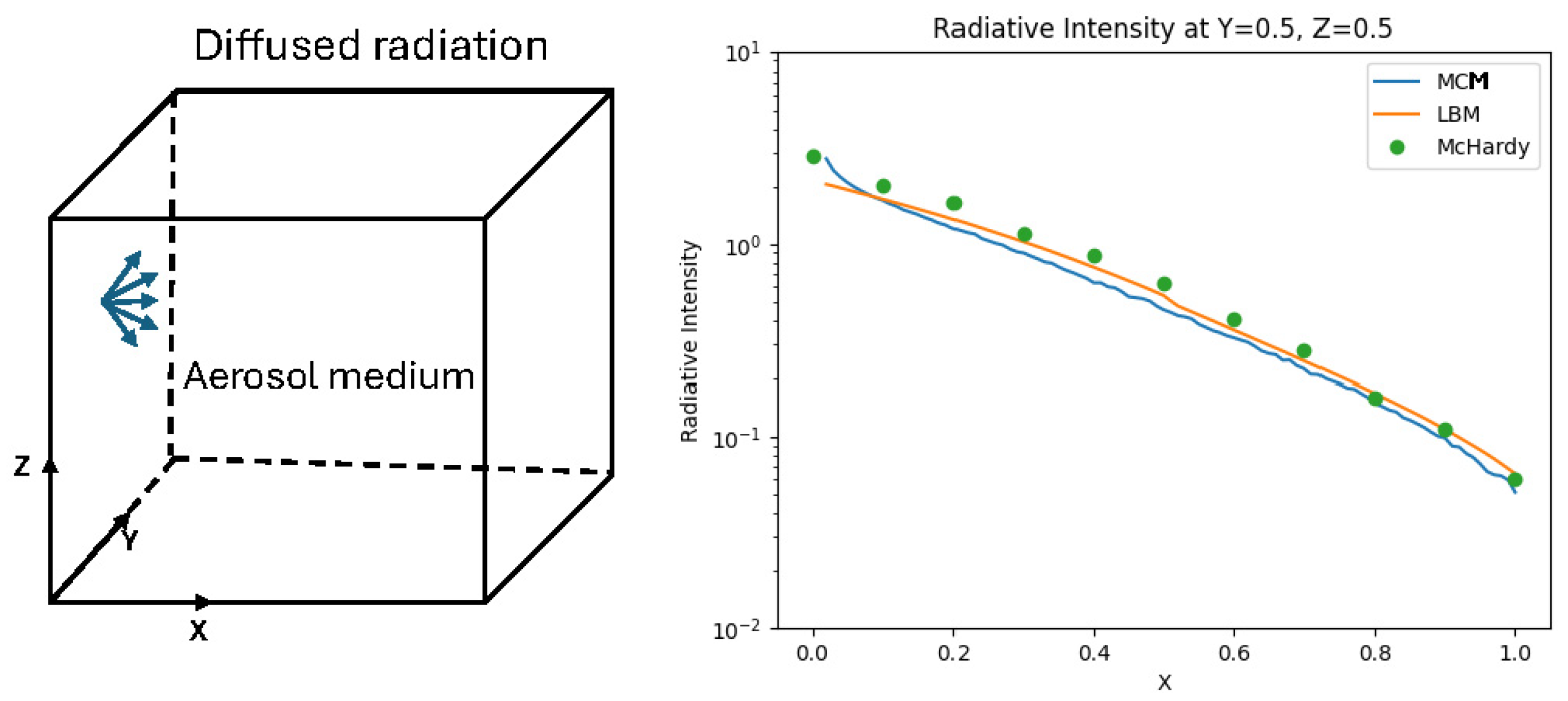
Figure 6.
A side by side comparison of RTLBM and RTMCM results at the center plane cuts (Y=0.5) in the radiative filed. Diffuse radiation was from west boundary. Medium aerosol scattering albeo=1, optical depth=33.333, and scattering phase function parameter= 0.85.
Figure 6.
A side by side comparison of RTLBM and RTMCM results at the center plane cuts (Y=0.5) in the radiative filed. Diffuse radiation was from west boundary. Medium aerosol scattering albeo=1, optical depth=33.333, and scattering phase function parameter= 0.85.
3.3. A Case in Mixed Aerosol and Molecular Scattering Media in the Domain
One of prevalent situations for atmospheric radiation transfer is the clear atmosphere with some cloud coverage or air pollutant in some areas. This is a typical case of mixed media with Mie scattering (cloud occupied volume) and Rayleigh scattering (clean air atmosphere). In this simulation, a typical cumulus cloud area with optical depth of 20 and scattering albedo of 1, and g=0.85 was set up in the volume (x=y=0.45~0.55, z=0.2~0.3). The rest of area has a clear atmosphere with isotropic Rayleigh scattering optical depth of 0.08 and scattering albedo 0.7. The Rayleigh scattering was described in first version of the RTLBM model [34]. The identity flag was set up in the domain for tagging the computation grid occupied by the different scattering medium. The same domain was set up for the RTMCM simulation. Periodic boundary conditions were applied in lateral boundaries.
Figure 7 (left panel) shows a model domain setup as described . Figure 7 (right panel) displays a sample vertical line at center (X=Y=0.5). The RTLBM and the RTMCM produced similar results both in the Rayleigh (clean air) and Mie (cloud) scattering regions in the domain. The RTLBM simulation gave a slightly smaller value of radiative intensity along the vertical line than that of RTMCM simulation, and the location from the peak radiative intensity locations by Mie scattering had some differences. The simulation results from the RTLBM and RTMCM were also cut through the symmetric plane (Y=0.5) and displayed in Figure 8. The radiative intensity showed large values around the cloudy volume. At the cloud shadow area below the cloud showed (Z<0.2) large decrease of radiative intensity. One pattern of radiative ray effect was shown in this LBM simulation. This ray effect error was caused by the limited ray number in the LBM. The ray effect error was also evident in DOM type model due to limited number of rays. This ray effect error is more severe in the case of small and narrow medium cases [30,32]. The overall difference between the RTLBM and RTMCM was evaluated at RMSD value of 0.0210.
3.3. GPU Computation of Radiation Transfer in Aerosol Medium
One of rationale to develop the RTLBM is mainly for its computational speed and reasonably accurate results. The RTMCM model would be the best choice due to its accuracy and versatility in treatment of different types of boundary conditions. However, the RTMCM demands tremendous computational power compared with other methods because the RTMCM samples all the possible directions for billions of the photon transport processes. In all our simulations described in this section with 1013 grids, the computation time for a same single CPU takes approximately 486 times of CPU time using the RTMCM model (6 billion photons) compared with the RTLBM (Table 1). The ratio of computation time (RTMCM/RTLBM) on same CPU is even large if there is a large domain in the computation or more photons are sampled for smoother fields. In the following discussion, we will focus on comparing the computation speed of RTLBM model implemented on the CPU and GPU platforms.
As discussed in the introduction, one of the advantages of the LBM type model is the intrinsic parallelism in the modern GPU platform because the data locality is satisfied and time-stepping is explicit in the LBM algorithm. In the GPU implementation, each computational grid cell in the domain is assigned to a GPU thread. Modern GPU has several thousands of compute cores and are thus able to run thousands of threads simultaneously. The information in the grid is read, processed, and put back in the same memory by this thread. The code uses the Nvidia CUDA® (Common Unified Architecture). The 3D computation grids are mapped to 1D memory, and the data access uses the array structure for memory coalescing. There are many thread blocks in the code, and each thread block does the same computation. Each thread block uses local fast shared memory, avoiding unnecessary local to global memory movement. In GPUs, threads execute in lockstep in sets called warps. The threads within each warp need to load memory together to use the hardware most effectively. This is called memory coalescing. In our implementation, we manage this by ensuring that threads within a warp are accessing consecutive local memory as often as possible. Current version of GPU implementation is in a single GPU processor. We are still in the process of implementing the RTLBM on a multi-GPU computation platform. Here we only report its efficiency for three cases in this paper, as indicated in Table 2. The Tesla A100 GPU (6912 cores, 80 GB memory) has more than 34 times speed-up compared to a CPU (AMD 7713 2 GHz) for a domain size of 1013 grid points. The CPU/GPU computation time ratio increases as the domain size increases, 182 times for a domain of 501*501*301, and 261 times for a domain with 5013 grid points. These results also confirmed that the LBM is a generally memory limited computation algorithm. The LBM with a GPU has shown to be more effective in numerical simulation of turbulent flow in urban environments with at least a 200 to 500 times speed-up (CPU/GPU time ratio) on early generation of the GPU type [14,15].
In the more recent GPU computation, such as AI, it is believed there are more advantages to use the easier Python implementation of the Cuda kernel for better code readability, data flow among the kernels, and rich open graphical and statistical library. The RTLBM is also implemented in Python for this advantage. As shown in Table 2 and Table 3. The speed up factors are quite similar for the C++ and Python implementation.
5. Summary and Conclusions
A fast and reasonable accurate radiative transfer model in atmospheric aerosol medium, RTLBM, was developed using the lattice Boltzmann method. A new normalization algorithm developed by Hunter and Guo [36] was used for application in this model. The RTLBM was evaluated by comparison with results from a Monte Carlo model. The test results indicated that RTLBM is reasonably accurate in the situations of direct beam and diffused incoming boundary conditions with high optical depth and scattering albedo. RTLBM also validated the situation of patch aerosol in the clean atmospheric, emulating the mixed radiation transfer media in Rayleigh and Mie scattering regimes. Like other model methods, such as DOM and FV, the RTLBM also had minor error in the situation of small of narrow patches of media due the relatively a small number of sampling directions. This error can be reduced by dense up the computational grids in the smaller region. The overall quantitate measure of difference between RTLBM with a RTMCM is that RMSD is less than 0.03 for all three test cases.
The motive for developing RTLBM is to develop RTLBM to reduce the massive computation expense compared with other numerical methods. The speedy computation of the RTLBM is based on its special algorithm of streaming and collision. As test results shown, RTLBM can easily be 260 times faster on a GPU (Nvidia A100, not even latest faster B100) than on a CPU, drastically reduced the high computation cost. This test results are comparable to the GPU implement RTLBM [34] of clear atmosphere where scattering is the isotropic Rayleigh regime. This computation speed improvement can significantly reduce the computation burden for modeling the radiative transfer process in complex atmospheric boundary layer such as urban area, where the scattering media and boundaries are complex and highly three dimensional.
Future research and development efforts will be focused on following: (1) application LBM in the plant canopy radiation modeling; (2) different boundaries and two streams (solar and terrestrial) of modeling of urban radiation energy transfer; (3) multi-GPU implementation of the RTLBM for further reduction of computation cost.
Author Contributions
Conceptualization of the RTLBM and study, Y.W.; methodology, and computation and data analysis, Y.W. and X.Z.; GPU and CPU software, J.D. and Y.W.; RTMC model and analysis, X.Z. All authors have read and agreed to the published version of the manuscript.
Funding
This research was funded by US Army DEVCOMARL.
Institutional Review Board Statement
paper was reviewed and approved by the authors’ institution.
Informed Consent Statement
Not applicable.
Data Availability Statement
The data is contained within the article. The model code is currently not available to the general public due to government regulations.
Conflicts of Interest
The authors declare no conflicts of interest.
Abbreviations
The following abbreviations are used in this manuscript:
| CPU | Central processing unit |
| DOM | Discrete ordinate method |
| GPU | Graphical processing unit |
| HG | Henyey-Greenstein |
| LBM | Lattice Boltzmann model |
| MCM | Monte Carlo model |
| Probability distribution function | |
| RTE | Radiative transfer equation |
| RTLBM | Radiative transfer lattice Boltzmann model |
| RTMCM | Radiative transfer Monte Carlo model |
| RMSD | Root mean square difference |
| SPF | Scattering phase function |
References
- S. Chandrasekhar, S. Radiative Transfer; Dover Publications Inc, 1960; p. 393. ISBN 978-0-486-60590-6. [Google Scholar]
- Liou, K.-N. Numerical experiment on Chandrasekhar’s discrete-ordinate method for radiative transfer: Applications to cloudy and Hazy Atmospheres. J. Atmos. Sci. 1973, 7, 1303–1326. [Google Scholar] [CrossRef]
- Hunter, B.; Guo, Z. Comparison of quadrature schemes in DOM for anisotropic scattering radiative transfer. Numer. Heat Transf. Part B CrossRef. 2013, 63, 485–507. [Google Scholar] [CrossRef]
- Chai, J.C.; Lee, H.S.; Patankar, S.V. Finite volume method for radiation heat transfer. J. Thermophys. Heat Transf. CrossRef. 1994, 8, 419–425. [Google Scholar] [CrossRef] [PubMed]
- Coelho, J.P. Advances in the discrete ordinates and finite volume methods for the solution of radiative heat transfer problems in participating media. J. Quant. Spectrosc. Radiat. Transf. CrossRef. 2014, 145, 121–146. [Google Scholar] [CrossRef]
- Howell, J.R. The Monte Carlo method in radiative heat transfer. J. Heat Transf. CrossRef. 1998, 120, 547–560. [Google Scholar] [CrossRef]
- He, X.; Luo, L.-S. Theory of lattice Boltzmann method: From the Boltzmann equation to the lattice Boltzmann equation. Phys. Rev. E CrossRef. 1997, 56, 6811–6817. [Google Scholar] [CrossRef]
- Chai, J.C.; Lee, H.S.; Patankar, S.V. Finite volume method for radiation heat transfer. J. Thermophys. Heat Transf. 1994, 8, 419–425. [Google Scholar] [CrossRef] [PubMed]
- Qian, Y.-H.; d’Humières, D.; Lallemand, P. Lattice BGK models for Navier-Stokes equation. Europhys. Lett. 1992, 17, 479–484. [Google Scholar] [CrossRef]
- Chen, H.; Chen, S.; Matthaeus, W.H. Recovery of the Navier-Stokes equations using a lattice-gas Boltzmann method. Phys. Rev. A 1992, 45, 5339–5342. [Google Scholar] [CrossRef] [PubMed]
- Chen, S.; Doolen, G.D. Lattice Boltzmann method for fluid flows. Annu. Rev. Fluid Mech. CrossRef. 1998, 30, 329–364. [Google Scholar] [CrossRef]
- d’Humières, D.; Ginzburg, I.; Krafczyk, M.; Lallemand, P.; Luo, L.-S. Multiple-relaxation-time lattice Boltzmann models in threedimension. Phil. Trans. R. Soc. Lond. A CrossRef. 2002, 360, 437–451. [Google Scholar] [CrossRef] [PubMed]
- Guo, Z.; Shu, C. Lattice Boltzmann Method and Its Applications in Engineering, Advances in Computational Fluid Dynamics; World Scientific Publishing Co.: Singapore, 2013; Volume 3, ISBN 978-981-4508-29-2. [Google Scholar]
- Wang, Y.; MacCall, B.T.; Hocut, C. M.; Zeng, X.; Fernando, H.J.S. Simulation of stratified flows over a ridge using a lattice Boltzmann model. Environ. Fluid Mech. 2018. [Google Scholar] [CrossRef]
- Wang, Y.; Decker, J.; Pardyjak, E. Large-eddy simulations of turbulent flows around buildings using a Lattice Boltzmann model. J.App. Meteorol. Clim. CrossRef. 2020, 59, 885–899. [Google Scholar] [CrossRef]
- Wang, Y.; Zeng, X.; Decker, J.; Dawson, L. A GPU-implemented lattice Boltzmann model for large eddy simulation of turbulent flows in and around forest shelterbelts. Atmosphere 2024, 15, 735. [Google Scholar] [CrossRef]
- Oxenius, J. Kinetic Theory of Particles and Photons: Theoretical Foundations of Non-LTE Plasma Spectroscopy; CrossRef; Springer: Berlin/Heidelberg, Germany, 2012. [Google Scholar]
- Geist, R.; Steele, J. A lighting model for fast rendering of forest ecosystems. In Proceedings of the 2008 IEEE Symposium on Interactive Ray Tracing, Los Angeles, CA, USA, 9–10 August 2008; pp. 99–106. [Google Scholar]
- Asinari, P.; Mishra, S.C.; Borchiellini, R. A lattice Boltzmann formulation for the analysis of radiative heat transfer problems in a participating medium. Numer. Heat Transf. Part B CrossRef. 2010, 57, 126–146. [Google Scholar] [CrossRef]
- Mishra, S.C.; Poonia, H.; Das, A.K.; Asinari, P.; Borchiellini, R. Analysis of conduction- radiation heat transfer in a 2D enclosure using the attice Boltzmann method. Numer. Heat Transf. Part A CrossRef. 2014, 66, 669–688. [Google Scholar] [CrossRef]
- Ma, Y.; Dong, S.; Tan, H. Lattice Boltzmann method for one-dimensional radiation transfer. Phys. Rev. E CrossRef. 2011, 84, 016704. [Google Scholar] [CrossRef] [PubMed]
- Bindra, H.; Patil, D.V. Radiative or neutron transport modeling using a lattice Boltzmann equation framework. Phys. Rev. E CrossRef. 2012, 86, 016706. [Google Scholar] [CrossRef] [PubMed]
- McCulloch, R.; Bindra, R. Coupled radiative and conjugate heat transfer in participating media using lattice Boltzmann methods. Comput. Fluids CrossRef. 2016, 124, 261–269. [Google Scholar] [CrossRef]
- Cifuentes, J.A.B.; Borelli, D.; Cammi, A.; Lomonaco, G.; Misale, M. Lattice Boltzmann Method Applied to Nuclear Reactors—A Systematic Literature Review. Sustainability CrossRef. 2020, 12, 7835. [Google Scholar] [CrossRef]
- Gairola, A.; Bindra, H. Lattice Boltzmann method for solving non-equilibrium radiative transport problems. Ann. Nucl. Energy CrossRef. 2017, 99, 151–156. [Google Scholar] [CrossRef]
- Zhang, Y.; Yi, H.-L.; Tan, H.-P. Lattice Boltzmann method for short-pulsed laser transport in multi-layered Medium. J. Quant. Spectrosc. Radiat. Transf. CrossRef. 2015, 155, 75–89. [Google Scholar] [CrossRef]
- Yi, H.-L.; Yao, F.-J.; Tan, H.-P. Lattice Boltzmann model for a steady radiative transfer equation. Phys. Rev. E CrossRef. 2016, 94, 023312. [Google Scholar] [CrossRef] [PubMed]
- Liu, X.; Huang, Y.; Wang, C.-H.; Zhu, K. A multi-relaxation-time Boltzmann model for radiative transfer equation. J. Comput. Phys. CrossRef. 2021, 429, 110007. [Google Scholar] [CrossRef]
- Liu, X.; Liu, M.; Wu, H.; Liu, X.; Huang, Y. Unstructured lattice Boltzmann model for radiative transfer in homogeneous media. Int. J. Heat Mass Transf. 2024, 229, 125690. [Google Scholar] [CrossRef]
- McHardy, C.; Horneber, T.; Rauh, C. New lattice Boltzmann method for the simulation of three-dimensional radiation transfer in turbid media. Opt. Express CrossRef. 2016, 24, 16999–17017. [Google Scholar] [CrossRef] [PubMed]
- McHardy, C.; Horneber, T.; Rauh, C. Spectral simulation of light propagation in participating media by using a lattice Boltzmann method for photons. Appl. Math. Comput. CrossRef. 2018, 319, 59–70. [Google Scholar] [CrossRef]
- Mink, A.; Thäter, G.; Nirschl, H.; Krause, M.J. A 3D lattice Boltzmann method for light simulation in participating media. J. Comput. Sci. CrossRef. 2016, 17, 431–437. [Google Scholar] [CrossRef]
- Mink, A.; McHardy, C.; Bressel, L.; Rauh, C.; Krause, M.J. Radiative transfer lattice Boltzmann methods: 3D models and their performance in different regimes of radiative transfer. J. Quant. Spectrosc. Radiat. Transf. CrossRef. 2020, 243, 106810. [Google Scholar] [CrossRef]
- Wang, Y.; Zeng, X.; Decker, J. A GPU-Accelerated Radiation Transfer Model Using the Lattice Boltzmann method. Atmosphere 2021, 12, 1316. [Google Scholar] [CrossRef]
- Hunter, B.; Guo, Z. Reduction of Angle Splitting and Computational Time for the Finite Volume Method via Phase Function Normalization. Int. J. Heat Mass Transf. 2012, 55, 2449–2460. [Google Scholar] [CrossRef]
- Hunter, B.; Guo, Z. A New and Simple Technique to Normalize the HG Phase Function for Conserving Scattered Energy and Asymmetry Factor. Numer. Heat Transf. Part B Fundam. An. Int. J. Comput. Methodol. 2014, 65:3, 195–217. [Google Scholar] [CrossRef]
- Waterman, P.C. Matrix formulation of electromagnetic scattering. Proc. IEEE 1965, 53(8), 805–812. [Google Scholar] [CrossRef]
- Mishchenko, M.I.; Travis, L. D.; Mackowski, D. W. T-matrix computations of light scattering by nonspherical particles: A review. J. Quant. Spectrosc. Radiat. Transf. 1996, 55, 535–575. [Google Scholar] [CrossRef]
- Mishchenko, M.I.; Dlugach, J.M.; Vanovitskij, E.G.; Zakharova, N.T. Bidirectional Reflectance of Fat, Optically Thick Particulate Layers: An Efficient Radiative Transfer Solution and Applications to Snow and Soil Surfaces. J. Quant. Spectrosc. Radiat. Transf. 1999, 63, 409–432. [Google Scholar] [CrossRef]
- Pan, Y.-L.; Kalume, A.; Arnold, J.; Beresnev, L.; Wang, C.; Kinahan, S.; Rivera, D.N.; Crown, K.; Santarpia, J. Rapid bioaerosol detection by measuring circular intensity differential scattering (CIDS) from single flowing through particle. Aerosol Sci. Technol. 58:1, 91–98. [CrossRef]
- Aptowicz, K.B.; Pan, Y.-L.; Martin, S.D.; Fernandez, E.; Chang, R.K.; Pinnick, R.G. Decomposition of atmospheric aerosol phase function by particle size and asphericity from measurements of single particle optical scattering patterns. J. Quant. Spectrosc. Radiat. Transf. 2013, 131, 13–23. [Google Scholar] [CrossRef]
Figure 1.
The D3Q26 lattice model is used in RTLBM model. The numbers denote the lattice directions of photon propagation.
Figure 1.
The D3Q26 lattice model is used in RTLBM model. The numbers denote the lattice directions of photon propagation.
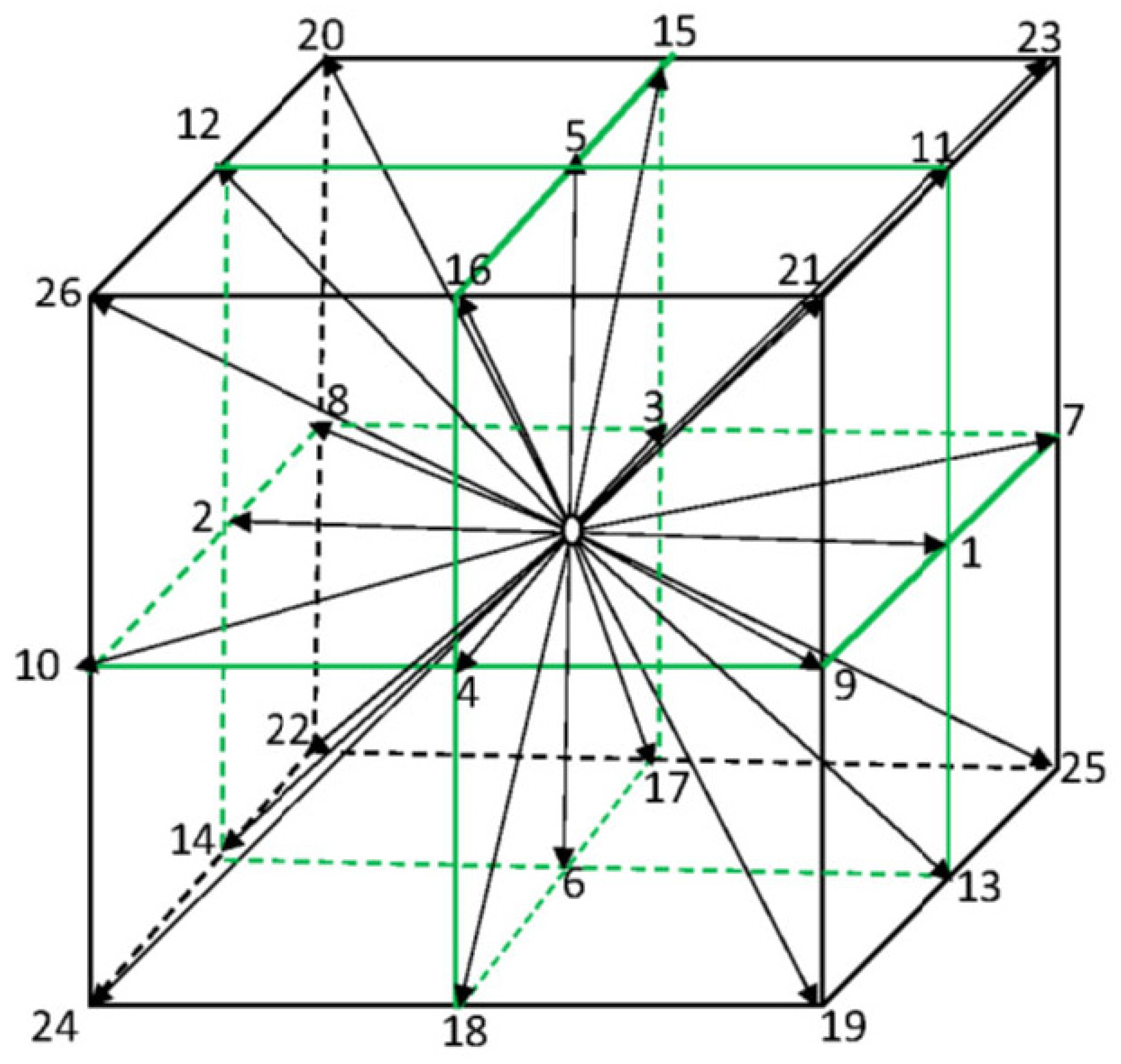
Figure 2.
Original HG functions with different asymetry coefficients (curves) and corresponging normalized HG functions (dots).
Figure 2.
Original HG functions with different asymetry coefficients (curves) and corresponging normalized HG functions (dots).
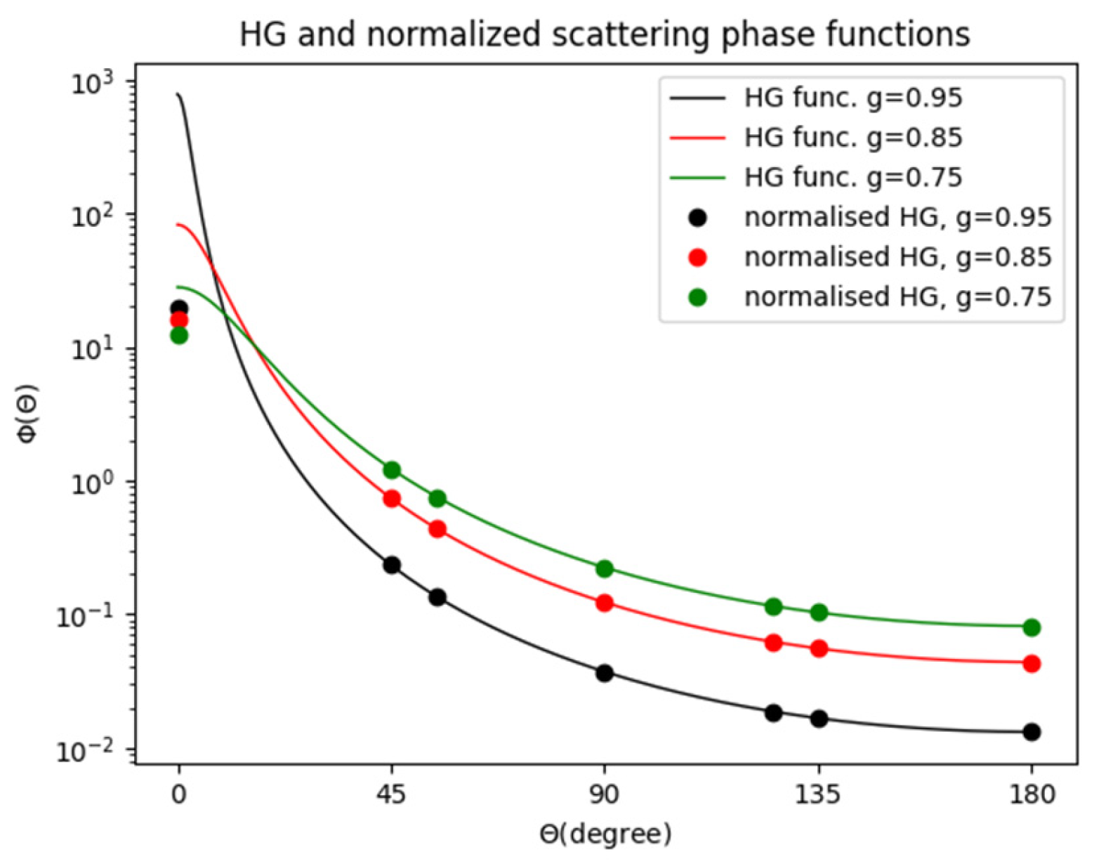
Figure 3.
Left panel: a sketch of the 3D computation domain, top beam income boundary and aerosol medium medium. Incoming top boundary is beam. Medium aerosol scattering albeo=1, optical depth=33.333, and scattering phase function parameter= 0.85. Right panel: a comparison of center vertical line samples (at xgrid=ygrid=51) of the RTLBM and RTMCM results.
Figure 3.
Left panel: a sketch of the 3D computation domain, top beam income boundary and aerosol medium medium. Incoming top boundary is beam. Medium aerosol scattering albeo=1, optical depth=33.333, and scattering phase function parameter= 0.85. Right panel: a comparison of center vertical line samples (at xgrid=ygrid=51) of the RTLBM and RTMCM results.
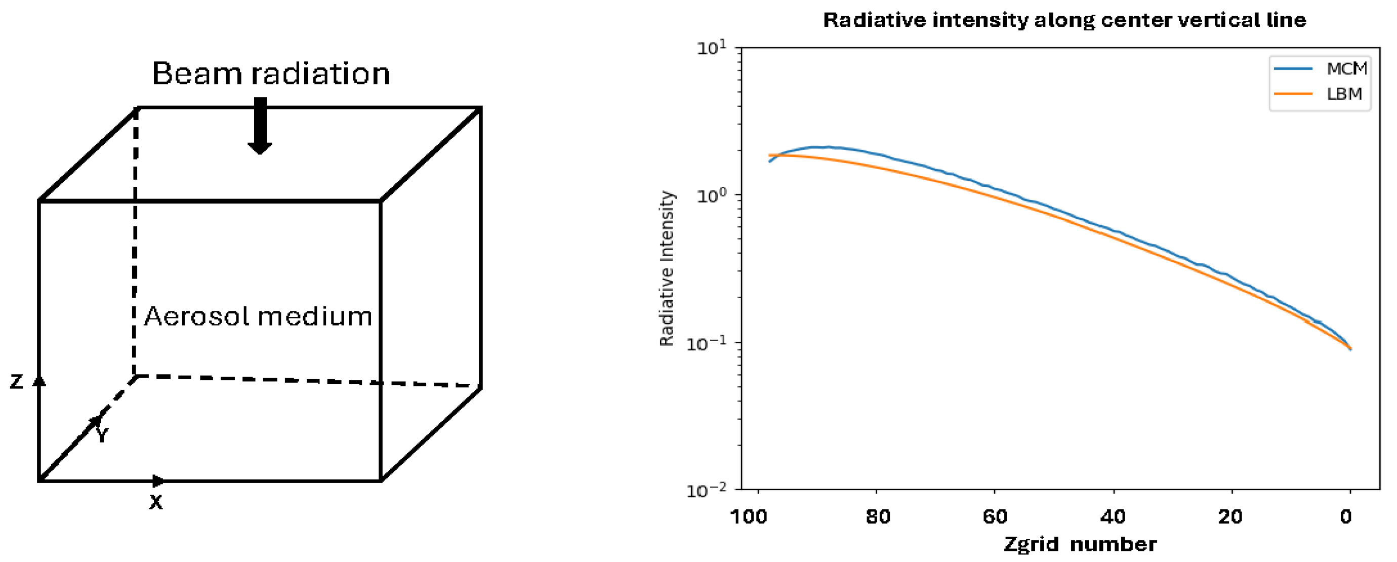
Figure 4.
A 3D display of vertical planes of RTLBM (left panel) and RTMCM (right panel) results. The numbers on the axises are grid numbers. Incoming top boundary is beam. Medium aerosol scattering albeo=1, optical depth=33.333, and scattering phase function parameter= 0.85.
Figure 4.
A 3D display of vertical planes of RTLBM (left panel) and RTMCM (right panel) results. The numbers on the axises are grid numbers. Incoming top boundary is beam. Medium aerosol scattering albeo=1, optical depth=33.333, and scattering phase function parameter= 0.85.
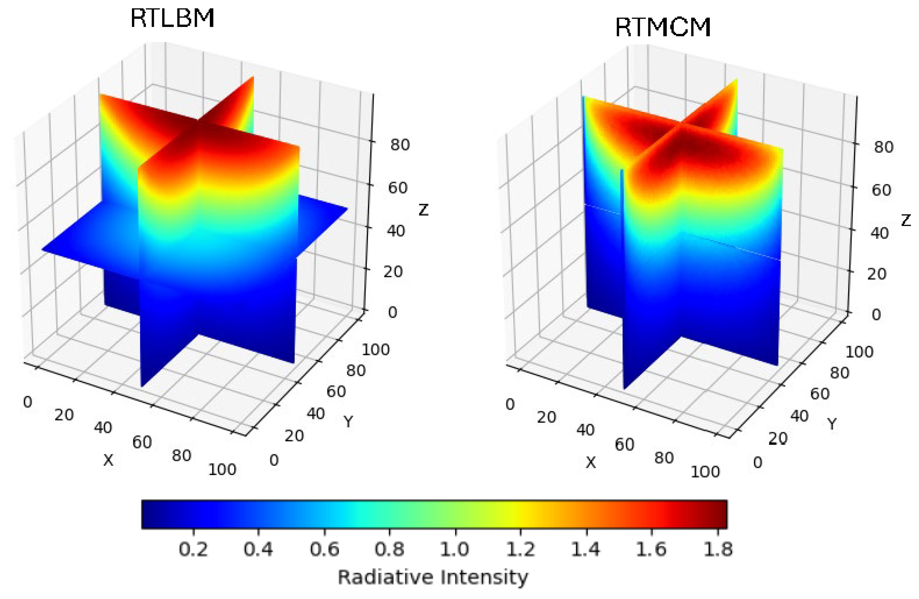
Figure 7.
Left panel: a sketch of the 3D computation domain, top beam income boundary radiation and mixed clear atmosphere cloud aerosol media. Clean air Rayleigh scattering optical depth= 0.08, scattering albedo=0.7. Cloud region albeo=1, optical depth=20, and scattering phase function parameter= 0.85; Right panel: a comparison of center vertical line samples (at X=Y=0.5) of the RTLBM and RTMCM.
Figure 7.
Left panel: a sketch of the 3D computation domain, top beam income boundary radiation and mixed clear atmosphere cloud aerosol media. Clean air Rayleigh scattering optical depth= 0.08, scattering albedo=0.7. Cloud region albeo=1, optical depth=20, and scattering phase function parameter= 0.85; Right panel: a comparison of center vertical line samples (at X=Y=0.5) of the RTLBM and RTMCM.
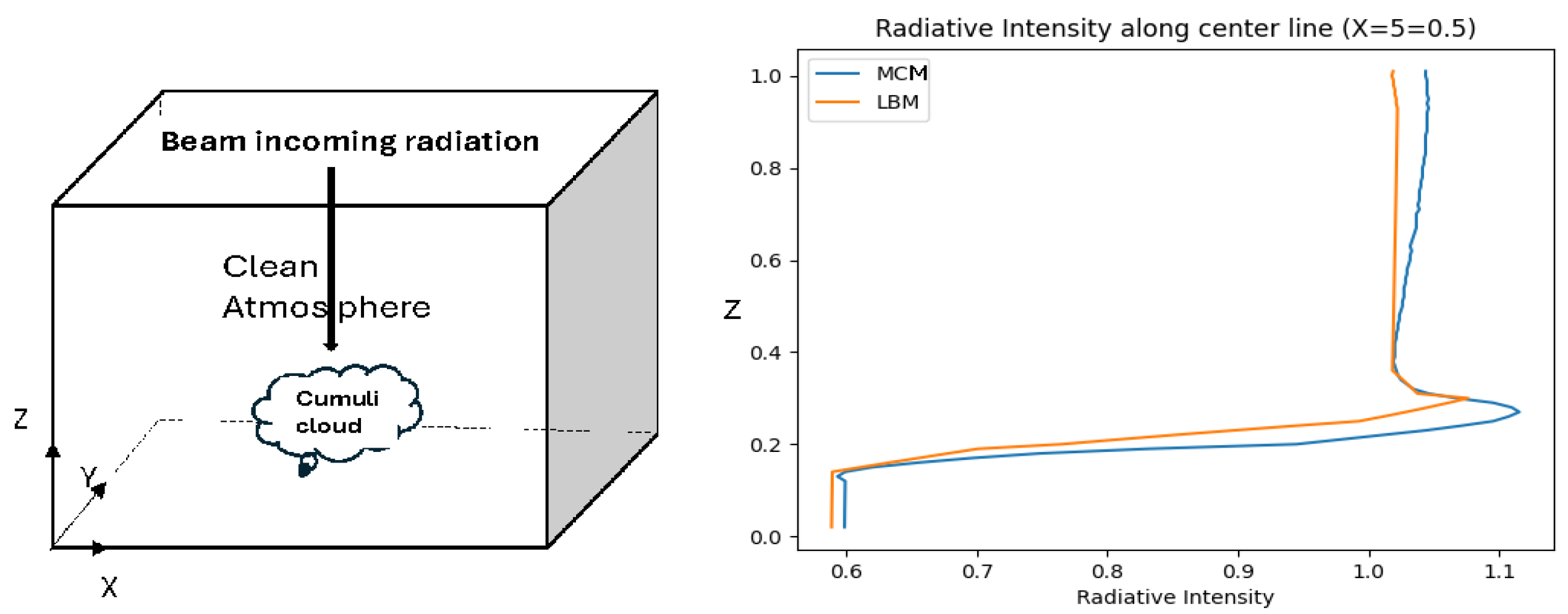
Figure 8.
A side by side comparison of RTLBM (left panel) and RTMCM (right panel) results for mixed clear atmosphere and cloud areosol media at the center plane cuts (Y=0.5) in the radiative filed.
Figure 8.
A side by side comparison of RTLBM (left panel) and RTMCM (right panel) results for mixed clear atmosphere and cloud areosol media at the center plane cuts (Y=0.5) in the radiative filed.
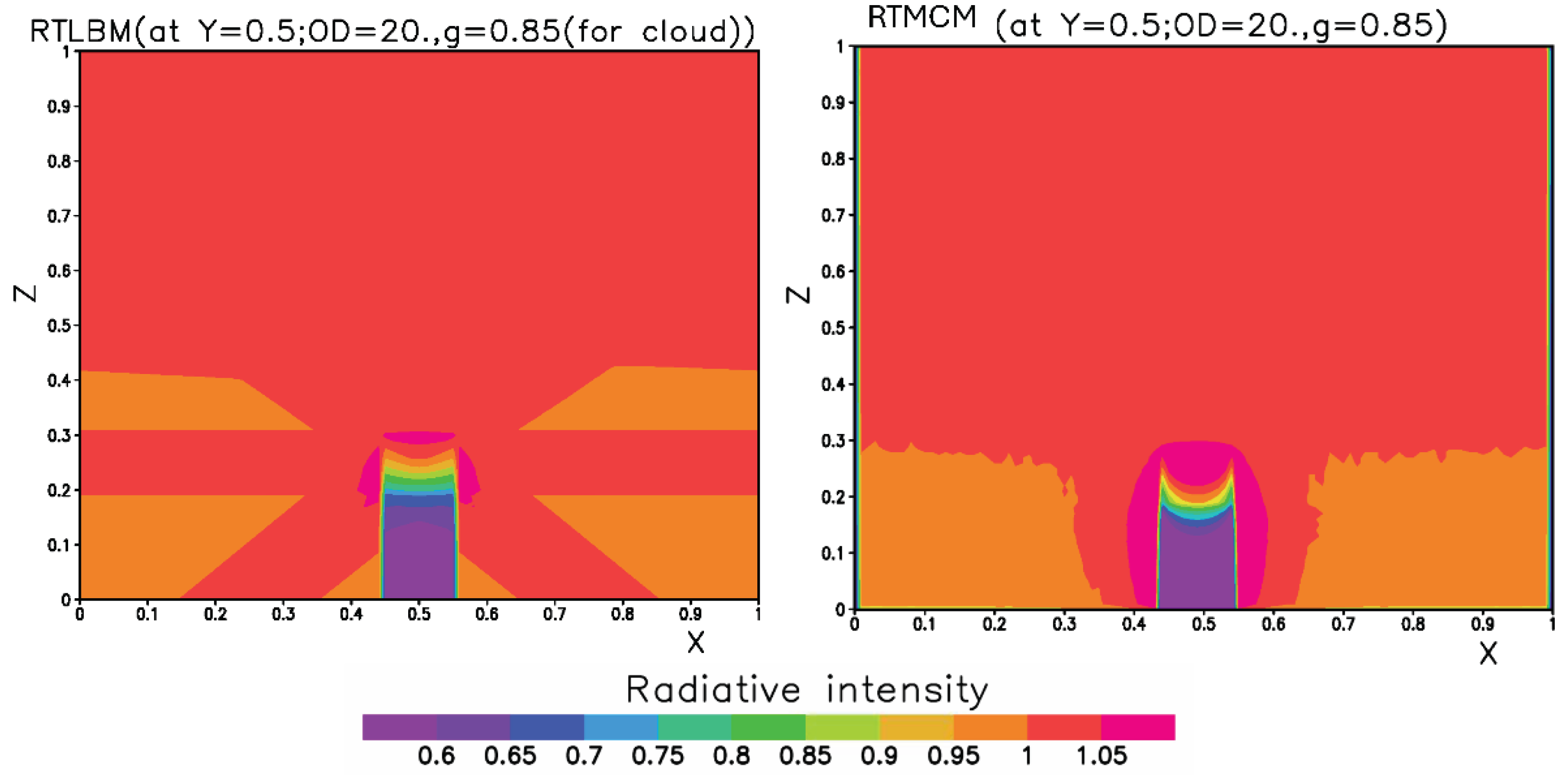

Table 1.
Computation time comparison of RTMCM and RTLBM using an Intel Xeon W-1200 CPU.
| Domain size RTMCM CPU time (sec.) |
RTLBM CPU time (sec.) |
RTMCM/RTLBM Time ratio |
|---|---|---|
| 101*101*101 18000 | 37 | 486 |
Table 2.
Computation time of RTLBM, Cuda kernel with C++ implementation.
| Domain size AMD 7713 CPU (sec.) |
Tesla A100 GPU (sec.) |
CPU/GPU Time ratio |
|---|---|---|
| 501*501*301 5835 | 32 | 182 |
| 501*501*501 15194 | 58 | 261 |
| 101*101*101 32.72 | 0.95 | 34 |
Table 3.
Computation time of RTLBM, Cuda kernel with Python implementation.
| Domain size AMD 7713 CPU (sec.) |
Tesla A100 GPU time (sec.) |
CPU/GPU Time ratio |
|---|---|---|
| 501*501*301 5835 | 38 | 154 |
| 501*501*501 15194 | 59 | 258 |
Disclaimer/Publisher’s Note: The statements, opinions and data contained in all publications are solely those of the individual author(s) and contributor(s) and not of MDPI and/or the editor(s). MDPI and/or the editor(s) disclaim responsibility for any injury to people or property resulting from any ideas, methods, instructions or products referred to in the content. |
© 2026 by the authors. Licensee MDPI, Basel, Switzerland. This article is an open access article distributed under the terms and conditions of the Creative Commons Attribution (CC BY) license (http://creativecommons.org/licenses/by/4.0/).
Copyright: This open access article is published under a Creative Commons CC BY 4.0 license, which permit the free download, distribution, and reuse, provided that the author and preprint are cited in any reuse.


