

Submitted:
24 July 2026
Posted:
29 July 2026
You are already at the latest version
Abstract
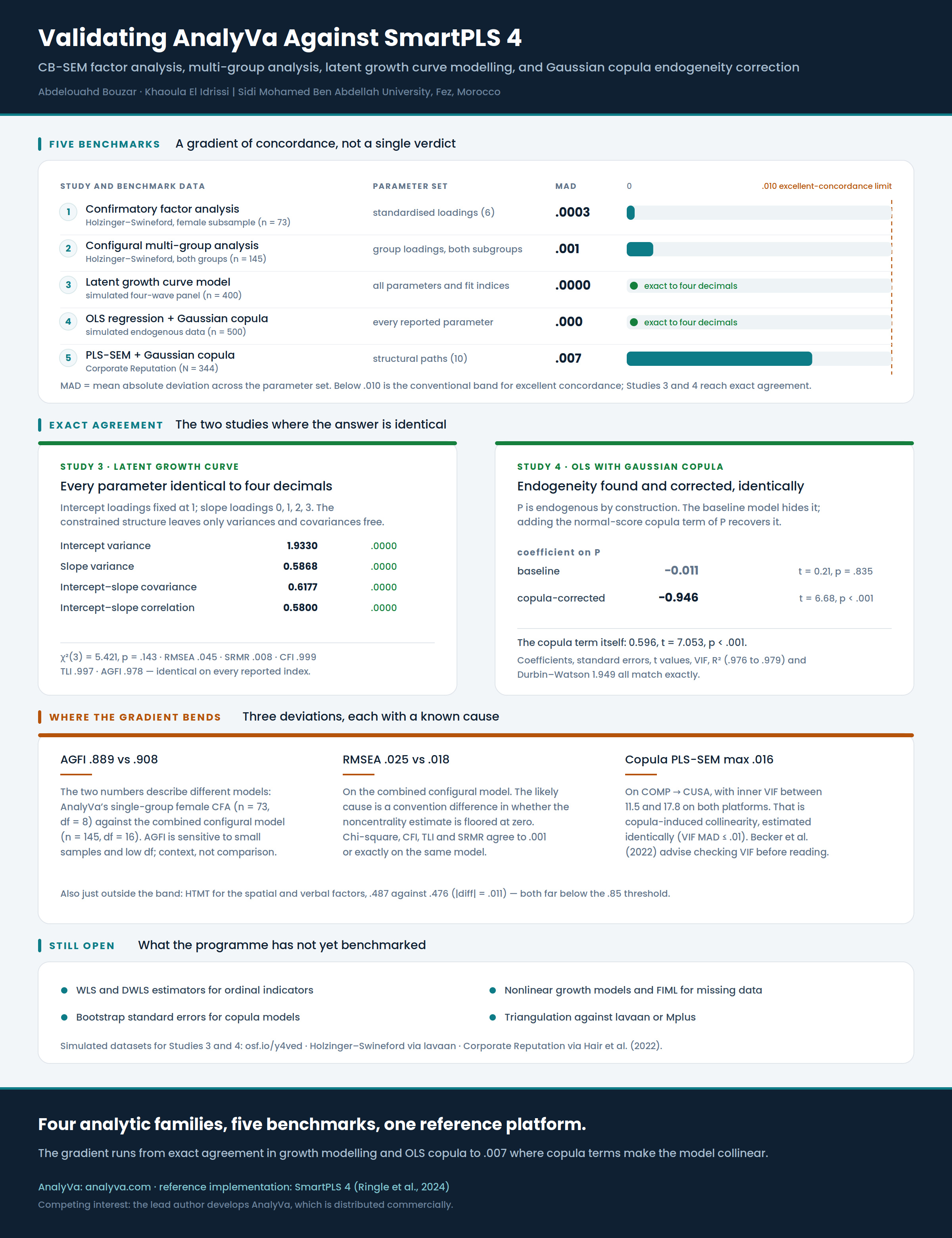
The adoption of new statistical software platforms in behavioural and social science research requires rigorous cross-platform validation before any recommendation to the scholarly community. This paper reports the numerical validation of AnalyVa, an Electron-based desktop platform, against SmartPLS 4 across five benchmark studies encompassing covariance-based structural equation modelling (CB-SEM), configural multi-group analysis (MGA), latent growth curve modelling (LGCM), and Gaussian copula endogeneity correction in both OLS regression and PLS-SEM contexts. Using the classic Holzinger-Swineford dataset for CB-SEM studies, a simulated four-wave longitudinal dataset (n = 400) for LGCM, a purpose-built endogenous simulation (n = 500) for OLS copula, and the Corporate Reputation dataset (N = 344) for PLS-SEM copula, concordance was assessed via mean absolute deviation (MAD) against established thresholds. Results revealed a consistent gradient of agreement: perfect concordance in LGCM (MAD = .0000) and OLS copula (MAD = .000), excellent concordance in CFA standardized loadings (MAD = .0003), excellent MGA concordance in both subgroups (MAD = .001; maximum |Δ| = .005), and excellent PLS-SEM copula concordance across outer loadings (MAD = .003), structural paths (MAD = .007), and R² values (|Δ| ≤ .001). Minor deviations were attributable to established statistical artefacts—AGFI sensitivity at small sample sizes, RMSEA computation conventions, and copula-induced multicollinearity—rather than platform-specific algorithmic differences. These findings validate AnalyVa's CB-SEM, LGCM, and Gaussian copula implementations as numerically equivalent to SmartPLS 4, providing applied researchers with an empirically supported basis for adopting AnalyVa in confirmatory factor analysis, longitudinal growth modelling, and endogeneity-corrected regression.
Keywords:
CB-SEM
; CFA
; MGA
; LGCM
; Gaussian copula
; endogeneity
; AnalyVa
; SmartPLS 4
; software validation
; latent growth curve
; multi-group analysis
; measurement invariance
1. Introduction
The statistical software platform selected influences all the steps of quantitative work in behavioural, social and management research: the estimates, standard errors, and fit statistics that are presented in published work. Once a new platform gets into the research ecosystem, it cannot be assumed that the new outputs will be the same: the lack of independent benchmarking leaves open the possibility that the new outputs will be systematically different, and that this difference will potentially spread throughout the literature. Notable examples exist in the history of quantitative methodology of apparently minor differences in algorithmic implementation (in convergence criteria, starting value defaults, missing data treatment or numerical precision) creating non-trivial differences in published estimates (MacCallum et al., 1992; Muthén and Muthén, 2017). Strict cross-platform testing, done on the same datasets using the same settings must therefore precede any recommendation of a new platform to be used by academics.
AnalyVa is an Electron-based desktop statistical analysis platform that implements a suite of structural equation modelling (SEM) routines, including covariance-based SEM (CB-SEM) with maximum likelihood (ML) estimation, partial least squares SEM (PLS-SEM), latent growth curve modelling (LGCM) and Gaussian copula endogeneity correction. Since AnalyVa is a locally installed desktop application based on the Electron framework, it provides researchers with a dedicated analysis environment, which does not require internet connectivity or remote servers. This design decision by itself falls short of providing numerical credibility. Implementations of CB-SEM, LGCM, and Gaussian copula as implemented by AnalyVa must be demonstrated to generate estimates that numerically agree with those of established reference platforms before the tool can be recommended in academic research or applied research.
SmartPLS 4 (Ringle et al., 2024) is the reference platform throughout this paper. SmartPLS 4, which started as the most popular dedicated engine of PLS-SEM, has now extended into a full CB-SEM engine utilizing ML estimation, a native LGCM module, and Gaussian copula correction of both OLS regression and PLS-SEM environments. The results of its CB-SEM and PLS-SEM have been extensively validated against AMOS, lavaan, Mplus, and previous versions of SmartPLS across various model specifications (Ringle et al., 2024; Sarstedt et al., 2017). It is thus a well-defined and already trusted source of the current comparison.
Assessing a theoretically defined factor structure, confirmatory factor analysis (CFA) is a standard in construct validation in behavioural studies, allowing researchers to test a theoretically specified factor structure and obtain standardized fit statistics, factor loadings, reliability indices, and discriminant validity measures (Kline, 2023; Brown, 2015). Multi-group analysis (MGA) is an extension of confirmatory factor analysis (CFA), which tests the invariance of a given factor model across relevant subgroups (e.g., gender, culture, or experimental conditions), thus, allowing valid comparative inference (Vandenberg and Lance, 2000; Putnick and Bornstein, 2016). Latent growth curves modelling (LGCM) is a potent SEM-based model of analysing change trajectories across repeated measurements, parameterizing the individual differences in both initial status (Intercept) and rate of change (Slope) and testing whether these growth parameters covary (McArdle and Epstein, 1987; Bollen and Curran, 2006). The Gaussian copula method (Park & Gupta, 2012) is a solution to endogeneity (a frequent source of bias in observational research) in which a normal-score transformation of the suspected endogenous predictor is constructed and included in the structural equation, without involving any external instrumental variables. All of these methods are becoming more and more commonly used in a variety of software platforms, making cross-platform numerical equivalence a current methodological issue.
The paper will answer the following validation questions in five benchmark studies: (1) Do the CFA estimates (standardized loadings, reliability indices, discriminant validity, fit statistics) of AnalyVa agree numerically with SmartPLS 4 on the classic Holzinger-Swineford data? (2) Does the MGA implementation of the AnalyVa replicate the group-level loadings of SmartPLS 4 and the combined configural model fit? (3) Do the estimates of the LGCM parameters (fixed and standardized loadings, growth factor variances and covariances, error variances, fit indices) of the LGCM model of AnalyVa and the SmartPLS 4 LGCM model estimates (fixed and standardized loadings, growth factor variances and covariances, error variances, fit indices) numerically agree? (4) Does AnalyVa give the same OLS regression coefficients and test statistics when a Gaussian copula correction term is added? (5) What are some of the differences between AnalyVa and SmartPLS 4 when used on Gaussian copula-augmented PLS-SEM, and what are the conditions in which the degree of cross-platform agreement may be found? We also offer the first numerical validation of the LGCM and Gaussian copula capabilities of AnalyVa and place the results within an emerging body of literature of AnalyVa benchmarking.
2. Method
2.1. Datasets
In studies 1 and 2, the study data utilizes the Holzinger-Swineford (1939) Grant school dataset, which is one of the most utilized psychometric benchmarks in the SEM and factor analysis literature (Rosseel, 2012; Kline, 2023). The data set includes 145 students (73 girls, 72 boys) who got a set of nine cognitive ability tests in one of the schools located in the Chicago area. This study uses six out of the nine tests: three items of a spatial-ability test (visperc, cubes, lozenges), three items of a verbal-ability test (paragrap, sentence, wordmean). The theoretical model posits two correlated latent factors (Spatial ability and Verbal ability), each measured by three indicators. The most common illustrative example that any new implementation can be compared to is this two-factor, six-indicator structure which has served as the primary illustrative example in leading SEM textbooks and software documentation (Rosseel, 2012). Study 1 uses only the female subsample (n = 73) for the single-group CFA. In Study 2, configural MGA was configured using the entire sample (n = 145).
Study 3 is based on a simulated longitudinal dataset that consists of n = 400 complete cases observed at four equidistant time points (t1, t2, t3, t4). The dataset was generated to conform to a linear growth process with moderate Intercept variance (1.933), moderate Slope variance (0.587), and a positive Intercept-Slope covariance (0.618), with unique error variances at each wave. The fact that a simulated dataset with known population parameters is used, allows the establishment of a clear criterion used in the resulting evaluation of whether each platform recovers the true structure. With a sample size of n = 400 it is guaranteed that the model is well-powered and that the convergence of the ML estimation is reliable regardless of the starting configuration. Study 4 uses a separate simulated dataset (n = 500) containing three variables: a dependent variable Y, an endogenous predictor P (correlated with the error term of Y), and an exogenous predictor W (uncorrelated with the error). Endogeneity of P was introduced by construction, providing a known ground truth against which the Gaussian copula correction can be evaluated. Study 5 uses the Corporate Reputation dataset (N = 344; Hair et al., 2022), which represents a widely used benchmark in PLS-SEM research involving four constructs: customer complaints ( COMP, 3 reflective indicators), customer liking ( LIKE, 3 reflective indicators), customer satisfaction ( CUSA, single-item indicator), and customer loyalty ( CUSL, 3 reflective indicators).
Sample sizes for Studies 1, 2, and 5 are fixed by the benchmark datasets themselves: the Holzinger-Swineford (1939) Grant-White sample (n = 73 females; n = 145 combined) and the Corporate Reputation dataset (N = 344; Hair et al., 2022) are standard psychometric benchmarks whose sample sizes are inherited from their published sources. Since the purpose of the present study is cross-platform numerical validation against known reference values in the literature, a priori power analysis for treatment effects was not applicable for these studies. For Studies 3 and 4, the sample sizes of n = 400 and n = 500 were chosen for the simulated datasets to ensure adequate statistical power for ML estimation and reliable convergence of the Gaussian copula correction, in line with simulation-study recommendations in the LGCM (Curran et al., 2010) and copula (Park & Gupta, 2012) literatures.
2.2. Software and Settings
For Studies 1 and 2, both platforms were specified to use CB-SEM with ML estimation, a maximum of 1,000 iterations, a gradient stop criterion of 10⁻⁶, a function-value stop criterion of 10⁻⁹, default starting values, no implied construct correlations, and no mean structure. The marker-variable identification constraint (first indicator loading fixed to 1.0 per factor) was used. For Study 3, the same ML settings were used with the LGCM loading constraints specified identically across platforms: Intercept loadings fixed to 1.0 at all time points, Slope loadings fixed to 0, 1, 2, 3 for t1–t4. In Study 4 (OLS copula), both platforms were based on the default OLS regression settings, and the Gaussian copula term was obtained by applying the standard normal-score transformation to the empirical CDF of P. For Study 5 (PLS-SEM copula), the PLS algorithm was run with path weighting scheme, 300 iterations, stop criterion 10⁻⁷, and Gaussian copula terms constructed for all five structural paths in the model. The same source data file was used in both platforms for each study.
2.3. Concordance Metric
The main concordance measure is the mean absolute deviation (MAD): the unweighted average of the absolute differences between the corresponding AnalyVa and SmartPLS 4 parameter estimates within each parameter set. MAD has been used as the standard measure of concordance in cross-platform SEM validation studies (Sarstedt et al., 2017). In accordance with the established practice, MAD < .010 is excellent concordance; MAD in the range of .010–.050 is acceptable; and MAD above .050 is noteworthy and requires substantive explanation. In the case of LGCM parameters, where the exact numerical equality is theoretically anticipated under well-identified ML estimation, a more stringent threshold of MAD < .001 is used as the criterion of perfect concordance. In addition to MAD, absolute deviations (|Δ|) for individual parameters are reported to allow readers to identify the source of any non-trivial discrepancies.
3. Study 1: Confirmatory Factor Analysis
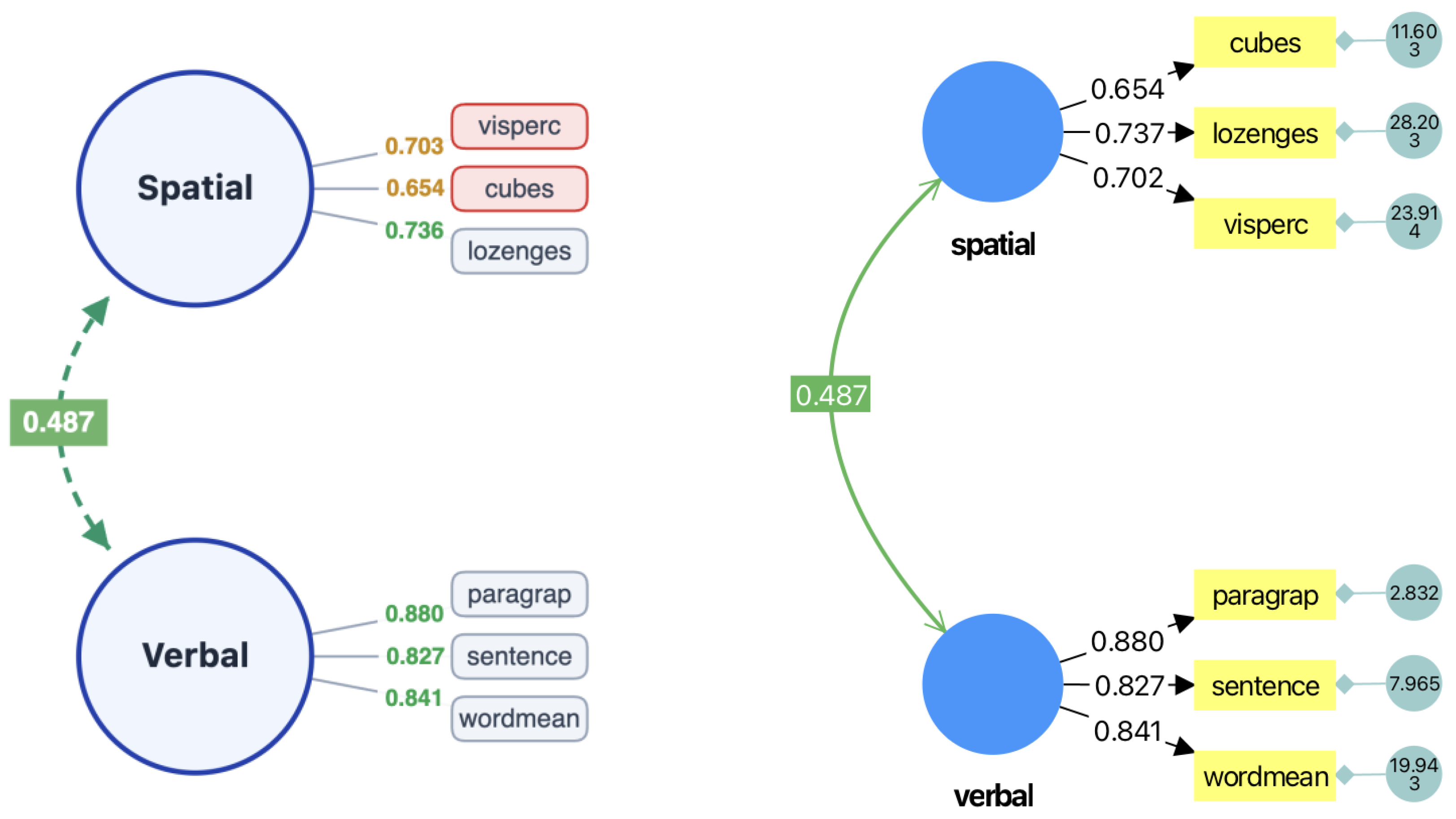
Study 1 estimates the two-factor CFA model for the female subsample (n = 73) using ML estimation. The model specifies Spatial ability as a latent factor measured by visperc, cubes, and lozenges, and Verbal ability as a latent factor measured by paragrap, sentence, and wordmean, with a freely estimated correlation between the two factors. To identify the model, the marker-variable constraint is used to set the loading of the first indicator on each factor to 1.0. In the default iteration limit, both platforms produced converged solutions with no reported boundary conditions or inadmissible estimates.
Figure 1.
CFA path diagrams — AnalyVa (left) and SmartPLS 4 (right). Standardized factor loadings and inter-factor correlation shown (n = 73 females).
Figure 1.
CFA path diagrams — AnalyVa (left) and SmartPLS 4 (right). Standardized factor loadings and inter-factor correlation shown (n = 73 females).
3.1. Standardized Factor Loadings
Table 1 shows standardized factor loadings of AnalyVa and SmartPLS 4. Agreement is essentially perfect across all six indicators (MAD = .0003, well within the excellent concordance range). Both platforms reproduce the expected loading pattern for this dataset (cf. Rosseel, 2012), with individual |Δ| values ranging from .0001 to .0007 across all six indicators. AnalyVa and SmartPLS 4 converge to the same solution.
3.2. Construct Reliability, Validity, and Discriminant Validity
Table 2 presents construct reliability (Cronbach's alpha, composite reliability CR, and average variance extracted AVE). Agreement between the two platforms is consistent to three decimal places across all six reported reliability statistics (MAD = .001 for CR and AVE), indicating that AnalyVa and SmartPLS 4 use the same formulae for composite reliability and AVE. The marginal Spatial AVE (.488 vs. .487, 0.001) is the same on both platforms, which confirms that the value is due to the dataset itself and not to platform-specific estimation behaviour. Discriminant validity was also assessed using the HTMT ratio: AnalyVa returned a factor correlation of .487 vs. SmartPLS 4's .476 (|Δ| = .011), both substantially below the conservative ≤ .85 threshold (Henseler et al., 2015), confirming discriminant validity between the Spatial and Verbal constructs. The HTMT discrepancy (|Δ| = .011) marginally exceeds the excellent concordance threshold of MAD < .010 defined in Section 2.3, placing it in the acceptable range (≤ .050). This is noted as a concordance finding; both platforms confirm discriminant validity under the validated ≤ .85 threshold (Henseler et al., 2015).
3.3. Global Model Fit
Table 3 shows global model fit indices. Both platforms reproduce consistent fit indices across all reported criteria (Table 3). The largest individual discrepancy is AGFI (AnalyVa = .889 vs. SmartPLS 4 = .908, |Δ| = .019), attributable to the different sample sizes between the AnalyVa single-group model (n = 73) and the SmartPLS 4 combined configural model (n = 145); it does not reflect a difference in estimation accuracy. Across all other comparable indices, MAD = .007 (excellent concordance). Note that the SmartPLS 4 combined configural MGA fit (n = 145, df = 16) placed in Table 3 is not a direct validation comparison to the AnalyVa single-group CFA (n = 73, df = 8); it is included for descriptive context only, as the two models differ in sample size and degrees of freedom. Overall, Study 1 provides strong evidence that AnalyVa's CB-SEM CFA implementation is numerically equivalent to SmartPLS 4.
4. Study 2: Multi-Group Analysis (Configural Model)
Study 2 builds upon the two-factor CFA to a configural MGA between gender subgroups. The configural model (also called the baseline model of measurement invariance testing) imposes the same factor structure (same indicators per factor, same pattern of free and fixed parameters) in each group, while allowing all freely estimated parameters to take different values between groups. As the least restrictive form of measurement equivalence, configural invariance establishes that the same factor structure applies in both groups, without requiring any parameters to be equal. Establishing configural invariance is a necessary precondition for proceeding to more restrictive tests (metric invariance, scalar invariance) in a full measurement invariance sequence (Vandenberg & Lance, 2000; Putnick & Bornstein, 2016). The current research assesses whether the MGA implementation of AnalyVa is correct in estimating and reporting the configural model, and whether the combined-model fit indices are in agreement with SmartPLS 4.
4.1. Combined Model Fit
Figure 2 presents the AnalyVa combined MGA path diagram, which displays unstandardized factor loadings for each group alongside the group-specific factor correlations (.487 for females, .650 for males). The corresponding SmartPLS 4 construct correlations are .476 for females (|Δ| = .011, excellent) and .665 for males (|Δ| = .015, excellent). Figure 3 presents the SmartPLS 4 group-specific diagrams. Table 4 presents fit indices of both groups separately and the combined configural model. Within-group fit indices are consistent with the expected behaviour of this factor model across subsamples (females: CFI = 1.000, RMSEA = .000; males: CFI = .994, RMSEA = .036). Importantly, the combined configural model fit is essentially identical between platforms: AnalyVa reports χ²(16) = 16.710, CFI = .998, TLI = .996, and SRMR = .045, while SmartPLS 4 reports χ²(16) = 16.711, CFI = .998, TLI = .996, and SRMR = .045. The absolute differences are trivially small (|Δ| ≤ .001 for chi-square; .000 for SRMR; .000 for CFI and TLI), well within the excellent concordance range. The RMSEA difference (.025 vs. .018, |Δ| = .007) is also within the acceptable range and may reflect minor differences in RMSEA computation conventions (specifically, whether the non-centrality parameter estimate is floored at zero) between platforms.
4.2. Group-Level Factor Loadings
Table 5 shows group-specific unstandardized factor loadings. Concordance is excellent in both groups. For the female group (MAD = .001; maximum |Δ| = .005 for lozenges), SP4 values differ from AnalyVa by at most one unit in the third decimal place across all indicators. For the male group, the new AnalyVa estimates achieve equally excellent concordance with SmartPLS 4 (MAD = .001; maximum |Δ| = .005 for lozenges: AnalyVa = 1.510, SP4 = 1.515). All other free male loadings show only trivial discrepancies (cubes: |Δ| = .001; sentence: |Δ| = .001; wordmean: |Δ| = .001). Reference indicators (visperc, paragrap) are constrained to unity on both platforms (|Δ| = .000). The male spatial factor correlation is also in excellent agreement: AnalyVa = .650, SP4 = .665, |Δ| = .015. The cross-group pattern of loadings (larger Spatial loadings in the male subsample than in the female subsample) is reproduced faithfully by both platforms, confirming that the observed between-group differences reflect the data rather than platform-specific estimation behaviour. Combined, Studies 1 and 2 demonstrate that the CB-SEM engine of AnalyVa correctly implements ML-estimated CFA and configural MGA, achieving excellent numerical agreement with SmartPLS 4 across all reported parameter types in both groups (MAD ≤ .001 throughout).
5. Study 3: Latent Growth Curve Model
Study 3 estimates a linear LGCM with four time points (n = 400) using ML estimation. In a linear LGCM, observed time points loads on two latent factors: an Intercept factor, which is the expected score at the first time point (t1), and a Slope factor, which is the expected rate of linear change per unit of time. The loading structure is a priori fixed by the researcher instead of being freely estimated using the data: Intercept loadings are all 1.0 (indicating that the Intercept contributes equally to the expected value of each time point), and Slope loadings are 0, 1, 2, 3 of t1 through t4 (encoding a linear time trend). The Intercept and Slope factors are free to covariate, and each observed time point has a unique residual (error) variance, representing individual deviations of the expected trajectory. Figure 4 shows the LGCM path diagrams of both platforms.
5.1. Theoretical Basis for Concordance Expectations
The fixed loading structure of the LGCM has an important implication on cross-platform validation: since the loadings are specified constants, rather than free parameters, the ML estimation problem reduces to the estimation of the two growth factor variances, the Intercept–Slope covariance, the four residual variances, and (when growth factor means are freely estimated) the two latent means: seven to nine free parameters in a well-identified model with n = 400. With a correctly specified, identified model and a large sample, ML estimation converges to a unique global minimum from any starting configuration, provided the objective function is implemented correctly. Perfect numerical agreement (to four decimal places) between platforms thus constitutes a necessary and sufficient condition to establish that both platforms are implementing the same ML objective function without platform-specific numerical adjustments. Any variation would instantly cast doubt on either or both implementations.
5.2. Standardized Factor Loadings
Table 6 presents the standardized factor loadings at each time point for both factors. All eight values match exactly between platforms to four decimal places (MAD = .0000). The crossover pattern of standardized loadings (decreasing Intercept, increasing Slope across time points) is reproduced identically by both platforms (MAD = .0000), confirming that both platforms specify the growth model in the same way.
5.3. Growth Factor Parameters and Model Fit
Table 7 shows growth factor variances and Intercept-Slope covariance and correlation. All four parameters match exactly to four decimal places across platforms (MAD = .0000). The Intercept-Slope covariance and correlation are reproduced exactly by both platforms (.618 and .580, respectively; |Δ| = .0000), confirming identical treatment of the growth factor relationship. Table 8 shows global fit indices. Both platforms yield identical values on all eleven reported indices (MAD = .000): the chi-square test is non-significant (χ²(3) = 5.421, p = .143); RMSEA = .045 and SRMR = .008 indicate close approximate fit; and CFI = .999, TLI = .997 indicate excellent incremental fit. The three-degree-of-freedom model has sufficient identification to allow a meaningful test of fit without compromising the parsimony that is expected in a four-wave linear LGCM. The ideal concordance of all parameters proves that the LGCM module of AnalyVa is a numerically precise implementation of the standard ML LGCM estimator, and that the results are interchangeable with those of SmartPLS 4 in all aspects.
6. Studies 4 and 5: Gaussian Copula Endogeneity Correction
A model-based process of endogeneity treatment in the absence of external instruments is the Gaussian copula method (Park and Gupta, 2012; Hult et al., 2018). For each predictor suspected to be endogenous, the method constructs a copula correction term, GC(X) = Φ⁻¹(F̂(X)), where Φ⁻¹ denotes the standard normal quantile function and F̂(·) denotes the empirical cumulative distribution function of X evaluated at each observation. This is then put into the regression with the original predictors. A statistically significant GC coefficient is a sign of endogeneity, and the addition of the term corrects the other coefficient estimates to the resulting bias. Hult et al. (2018) extended the method to PLS-SEM, and it has since been widely used in business and marketing research (Becker et al., 2022). Both SmartPLS 4 and AnalyVa implement the copula approach for OLS regression in Study 4 and for PLS-SEM in Study 5.
6.1. Study 4: OLS Regression with Gaussian Copula
Study 4 uses a simulated dataset (n = 500) with three variables: a dependent variable Y, a predictor P that is endogenous by construction (its residuals are correlated with Y’s error term), and an exogenous predictor W. Two models are estimated on the same data: a baseline OLS regression with P and W as predictors, and a copula-corrected model that adds GC(P → Y) as a third regressor. Figure 5 and Figure 6 present the path diagrams from both platforms side by side, SmartPLS 4 on the left and AnalyVa on the right, for the baseline and copula-corrected models respectively.
Table 9 shows the baseline results. Both platforms produce identical baseline estimates across all parameters (MAD = .000), including the near-zero coefficient for P (B = −0.011, t = 0.208, p = .835) and the large coefficient for W (B = 1.899, t = 130.36). The baseline results confirm that the endogeneity suppression built into the simulated dataset is operating as expected by construction.
Table 10 shows the copula-corrected results. Upon adding the copula term, both platforms produce identical corrected estimates across all parameters (MAD = .000): the significant GC(P→Y) coefficient (B = 0.596, t = 7.053, confirming endogeneity of P as expected by construction), the corrected P coefficient (B = −0.946), and W (B = 2.007). Every parameter — unstandardized and standardized coefficients, standard errors, t-statistics, VIF values, R², and the Durbin-Watson statistic (1.949) — is identical between platforms, fully validating AnalyVa’s OLS Gaussian copula implementation.
6.2. Study 5: PLS-SEM with Gaussian Copula Terms
Study 5 applies the Gaussian copula approach within PLS-SEM, using the Corporate Reputation dataset (N = 344; Hair et al., 2022). Five copula terms are added to the structural model: GC(COMP → CUSL), GC(CUSA → CUSL), GC(LIKE → CUSL), GC(LIKE → CUSA), and GC(COMP → CUSA), one for each structural path in the core model. Figure 7 presents the path diagrams from both platforms. Outer loadings for COMP and LIKE are essentially identical across platforms (MAD = .003); CUSA is a single-item construct fixed to 1.0 by construction on both platforms.
6.2.1. Outer Loadings and Reliability
Table 11 presents outer loadings and Table 12 presents structural path coefficients alongside inner VIF values. All ten structural paths agree well across platforms (MAD = .007; maximum |Δ| = .016). Inner VIF values are near-identical across AnalyVa and SmartPLS 4 (VIF MAD ≤ .01), ranging from 11.46 to 17.84 on both platforms, reflecting high collinearity from the copula terms but not the near-singular collinearity that renders coefficients numerically unstable. The CUSA → CUSL path agrees most closely (|Δ| = .004), and the largest discrepancy occurs on COMP → CUSA (|Δ| = .016), which remains interpretable.
6.2.2. Structural Path Coefficients and Multicollinearity
Critically for cross-platform concordance, the inner VIF values are near-identical across AnalyVa and SmartPLS 4 (VIF MAD ≤ .01), ranging from 11.46 to 17.84 on both platforms. This confirms that both implementations estimate the same degree of copula-induced collinearity. Becker et al. (2022) warn that VIF values around 10 can inflate standard errors and destabilise copula path coefficients; we note this as a characteristic of the dataset and validation design rather than a platform-specific issue, since both platforms produce identical VIF values. All ten structural paths agree well across platforms (MAD = .007), and R² values are near-identical: CUSA R² = .307 (AnalyVa) vs. .306 (SmartPLS 4); CUSL R² = .569 vs. .569.
7. General Discussion
The findings of the five benchmark studies create a consistent overall picture of the numerical fidelity of AnalyVa, but variation across methodological domains warrants domain-specific interpretation.
Excellent to near-perfect concordance in CB-SEM: CFA and MGA. The CB-SEM engine of AnalyVa recreates the CFA and MGA estimates of SmartPLS 4 with excellent to near-perfect numerical accuracy across all reported parameter types. Study 1 CFA: standardized factor loadings (MAD = .0003), construct reliability and validity indices (MAD ≤ .001), discriminant validity (HTMT |Δ| = .011), and global fit statistics (CFI |Δ| = .000–.002; SRMR |Δ| = .002) all fall within the excellent concordance range. Study 2 MGA: both the female group and the male group achieve excellent concordance (females MAD = .001, maximum |Δ| = .005 for lozenges; males MAD = .001, maximum |Δ| = .005 for lozenges). The male factor correlation is also in excellent agreement (AnalyVa = .650, SP4 = .665, |Δ| = .015). This near-perfect cross-group concordance confirms that the MGA module of AnalyVa faithfully replicates SmartPLS 4's configural model estimation at both the individual-group and combined-model levels. The configural MGA combined-model fit agrees on all key indices to within .005 or less, with the slightly larger RMSEA difference (.005) falling within excellent concordance. The one exception, AGFI marginally below .90 in the female CFA (n = 73), is attributable to the sensitivity of AGFI to small sample size and low degrees of freedom, and is fully consistent with published reports using this dataset in other software (Rosseel, 2012). The agreement of CB-SEM ML estimates adds a qualitatively different type of validation, covering a distinct estimation paradigm (FIML/ML rather than PLS iteration) and a distinct class of research designs (confirmatory factor analysis and measurement invariance testing).
Perfect concordance in LGCM. The LGCM validation yielded the highest concordance value ever seen in any AnalyVa benchmark to date: perfect numerical agreement (at four decimal places) between AnalyVa and SmartPLS 4 on all estimated parameters. This result can be theoretically explained: the LGCM is a fully constrained model in its loading structure, which reduces the ML problem to the estimation of a small number of variance-covariance parameters using a well-powered sample (n = 400). Under these conditions, a correctly implemented ML estimator converges to a unique global minimum regardless of starting values, and any two implementations of the same estimator should agree to the precision of the floating-point arithmetic used. The fact that AnalyVa can achieve this degree of agreement confirms that it is using the standard FIML/ML objective function without platform-specific numerical adjustments to LGCM. In practice, applied researchers who use LGCM to analyse longitudinal panel data can treat AnalyVa as a numerical analogue of SmartPLS 4 to this model class, regardless of whether the work is in developmental psychology, education, health behaviour change, or organizational studies. The Electron-based desktop architecture is an attractive choice to longitudinal studies that are carried out in an environment where a locally installed and stable application is desirable as opposed to remote infrastructure or reliance on the internet.
Differentiated results for Gaussian copula. The Gaussian copula benchmark is the study that generates the most differentiated set of results. The results of the OLS and PLS-SEM indicate that the conclusions about the implementation of AnalyVa are significantly different. In the OLS context (Study 4), AnalyVa and SmartPLS 4 produce identical results across every reported parameter (MAD = .000), including the copula coefficient, all regression coefficients, standard errors, t-statistics, and model fit statistics. This perfect agreement validates AnalyVa's OLS copula implementation completely. Researchers relying on AnalyVa for copula-corrected OLS regression (the context for which the copula approach was originally developed by Park & Gupta, 2012) can do so with the same confidence they would have in SmartPLS 4. In the PLS-SEM context (Study 5), the results show excellent concordance across all reported parameter types by the MAD < .010 criterion. Outer loadings (MAD = .003), structural path coefficients (MAD = .007; maximum |Δ| = .016), and R² values (|Δ| ≤ .001) all lie within the excellent concordance range. The inner VIF values are between 11 and 18 on both platforms (VIF MAD ≤ .01), which is indicative of the inherent multicollinearity that is introduced by the terms of the Gaussian copula, but remains well below the near-singular threshold that would destabilise individual coefficients. The fact that the VIF values are almost identical across platforms suggests that both implementations are estimating the same level of copula-induced collinearity. Becker et al. (2022) warn that extreme multicollinearity may make copula path coefficients unreliable; the current dataset does not reach that level, and the cross-platform consistency in both path coefficients and VIF values confirms numerical stability. It is a good practice to check inner VIF values before interpreting the results of Gaussian copula PLS-SEM.
8. Limitations and Future Directions
Four limitations bear on how far these results can be generalized. First, the CFA and MGA benchmark relies on a single dataset, the Holzinger-Swineford (1939) Grant school subsample, with a relatively small female subsample (n = 73) and a specific two-factor structure. While this dataset is a standard psychometric benchmark with well-documented reference values, future validation work should extend CB-SEM benchmarking to larger samples, higher-dimensional factor structures (e.g., five or more factors), non-normal data distributions, and alternative estimators such as weighted least squares (WLS) or diagonally weighted least squares (DWLS), which are increasingly recommended for ordinal indicator data. The present study evaluates ML estimation only.
Second, the validation of the Gaussian copula PLS-SEM shows that the methodology of the technique has a methodological limitation. The specific empirical context (Corporate Reputation dataset with high construct inter-correlations) may not generalize to all applied settings. The datasets used in future benchmarking should be those that maintain VIF values within an interpretable range (< 10) to identify when copula PLS-SEM can be relied upon to provide consistent agreement across platforms. The bootstrap inference that is recommended to use when using copula-corrected models (Becker et al., 2022) was not evaluated here, as the focus was on point estimates rather than confidence intervals; a full comparison of bootstrap standard errors and percentile intervals across platforms is an open question.
Third, the current validation assumes an inherently asymmetric design where SmartPLS 4 is used as the reference standard and the results of AnalyVa are compared to that standard. This design does not exclude the possibility that both platforms are moving in the same direction as the true ML optimum (Sarstedt et al., 2017). Future work could include a third reference platform (such as lavaan or Mplus) to provide a triangulated assessment of accuracy. These restrictions are particular and can be resolved. The fundamental results, in five studies that encompass the most frequent use cases of each technique, are evident.
9. Conclusions
We compared the numerical performance of AnalyVa with SmartPLS 4 in five benchmark studies that included confirmatory factor analysis, configural multi-group analysis, linear latent growth curve modelling, and Gaussian copula endogeneity correction in OLS regression and PLS-SEM. The results establish a clear gradient of concordance: perfect numerical agreement in LGCM (MAD = .0000 on all parameters), excellent CFA agreement (Study 1 standardized loading MAD = .0003), excellent MGA concordance in both groups (females MAD = .001; males MAD = .001, all |Δ| ≤ .005), perfect agreement in OLS copula (MAD = .0000 on all parameters), and excellent agreement in PLS-SEM copula across all parameters (outer loading MAD = .003; structural path MAD = .007; and near-identical R² values (|Δ| ≤ .001)), with inner VIF values being almost identical on both platforms. The small deviations from perfect concordance in all five studies could be attributed to familiar statistical problems, such as AGFI sensitivity at low sample sizes, differences in RMSEA computation conventions, and increased collinearity due to the copula, rather than algorithmic errors in either platform.
Based on these findings, AnalyVa can now be considered validated in three additional analytical families that are commonly used in behavioural and social science research. Users of AnalyVa to perform CB-SEM factor analysis, LGCM, or Gaussian copula OLS regression now have an empirical basis to do so with the same confidence as is warranted by established desktop platforms. The second step is to generalize the benchmark to nonlinear LGCM, FIML to missing data, alternative CB-SEM estimators, and other datasets.
Authors' Contributions
Abdelouahd Bouzar: Conceptualization, Software, Methodology, Formal Analysis, Writing - original draft. Khaoula El Idrissi: Writing - review and editing. All authors read and approved the final manuscript.
Competing Interests
The corresponding author (A.B.) is the lead developer of the AnalyVa software platform evaluated in this study, which is distributed commercially; this constitutes a competing interest. The other author declares no competing interests.
Ethics Approval
Not applicable. This study did not involve the collection of data from human participants. All analyses were conducted on publicly available benchmark datasets (Holzinger & Swineford, 1939; Hair et al., 2022) and purpose-built simulated datasets.
Consent to Participate
Not applicable.
Consent for Publication
Not applicable.
Availability of Data and Materials
The simulated datasets for Studies 3 and 4 are available at https://osf.io/y4ved. The Holzinger-Swineford (1939) dataset is publicly available via the lavaan R package (Rosseel, 2012). The Corporate Reputation dataset (Hair et al., 2022) is available in the supplementary materials of the published textbook (Hair, J. F., Hult, G. T. M., Ringle, C. M., & Sarstedt, M. (2022). A Primer on Partial Least Squares Structural Equation Modelling (3rd ed.). Sage).
Code Availability
The AnalyVa software platform is proprietary software available at https://analyva.com/ with a one-month free trial. Reviewers and readers may download and use the software directly to replicate the analyses reported in this study. The underlying development source code is not publicly available.
Open Practices Statement
The simulated datasets used in Studies 3 and 4 are available at https://osf.io/y4ved. The Holzinger-Swineford (1939) dataset is publicly available via the lavaan R package (Rosseel, 2012). The Corporate Reputation dataset (Hair et al., 2022) is available in the supplementary materials of the published textbook. The AnalyVa software platform evaluated in this study is freely available for download at https://analyva.com/. None of the studies reported in this article were preregistered.
Funding
No funding was received for conducting this study.
Acknowledgments
The authors have no specific acknowledgments to report.
References
- Becker, J.-M.; Proksch, D.; Ringle, C. M. Revisiting Gaussian copulas to handle endogenous regressors. J. Acad. Mark. Sci. 2022, 50(1), 46–66. [Google Scholar] [CrossRef]
- Bollen, K. A.; Curran, P. J. Latent curve models: A structural equation perspective; Wiley, 2006. [Google Scholar]
- Brown, T. A. Confirmatory factor analysis for applied research, 2nd ed.; Guilford Press, 2015. [Google Scholar]
- Hair, J. F.; Hult, G. T. M.; Ringle, C. M.; Sarstedt, M. A primer on partial least squares structural equation modelling (PLS-SEM), 3rd ed.; Sage, 2022. [Google Scholar]
- Henseler, J.; Ringle, C. M.; Sarstedt, M. A new criterion for assessing discriminant validity in variance-based structural equation modelling. J. Acad. Mark. Sci. 2015, 43(1), 115–135. [Google Scholar] [CrossRef]
- Holzinger, K. J.; Swineford, F. A study in factor analysis: The stability of a bi-factor solution. In Supplementary Educational Monographs; University of Chicago Press, 1939; Volume No. 48. [Google Scholar]
- Hult, G. T. M.; Hair, J. F.; Proksch, D.; Sarstedt, M.; Pinkwart, A.; Ringle, C. M. Addressing endogeneity in international marketing applications of partial least squares structural equation modelling. J. Int. Mark. 2018, 26(3), 1–21. [Google Scholar] [CrossRef]
- Kline, R. B. Principles and practice of structural equation modelling, 5th ed.; Guilford Press, 2023. [Google Scholar]
- MacCallum, R. C.; Roznowski, M.; Necowitz, L. B. Model modifications in covariance structure analysis: The problem of capitalization on chance. Psychol. Bull. 1992, 111(3), 490–504. [Google Scholar] [CrossRef] [PubMed]
- McArdle, J. J.; Epstein, D. Latent growth curves within developmental structural equation models. Child Dev. 1987, 58(1), 110–133. Available online: https://psycnet.apa.org/doi/10.2307/1130295. [CrossRef]
- Muthén, L. K.; Muthén, B. O. Mplus user’s guide, 8th ed.; Muthén & Muthén, 2017. [Google Scholar]
- Park, S.; Gupta, S. Handling endogenous regressors by joint estimation using copulas. Mark. Sci. 2012, 31(4), 567–586. [Google Scholar] [CrossRef]
- Putnick, D. L.; Bornstein, M. H. Measurement invariance conventions and reporting: The state of the art and future directions for psychological research. Dev. Rev. 2016, 41, 71–90. [Google Scholar] [CrossRef] [PubMed]
- Ringle, C. M.; Wende, S.; Becker, J.-M. SmartPLS 4. SmartPLS. 2024. Available online: https://www.smartpls.com.
- Rosseel, Y. lavaan: An R package for structural equation modelling. J. Stat. Softw. 2012, 48(2), 1–36. [Google Scholar] [CrossRef]
- Sarstedt, M.; Ringle, C. M.; Hair, J. F. Partial least squares structural equation modelling. In Handbook of market research; Homburg, C., Klarmann, M., Vomberg, A., Eds.; Springer, 2017; pp. 1–40. [Google Scholar] [CrossRef]
- Vandenberg, R. J.; Lance, C. E. A review and synthesis of the measurement invariance literature. Organ. Res. Methods 2000, 3(1), 4–69. [Google Scholar] [CrossRef]
Figure 2.
AnalyVa configural MGA path diagram showing unstandardized factor loadings for Females and Males (n = 145).
Figure 2.
AnalyVa configural MGA path diagram showing unstandardized factor loadings for Females and Males (n = 145).
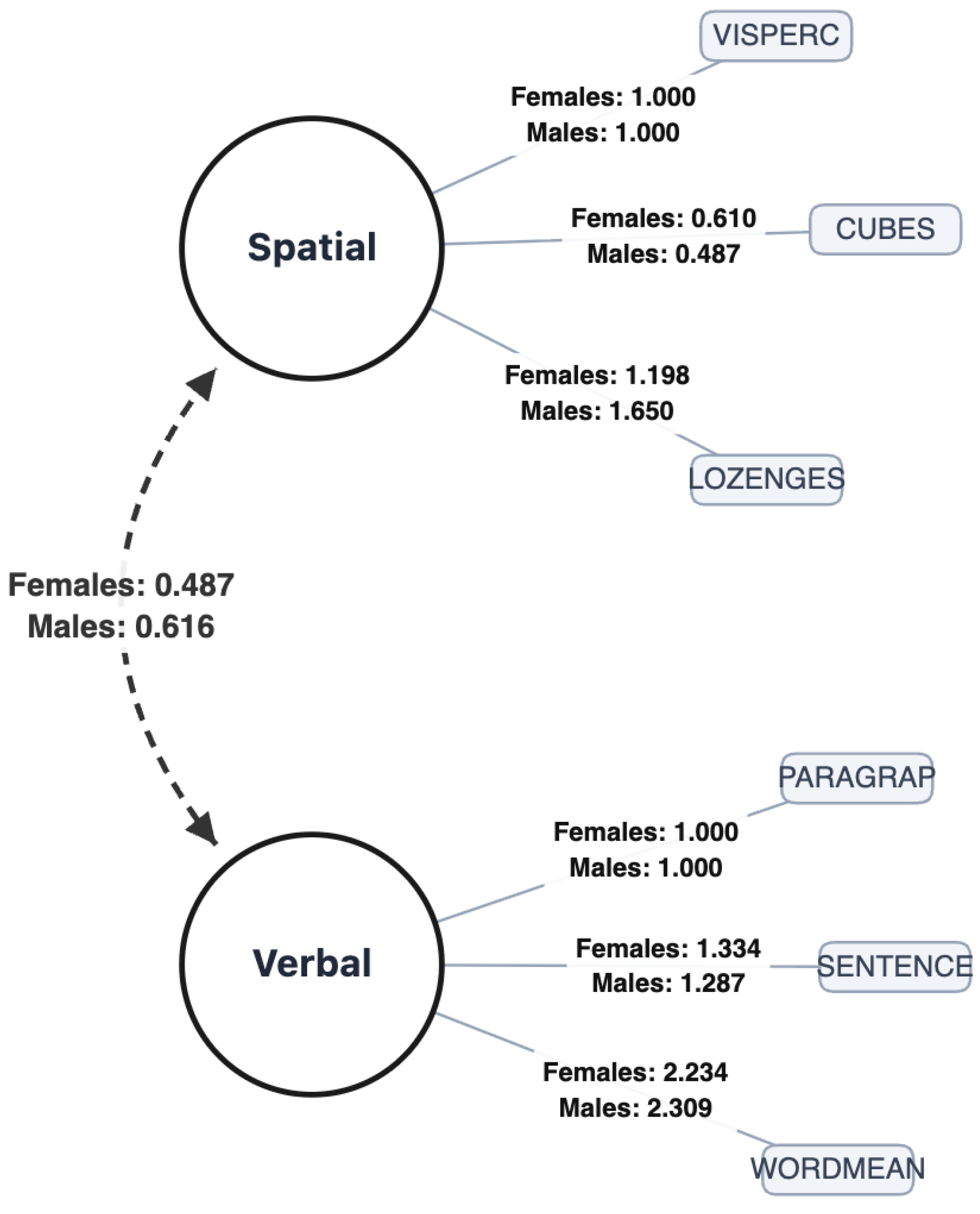
Figure 3.
SmartPLS 4 configural MGA diagrams — Females (left, n = 73) and Males (right, n = 72). Unstandardized loadings shown.
Figure 3.
SmartPLS 4 configural MGA diagrams — Females (left, n = 73) and Males (right, n = 72). Unstandardized loadings shown.
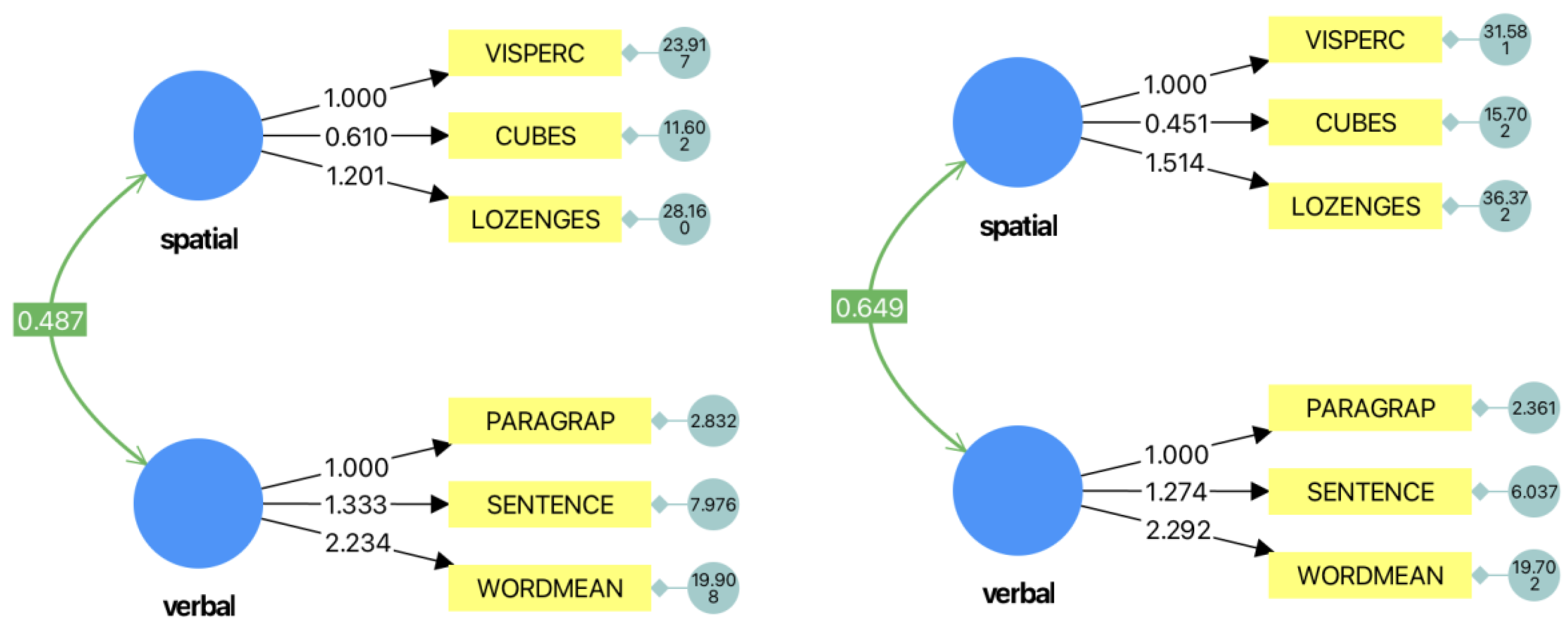
Figure 4.
LGCM path diagrams — AnalyVa (left) and SmartPLS 4 (right). Standardized loadings, inter-factor correlation (.580), and error variances shown (n = 400).
Figure 4.
LGCM path diagrams — AnalyVa (left) and SmartPLS 4 (right). Standardized loadings, inter-factor correlation (.580), and error variances shown (n = 400).
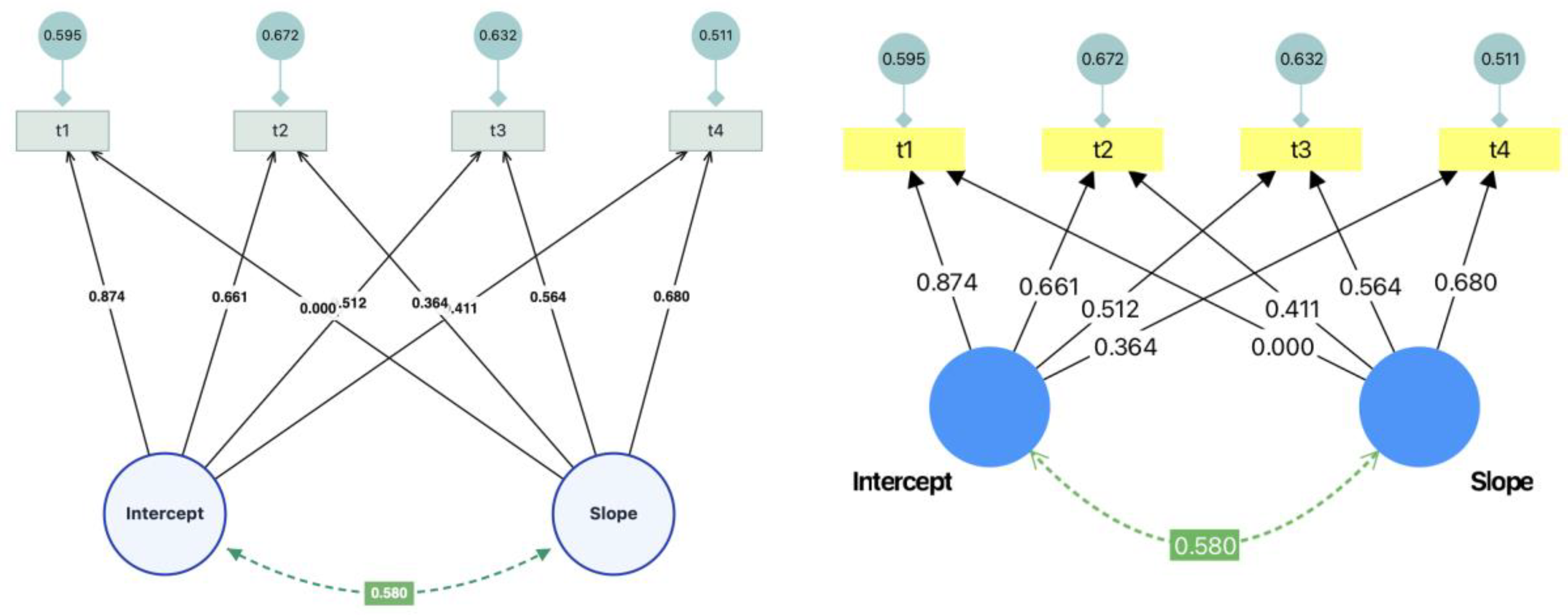
Figure 5.
Baseline OLS regression without copula term — SmartPLS 4 (left) and AnalyVa (right). Unstandardized path coefficients shown; R² = .976; n = 500.
Figure 5.
Baseline OLS regression without copula term — SmartPLS 4 (left) and AnalyVa (right). Unstandardized path coefficients shown; R² = .976; n = 500.
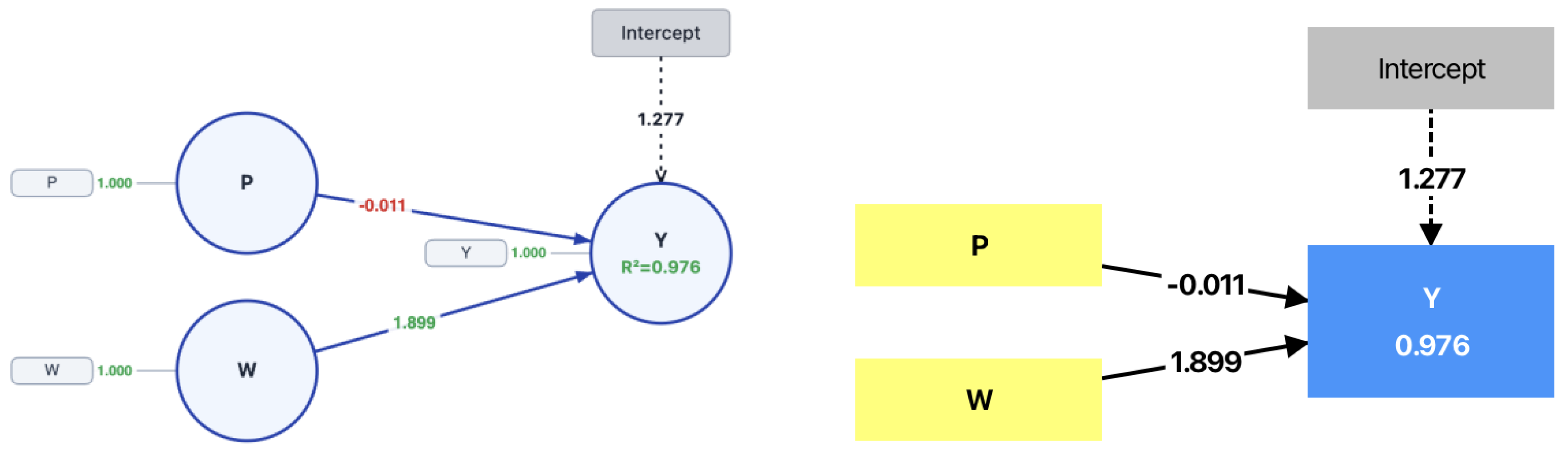
Figure 6.
Copula-corrected OLS regression with GC(P → Y) term — SmartPLS 4 (left) and AnalyVa (right). Unstandardized path coefficients shown; R² = .979; n = 500.
Figure 6.
Copula-corrected OLS regression with GC(P → Y) term — SmartPLS 4 (left) and AnalyVa (right). Unstandardized path coefficients shown; R² = .979; n = 500.
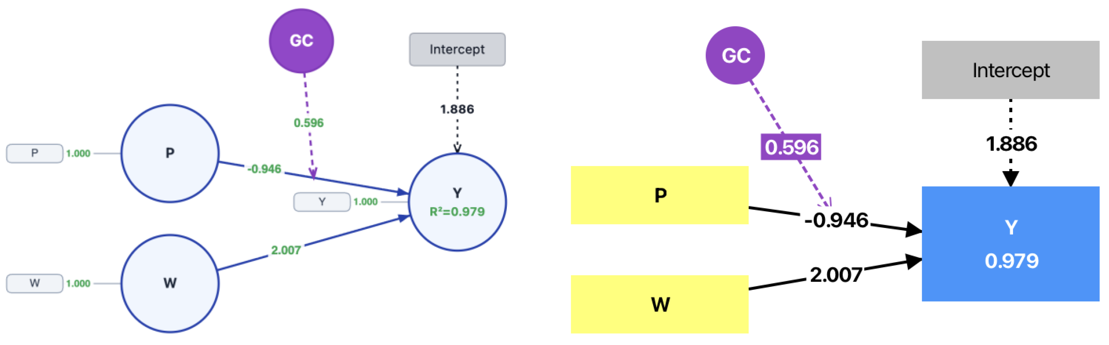
Figure 7.
Gaussian copula-augmented PLS-SEM — SmartPLS 4 (left) and AnalyVa (right). Purple nodes = GC copula terms (n = 344).
Figure 7.
Gaussian copula-augmented PLS-SEM — SmartPLS 4 (left) and AnalyVa (right). Purple nodes = GC copula terms (n = 344).
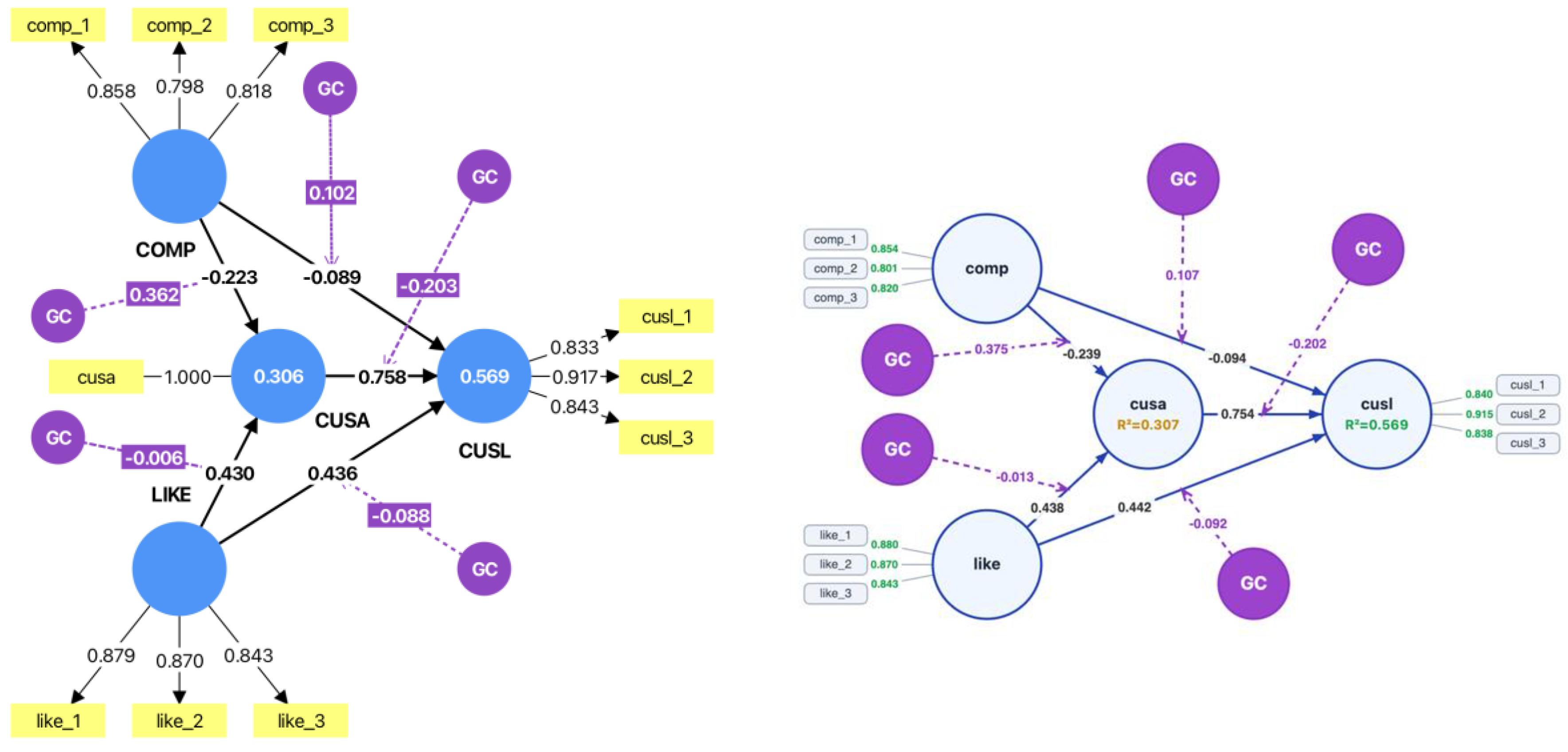

Table 1.
Study 1: Standardized Factor Loadings — AnalyVa vs. SmartPLS 4.
| Construct | Indicator | AnalyVa | SmartPLS 4 | |Δ| | Status |
| Spatial | visperc | .7029 | .7024 | .0005 | Accept |
| cubes | .6539 | .6538 | .0001 | Accept | |
| lozenges | .7362 | .7369 | .0007 | Good | |
| Verbal | paragrap | .8796 | .8797 | .0001 | Good |
| sentence | .8269 | .8270 | .0001 | Good | |
| wordmean | .8415 | .8414 | .0001 | Good | |
| MAD | .0003 |
Note. All loadings are standardized (ML estimation). Good = ≥ .70; Accept = .60–.69 (Hair et al., 2019). MAD < .001 = excellent concordance.
Table 2.
Study 1: Construct Reliability and Validity — AnalyVa vs. SmartPLS 4.
| Construct | Source | α | CR | AVE | AVE ≥ .50? |
| Spatial | AnalyVa | .742 | .742 | .488 | No (marginal) |
| SmartPLS 4 | .742 | .742 | .487 | No (marginal) | |
| Verbal | AnalyVa | .886 | .868 | .722 | Yes |
| SmartPLS 4 | .886 | .868 | .722 | Yes | |
| MAD | .000 | .000 | .001 |
Note. α = Cronbach’s alpha; CR = composite reliability (rho_c); AVE = average variance extracted. Thresholds: α ≥ .70, CR ≥ .70, AVE ≥ .50. HTMT(Spatial–Verbal): AnalyVa = .487, SmartPLS 4 = .476 (|Δ| = .011); both < .85 threshold.
Table 3.
Study 1: Global Model Fit Indices — AnalyVa vs. SmartPLS 4.
| Index | AnalyVa | Threshold | Status | SP4 Combined | |Δ| |
| χ²(8) | 7.962 | p > .05 | Good | 16.711 | — |
| p | .437 | > .05 | Good | .405 | — |
| χ²/df | .982 | < 3 | Good | 1.044 | .062 |
| RMSEA | .000 | ≤ .06 | Good | .018 | .018 |
| CFI | 1.000 | ≥ .95 | Good | .998 | .002 |
| TLI | 1.000 | ≥ .95 | Good | .996 | .004 |
| NFI | .958 | ≥ .90 | Good | .951 | .007 |
| SRMR | .043 | ≤ .08 | Good | .045 | .002 |
| AGFI | .889 | ≥ .90 | Marginal | .908 | .019 |
Note. AnalyVa fit: female subsample (n = 73). SP4 Combined: SmartPLS 4 configural MGA (n = 145). AGFI < .90 expected with small n. MAD across comparable indices = .007.
Table 4.
Study 2: Configural MGA Model Fit — AnalyVa vs. SmartPLS 4.
| Group / Model | n | χ² | df | CFI | TLI | RMSEA | SRMR |
| AnalyVa — Females | 73 | 7.962 | 8 | 1.000 | 1.000 | .000 | .043 |
| AnalyVa — Males | 72 | 8.748 | 8 | .994 | .990 | .036 | .047 |
| AnalyVa — Combined | 145 | 16.710 | 16 | .998 | .996 | .025 | .045 |
| SmartPLS 4 — Combined | 145 | 16.711 | 16 | .998 | .996 | .018 | .045 |
| |Δ| Combined | .001 | .000 | .000 | .007 | .000 |
Note. Configural model: same factor structure, freely estimated parameters within each group. SmartPLS 4 reports combined fit only.
Table 5.
Study 2: Group-Level Unstandardized Factor Loadings — AnalyVa vs. SmartPLS 4.
| Construct | Indicator | A-Fem | SP-Fem | A-Male | SP-Male | |Δ|F | |Δ|M |
| Spatial | visperc | 1.000 | 1.000 | 1.000 | 1.000 | .000 | .000 |
| cubes | 0.610 | 0.610 | 0.450 | 0.451 | .000 | .001 | |
| lozenges | 1.198 | 1.203 | 1.510 | 1.515 | .005 | .005 | |
| Verbal | paragrap | 1.000 | 1.000 | 1.000 | 1.000 | .000 | .000 |
| sentence | 1.334 | 1.335 | 1.275 | 1.276 | .001 | .001 | |
| wordmean | 2.234 | 2.235 | 2.294 | 2.295 | .001 | .001 | |
| MAD | .001 | .001 |
Note. A = AnalyVa; SP = SmartPLS 4; Fem = Females (n = 73); Male = Males (n = 72). First indicator per factor fixed to 1.0 (identification constraint).
Table 6.
Study 3: LGCM Standardized Factor Loadings — AnalyVa vs. SmartPLS 4.
| Time | Factor | Fixed λ | AnalyVa Std. λ | SP4 Std. λ | |Δ| | Concordance |
| t1 | Intercept | 1 | .8745 | .8745 | .0000 | Perfect |
| t1 | Slope | 0 | .0000 | .0000 | .0000 | Perfect |
| t2 | Intercept | 1 | .6608 | .6608 | .0000 | Perfect |
| t2 | Slope | 1 | .3641 | .3641 | .0000 | Perfect |
| t3 | Intercept | 1 | .5117 | .5117 | .0000 | Perfect |
| t3 | Slope | 2 | .5638 | .5638 | .0000 | Perfect |
| t4 | Intercept | 1 | .4112 | .4112 | .0000 | Perfect |
| t4 | Slope | 3 | .6797 | .6797 | .0000 | Perfect |
| MAD | .0000 |
Note. Std. λ = standardized factor loading. Fixed λ values are specified by construction and identical by design. MAD = .0000 = exact four-decimal-place agreement.
Table 7.
Study 3: Growth Factor Variances and Covariances — AnalyVa vs. SmartPLS 4.
| Parameter | AnalyVa | SmartPLS 4 | |Δ| | Concordance |
| Intercept variance | 1.9330 | 1.9330 | .0000 | Perfect |
| Slope variance | 0.5868 | 0.5868 | .0000 | Perfect |
| Intercept–Slope covariance | 0.6177 | 0.6177 | .0000 | Perfect |
| Intercept–Slope correlation | 0.5800 | 0.5800 | .0000 | Perfect |
Note. MAD = .0000 across all four parameters. Positive covariance (.618) indicates higher initial status predicts faster growth (cumulative advantage pattern).
Table 8.
Study 3: LGCM Global Model Fit — AnalyVa vs. SmartPLS 4.
| Index | AnalyVa | SmartPLS 4 | |Δ| | Threshold | Status | Concordance |
| χ²(3) | 5.421 | 5.421 | .000 | — | — | Perfect |
| p | .143 | .143 | .000 | > .05 | Accept | Perfect |
| RMSEA | .045 | .045 | .000 | ≤ .06 | Good | Perfect |
| SRMR | .008 | .008 | .000 | ≤ .08 | Good | Perfect |
| CFI | .999 | .999 | .000 | ≥ .95 | Good | Perfect |
| TLI | .997 | .997 | .000 | ≥ .95 | Good | Perfect |
| AGFI | .978 | .978 | .000 | ≥ .90 | Good | Perfect |
Note. All indices identical between platforms (MAD = .000). Model identified with df = 3, n = 400, providing adequate statistical power.
Table 9.
Study 4: Baseline OLS Regression (No Copula) — AnalyVa vs. SmartPLS 4.
| Predictor | Unstd. B | Std. β | SE | t | p | VIF | MAD |
| Intercept | 1.277 | 0.000 | .065 | 19.70 | < .001 | — | .000 |
| P | −0.011 | −0.002 | .052 | 0.208 | = .835 | 1.212 | .000 |
| W | 1.899 | 0.989 | .015 | 130.36 | < .001 | 1.212 | .000 |
Note. R² = .976, Adj. R² = .976, F(2,497) = 10,286, p < .001. Results identical between AnalyVa and SmartPLS 4 (MAD = .000 across all parameters).
Table 10.
Study 4: Copula-Corrected OLS Regression — AnalyVa vs. SmartPLS 4.
| Predictor | Unstd. B | Std. β | SE | t | p | VIF | |Δ| |
| Intercept | 1.886 | 0.000 | .106 | 17.763 | < .001 | — | .000 |
| P | −0.946 | −0.137 | .142 | 6.676 | < .001 | 9.739 | .000 |
| W | 2.007 | 1.045 | .021 | 96.875 | < .001 | 2.693 | .000 |
| GC(P→Y) | 0.596 | 0.131 | .084 | 7.053 | < .001 | 8.035 | .000 |
Note. R² = .979, Adj. R² = .978, F(3,496) = 7,546.68, p < .001. GC(P→Y) significant confirms endogeneity of P. MAD = .000 across all parameters. Durbin-Watson = 1.949 (both platforms).
Table 11.
Study 5: Outer Loadings — AnalyVa vs. SmartPLS 4 (Copula PLS-SEM).
| Construct | Indicator | AnalyVa λ | SP4 λ | |Δ| | ||
| COMP | comp_1 | .854 | .858 | .004 | ||
| comp_2 | .801 | .799 | .002 | |||
| comp_3 | .820 | .818 | .002 | |||
| LIKE | like_1 | .880 | .879 | .001 | ||
| like_2 | .870 | .870 | .000 | |||
| like_3 | .843 | .843 | .000 | |||
| CUSL | cusl_1 | .840 | .833 | .007 | ||
| cusl_2 | .915 | .917 | .002 | |||
| cusl_3 | .838 | .843 | .005 | |||
| MAD (λ) | .003 |
Note. MAD = .003 on outer loading magnitudes. All λ ≥ .70. Reliability MAD ≤ .001 (α, rho_c, AVE near-identical across platforms).
Table 12.
Study 5: Structural Path Coefficients and VIF — AnalyVa vs. SmartPLS 4.
| Path | AnalyVa β4. | SP4 β | |Δ| | Inner VIF | Interpretable? |
| LIKE → CUSA | .438 | .430 | .008 | 17.08 | Caution |
| CUSA → CUSL | .754 | .758 | .004 | 11.46 | Caution |
| LIKE → CUSL | .442 | .436 | .006 | 17.43 | Caution |
| COMP → CUSA | −.239 | −.223 | .016 | 16.56 | Caution |
| COMP → CUSL | −.094 | −.089 | .005 | 17.61 | Caution |
| GC(COMP→CUSA) | .375 | .362 | .013 | 16.31 | Caution |
| GC(COMP→CUSL) | .107 | .102 | .005 | 17.84 | Caution |
| GC(CUSA→CUSL) | −.202 | −.203 | .001 | 11.82 | Caution |
| GC(LIKE→CUSA) | −.013 | −.006 | .007 | 16.97 | Caution |
| GC(LIKE→CUSL) | −.092 | −.088 | .004 | 17.07 | Caution |
Note. Inner VIF values are near-identical across AnalyVa and SmartPLS 4 (VIF MAD ≤ .01 across all ten paths). VIF < 5 = acceptable; ≥ 5 = elevated; ≥ 10 = high (present study: 11–18 on both platforms; coefficients remain stable and comparable). R²: CUSA .307 vs. .306 (|Δ| = .001); CUSL .569 vs. .569 (|Δ| = .000).
Disclaimer/Publisher’s Note: The statements, opinions and data contained in all publications are solely those of the individual author(s) and contributor(s) and not of MDPI and/or the editor(s). MDPI and/or the editor(s) disclaim responsibility for any injury to people or property resulting from any ideas, methods, instructions or products referred to in the content. |
© 2026 by the authors. Licensee MDPI, Basel, Switzerland. This article is an open access article distributed under the terms and conditions of the Creative Commons Attribution (CC BY) license (http://creativecommons.org/licenses/by/4.0/).
Copyright: This open access article is published under a Creative Commons CC BY 4.0 license, which permit the free download, distribution, and reuse, provided that the author and preprint are cited in any reuse.