

Submitted:
16 July 2026
Posted:
29 July 2026
You are already at the latest version
Abstract
(1) Background: Characterizing causal structures in multivariate time series is a central challenge across neuroscience, economics, and environmental sciences; classical estimators identify which causal relations exist but lack compact descriptors capable of detecting how these relations organize themselves topologically over time. (2) Methods: We propose a multimodal framework that integrates sliding-window Granger causality estimation, the Vector Visibility Graph (VVG) representation, and three complementary topological descriptors—betweenness centrality, the Network Laplacian Spectral Descriptor (NetLSD), and the Deterministic Tourist Walk (DTW). The framework is evaluated on synthetic coupled autoregressive processes, coupled chaotic logistic maps, and a real-world case study with meteorological and rice price data from Uruguaiana, Brazil. (3) Results: Despite their mathematical independence, the three descriptors consistently identify a common critical coupling threshold λ∗ ≈ 0.9–1.0, providing internal cross-validation of the methodology. Experiments reveal pronounced topological reorganization near the synchronization regime, including attractor collapse, abrupt regime transitions detectable via bimodal degree distributions, and changes in graph connectivity patterns. The real-world case study demonstrates perfect non-parametric separation between distinct meteorological combinations. (4) Conclusions: The proposed multimodal framework provides interpretable, compact, and statistically robust topological descriptors of dynamic causal networks, complementing existing causal discovery methods.
Keywords:
topological network characterization
; multivariate time series
; complex networks
; visibility graphs
; deterministic tourist walk
; graph spectral descriptor
; Granger causality
1. Introduction
Internet-connected devices, social networks, and IoT sensors have generated massive volumes of multivariate time series. Their joint dynamics, capturing variables such as pressure and humidity together with temperature, provides a richer view of complex phenomena than univariate series alone [1,2].
Characterizing causal structures in multivariate time series has become a central challenge in neuroscience, economics, and environmental sciences. Classical methods such as Granger causality [3] provide estimators for the presence and direction of causal relations, yet the direct interpretation of the resulting p-value matrices is difficult in high-dimensional or non-stationary regimes [4,5], and these methods do not by themselves offer compact descriptors capable of detecting regime transitions or comparing causal structures over time [6,7].
The method proposed here does not aim to compete with consolidated causal discovery methods (Transfer Entropy [8], PCMCI [9], Convergent Cross Mapping [10], neural-network-based approaches [11,12]), but rather to complement them: while these estimators aim to identify which causal relations exist, our pipeline characterizes how these relations organize themselves topologically over time. We unify: (i) sliding-window estimation of Granger causality matrices, (ii) their transformation into complex networks via the Vector Visibility Graph (VVG) [13,14], and (iii) the analysis of these networks through three coordinated descriptors: betweenness centrality [15] captures local mediating structure; NetLSD [16] provides a global spectral view; and the Deterministic Tourist Walk (DTW) characterizes long-term dynamics through attractors and basins. We show that, although mathematically independent, these descriptors converge to a common critical threshold, providing an internal cross-validation that substitutes for comparison with external baselines in the specific task of topological characterization.
The remainder of the paper is organized as follows. The rest of Section 1 introduces the theoretical building blocks (Granger causality, VVG, betweenness centrality, NetLSD, and DTW). Section 2 reviews related work. Section 3 describes the methodology. Section 4 reports synthetic and real-data results, and Section 6 concludes.
1.1. Granger Causality
Granger causality (GC) formalizes the predictive influence between time series: is said to Granger-cause if past values of provide statistically significant information for predicting beyond what is already contained in the past of [3]. Considering two stochastic signals modeled as univariate autoregressions , for , with the corresponding bivariate models
Granger-causes if the cross-coefficients are jointly different from zero. The null hypothesis is tested through a nested F-test, , where and are the residual sums of squares of the restricted and unrestricted models, is the number of restrictions, T the sample size, and k the number of parameters of the unrestricted model. We adopt and select the lag order p via the Bayesian Information Criterion (BIC) [17].
1.2. Vector Visibility Graph
The Vector Visibility Graph extends the classical visibility graph to multivariate series, mapping them onto a directed complex network [13,14]. Given a series , , each vector is a node. The projection of onto () is . The vectors and have directed visibility if, for every c such that ,
Geometrically, is visible from if no intermediate vector dominates the line of sight, where the obstruction is measured by the scalar projection of each vector onto the direction of . Time instants with similar and persistent causal structures tend to be mutually visible, forming hubs of high connectivity. All topological metrics below are computed on the underlying undirected version of the VVG, since the objective is to characterize the intensity and structure of causal coupling rather than its direction.
1.3. Betweenness Centrality
Betweenness centrality [15] quantifies the importance of a node v along the shortest paths of the network: , with the number of shortest paths between s and t and the number passing through v. For an undirected network with N nodes, the reference value adopted in this work is , the centrality of the hub in a canonical star topology.
1.4. Network Laplacian Spectral Descriptor (NetLSD)
NetLSD [16] is a permutation-invariant, size-invariant, and scale-adaptive spectral descriptor. Given with , the normalized Laplacian admits the spectral decomposition , with eigenvalues . The heat equation admits , and NetLSD uses the trace
sampled at logarithmically spaced . We normalize by the empty graph signature, with , and use the distance between normalized signatures. For each pair of coupling values and autoregressive coefficient , we compute the mean over independent realizations,
Diagonal elements () quantify intra-regime variability (spectral reproducibility); off-diagonal elements () quantify inter-regime discriminability. The heatmaps are normalized row-wise.
1.5. Deterministic Tourist Walk (DTW)
The DTW is a partially self-avoiding deterministic walk [18,19]. An agent departs from each node and moves following the maximum-degree rule
with . Ties are broken by node index; if all neighbors have already been visited, the tourist revisits the highest-degree neighbor, generating a limit cycle. Each trajectory splits into a transient phase and an attractor phase, characterized by the means and standard deviations of the transient and period , the number of unique attractors , and the dominance of the largest basin
High indicates structural coherence; low values indicate dynamical fragmentation.
2. Related Work
Complex networks offer a powerful framework to analyze time series and detect regime changes, characterize nonlinear dependencies, and quantify information flow [20,21,22,23]. Methods for time-varying causal networks include kernel reweighted group lasso for dynamic VAR models [24], dynamic graph structure learning [25], and spectral co-clustering on evolving directed graphs. Visibility graphs [13,14,20,26] and their multivariate and vector generalizations [6,7,27] bridge time series and network analysis, while NetLSD currently represents the state of the art in compact, invariant graph representation. Despite this variety, there is a lack of compact, interpretable topological descriptors capable of characterizing time-varying causal networks in a multimodal fashion. The proposed framework fills this gap by integrating sliding-window Granger estimation with the VVG and validating it through three complementary descriptors. The DTW, conceptually simple and discriminative, is employed here as a long-term dynamical descriptor, complementing NetLSD (spectral) and betweenness centrality (local). Table 1 summarizes the differentiation: the central axis is not the causal estimator (treated as an interchangeable input) but the multimodal topological analysis of the resulting networks.
3. Materials and Methods
Figure 1 shows the pipeline, structured in five stages: generation of time series, extraction of causality matrices via sliding windows, vectorization of the matrices, construction of the VVG, and topological analysis through the three descriptors.
3.1. Synthetic Time Series
3.1.1. Scenario A (Coupled AR(1) Chain)
Four series of length are generated by an AR(1) process with linear lagged coupling:
with i.i.d. We use and (20 values), yielding 80 combinations with independent simulations each (8,000 realizations). Initial values for are sampled from . The coefficient controls intrinsic memory ( produces white noise, large introduces strong autocorrelation), and regulates the coupling intensity along the chain. Figure 2 illustrates, for , the cases and . We also consider an abrupt change at : (i) and (ii) (Figure 2, right panels).
3.1.2. Scenario B (Coupled Chaotic Logistic Maps)
A bivariate experiment with coupled chaotic oscillators (the coupling constant is denoted to avoid notational collision):
with , , , and . For , in the deterministic case, the Lyapunov exponent of the logistic map is . Transverse stability of the synchronized solution requires , so that , with , i.e., [28,29]. In the presence of independent noise, synchronization becomes approximate, characterized by the reduction of the transverse error within this coupling range.
3.2. Sliding-Window Causal Vectors and VVG Construction
Within each window , the Granger causality p-value matrix is
and is linearized into . We tested and report for Scenario A (maximum sensitivity to ) and for Scenario B. The sequence defines the nodes of the VVG. A directed edge is created when satisfy Equation (2); the topological analysis uses the underlying undirected version.
3.3. Topological Descriptors and Validation
The aggregate measure of structural intensity is the normalized maximum betweenness centrality
with nodes (for , : , denominator ). For NetLSD, we compute Equation (4) for all triples with . For the DTW, a walk is initiated from every node following Equation (5), and the aggregate metrics are computed and averaged over the 100 realizations. All results are reported as means with standard error.
3.3.1. Computational Complexity
Let be the number of VVG nodes and E the number of edges. The Granger stage costs ; VVG construction is for sparse graphs (worst case ); Brandes’s betweenness algorithm [15] is ; the NetLSD spectral decomposition is in general, with Lanczos for sparse graphs; the DTW is , with the mean degree. For Scenario A (, , , ), one realization runs in 2–5 min on a single CPU core (Python); parallelization over the realizations scales linearly with the number of cores.
4. Results
4.1. Degree Distribution in Causal Networks
4.1.1. Scenario A
Figure 3 compares the VVG degree distributions with windows and for , contrasting and . With , the topological difference is immediate: the distribution is concentrated, with degrees typically below 200, while exhibits tails extending up to degrees of the order of the network size (∼5,000), indicating the emergence of giant hubs. In the VVG, the degree of a node t measures how many other instants can see the causal vector without geometric obstruction. For , vectors are dominated by noise and the visibility geometry is essentially random, consistent with VVGs from white-noise series [30]. For , the chain imprints persistent signatures on , and instants with pronounced causal structure become geometric reference points. When L is increased to 100, the two distributions become almost indistinguishable, signaling a loss of sensitivity. The window controls temporal resolution: small L preserves the variability of , while large L acts as a temporal low-pass filter, homogenizing and destroying topological discrimination. The choice is the empirical balance for Scenario A.
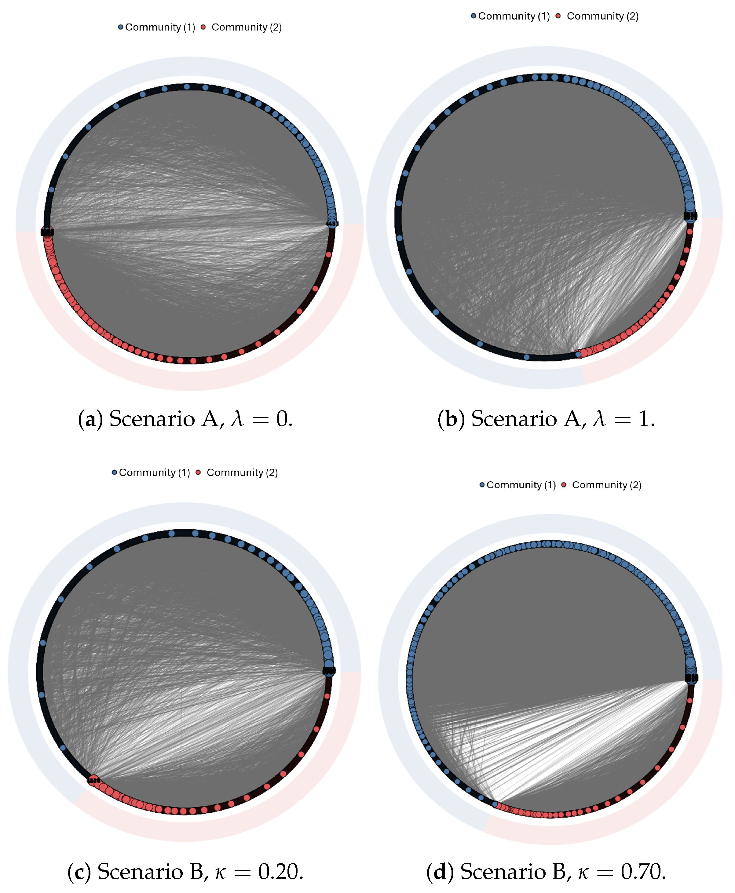
The circular visualization in Figure 6 (top) complements this analysis. Communities were identified by the Girvan–Newman algorithm [31]; in all analyzed cases the algorithm detected exactly two communities. For , communities are diffuse and weakly delimited; for , densely connected communities emerge with visible hubs near the inter-community boundary, acting as temporal bridges between weakly and strongly coupled segments of the series, consistent with recurrence-network results [20,21].
Figure 4 reveals one of the most expressive findings of this section: under an abrupt change at , the degree distribution is clearly bimodal, with one mode at degrees 5–8 (uncoupled segment) and another at 15–20 (coupled segment). This bimodality is absent in series of constant coupling and emerges precisely because the VVG simultaneously integrates causal vectors from two distinct regimes. Comparison with a purely stochastic series of the same duration (Figure 4b) confirms that the second mode is a robust structural signature rather than a fluctuation artifact, and Figure 4c shows that the bimodality disappears for due to temporal dilution. Practical implication: simple inspection of the degree distribution of the global VVG can signal a structural change without partitioning the series or specifying the change point a priori.
4.1.2. Scenario B
The coupled logistic maps offer a qualitatively distinct robustness test: deterministic and chaotic dynamics, with a precise theoretical synchronization threshold [28,29]. With (Figure 5), the contrast between the two regimes is even sharper than in Scenario A. For (outside the synchronization window), the distribution follows a power law typical of VVGs from non-synchronized chaotic series [30]. For (inside the synchronization window), the distribution becomes bimodal with a tail up to ∼2,000. When the maps synchronize, their states become essentially identical, the causal vectors converge to a stationary state of high coherence, and highly coherent vectors share nearly total mutual visibility, generating hubs. The bimodality is informative: the first mode reflects transient instants in which synchronization is partially broken by the noise , the second mode corresponds to instants of full synchronization, and the separation between them encodes the fraction of time spent in full synchronization. The circular visualizations (Figure 6, bottom) confirm this picture: for , a diffuse structure without hubs; for , high-connectivity hubs concentrated in a restricted region of the circle, forming a dense core of fully synchronized instants. Taken together, Scenarios A and B demonstrate that the degree distribution of the causal VVG is a robust topological discriminator sensitive both to the intensity of the coupling and to the underlying dynamical mechanism (linear vs. chaotic, stochastic vs. deterministic).
Figure 5.
VVG degree distribution with for coupled logistic maps. Blue: (synchronized); orange: (non-synchronized). The bimodal distribution with a tail up to ∼2,000 in the synchronized regime contrasts with the power-law distribution of the non-synchronized regime.
Figure 5.
VVG degree distribution with for coupled logistic maps. Blue: (synchronized); orange: (non-synchronized). The bimodal distribution with a tail up to ∼2,000 in the synchronized regime contrasts with the power-law distribution of the non-synchronized regime.
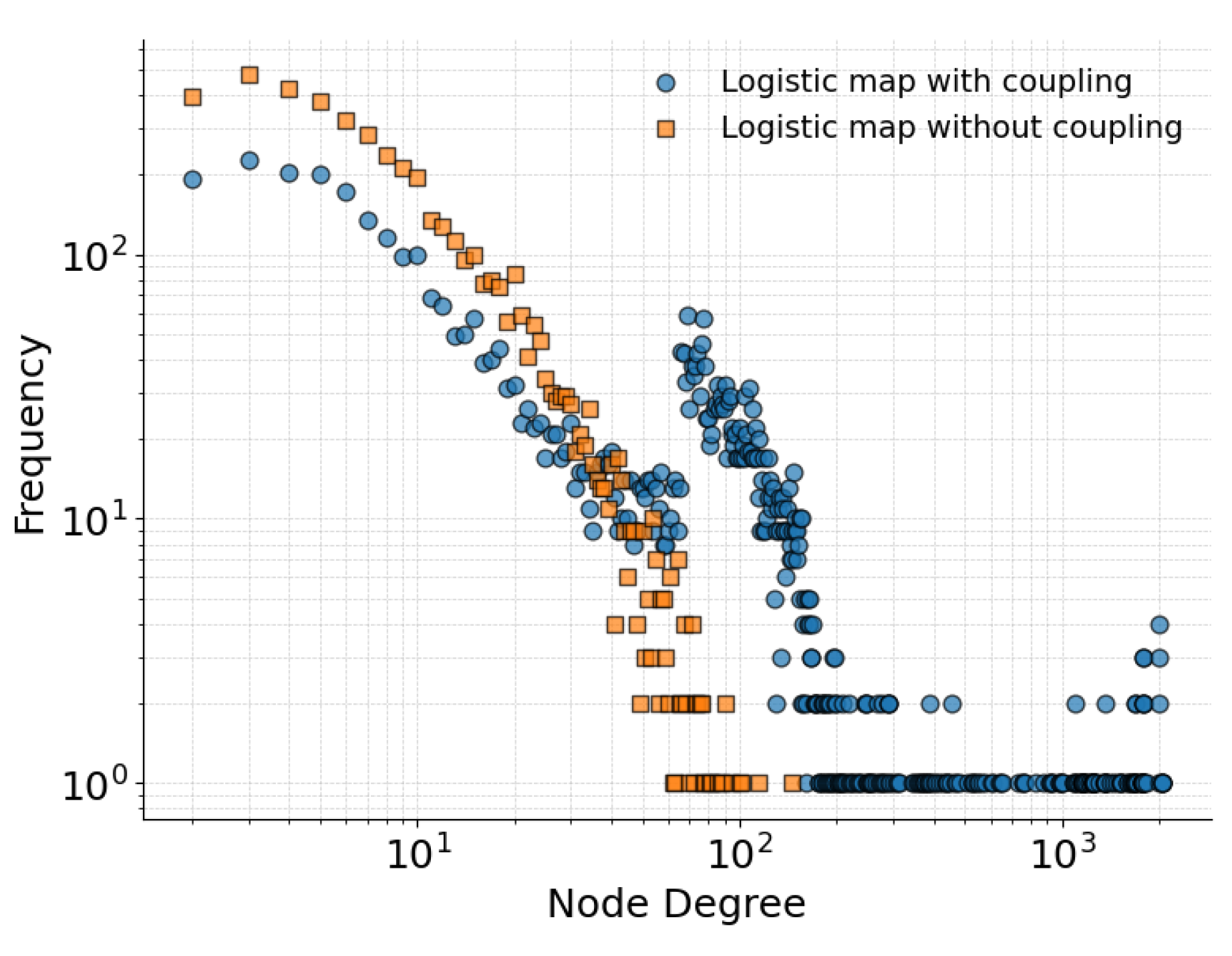
Figure 6.
Circular visualization of the VVG. Two communities detected by the Girvan–Newman algorithm [31] in all cases. (a) Scenario A with . (b) Scenario A with . (c) Scenario B with . (d) Scenario B with . Coupled/synchronized regimes (right column) show densely connected communities with visible inter-community hubs, absent in the uncoupled/non-synchronized regimes (left column).
Figure 6.
Circular visualization of the VVG. Two communities detected by the Girvan–Newman algorithm [31] in all cases. (a) Scenario A with . (b) Scenario A with . (c) Scenario B with . (d) Scenario B with . Coupled/synchronized regimes (right column) show densely connected communities with visible inter-community hubs, absent in the uncoupled/non-synchronized regimes (left column).
4.2. Structural Characterization via Betweenness Centrality
Figure 7 shows the normalized mean maximum betweenness centrality (Equation (10)) as a function of for the four values of . For each , the 100 trials are fitted by a saturated exponential
whose parameters and goodness-of-fit are reported in Table 2. The centrality grows from at to a saturation plateau , reflecting the competition between stochastic disorder (dominant for small , random visibility geometry, no dominant mediating nodes) and the hierarchical organization induced by the chain (dominant for large , instants of intense causal transmission become hubs).
All four coefficients yield and with , confirming that the fits are statistically compatible with the experimental errors. Comparison with a logistic sigmoid of the same number of parameters [32] shows that the exponential is preferable for ( and ; strong evidence) and statistically indistinguishable for ; in the latter cases, the saturated exponential is adopted for the interpretability of its parameters: is the topological saturation level, the total transition amplitude, and the rate of emergence of the causal signal over the noise. Both and decrease monotonically with (autoregressive memory distributes the causal signal more uniformly, attenuating topological concentration), while grows from 0.643 () to 1.840 (): autocorrelation increases the signal-to-noise ratio of the Granger estimator at fixed , accelerating the transition although the saturation level reached is lower. The standard error of c for is substantially larger () because saturation occurs rapidly and few observational points precede the plateau; the claim of monotonic growth of is therefore robust but with reduced certainty for the extreme value .
4.3. Spectral Validation: NetLSD
Figure 8 shows the heatmaps of the normalized mean distance between NetLSD signatures (Equation (4)) for and the four values of . For all , the heatmaps display a bipartite structure with a transition band that splits the parameter space into two qualitatively distinct blocks.
The red block corresponds to pairs with significant coupling difference, such as : VVGs generated in such distinct regimes exhibit markedly different spectral signatures, resulting in high distances and reflecting the sensitivity of NetLSD to the coupling constant. The blue block, in turn, corresponds to pairs whose coupling values are close to each other: since VVGs generated in similar regimes share the same dominant topological structure, their NetLSD signatures converge and the residual distances (∼0.09–0.22) are small, representing intrinsic variability between realizations rather than genuine structural difference. In particular, diagonal elements () quantify intra-regime spectral reproducibility. The transition band corresponds to the interval of over which the spectrum of the normalized Laplacian undergoes its largest reorganization, captured by the heat trace at multiple scales.
The threshold shifts monotonically: – for and , broadening for and shifting to – for . The residual distances in the blue block grow from 0.09–0.13 (low ) to 0.13–0.22 (). All heatmaps are approximately symmetric, consistent with the symmetry of the metric. The coincidence between this spectral threshold and the point at which betweenness centrality begins its systematic growth (Section 4.2) is a non-trivial coherence result and provides internal cross-validation of the method.
4.4. Dynamical Analysis via DTW
Figure 9a shows the mean transient as a function of . The pattern is non-monotonic: for all , decreases from , reaches a minimum in the range –, and recovers toward a plateau comparable to the baseline. For , drops from ∼170 at to at , recovering to ∼150–175 for . For the same pattern holds with globally suppressed values (minimum ∼70, plateau ∼90). A Wilcoxon test (Holm correction [33]) confirms the valley as significant only for , (, ); for the other , the pattern is consistent in the means but indistinguishable from noise at the individual-realization level, reflecting limited statistical power rather than absence of the phenomenon. The mechanistic interpretation is robust: at , the absence of hubs forces long walks; at moderate , incipient hubs quickly capture the tourist but are not yet globally connected, yielding short cycles and minimum transients; at , giant hubs dominate the topology and the tourist circulates in cycles involving them, raising back to the plateau.
Figure 9b shows the monotonic collapse of with two phases: rapid decay for and a plateau for . From –890 at (high dynamical fragmentation), progressively more connected hubs attract trajectories into a smaller set of limit cycles. The Kruskal–Wallis test on plateau points () strongly rejects equality between groups (, ), and pairwise Mann–Whitney comparisons with Holm correction (Table 3) confirm all six pairs as significantly distinct. This formally establishes that autoregressive memory preserves dynamical diversity even under strong causal coupling: each converges to a structurally distinct plateau, around 240–290 attractors for and 300–400 for —a result consistent with the role of autocorrelation in maintaining dynamically diverse trajectories even when the network topology is dominated by high-connectivity hubs.
Figure 9c shows the sigmoidal behavior of with three phases: low plateau (, no dominant attractor), abrupt growth around –, and a new plateau () whose level depends strongly on . Fitting a logistic yields (95% CI ) for , () for , () for , and () for . The CIs overlap and are compatible with for , formally confirming the convergence already identified by betweenness centrality and NetLSD. For , the fit returns with a CI including zero, indicating that the transition is already complete before the smallest in the grid and the sigmoidal fit loses resolution in this regime. The sigmoidal character of is a classical phase-transition signature [34], with the order parameter remaining small in the disordered phase and saturating in the ordered phase; its abrupt growth near is the dynamical counterpart of the centrality saturation.
Figure 9d integrates and in a single scatter plot, showing a quasi-orthogonal separation of (cluster position) and (displacement within cluster), useful for identifying the dynamical regime of an unknown real system from its position in this plane.
4.4.1. Internal Cross-Validation
The three descriptors converge into a coherent picture. First, the threshold – identified by NetLSD coincides with (a) the onset of systematic centrality growth ( for all , ) and (b) the sigmoidal inflection of , whose 95% CIs overlap among and contain . Shortest paths, Laplacian spectrum, and attractor basins formally point to the same critical point. Second, the U-shaped minimum of at – lies slightly below , consistent with the interpretation that this region precedes topological consolidation. Third, the effect of is quantitatively consistent and statistically confirmed across descriptors: monotonic reduction of and ; leftward shift of the NetLSD boundary; and significant distinction of all plateau pairs. This triple convergence (local, spectral, dynamical) constitutes the internal cross-validation of the framework, the most rigorous form of robustness evaluation available in the absence of established external baselines for the specific task of topological characterization.
4.5. Case Study: Meteorological Variables and Rice Prices
To illustrate applicability to real data, we conducted a case study on meteorological time series and rice prices in Southern Brazil during 2015–2025, using INMET data (https://portal.inmet.gov.br/dadoshistoricos, accessed on 1 March 2026) combined with CEPEA rice price series (https://www.cepea.org.br/br/consultas-ao-banco-de-dados-do-site.aspx, accessed on 1 March 2026) for Uruguaiana (RS), the country’s main rice-producing hub. The goal is to demonstrate the discriminative power of the topological characterization, not to claim discovery of causal drivers of rice prices.
The dataset comprises a multivariate series of 2,000 points. From the 17 available meteorological variables, all triplets were formed, each concatenated with the rice price series to produce a multivariate time series of dimension , matching Scenario A. The pipeline was applied to each of the 680 series independently. Combinations were ranked by and the top 15 (Top 15) and bottom 15 (Bottom 15) were retained for comparative analysis. The separation between groups is assessed by the DTW metrics ( and ), which are mathematically independent of betweenness centrality and did not enter the selection criterion; convergence of the three metrics is therefore non-trivial evidence.
Figure 10a shows the centrality profiles. The separation is sharp: Top 15 curves reach , while Bottom 15 stays below ∼0.10. The value 0.20 is consistent with the saturation plateau in Table 2, suggesting that the most prominent meteorological combinations induce an effective causal coupling of the order in the equivalent generating system. Figure 10b,c report and for the two groups. The separation was assessed via two-sided Mann–Whitney U tests: for , (, ); for , (, ). The value is the maximum possible for : every value of the Top 15 exceeds every value of the Bottom 15 with no overlap. Perfect separation in two metrics independent of the ranking criterion establishes that the discrimination is not an artifact of selection but a coherent structural property of the framework on real data.
Table 4 reports the frequency of meteorological variables in the two groups. The asymmetry is marked: Top 15 is dominated by minimum relative humidity, atmospheric pressure (maximum, minimum, and station-level), and wind variables (direction and speed). This set is consistent with the influence of synoptic-scale atmospheric systems, such as cold fronts, extratropical cyclones, and post-frontal anticyclones, which periodically modulate meteorological conditions during the rice growing season (October to March). In this context, atmospheric pressure should be interpreted as an indirect indicator of the passage and reorganization of these systems, while wind and relative humidity capture changes in advection, atmospheric stability, and evaporative demand. The association between high-pressure systems and evapotranspiration, however, depends on the thermal regime, humidity, radiation, and wind; therefore, their effects on irrigation costs and grain quality must be interpreted conditionally [35,36,37].
Bottom 15 is dominated by total precipitation, minimum temperature, and hourly relative humidity. The lower frequency of these variables is compatible with the specificity of flood-irrigated lowland rice in Uruguaiana, whose water availability is strongly mediated by irrigation management, reducing direct dependence on local precipitation compared to rainfed systems. Thus, the topological separation suggests a plausible regional agronomic signature [38], rather than an arbitrary methodological choice. We do not claim causality in the econometric sense; such inference would require explicit control of confounding variables—including international prices, exchange rates, agricultural policies, and management decisions—in addition to dedicated time-series modeling.
5. Discussion
The results presented above support a coherent interpretation of the proposed framework. The convergence of three mathematically independent descriptors (betweenness centrality, NetLSD, and DTW) toward a common critical threshold – in Scenario A is the central finding: it shows that the topological reorganization of the causal VVG near the coupling-induced transition is not an artifact of a single metric but a genuine structural property captured from local, spectral, and dynamical perspectives simultaneously. The systematic leftward shift of as increases admits a physically interpretable explanation: autoregressive memory increases the effective signal-to-noise ratio of the Granger estimator at fixed , anticipating the topological consolidation; the same mechanism explains the monotonic growth of in the centrality fit and the reduction of the saturation level , since memory distributes the causal signal more uniformly across time.
The detection of regime transitions through bimodality in the global VVG degree distribution offers a practical advantage over methods that require a priori specification of change points. Together with the chaotic-map experiments, which confirm consistency with the theoretical synchronization threshold , this suggests that the framework is sensitive to the underlying dynamical mechanism rather than to the specific functional form of the coupling. The Uruguaiana case study illustrates that this sensitivity extends to real data: the perfect non-parametric separation between Top 15 and Bottom 15 across three independent metrics shows that the topological discrimination is structural rather than a selection artifact, and the agronomic plausibility of the most frequent variables in each group lends external coherence to the analysis.
Several limitations should be acknowledged. First, the framework treats the causal estimator as an interchangeable input; while Granger causality is convenient and well understood, regimes with strong nonlinearity or non-Gaussian noise may require alternatives such as Transfer Entropy [8] or PCMCI [9], whose interaction with the VVG and the three descriptors deserves dedicated investigation. Second, the choice of the sliding window L is empirically tuned and exhibits a clear bias–variance trade-off: small L preserves topological discrimination but increases variability, while large L acts as a temporal low-pass filter; principled criteria for window selection in nonstationary settings remain an open direction [39]. Third, the real-data analysis is illustrative rather than confirmatory; rigorous causal inference on rice prices would require explicit control of confounders such as international prices, exchange rates, and agricultural policies. Future work includes extending the framework to higher-dimensional series, replacing Granger with nonlinear causal estimators, and exploring the convergence of additional topological descriptors (e.g., persistent homology [40,41] and graph wavelets).
6. Conclusions
We introduced a unified method for the multimodal topological characterization of dynamic causal networks built from multivariate time series, integrating sliding-window Granger estimation, the Vector Visibility Graph, and three complementary topological descriptors (betweenness centrality, NetLSD, DTW) into a coherent and interpretable pipeline. The framework does not compete with consolidated causal discovery methods such as PCMCI, Transfer Entropy, and CCM, but complements them: while these estimators aim to identify which causal relations exist, our pipeline characterizes how these relations organize topologically over time.
The central result is the convergence of three mathematically independent perspectives—shortest-path distribution (centrality), normalized Laplacian spectrum (NetLSD), and attractor-basin distribution (DTW)—to a common critical threshold – for low , with a systematic leftward shift as increases. This triple convergence constitutes an internal cross-validation of the framework: in the absence of established external baselines for the specific task of topological characterization of dynamic causal networks, the mutual coherence of three independent metrics is the most rigorous form of robustness evaluation available. Quantitatively, the normalized maximum betweenness centrality is well described by a saturated exponential , whose parameters encode the competition between autoregressive memory and external coupling in an interpretable manner.
The framework also detects regime transitions passively (without partitioning the series): the abrupt change at produces a bimodal degree distribution whose two modes correspond to the two coupling regimes. Scenario B (coupled chaotic logistic maps) confirms consistency with the theoretical synchronization threshold , showing that the framework is sensitive to the underlying dynamical mechanism (linear vs. chaotic, stochastic vs. deterministic). The case study using INMET meteorological data and CEPEA rice prices for Uruguaiana (2015–2025) demonstrated perfect topological separation between Top 15 and Bottom 15 across the three metrics, with variables associated with the Top 15 plausible in light of regional agronomic literature.
Author Contributions
Conceptualization, F.P.A. and L.Z.; methodology, F.P.A. and L.Z.; software, F.P.A.; validation, F.P.A.; formal analysis, F.P.A.; investigation, F.P.A.; data curation, F.P.A.; writing—original draft preparation, F.P.A.; writing—review and editing, F.P.A. and L.Z.; supervision, L.Z.; funding acquisition, L.Z. All authors have read and agreed to the published version of the manuscript.
Funding
This work is partially supported by the São Paulo Research Foundation (FAPESP) through Grants #2019/07665-4 and #2024/15430-5, and by the Brazilian National Council for Scientific and Technological Development (CNPq) through Grants #406417/2022-9, #306788/2023-3 and #403307/2025-2.
Institutional Review Board Statement
Not applicable.
Informed Consent Statement
Not applicable.
Data Availability Statement
The raw data and source code supporting the conclusions of this article are available from the corresponding author upon reasonable request. The meteorological data used in the case study are publicly available from the Brazilian National Institute of Meteorology (INMET) at https://portal.inmet.gov.br/dadoshistoricos (accessed on 1 March 2026), and the rice price data are publicly available from the Center for Advanced Studies in Applied Economics (CEPEA) at https://www.cepea.org.br/br/consultas-ao-banco-de-dados-do-site.aspx (accessed on 1 March 2026). Synthetic data can be reproduced from the parameter specifications and equations provided in Section 3.
Acknowledgments
The authors acknowledge the Institute of Mathematics and Computer Sciences (ICMC) at the University of São Paulo for the computational infrastructure used in this study.
Conflicts of Interest
The authors declare no conflicts of interest. The funders had no role in the design of the study; in the collection, analyses, or interpretation of data; in the writing of the manuscript; or in the decision to publish the results.
Abbreviations
The following abbreviations are used in this manuscript:
| AIC | Akaike Information Criterion |
| AR | Autoregressive |
| BIC | Bayesian Information Criterion |
| CCM | Convergent Cross Mapping |
| CEPEA | Center for Advanced Studies in Applied Economics |
| CI | Confidence Interval |
| DTW | Deterministic Tourist Walk |
| GC | Granger Causality |
| INMET | Brazilian National Institute of Meteorology |
| NetLSD | Network Laplacian Spectral Descriptor |
| PCMCI | Peter and Clark Momentary Conditional Independence |
| VAR | Vector Autoregression |
| VVG | Vector Visibility Graph |
References
- Esling, P.; Agon, C. Time-series data mining. ACM Comput. Surv. 2012, 45, 1–34. [Google Scholar] [CrossRef]
- Yang, D.; Chen, H.; Song, Y.; Gong, Z. Granger Causality for Multivariate Time Series Classification. In Proceedings of the 2017 IEEE International Conference on Big Knowledge (ICBK); IEEE, 2017; pp. 103–110. [Google Scholar] [CrossRef]
- Granger, C.W.J. Investigating causal relations by econometric models and cross-spectral methods. Econometrica 1969, 37, 424–438. [Google Scholar] [CrossRef]
- Cheng, Y.; Yang, R.; Xiao, T.; Li, Z.; Suo, J.; He, K.; Dai, Q. CUTS: Neural Causal Discovery from Irregular Time-Series Data. In Proceedings of the Eleventh International Conference on Learning Representations (ICLR), 2023. [Google Scholar] [CrossRef]
- Placek, M.M.; Beqiri, E.; Czosnyka, M.; Smielewski, P. Technical considerations on the use of Granger causality in neuromonitoring. Brain Multiphysics 2022, 3, 100044. [Google Scholar] [CrossRef]
- Jiang, M.; Gao, X.; An, H.; Li, H.; Sun, B. Reconstructing complex network for characterizing the time-varying causality evolution behavior of multivariate time series. Sci. Rep. 2017, 7, 10486. [Google Scholar] [CrossRef] [PubMed]
- Carlos-Sandberg, L.; Clack, C. Incorporation of causality structures to complex network analysis of time-varying behaviour of multivariate time series. Sci. Rep. 2021, 11, 18880. [Google Scholar] [CrossRef] [PubMed]
- Schreiber, T. Measuring information transfer. Phys. Rev. Lett. 2000, 85, 461–464. [Google Scholar] [CrossRef] [PubMed]
- Runge, J. Discovering contemporaneous and lagged causal relations in autocorrelated nonlinear time series datasets. In Proceedings of the 36th Conference on Uncertainty in Artificial Intelligence (UAI); PMLR, 2020; Vol. 124, pp. 1388–1397. [Google Scholar]
- Sugihara, G.; May, R.; Ye, H.; Hsieh, C.; Deyle, E.; Fogarty, M.; Munch, S. Detecting causality in complex ecosystems. Science 2012, 338, 496–500. [Google Scholar] [CrossRef] [PubMed]
- Tank, A.; Covert, I.; Foti, N.; Shojaie, A.; Fox, E.B. Neural Granger causality. IEEE Trans. Pattern Anal. Mach. Intell. 2022, 44, 4267–4279. [Google Scholar] [CrossRef] [PubMed]
- Hasan, U.; Hossain, E.; Gani, M.O. A survey on causal discovery methods for I.I.D. and time series data. Transactions on Machine Learning Research 2024. Available online: https://openreview.net/forum?id=YdMrdhGx9y. [CrossRef]
- Ren, W.; Jin, N. Vector visibility graph from multivariate time series: A new method for characterizing nonlinear dynamic behavior in two-phase flow. Nonlinear Dyn. 2019, 97, 2547–2556. [Google Scholar] [CrossRef]
- Xuan, Q.; Zhou, J.; Qiu, K.; Xu, D.; Zheng, S.; Yang, X. CLPVG: Circular limited penetrable visibility graph as a new network model for time series. Chaos 2022, 32, 013130. [Google Scholar] [CrossRef] [PubMed]
- Brandes, U. A faster algorithm for betweenness centrality. J. Math. Sociol. 2001, 25, 163–177. [Google Scholar] [CrossRef]
- Tsitsulin, A.; Mottin, D.; Karras, P.; Bronstein, A.; Muller, E. NetLSD: Hearing the shape of a graph. In Proceedings of the 24th ACM SIGKDD International Conference on Knowledge Discovery and Data Mining, ACM, London, UK, 2018; pp. 2347–2356. [Google Scholar] [CrossRef]
- Schwarz, G. Estimating the dimension of a model. Ann. Stat. 1978, 6, 461–464. [Google Scholar] [CrossRef]
- Lima, G.F.; Martinez, A.S.; Kinouchi, O. Deterministic walks in random media. Phys. Rev. Lett. 2001, 87, 010603. [Google Scholar] [CrossRef] [PubMed]
- Backes, A.R.; Gonçalves, W.N.; Martinez, A.S.; Bruno, O.M. Texture analysis and classification using deterministic tourist walk. Pattern Recognit. 2010, 43, 685–694. [Google Scholar] [CrossRef]
- Donner, R.V.; Zou, Y.; Donges, J.F.; Marwan, N.; Kurths, J. Recurrence networks—A novel paradigm for nonlinear time series analysis. New J. Phys. 2010, 12, 033025. [Google Scholar] [CrossRef]
- Zou, Y.; Donner, R.V.; Marwan, N.; Donges, J.F.; Kurths, J. Complex network approaches to nonlinear time series analysis. Phys. Rep. 2019, 787, 1–97. [Google Scholar] [CrossRef]
- Siggiridou, E.; Koutlis, C.; Tsimpiris, A.; Kugiumtzis, D. Evaluation of Granger Causality Measures for Constructing Networks from Multivariate Time Series. Entropy 2019, 21, 1080. [Google Scholar] [CrossRef]
- Zhang, X.; Yang, X.; Hu, H.; Qin, H. Visual causal analysis of multivariate time series. J. Vis. 2025. [Google Scholar] [CrossRef]
- Gao, W.; Yang, H. Time-varying Group Lasso Granger Causality Graph for High Dimensional Dynamic System. Pattern Recognit. 2022, 130, 108789. [Google Scholar] [CrossRef]
- Li, Z.; Zhang, G.; Yu, J.; Xu, L. Dynamic graph structure learning for multivariate time series forecasting. Pattern Recognit. 2023, 138, 109423. [Google Scholar] [CrossRef]
- Donner, R.V.; Donges, J.F. Visibility graph analysis of geophysical time series: Potentials and possible pitfalls. Acta Geophys. 2012, 60, 589–623. [Google Scholar] [CrossRef]
- Shang, B.; Shang, P. Complexity analysis of multiscale multivariate time series based on entropy plane via vector visibility graph. Nonlinear Dyn. 2020, 102, 1881–1895. [Google Scholar] [CrossRef]
- Kaneko, K. Clustering, coding, switching, hierarchical ordering, and control in a network of chaotic elements. Phys. D. Nonlinear Phenom. 1990, 41, 137–172. [Google Scholar] [CrossRef]
- Pecora, L.M.; Carroll, T.L. Synchronization in chaotic systems. Phys. Rev. Lett. 1990, 64, 821–824. [Google Scholar] [CrossRef] [PubMed]
- Lacasa, L.; Luque, B.; Ballesteros, F.; Luque, J.; Nuno, J.C. From time series to complex networks: The visibility graph. Proc. Natl. Acad. Sci. 2008, 105, 4972–4975. [Google Scholar] [CrossRef] [PubMed]
- Girvan, M.; Newman, M.E.J. Community structure in social and biological networks. Proc. Natl. Acad. Sci. 2002, 99, 7821–7826. [Google Scholar] [CrossRef] [PubMed]
- Burnham, K.P.; Anderson, D.R. Model Selection and Multimodel Inference: A Practical Information-Theoretic Approach, 2nd ed.; Springer: New York, NY, USA, 2002. [Google Scholar] [CrossRef]
- Holm, S. A simple sequentially rejective multiple test procedure. Scand. J. Stat. 1979, 6, 65–70. [Google Scholar]
- Boccaletti, S.; Almendral, J.A.; Guan, S.; Leyva, I.; Liu, Z.; Sendiña-Nadal, I.; Wang, Z.; Zou, Y. Explosive transitions in complex networks’ structure and dynamics: Percolation and synchronization. Phys. Rep. 2016, 660, 1–94. [Google Scholar] [CrossRef]
- Arsego, D.A.; Ferraz, S.E.T.; Streck, N.A.; Cardoso, A.O.; Zanon Junior, A.; Cera, J.C. Índices climáticos associados à variabilidade interanual da produtividade de arroz no Rio Grande do Sul. Rev. Bras. De Meteorol. 2020, 35, 209–218. [Google Scholar] [CrossRef]
- Walter, L.C.; Streck, N.A.; Rosa, H.T.; Ferraz, S.E.T.; Cera, J.C. Mudanças climáticas e seus efeitos no rendimento de arroz irrigado no Rio Grande do Sul. Pesqui. Agropecuária Bras. 2014, 49, 915–924. [Google Scholar] [CrossRef]
- Barrios-Perez, C.; Okada, K.; Garcés Varón, G.; Ramirez-Villegas, J.; Rebolledo, M.C.; Prager, S.D. How does El Niño Southern Oscillation affect rice-producing environments in central Colombia? Agric. For. Meteorol. 2021, 306, 108443. [Google Scholar] [CrossRef]
- Silva, M.R.; Streck, N.A.; Cera, J.C.; Duarte Junior, A.J.; Ribas, G.G.; Rossato, I.G.; Meus, L.D.; Pereira, V.F.; Pilecco, I.B.; Benedetti, R.P.; Tonetto, F.; Zanon, A.J. Forecasting the rice yield in Rio Grande do Sul using the SimulArroz model. Pesqui. Agropecuária Bras. 2022, 57, e02069. [Google Scholar] [CrossRef]
- Basseville, M.; Nikiforov, I.V. Detection of Abrupt Changes: Theory and Application; Prentice Hall: Englewood Cliffs, NJ, USA, 1993. [Google Scholar]
- Stolz, B.J.; Harrington, H.A.; Porter, M.A. Persistent homology of time-dependent functional networks constructed from coupled time series. Chaos 2017, 27, 047410. [Google Scholar] [CrossRef] [PubMed]
- Myers, A.; Munch, E.; Khasawneh, F.A. Persistent homology of complex networks for dynamic state detection. Phys. Rev. E 2019, 100, 022314. [Google Scholar] [CrossRef] [PubMed]
Figure 1.
Pipeline overview. At each window position t, the Granger causality matrix is estimated, linearized as , the Vector Visibility Graph (VVG) is constructed, and three topological descriptors are computed.
Figure 1.
Pipeline overview. At each window position t, the Granger causality matrix is estimated, linearized as , the Vector Visibility Graph (VVG) is constructed, and three topological descriptors are computed.
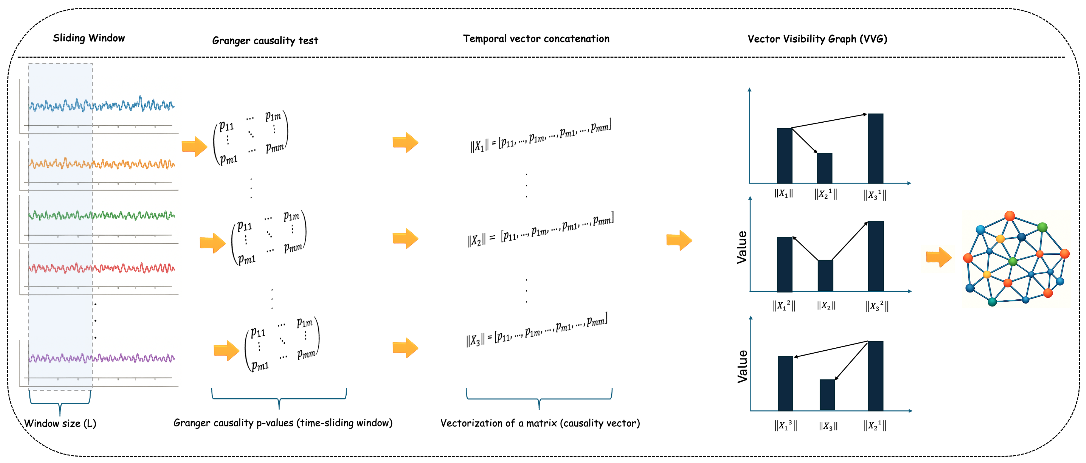
Figure 2.
Synthetic time series for Scenario A. (a) (no coupling). (b) (with coupling); progressive amplitude amplification along the chain. (c) Parameter variation at . (d) Series with abrupt coupling change.
Figure 2.
Synthetic time series for Scenario A. (a) (no coupling). (b) (with coupling); progressive amplitude amplification along the chain. (c) Parameter variation at . (d) Series with abrupt coupling change.
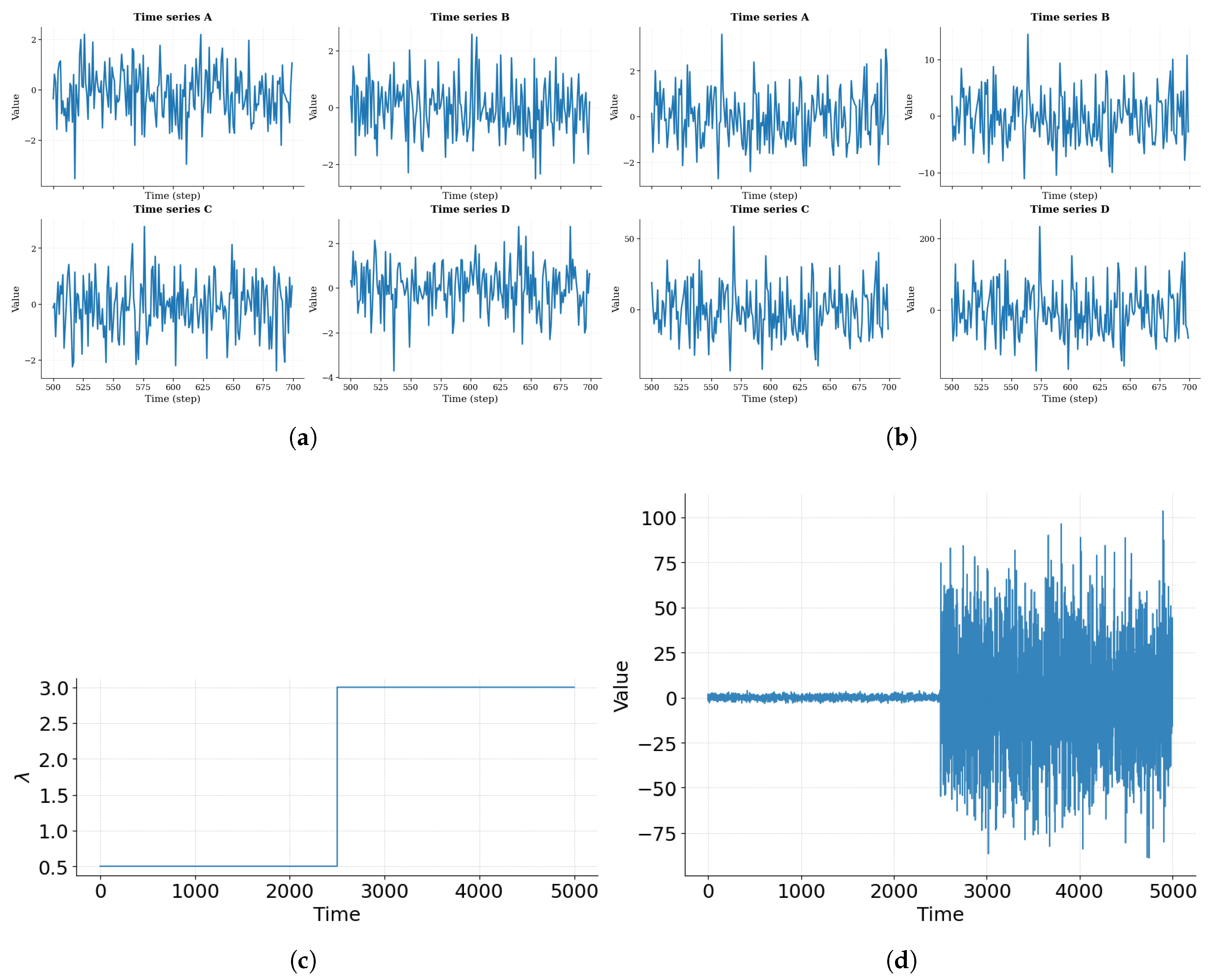
Figure 3.
VVG degree distributions for Scenario A (), comparing (blue) and (orange) under two window sizes. (a) : clear topological separation. (b) : separation lost (low-pass effect).
Figure 3.
VVG degree distributions for Scenario A (), comparing (blue) and (orange) under two window sizes. (a) : clear topological separation. (b) : separation lost (low-pass effect).
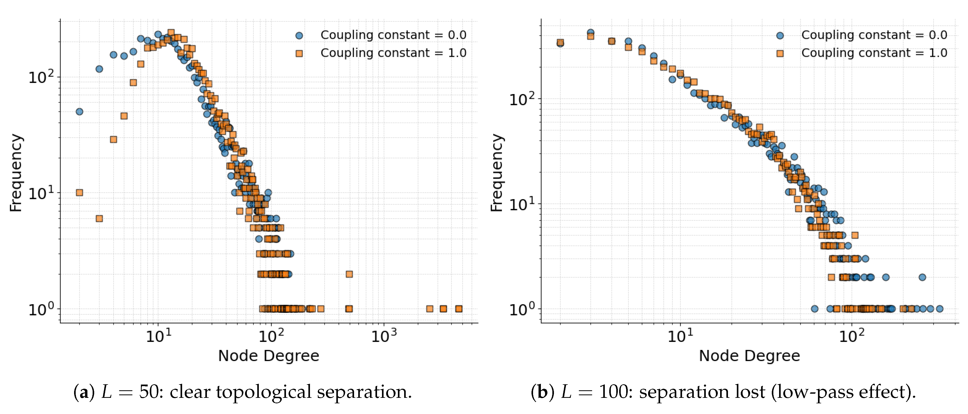
Figure 4.
Degree distributions for series with abrupt coupling change at . (a) , regime change. (b) Comparison with a stochastic series at . (c) : bimodality lost. Bimodality at is the topological signature of the regime transition; it disappears when the window is enlarged.
Figure 4.
Degree distributions for series with abrupt coupling change at . (a) , regime change. (b) Comparison with a stochastic series at . (c) : bimodality lost. Bimodality at is the topological signature of the regime transition; it disappears when the window is enlarged.
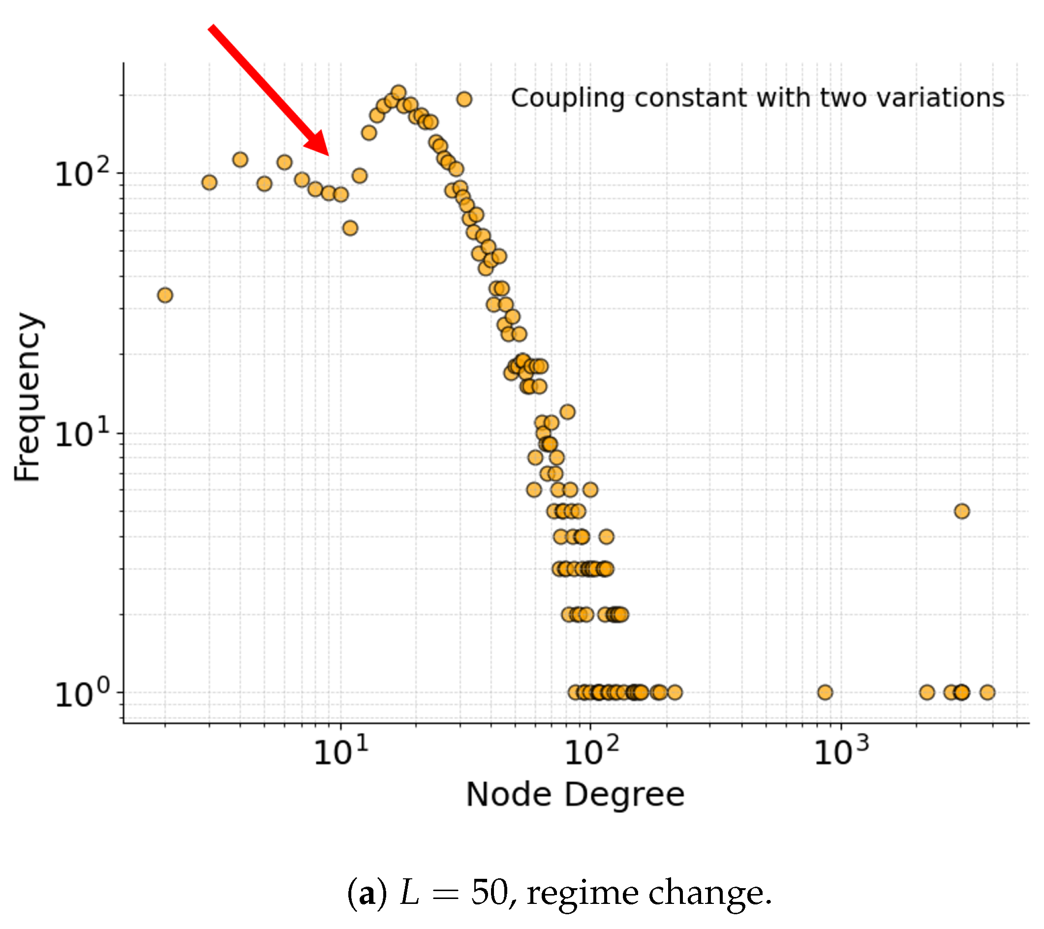
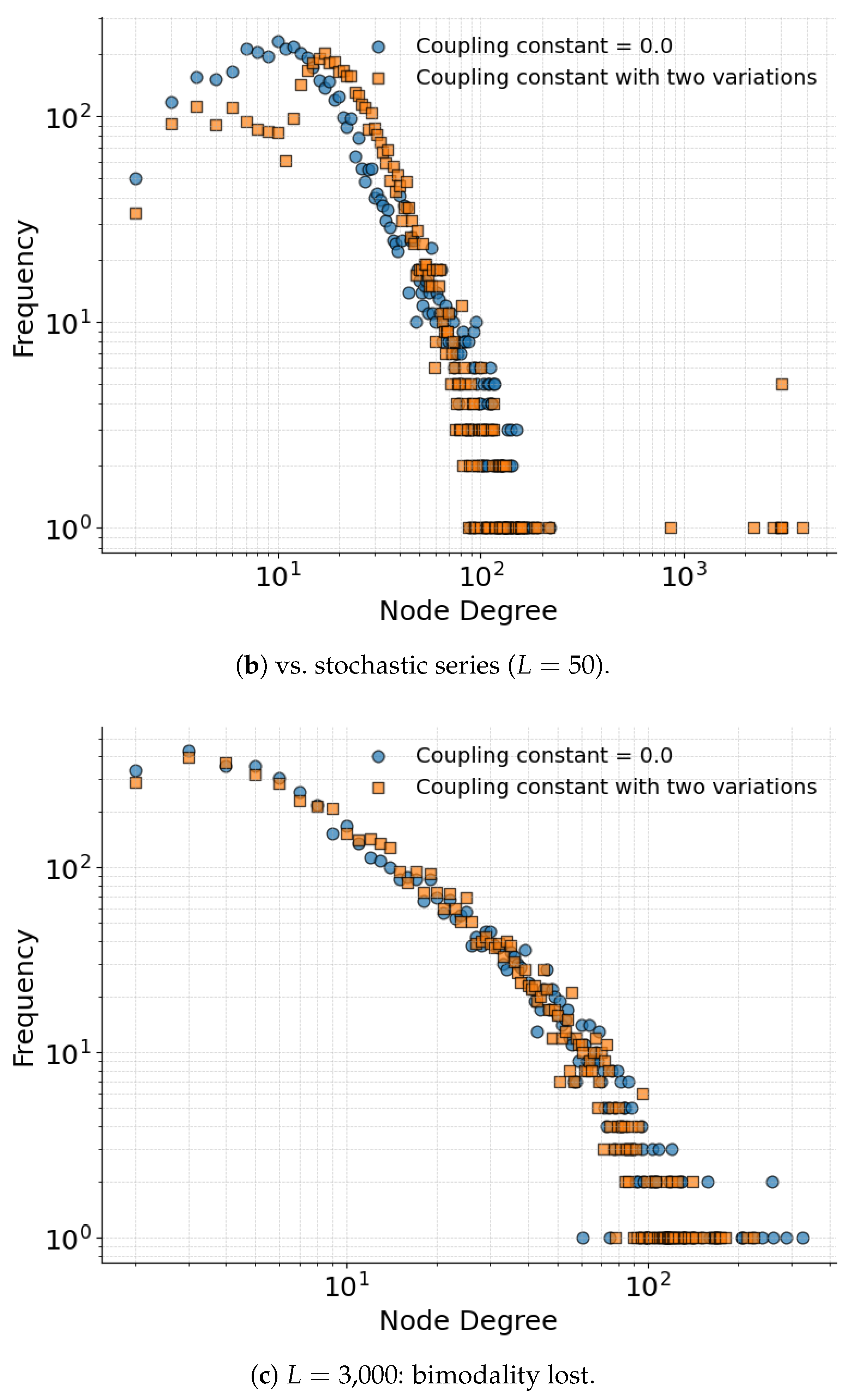
Figure 7.
Normalized mean maximum betweenness centrality as a function of . Dashed curves: fits by Equation (11). Shaded region: 95% confidence band via the delta method. Error bars: standard error over 100 simulations.
Figure 7.
Normalized mean maximum betweenness centrality as a function of . Dashed curves: fits by Equation (11). Shaded region: 95% confidence band via the delta method. Error bars: standard error over 100 simulations.
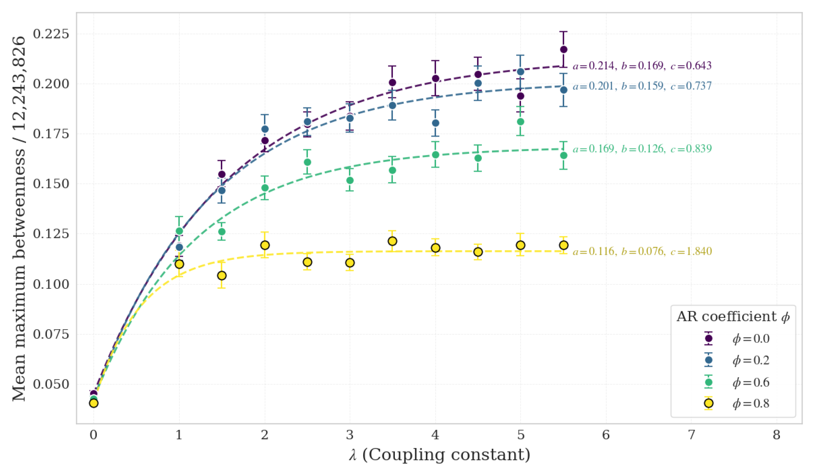
Figure 8.
Row-wise normalized NetLSD heatmaps (Equation (4)) over 100 simulations. Red: topologically distinct graphs; blue: spectrally similar graphs. (a) : sharp boundary at –. (b) : boundary at . (c) : broader band. (d) : leftward shift. The leftward shift of the threshold with increasing is the spectral counterpart of the growth of in the centrality fit.
Figure 8.
Row-wise normalized NetLSD heatmaps (Equation (4)) over 100 simulations. Red: topologically distinct graphs; blue: spectrally similar graphs. (a) : sharp boundary at –. (b) : boundary at . (c) : broader band. (d) : leftward shift. The leftward shift of the threshold with increasing is the spectral counterpart of the growth of in the centrality fit.
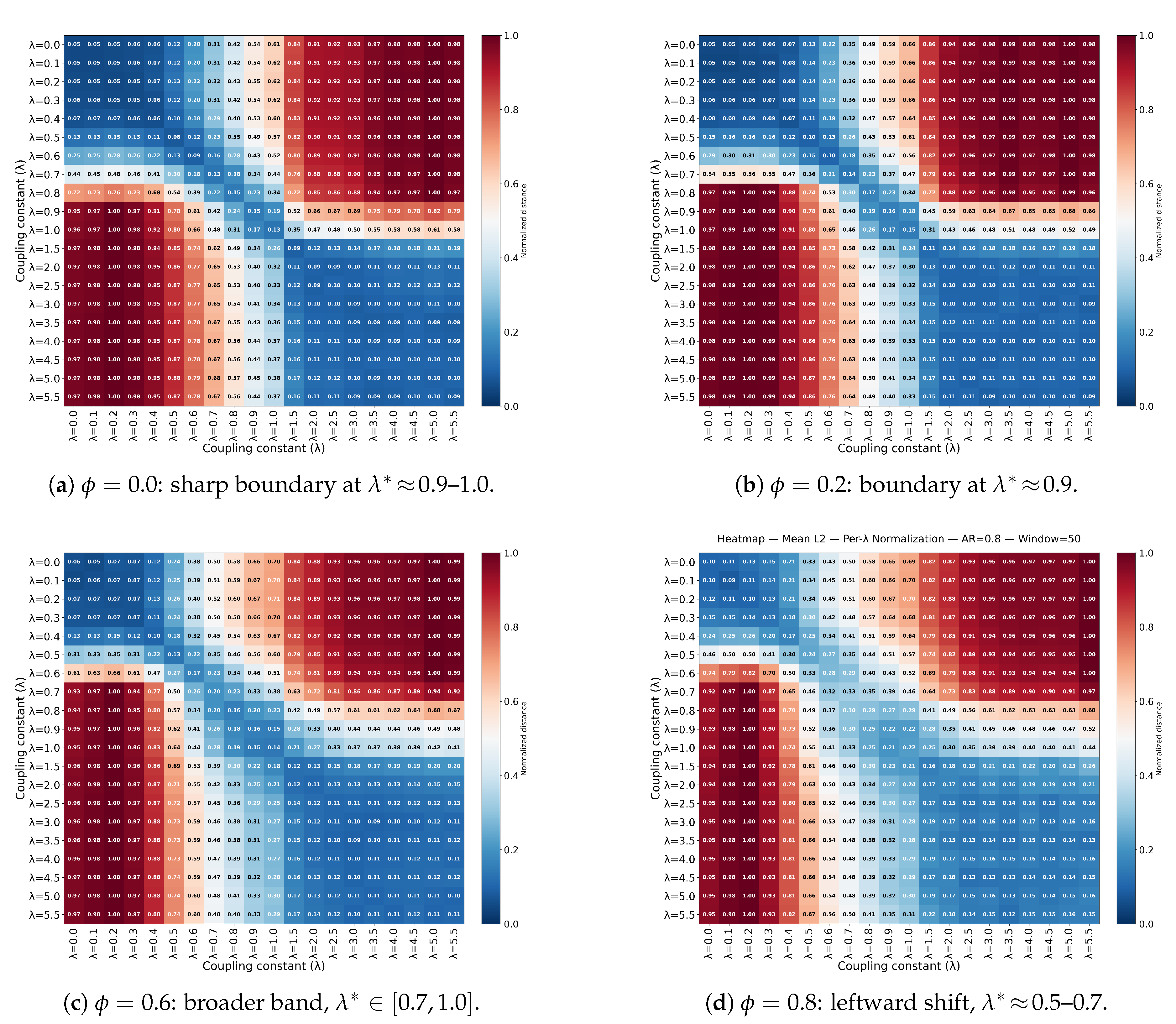
Figure 9.
DTW results for Scenario A as a function of for . (a) Mean transient : U-shaped valley at –; the asterisk marks the only significant point after Holm correction. (b) Number of unique attractors : monotonic collapse with -dependent plateaus (Kruskal–Wallis , ). (c) Largest-basin dominance : sigmoidal transition; diamonds indicate inflection with 95% CI. (d) Plane : quasi-orthogonal organization by (color) and (size).
Figure 9.
DTW results for Scenario A as a function of for . (a) Mean transient : U-shaped valley at –; the asterisk marks the only significant point after Holm correction. (b) Number of unique attractors : monotonic collapse with -dependent plateaus (Kruskal–Wallis , ). (c) Largest-basin dominance : sigmoidal transition; diamonds indicate inflection with 95% CI. (d) Plane : quasi-orthogonal organization by (color) and (size).
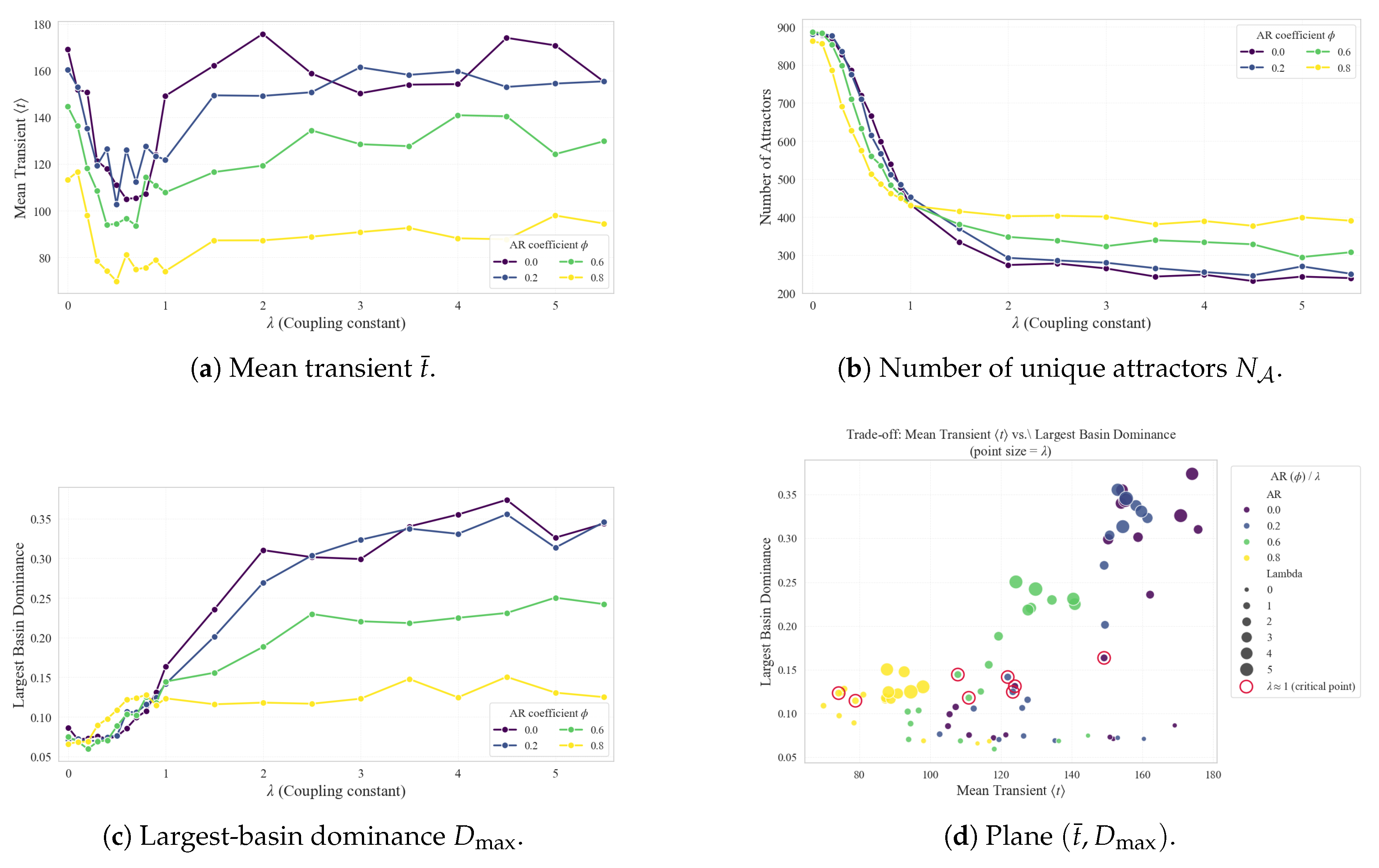
Figure 10.
Top 15 (blue/green) vs. Bottom 15 (orange/red) for Uruguaiana. Three independent metrics show perfect non-parametric separation. (a) Centrality profiles. (b) Mean transient with , . (c) Basin dominance with , .
Figure 10.
Top 15 (blue/green) vs. Bottom 15 (orange/red) for Uruguaiana. Three independent metrics show perfect non-parametric separation. (a) Centrality profiles. (b) Mean transient with , . (c) Basin dominance with , .
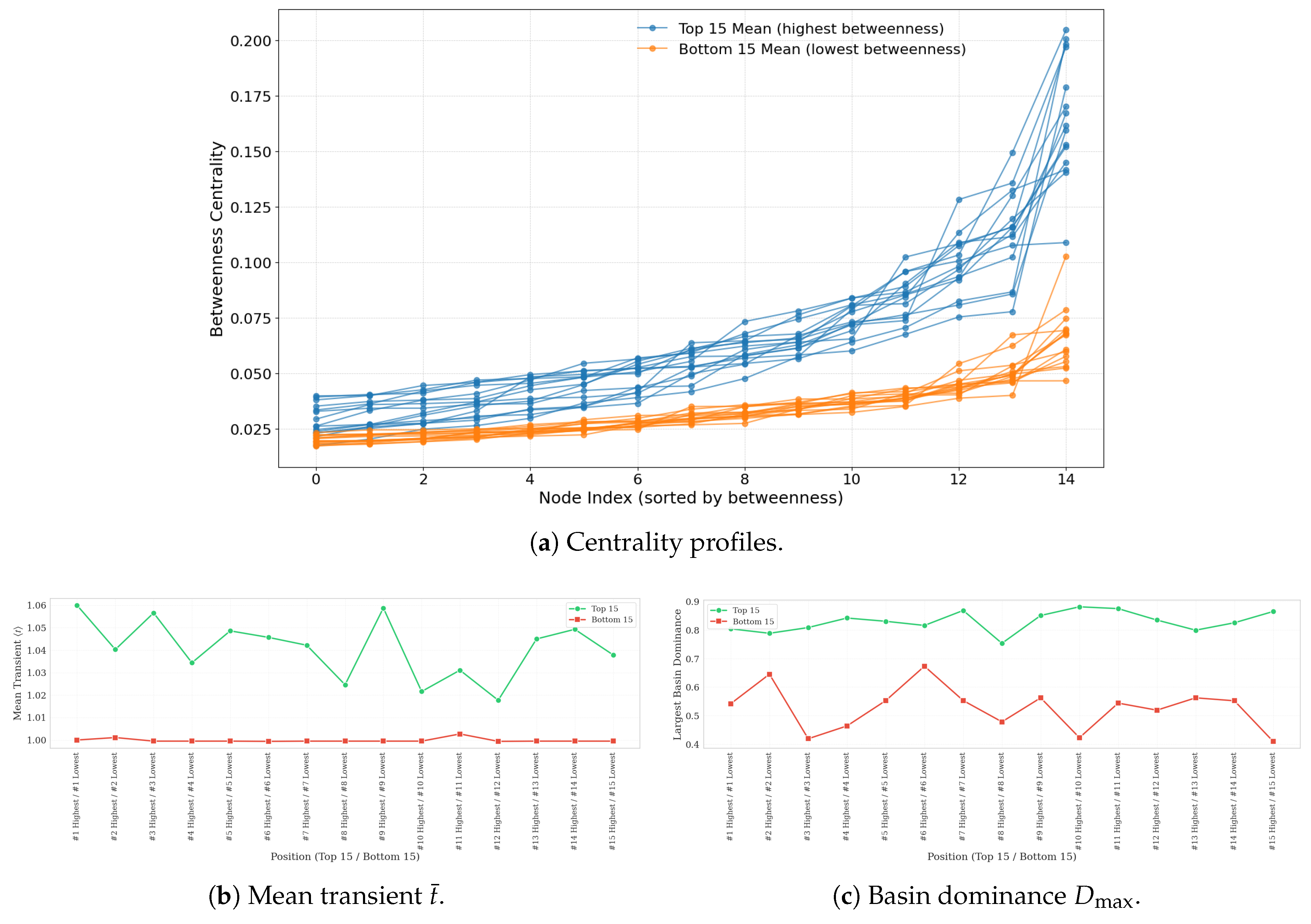

Table 1.
Comparison of methods. Column abbreviations: TV Causal = time-varying causal estimator; VV Graph = vector visibility graph representation; Multimodal Top. = multimodal topological descriptors; Regime Det. = regime-transition detection; Comp. Interp. = compact and interpretable output. Symbol ✓ indicates that the method addresses the corresponding capability; × indicates that it does not; “partial” indicates that the method addresses it only under specific assumptions.
Table 1.
Comparison of methods. Column abbreviations: TV Causal = time-varying causal estimator; VV Graph = vector visibility graph representation; Multimodal Top. = multimodal topological descriptors; Regime Det. = regime-transition detection; Comp. Interp. = compact and interpretable output. Symbol ✓ indicates that the method addresses the corresponding capability; × indicates that it does not; “partial” indicates that the method addresses it only under specific assumptions.
| Method / Work | TV Causal | VV Graph | Multimodal Top. | Regime Det. | Comp. Interp. |
|---|---|---|---|---|---|
| Classical Granger [3] | ✓ | × | × | × | × |
| Transfer Entropy [8] | ✓ | × | × | × | × |
| PCMCI [9] | ✓ | × | × | × | × |
| Classical VG [20] | × | ✓ | × | partial | × |
| Multivariate VVG [13] | × | ✓ | × | × | × |
| Windowed Granger [24] | ✓ | × | × | partial | × |
| Dynamic graph [25] | ✓ | × | × | partial | × |
| NetLSD [16] | × | × | × | × | × |
| This work | ✓ | ✓ | ✓ | ✓ | ✓ |
Table 2.
Saturated exponential fit (Equation (11)): parameters with standard errors, , reduced chi-squared, and AIC comparison against a logistic sigmoid with the same number of parameters ().
Table 2.
Saturated exponential fit (Equation (11)): parameters with standard errors, , reduced chi-squared, and AIC comparison against a logistic sigmoid with the same number of parameters ().
| 0.0 | 0.985 | 0.88 | ||||
| 0.2 | 0.979 | 1.22 | ||||
| 0.6 | 0.960 | 1.70 | ||||
| 0.8 | 0.960 | 0.97 |
Table 3.
Pairwise Mann–Whitney comparisons (Holm correction) for at the plateau (). All pairs significant at .
Table 3.
Pairwise Mann–Whitney comparisons (Holm correction) for at the plateau (). All pairs significant at .
| Sig. | Sig. | ||||||
|---|---|---|---|---|---|---|---|
| 0.0 | 0.2 | ✓ | 0.2 | 0.6 | ✓ | ||
| 0.0 | 0.6 | ✓ | 0.2 | 0.8 | ✓ | ||
| 0.0 | 0.8 | ✓ | 0.6 | 0.8 | ✓ |
Table 4.
Frequency of meteorological variables in Top 15 and Bottom 15 (Uruguaiana). A dash (–) indicates that the variable does not appear in the corresponding group.
Table 4.
Frequency of meteorological variables in Top 15 and Bottom 15 (Uruguaiana). A dash (–) indicates that the variable does not appear in the corresponding group.
| Meteorological Variable | Top 15 | Bottom 15 |
|---|---|---|
| Minimum relative humidity, previous hour (%) | 7 | 3 |
| Maximum atmospheric pressure, previous hour (mB) | 6 | 1 |
| Hourly wind direction (°) | 5 | – |
| Hourly wind speed (m/s) | 5 | – |
| Atmospheric pressure at station level (mB) | 5 | – |
| Hourly relative humidity (%) | 5 | 7 |
| Minimum atmospheric pressure, previous hour (mB) | 4 | – |
| Hourly total precipitation (mm) | 3 | 7 |
| Minimum temperature, previous hour (°C) | – | 7 |
| Maximum temperature, previous hour (°C) | – | 6 |
Disclaimer/Publisher’s Note: The statements, opinions and data contained in all publications are solely those of the individual author(s) and contributor(s) and not of MDPI and/or the editor(s). MDPI and/or the editor(s) disclaim responsibility for any injury to people or property resulting from any ideas, methods, instructions or products referred to in the content. |
© 2026 by the authors. Licensee MDPI, Basel, Switzerland. This article is an open access article distributed under the terms and conditions of the Creative Commons Attribution (CC BY) license (http://creativecommons.org/licenses/by/4.0/).
Copyright: This open access article is published under a Creative Commons CC BY 4.0 license, which permit the free download, distribution, and reuse, provided that the author and preprint are cited in any reuse.


