
Submitted:
27 July 2026
Posted:
28 July 2026
You are already at the latest version
Abstract
Rock cohesion (c ) and angle of internal fricti on (φ ) are core parameters for rock mass stability analysis and engineering design; however, traditional triaxial tests are costly and time-consuming, limiting engineering efficiency.Based on a total of 199 sets of measured data from four rock types (shale, limestone, quartzite, and quartz-mica schist) in the Himalayan region, this study uses P-wave velocity (V_p ), density (ρ ), uniaxial compressive strength (UCS), and tensile strength (TS) as input variables. It employs four models—Support Vector Regression (SVR), Random Forest (RF), multilayer perceptron (MLP), and extreme gradient boosting (XGBoost) to predictc andφ . Hyperparameters were tuned using grid search and Bayesian optimization. We compared unified modeling with rock-type-specific modeling, performed interpretability analysis using SHAP, and tested robustness by introducing Gaussian noise. The results show that XGBoost produced the best predictions atc (test setR^2 = 0.9901, RMSE = 0.512 MPa), while the Bayesian-optimized SVR model yielded the best results atφ (R^2 = 0.9776, RMSE = 0.744°). Rock-type-specific modeling improved theR^2 for limestone atφ by 0.3541; the SHAP contribution for UCS and TS exceeded 70%; Random Forest demonstrated the best noise resistance, with a decrease inR^2 of less than 0.04 under 10% noise. In summary, the strategy proposed in this paper allows for the selection of prediction schemes based on data quality and lithological differences, providing a feasible approach for rapidly obtaining rock strength parameters.
Keywords:
rock mechanics
; cohesion
; angle of internal friction
; machine learning
; lithofacies-based modeling
; SHAP
; robustness
) and angle of internal fricti on ( ) are core parameters for rock mass stability analysis and engineering design; however, traditional triaxial tests are costly and time-consuming, limiting engineering efficiency.Based on a total of 199 sets of measured data from four rock types (shale, limestone, quartzite, and quartz-mica schist) in the Himalayan region, this study uses P-wave velocity ( ), density ( ), uniaxial compressive strength (UCS), and tensile strength (TS) as input variables. It employs four models—Support Vector Regression (SVR), Random Forest (RF), multilayer perceptron (MLP), and extreme gradient boosting (XGBoost) to predict and . Hyperparameters were tuned using grid search and Bayesian optimization. We compared unified modeling with rock-type-specific modeling, performed interpretability analysis using SHAP, and tested robustness by introducing Gaussian noise. The results show that XGBoost produced the best predictions at (test set = 0.9901, RMSE = 0.512 MPa), while the Bayesian-optimized SVR model yielded the best results at ( = 0.9776, RMSE = 0.744°). Rock-type-specific modeling improved the for limestone at by 0.3541; the SHAP contribution for UCS and TS exceeded 70%; Random Forest demonstrated the best noise resistance, with a decrease in of less than 0.04 under 10% noise. In summary, the strategy proposed in this paper allows for the selection of prediction schemes based on data quality and lithological differences, providing a feasible approach for rapidly obtaining rock strength parameters.
1. Introduction
Rock cohesion (c) and angle of internal friction (φ) are two fundamental mechanical parameters describing rock shear strength, widely applied in slope stability analysis, tunnel support design, mining engineering, and foundation bearing capacity evaluation[1,2,3]. Accurately determining these two parameters is crucial for ensuring engineering safety and reducing construction risks. Currently, c and φ are primarily determined through laboratory triaxial compression tests; however, this method suffers from significant issues such as difficult specimen preparation, long testing cycles, high costs, and high variability in results[4]. Therefore, the development of rapid, economical, and reliable indirect prediction methods has become one of the hot topics in rock mechanic’s research.
To overcome these challenges, many researchers have attempted to establish empirical regression relationships between c and φ and easily measurable physical parameters (such as P-wave velocity, density, point load strength, and rebound values)[5,6,7]. For example, Khandelwal and Singh[6] established a linear relationship (R² = 0.96) between wave velocity and uniaxial compressive strength (UCS); Yasar and Erdogan[7] found that wave velocity in carbonate rocks is strongly correlated with density, UCS, and elastic modulus; and Kahraman[5] evaluated the predictive performance of various simple methods for UCS. In addition, Inoue and Ohomi[8], Goktan[9], and Entwisle et al.[10] have also established similar linear or nonlinear regression equations, respectively. However, such empirical formulas are often limited to specific lithologies or regions, and they struggle to capture the complex nonlinear relationships among multiple parameters, resulting in limited generalizability.
In recent years, with the development of artificial intelligence technology, machine learning methods have been introduced into the prediction of rock mechanical parameters.[11,12,13] Compared with traditional regression methods, machine learning can automatically learn the nonlinear mapping between inputs and outputs, handle interactions among high-dimensional features, and possesses strong generalization capabilities. Early studies primarily employed single or simple machine learning models; for example, Kainthola et al.[14] used linear regression and an Adaptive Neuro-Fuzzy Inference System (ANFIS) to establish the relationship between rock strength parameters and P-wave velocity in the Himalayan region, achieving a fitting accuracy of approximately 0.95.Shahani et al.[15] compared Lasso regression, ridge regression, decision trees, and support vector machines (SVM) on the same dataset and found SVM to be the best performer (c’s R² = 0.977). Mahmoodzadeh et al.[16] used Gaussian process regression, SVR, decision trees, and long short-term memory networks (LSTM) to predict strength parameters of intact rocks based on , thereby validating the potential of machine learning methods.
Furthermore, ensemble learning methods have attracted widespread attention due to their advantages in terms of stability and accuracy. Random Forest (RF), as a typical Bagging ensemble model, effectively reduces the risk of overfitting through a voting mechanism involving multiple decision trees and has demonstrated stable performance in rock strength prediction.[17] Khandelwal et al.[18] used a genetic algorithm-optimized artificial neural network (GA-ANN) to predict the cohesion of limestone, achieving a good result of R² = 0.967. Hiba et al.[19] utilized decision trees and random forests to predict c and φ from well logging data, with an average absolute percentage error below 2.4%. Shen and Jimenez[20] applied genetic programming to predict c and φ in sandstone, validating the feasibility of evolutionary algorithms in rock parameter prediction. In recent years, Extreme Gradient Boosting (XGBoost) and its improved versions have achieved leading predictive performance in multiple engineering fields due to their efficient regularization and parallel computing capabilities.[21,22,23,24] Lei et al.[22] proposed the ISSA-XGBoost hybrid model (which optimizes XGBoost using an improved sparrow search algorithm), achieving R² values of 0.982 and 0.932 for the prediction of c and φ, respectively, on the same dataset. Jin et al.[21] and Verma et al.[23] also developed XGBoost frameworks that combine data-driven approaches with interpretability, further enhancing prediction accuracy and model transparency. To clearly illustrate the progress of existing research, Table 1 in summarizes the representative works mentioned above.
Although the aforementioned studies have made positive progress, the following significant gaps remain: (1) Incomplete model comparisons: Most studies use only one or two models, lacking a systematic comparison and fair evaluation of the four representative models—SVR, RF, Multi-Layer Perceptron (MLP), and XGBoost—under identical data conditions.(2) Insufficient optimization of hyperparameters: Model performance is highly dependent on hyperparameter settings, yet many studies use default parameters, failing to fully tap into the models’ potential.(3) Ignoring lithological differences: Different rock types exhibit significant variations in structure, genesis, and mechanical behavior; however, few studies have quantified the impact of “unified modeling” (training models using all lithological data combined) versus “separate modeling by lithology” on prediction accuracy, making it difficult for engineers to determine whether to develop dedicated models for specific rock types.(4) Insufficient interpretability: Machine learning models are often viewed as “black boxes,” and their internal decision-making mechanisms are difficult to understand, limiting engineers’ confidence in the prediction results. Although methods such as SHAP have begun to be applied[25,26,27], systematic analyses in the prediction of rock c and φ remain scarce. (5) Lack of Robustness: In practical engineering applications, input parameters measured in the field (such as wave velocity and density) inevitably contain measurement errors. However, existing studies have scarcely evaluated the models’ tolerance to input noise, leaving the reliability of the models in practical applications uncertain.
To address these shortcomings, this paper builds upon the 199 sets of experimental data for four rock types (shale, limestone, quartzite, and quartz-mica schist) in the Himalayan region published by Kainthola et al.[14] to conduct the following systematic work, with the aim of providing a scientific, systematic, and interpretable solution for the rapid estimation of rock strength parameters:
- Systematic Comparison of Multiple Models and Hyperparameter Optimization: Four representative models—Support Vector Regression (SVR), Random Forest (RF), Multi-Layer Perceptron (MLP), and XGBoost—were selected. Grid search and Bayesian optimization (using the Optuna framework) were employed to tune the hyperparameters of each model, ensuring that all models were compared under optimal conditions, and the performance differences in predicting c and φ were systematically evaluated.
- Quantitative Evaluation of Rock-Type-Specific Modeling Strategies: For the first time on this dataset, we quantitatively compared the predictive performance of unified modeling and rock-type-specific modeling. SVR and RF models were trained independently for each of the four rock types (using the optimal hyperparameters obtained from the unified modeling optimization) and compared with the unified model on the same lithological test subset. The necessity of modeling each rock type separately was quantified using ΔR², revealing the patterns of how lithological differences affect prediction accuracy.
- Model interpretability analysis: The SHAP method was introduced to perform feature importance analysis on the optimal models for the two targets (XGBoost for cohesion c and Bayesian-optimized SVR for internal friction angle φ). Feature importance bar charts, swarm plots, and dependency graphs were generated to reveal the contribution and direction of influence of each input parameter on the prediction results, thereby enhancing the engineering credibility of the models.
- Robustness Evaluation and Engineering Applications: For the first time, multi-model robustness comparison tests were conducted on this dataset. Gaussian noise at different levels (0%, 1%, 3%, 5%, 10%) was added to the input features (
, density, UCS, UTS) in the test set to simulate field measurement errors. The best versions of each of the four models, obtained through hyperparameter optimization, were used in the comparison. The decline in R² for each model under different noise levels was evaluated to identify the model least sensitive to noise, thereby providing a basis for model selection under conditions of uncertain field data quality. Furthermore, by synthesizing all analytical results, this study proposes model selection guidelines and engineering application recommendations for field engineers.
Through the systematic comparison and in-depth analysis described above, this paper aims to provide a scientific, systematic, and interpretable machine learning solution for the rapid estimation of rock strength parameters, and to offer clear guidance for field engineers in selecting appropriate prediction models under varying data quality conditions.
2. Data and Methods
2.1. Data Sources and Sample Characteristics
The data used in this study were obtained from the physical and mechanical test results of four rock types (shale, limestone, quartzite, and quartz-mica schist) collected by Kainthola et al.[14] in the Luhri region of the Himalayas. Following the methods recommended by the ISRM, uniaxial compression, Brazilian split, triaxial compression, and P-wave velocity tests were conducted, yielding a total of 199 valid sample sets. Each sample set includes six parameters: P-wave velocity (m/s), density (g/cm³), uniaxial compressive strength (MPa), tensile strength (MPa), cohesion (MPa), and angle of internal friction (°).
The sample sizes and statistical characteristics (meaning ± standard deviation) for each rock type are listed in Table 2 at. As shown2 at quartzite had the highest average UCS (198.53 MPa), while quartz-mica schist had the lowest (58.15 MPa), covering a wide range from soft to hard rocks; The mean cohesion of slate is 19.13 MPa, that of limestone is 18.99 MPa, that of quartzite is 25.80 MPa, and that of quartz-mica schist is 13.14 MPa; the mean angle of internal friction ranges from 31.53° to 35.95°. The data distribution is reasonable, with no obvious outliers.
1Note: The values in the table represent “mean ± standard deviation”; n denotes the sample size.
To further reveal the intrinsic relationships among the parameters, Figure 1 shows the Pearson correlation coefficient matrix for input and output parameters. As shown in Figure1 , the uniaxial compressive strength (UCS) exhibits a strong positive correlation with cohesion (c) (r ≈ 0.94) and a significant positive correlation with the angle of internal friction (φ) (r ≈ 0.72); the correlation coefficients between tensile strength (TS) and c and φ are 0.89 and 0.68, respectively; there is a moderate correlation between P-wave velocity () and density (ρ) (r ≈ 0.65), but the correlation with the output parameters is relatively weak. These analysis results further validate the rationale for selecting UCS and TS as core input features.
Figure 2 illustrates the overall technical workflow of this study. First, the raw data was Z-score standardized and split into training and testing sets in a 70%/30% ratio; model selection was performed using 5-fold cross-validation; Subsequently, four models—SVR, RF, MLP, and XGBoost—are trained separately, with hyperparameter tuning performed via grid search and Bayesian optimization; based on this, comparative lithofacies modeling (quantified by ΔR²), SHAP interpretability analysis, and robustness testing are conducted; finally, the performance of each model is comprehensively evaluated, and the optimal model is recommended.
2.2. Data Preprocessing
To eliminate the influence of units, the input features were Z-score normalized: , where and represent the mean and standard deviation of each feature in the training set, respectively. All 199 samples were randomly split into a 70% training set and a 30% test set (random seed 42), resulting in a training set of 139 samples and a test set of 60 samples. During the hyperparameter optimization process, 5-fold cross-validation was used, applied only to the training set.
2.3. Machine Learning Models
This study selected four representative regression models: Support Vector Regression (SVR), Random Forest (RF), Multi-Layer Perceptron (MLP), and XGBoost. The principles, objective functions, and key hyperparameters of each model are described below.
2.3.1. Support Vector Regression (SVR)
SVR is based on statistical learning theory and uses a kernel function to map input data to a high-dimensional feature space, thereby constructing an optimal linear regression function[28]. It employs a -insensitive loss function, which penalizes only those samples where the deviation between the predicted and true values exceeds . Its optimization objective is given in Equation (1):
Subject to the constraints in Equation (2):
where represents the kernel mapping (this paper uses the RBF kernel), is the penalty coefficient, and controls the width of the insensitivity band. The main hyperparameters include , kernel parameters , and .
2.3.2. Random Forest (RF)
RF is a representative algorithm of Bagging ensemble learning, which reduces the risk of overfitting by constructing multiple independent decision trees and taking their average[17]. For regression tasks, the final predicted value is the arithmetic mean of the predicted values from all trees, as given in Equation (3):
where is the number of trees, and is the predicted value of the th tree. Each tree is generated based on Bootstrap sampling and a random subset of features. Key hyperparameters include the number of trees , maximum depth , the minimum number of samples required for node splitting , and the minimum number of samples at leaf nodes .
2.3.3. Multi-Layer Perceptron (MLP)
An MLP is a feedforward artificial neural network[29,30] consisting of an input layer, hidden layers, and an output layer. This paper adopts an MLP architecture with two hidden layers (containing 64 and 32 neurons, respectively), where the activation function for the hidden layers is the rectified linear unit (ReLU), defined in Equation (4):
The output layer uses a linear activation function, which is suitable for regression tasks. The network is trained by minimizing the mean squared error (MSE) loss, as shown in Equation (5):
The Adam optimizer is used, and L2 regularization (parameter ` `) and an early stopping strategy are introduced to prevent overfitting. Key hyperparameters include the hidden layer structure, the regularization coefficient ` `, and the initial learning rate ` `.
2.3.4. Extreme Gradient Boosting (XGBoost)
XGBoost is an efficient implementation of gradient-boosted decision trees[22] that fits residuals by iteratively adding regression trees. At step , the objective function is defined in Equation (6):
where is the loss function (MSE in this paper), and is the regularization term (Equation (7)):
Here, is the number of leaf nodes in the tree, is the weight of the leaf nodes, and and are the regularization coefficients. XGBoost uses second-order gradient information to accelerate convergence and has built-in parallel computing capabilities. The main hyperparameters include the learning rate , tree depth , number of trees , subsampling ratio , and feature sampling ratio .
All models were implemented using the Scikit-learn [^1] and XGBoost [^2] libraries.
2.4. Hyperparameter Optimization
Two strategies were used for hyperparameter optimization, with the average score from 5-fold cross-validation ( ) serving as the evaluation metric.
Grid Search: The candidate hyperparameter values for each model are listed in Table 3 at. All combinations were iterated through selecting the optimal parameters.
Bayesian Optimization: To further improve performance, the Optuna framework (TPE sampler) was used to search within a broader continuous space; the search ranges for each model are shown in Table 4 at. With the goal of minimizing cross-validation1-R^2 , 100 trials were conducted for each model, and a median pruning strategy was employed to accelerate the process. The optimal model for each target was ultimately selected based on test set performance (results are shown in Table 5 at; see Section 3). The two hyperparameter optimization strategies described above were applied only to the unified dataset (all lithologies combined); the resulting optimal hyperparameters will be used for subsequent unified modeling as well as lithology-specific modeling (see Section 2.5).
2.5. Lithology-Specific Modeling Strategies
To quantify the impact of lithological differences on prediction accuracy, this paper compares the performance of unified modeling (training on the entire dataset) with lithology-specific modeling (training each rock type separately).For rock-type-specific modeling, the optimal hyperparameters obtained from unified modeling via hyperparameter optimization (grid search or Bayesian optimization) were directly applied to retrain the SVR and RF models on subsets of shale, limestone, quartzite, and quartz-mica schist, respectively, without conducting independent hyperparameter searches for each rock-type subset. This ensures a fair comparison, as only the lithological composition of the training data is altered, while the model architecture and hyperparameters remain consistent. The trained lithology-specific models are applied to the corresponding test subsets for each rock type, and the coefficient of determination ( ) is calculated and compared with the coefficient of determination ( ) of the unified model on the same test subsets. We define ; if is positive and has a large absolute value, it indicates that modeling specifically for that lithology can significantly improve prediction accuracy.
2.6. Model Interpretability: SHAP Analysis
The SHAP (SHapley Additive exPlanations) method[27] was used to interpret the optimal model. For tree-based models (XGBoost, RF), Tree Explainer was employed to generate feature importance bar charts, swarm plots, and dependency graphs, thereby analyzing the contribution and direction of influence of each input feature.
2.7. Robustness Analysis
To simulate field measurement errors, Gaussian noise at different levels was added to the input features of the test set, as shown in Equation (8):
where is the standard deviation of each feature in the training set, and the noise levels are set to 0, 0.01, 0.03, 0.05, and 0.10 (corresponding to 0%–10%). With a fixed random seed of 42, we calculated the for each model at different noise levels, plotted performance degradation curves, and compared the models’ tolerance to input errors. In the robustness analysis, the four models (SVR, RF, MLP, and XGBoost) were all compared using their best versions, optimized with their respective hyperparameters.
2.8. Evaluation Metrics
The determination coefficient , mean absolute error (MAE), and root mean square error (RMSE) were used to evaluate the models’ predictive performance on the test set, calculated using Equations (9):
where is the true value, is the predicted value, and is the meaning of the true values.
[^1]: Pedregosa F, et al. Scikit-learn: Machine learning in Python. Journal of Machine Learning Research, 2011, 12: 2825-2830.
[^2]: Chen T, Guestrin C. XGBoost: A scalable tree boosting system. In: Proceedings of the 22nd ACM SIGKDD, 2016: 785–794.
3. Results
3.1. Model Performance Comparison
The prediction performance of each model on the test set, obtained through grid search and Bayesian optimization, is summarized in Table 5 at. For cohesive strength , XGBoost achieved the highest accuracy under grid search ( , RMSE = 0.512 MPa), and Bayesian optimization failed to further improve this result; Random Forest (RF) also achieved similar results ( ).For the internal friction angle , Bayesian optimization significantly improved the predictive capability of Support Vector Regression (SVR), increasing the accuracy from 0.9176 in grid search to 0.9776, and reducing the RMSE from 1.426° to 0.744°.At the same time, the Multi-Layer Perceptron (MLP) showed marked improvement in predicting under Bayesian optimization ( , rising from 0.9504 to 0.9787).The above results indicate that Bayesian optimization possesses stronger exploration capabilities in continuous, high-dimensional parameter spaces and is particularly suitable for models sensitive to hyperparameters, such as kernel methods (SVR) and neural networks (MLP). For tree-based models (RF and XGBoost), grid search is sufficient to achieve near-optimal performance.
* Note: Bold text indicates the best performance on that target.
Figure 3 illustrates the convergence of the MLP and XGBoost models during training. The MLP’s loss curve decreases rapidly during the first 200 iterations and enters a plateau after approximately 500 iterations, indicating that the network has fully converged. XGBoost’s validation RMSE continued to decrease as the number of trees increased, entering a plateau after approximately 450 trees. Subsequently, the validation error stabilized, and the early stopping mechanism automatically terminated training at this point, effectively preventing overfitting. Both convergence curves validate the stability of the model training process and the rationality of the hyperparameter selection.
Figure 4 shows scatter plots of the predicted and actual values for the four models on the test set (using the finally selected model as an example). The points in all subplots are closely clustered around the 45° reference line, with those for XGBoost (c) and SVR (φ) being the most concentrated, consistent with the higher values in Table 5 at.
3.2. Comparison of Modeling by Rock Type
To further evaluate the impact of lithological differences on prediction accuracy, this study used the optimal hyperparameters obtained from unified modeling optimization to independently train SVR and RF models on subsets of shale, limestone, quartzite, and quartz-mica schist, and evaluated them on corresponding lithological test subsets. The prediction performance of the unified model on the same test subset served as the benchmark for comparison. Table 6 in REF _Ref234937826 \h lists the and the difference between the lithology-specific models and the unified model.
Values and Differences Between Lithological and Unified Modeling.
The results show that:
- Quartzite and quartz-mica schist: The absolute values of
for all models are less than 0.01; lithofacies-specific modeling provides almost no improvement, and the unified model is sufficient.
- Slate: Rock-type-specific RF and SVR models significantly improved predictions of the internal friction angle (
) ( , reaching +0.1410 and +0.0864, respectively), but did not significantly improve predictions of cohesion ( ) (RF was +0.0418, while SVR showed a slight decrease). This indicates that the mechanical behavior of slate is complex, and separate modeling is more valuable for .
- Limestone: Lithological modeling significantly improves the prediction of the internal friction angle (
), particularly with SVR, which achieves a of +0.3541 (rising from 0.5954 to 0.9495); RF also improves the by 0.0994. There is also some improvement in the prediction of the (SVR +0.0627). Limestone is a chemical sedimentary rock with a relatively uniform structure; therefore, targeted modeling can significantly improve prediction accuracy.
The bar chart in Figure 5 visually illustrates the comparison results between the “ “ models mentioned above.
3.3. SHAP Explainability Analysis
To further reveal the internal mechanisms of model predictions and identify key input features, the SHAP (SHapley Additive exPlanations) method[27] was used to interpret the two optimal models: cohesion used XGBoost (optimized via grid search), and internal friction angle used SVR (optimized via Bayesian optimization). Based on game theory, SHAP provides both global and local explanations by calculating the marginal contribution of each feature to the prediction result.
Figure 6 (a) shows the feature importance bar chart (average absolute SHAP values) for the XGBoost model’s prediction of . It can be seen that uniaxial compressive strength ( ) makes the largest contribution, with an average SHAP value of approximately 1.2; tensile strength ( ) follows (approximately 0.6); while the contributions of P-wave velocity ( ) and density ( ) are both less than 0.2. This indicates that and are the most critical mechanical parameters for predicting cohesion. The swarm plots in Figure 6 (b) illustrate the direction of influence for each feature: and —the larger the value (red points), the stronger the positive contribution to the predicted value (positive SHAP value); and have a smaller influence, and some samples show a negative correlation. This result is consistent with the fundamental laws of rock mechanics—the higher the rock strength, the greater its cohesion typically is. Figure 6 (c) shows the dependency plot for , indicating that the SHAP value increases monotonically as increases, further validating its core driving role.
Figure 6 (d–f) present the SHAP analysis results of SVR predictions for . The feature importance bar charts ( Figure 6 d) show that and remain the most significant features, but the relative importance of density ( ) has increased, while wave velocity ( ) contributes the least. The swarm plots (Figure 6 e) indicate that and also have a positive influence on , while the direction of influence for is inconsistent, which may be related to differences in mineral composition among different rock types. The dependency plot for (Figure 6 f) again shows a monotonically increasing trend, confirming its significant positive effect on the internal friction angle.
In summary, the SHAP analysis clearly reveals that and are the dominant features for predicting and , with their combined SHAP contribution exceeding 70%; the model’s predictions align with physical intuition. In engineering practice, priority should be given to accurately measuring these two strength indices; wave velocity and density can serve as auxiliary parameters and may be appropriately simplified when data collection is limited.
); (b) XGBoost swarm plot ( ); (c) XGBoost dependency graph ( , ); (d) SVR feature importance ( ); (e) SVR swarm plot ( ); (f) SVR dependency graph ( , ).
3.4. Robustness Analysis
In practical engineering applications, on-site measurements of rock physical and mechanical parameters inevitably contain errors. To simulate this uncertainty and evaluate the tolerance of each model to input noise, this paper adds Gaussian noise at different levels to the features in the test set ( , , , ): , corresponding to relative noise intensities of 0%, 1%, 3%, 5%, and 10% (based on the standard deviation of each feature in the training set). To eliminate random fluctuations, each noise level was repeated 5 times and averaged . Figure 7 shows the performance degradation curves of four models (SVR, RF, MLP, XGBoost) at different noise levels; each model was compared using its best version optimized with hyperparameters.
Cohesion (Figure 7 a): XGBoost achieves the highest accuracy in the absence of noise ( ) but is the most sensitive to noise; under 10% noise, drops by 0.0244 to 0.9657.SVR shows the smallest decline (0.0034, from 0.9835 to 0.9801) and demonstrates the best robustness; MLP (decrease of 0.0077) and RF (decrease of 0.0135) fall in the middle. It is worth noting that while SVR has lower accuracy than XGBoost and RF in the absence of noise, it exhibits the strongest resistance to noise.
(Figure 7 b): MLP showed the smallest decrease (0.0236, from 0.9199 to 0.8963), while RF and XGBoost fell in the middle (decreases of 0.0358 and 0.0337, respectively). SVR showed the most significant decline (0.1216, dropping sharply from 0.9776 to 0.8560), even though it achieved the highest accuracy in the absence of noise. This difference may stem from the models’ mechanisms: as a kernel method, SVR’s decision boundary depends on all support vectors, making it susceptible to input noise that can disrupt the global optimization structure; in contrast, tree-based models (RF, XGBoost) make decisions based on feature splitting thresholds and are inherently resistant to noise.
The above results indicate that no single model is optimal across all metrics: XGBoost leads in accuracy without noise but has weaker robustness; SVR achieves extremely high accuracy in predicting but is sensitive to noise; RF strikes the best balance between accuracy and robustness (c: , with a decline of only 0.0135 under 10% noise; : , with a decline of 0.0358). All things considered, Random Forest (RF) is the most suitable model for field applications—when data quality is high, XGBoost (c) or SVR ( ) can be selected to achieve peak accuracy; when data contains significant uncertainty, RF is the more reliable choice.
; (b) Internal friction angle The above analyses of accuracy, robustness, and feature importance provide a quantitative basis for model selection in engineering applications; Section 4.6 will present systematic engineering application guidelines based on these findings.
4. Discussion and Recommendations for Engineering Applications
This study systematically compared the performance of four machine learning models (SVR, RF, MLP, and XGBoost) in predicting rock cohesion and internal friction angle , and comprehensively evaluated the models through hyperparameter optimization, rock-type-specific modeling, SHAP explainability analysis, and robustness testing. The following discussion focuses on several key aspects.
4.1. Comparison of Model Performance with Previous Studies
Compared with previous studies, the accuracy of the model in this paper has been significantly improved. Kainthola et al.[14] achieved an accuracy of approximately using linear regression and ANFIS on the same dataset; Shahani et al.[15] obtained for and for using SVM; the ISSA-XGBoost model proposed by Lei et al.[22] achieved for and , with values of 0.982 and 0.932, respectively.After hyperparameter optimization in this study, XGBoost achieved a prediction accuracy of for , while SVR (Bayesian optimization) achieved for —both outperforming the aforementioned results. This is primarily attributed to: (1) systematic hyperparameter optimization (grid search + Bayesian optimization); (2) multi-model comparison to select the most suitable model for each objective; and (3) the fine-tuning of SVR hyperparameters via Bayesian optimization, which significantly improved the prediction accuracy for .
4.2. Engineering Significance of Rock-Type-Specific Modeling
The results of lithofacies-specific modeling (Table 6 ) indicate that the impact of lithofacies differences on prediction accuracy cannot be ignored. In the prediction of limestone ( ), the lithofacies-specific SVR achieved a as high as +0.3541, while the RF for slate reached +0.1410; in contrast, the for quartzite and quartz-mica schist were both less than 0.01.This difference can be explained from the perspectives of rock genesis and structure: limestone is a chemical sedimentary rock with a relatively uniform structure and more predictable mechanical behavior; slate is a metamorphic rock with a foliated structure and complex mechanical behavior, but modeling it separately can still improve the prediction of ;Since quartzite and quartz-mica schist have relatively stable mineral compositions and structures, a unified model is sufficient. Therefore, in practical engineering applications, if the subject of study consists primarily of limestone, it is recommended to develop a dedicated prediction model; if multiple rock types are involved but quartzite-type rocks predominate, a unified model can meet the requirements.
4.3. Practical Value of Model Interpretability and Robustness
SHAP analysis (Figure 6) clearly reveals that and are the most critical features for predicting and . This is consistent with the fundamental theory of rock mechanics—rock strength indices directly determine its shear resistance. This finding provides field engineers with a basis for feature selection: when data collection is limited, priority should be given to ensuring the measurement accuracy of and , while and can serve as auxiliary parameters.
Robustness analysis (Figure 7) shows that RF achieves the optimal balance between accuracy and noise resistance, while XGBoost and SVR, although more accurate in the absence of noise, are more sensitive to input noise. This suggests that in practical engineering applications, model selection should be based on a trade-off considering data quality: if field test conditions are favorable (noise < 3%), XGBoost (c) or SVR ( ) can be selected to achieve the highest accuracy; if the data contains significant uncertainty, RF is the more prudent choice.
4.4. Trade-off Between Accuracy and Robustness
This study reveals an important phenomenon: high-accuracy models often come at the expense of robustness. XGBoost achieved the highest prediction accuracy for (0.9901), but its dropped by 0.0244 under 10% noise; SVR achieved the highest prediction accuracy for (0.9776), but its dropped by as much as 0.1216. This may be because these two models are overly sensitive to subtle patterns in the training data, and noise tends to amplify their prediction biases. In contrast, the Bagging ensemble strategy of RF effectively reduces variance by averaging the predictions of multiple trees, thereby achieving stronger noise resistance. This finding provides direct guidance for engineering applications: when data quality is controllable, one should pursue maximum accuracy; when data quality is uncertain, model stability should be prioritized.
4.5. Limitations and Future Work
This study has the following limitations: (1) The dataset is small (199 samples) and consists entirely of data from the Himalayan region; the model’s generalization ability needs to be validated under other geological conditions; (2) Input features are limited to laboratory test parameters and do not consider in-situ field test data (such as RQD and joint characteristics); (3) The study does not account for the influence of engineering factors—such as moisture content and weathering degree—on and .Future work could be expanded in the following directions: (1) Collect data from multiple mining areas and rock types to construct a more generalizable model; (2) Introduce field test parameters (such as rebound values and borehole data) as supplementary inputs; (3) Explore deep learning methods (such as Transformers) or ensemble strategies (Stacking) to further improve prediction performance; (4) Develop a simple, web-based prediction tool for easy application at engineering sites.
4.6. Recommendations for Engineering Applications
Based on the systematic comparison and comprehensive evaluation described above, this section offers specific recommendations from an engineering practicality perspective regarding model selection, feature extraction, and modeling strategies for rock strength parameter prediction, with the aim of providing actionable guidance for field engineers.
For quick reference, Table 7 summarizes the recommended approaches under different engineering conditions.
- Model Selection Recommendations: Field engineers should select models based on data quality: When data quality is high (
, density, UCS, and UTS obtained from standard indoor tests), XGBoost is recommended for predicting cohesion (R² = 0.9901, RMSE = 0.512 MPa), and SVR (Bayesian optimization) is recommended for predicting the angle of internal friction (R² = 0.9776, RMSE = 0.744°);When data contain measurement errors or only partial parameters are available, Random Forest (RF) is recommended, as it maintains high accuracy while offering the strongest resistance to noise, with the smallest decrease in R² under 10% noise (c: 0.0034, φ: 0.0358). If both c and φ need to be predicted simultaneously with balanced accuracy requirements, RF is the most reliable choice.
- Feature Selection Priority: SHAP analysis (Figure 6) indicates that UCS and UTS are the most significant features influencing c and φ, with their combined contribution exceeding 70%. When field data collection is limited, priority should be given to ensuring the measurement accuracy of UCS and UTS;
and density can serve as auxiliary parameters and be measured supplementarily when conditions permit. If only UCS and UTS are available, satisfactory prediction results can still be achieved; if only and density are available, the accuracy of predicting the internal friction angle is acceptable (SVR φ: R² ≈ 0.93), but the accuracy of predicting cohesion will decrease significantly.
- 3.
- Rock-Type-Specific Modeling Strategy: For limestone-type rocks, it is recommended to establish separate prediction models—the R² of rock-type-specific SVR for φ increases from 0.5954 in the unified model to 0.9495 (ΔR² = 0.3541), representing a 59.5% improvement; For shale-type rocks, it is recommended to model the internal friction angle separately (RF lithology-specific ΔR² = 0.1410); for quartzite and quartz-mica schist, the unified model is sufficient (ΔR² < 0.01).
- 4.
- Field Application Process: Field engineers are advised to follow these steps: (a) Assess the types of available input parameters and the accuracy of testing to determine the data quality grade; (b) Identify rock types and determine whether rock-type-specific modeling is required; (c) Select an appropriate model based on the prediction target (c or φ) and Table 7;(d) Input the standardized parameters to perform predictions; (e) Use the prediction results as a reference for preliminary design or feasibility studies; however, critical engineering components still require verification through laboratory testing.
The above recommendations are based on the specific dataset and modeling conditions described in this paper; appropriate adjustments should be made in actual engineering applications based on specific circumstances.
5. Conclusions
Based on 199 data sets from four rock types in the Himalayan region, this study employed four machine learning models—SVR, RF, MLP, and XGBoost—to predict cohesion and internal friction angle . Through hyperparameter optimization, rock-type-specific modeling, SHAP interpretability analysis, and robustness testing, the following main conclusions were drawn:
- Hyperparameter optimization significantly improved model performance: XGBoost (grid search) achieved a
and an RMSE of 0.512 MPa for predictions of ; SVR (Bayesian optimization) achieved a and an RMSE of 0.744° for predictions of , both outperforming previous studies. Bayesian optimization particularly improved the MLP’s predictions for ( , increasing from 0.9504 to 0.9787).
- Lithofacies-specific modeling is crucial for specific rock types: in the prediction of
for limestone, the lithofacies-specific SVR’s reached as high as +0.3541, while the RF for shale also reached +0.1410. It is recommended to model rocks with uniform structures, such as limestone, separately; for shale, selective separate modeling can be performed based on the prediction target (φ); and for rocks such as quartzite, a unified model is sufficient.
- SHAP analysis revealed the key controlling factors:
and are the most significant features for predicting and , contributing over 70% of the variance. In engineering practice, priority should be given to accurately measuring these two strength indices.
There are significant differences in model robustness: XGBoost and SVR achieve the highest accuracy in the absence of noise but are sensitive to noise; RF strikes the best balance between accuracy (c: 0.9891, φ: 0.9453) and robustness (a decrease in of less than 0.04 under 10% noise), making it the most suitable model for field applications.
Model selection should balance accuracy and robustness: When data quality is high, XGBoost (c) or SVR ( ) can be selected to achieve maximum accuracy; when data uncertainty exists, RF is the more prudent choice.
Recommendations for Engineering Applications: Based on data quality, lithological conditions, and prediction objectives, this paper provides a systematic model selection guide (Table 7). Field engineers are advised to follow a five-step process: “Data Quality Assessment → Lithological Identification → Objective Definition → Model Selection → Prediction Validation”; Random Forest (RF) is the most suitable model for field applications; when data quality is high, XGBoost (c) or SVR (φ) can be used to achieve maximum accuracy; for limestone and shale, it is recommended to model by lithology, while a unified model can be used for quartzite-type rocks. Prediction results can be used as a reference for preliminary design, but critical engineering decisions still require verification through laboratory testing.
Author Contributions
Conceptualization, J.X. and X.X.; methodology, J.X. and X.X.; software, J.X.; validation, J.X., X.X.; formal analysis, J.X.; investigation, J.X.; resources, J.X. and X.X.; data curation, J.X.; writing—original draft preparation, J.X.; writing—review and editing, X.X.; visualization, J.X.; supervision, X.X.; project administration, J.X. All authors have read and agreed to the published version of the manuscript.
Funding
This research received no external funding.
Institutional Review Board Statement
Not applicable.
Informed Consent Statement
Not applicable.
Data Availability Statement
The data that support the findings of this study are available from the corresponding author upon reasonable request.
Conflicts of Interest
The authors declare no conflict of interest.
References
- Labuz, J.F.; Zang, A. Mohr–Coulomb failure criterion, in The ISRM suggested methods for rock characterization, testing and monitoring: 2007-2014; Springer, 2014; pp. 227–231. [Google Scholar]
- Singh, A.; Ayothiraman, R.; Rao, K.S. Failure criteria for isotropic rocks using a smooth approximation of modified Mohr–Coulomb failure function . Geotech. Geol. Eng. 2020, 38(4), 4385–4404. [Google Scholar] [CrossRef]
- Yu, M.-h. Advances in strength theories for materials under complex stress state in the 20th century . Appl. Mech. Rev. 2002, 55(3), 169–218. [Google Scholar] [CrossRef]
- Sivakugan, N.; et al. Determination of c and φ of rocks from indirect tensile strength and uniaxial compression tests . Int. J. Geotech. Eng. 2014, 8(1), 59–65. [Google Scholar]
- Kahraman, S. Evaluation of simple methods for assessing the uniaxial compressive strength of rock . Int. J. Rock. Mech. Min. Sci. 2001, 38(7), 981–994. [Google Scholar] [CrossRef]
- Khandelwal, M.; Singh, T. Correlating static properties of coal measures rocks with P-wave velocity . Int. J. Coal Geol. 2009, 79(1-2), 55–60. [Google Scholar] [CrossRef]
- Yasar, E.; Erdogan, Y. Correlating sound velocity with the density, compressive strength and Young’s modulus of carbonate rocks . Int. J. Rock. Mech. Min. Sci. 2004, 41(5), 871–875. [Google Scholar] [CrossRef]
- Inoue, M.; Ohomi, M. Relation between uniaxial compressive strength and elastic wave velocity of soft rock . ISRM International Symposium, 1981; ISRM. [Google Scholar]
- Goktan, R. Theoretical and practical analysis of rock rippability . Ph. D. thesis, 1988; p. 108. [Google Scholar]
- Entwisle, D.; et al. The relationships between effective porosity, uniaxial compressive strength and sonic velocity of intact Borrowdale Volcanic Group core samples from Sellafield . Geotech. Geol. Eng. 2005, 23(6), 793–809. [Google Scholar] [CrossRef]
- Akosah, S.; Gratchev, I.; Gidigasu, S.S. A systematic literature review on the application of artificial intelligence techniques for rock strength estimation . Neural Comput. Appl. 2025, 37(25), 20721–20753. [Google Scholar] [CrossRef]
- Ali, M.; Lai, S.H. Artificial intelligent techniques for prediction of rock strength and deformation properties–A review . In in Structures; Elsevier, 2023. [Google Scholar]
- Sabri, M.S.; Verma, A.K.; Singh, T. Direct and indirect methods for uniaxial compressive strength estimation in various geo-environments: a review . J. Rock. Mech. Geotech. Eng. 2025. [Google Scholar] [CrossRef]
- Kainthola, A.; et al. Prediction of strength parameters of himalayan rocks: a statistical and ANFIS approach . Geotech. Geol. Eng. 2015, 33(5), 1255–1278. [Google Scholar] [CrossRef]
- Shahani, N.M.; et al. Predicting angle of internal friction and cohesion of rocks based on machine learning algorithms . Mathematics 2022, 10(20), 3875. [Google Scholar] [CrossRef]
- Mahmoodzadeh, A.; et al. Machine learning techniques to predict rock strength parameters . Rock. Mech. Rock. Eng. 2022, 55(3), 1721–1741. [Google Scholar] [CrossRef]
- Breiman, L. Random forests . Mach. Learn. 2001, 45(1), 5–32. [Google Scholar] [CrossRef]
- Khandelwal, M.; et al. Implementing an ANN model optimized by genetic algorithm for estimating cohesion of limestone samples . Eng. With Comput. 2018, 34(2), 307–317. [Google Scholar]
- Hiba, M.; et al. Prediction of cohesion and friction angle from well-logging data using decision tree and random forest . Arab. J. Geosci. 2022, 15(1), 26. [Google Scholar] [CrossRef]
- Shen, J.; Jimenez, R. Predicting the shear strength parameters of sandstone using genetic programming . Bull. Eng. Geol. Environ. 2018, 77(4), 1647–1662. [Google Scholar]
- Jin, Z.-J.; et al. Prediction method for rock shear strength parameters based on data-driven and interpretability analysis . Sci. Rep. 2026, 16(1), 3080. [Google Scholar] [CrossRef] [PubMed]
- Lei, D.; et al. A machine learning framework for predicting shear strength properties of rock materials . Sci. Rep. 2025, 15(1), 8748. [Google Scholar] [CrossRef] [PubMed]
- Verma, A.K.; et al. Interpretable evolutionary optimized XGBoost framework for predicting shear strength parameters of rock; Springer, 2026; p. 98. [Google Scholar]
- Xie, H.; et al. Prediction method of rock uniaxial compressive strength based on feature optimization and SSA-XGBoost . Sustainability 2024, 16(19), 8460. [Google Scholar] [CrossRef]
- Cai, X.; et al. Dynamic Strength Prediction of Brittle Engineering Materials via Stacked Multi-Model Ensemble Learning and Interpretability-Driven Feature Analysis . Materials 2025, 18(13), 3054. [Google Scholar] [CrossRef] [PubMed]
- Cheng, Y.; et al. Hybrid data-driven model and shapley additive explanations for peak dilation angle of rock discontinuities . Mater. Today Commun. 2024, 40, 110194. [Google Scholar] [CrossRef]
- Lundberg, S.M.; Lee, S.-I. A unified approach to interpreting model predictions . In Advances in neural information processing systems; 2017; p. 30 . [Google Scholar]
- Cortes, C.; Vapnik, V. Support-vector networks . Mach. Learn. 1995, 20(3), 273–297. [Google Scholar] [CrossRef]
- Haykin, S. Neural networks and learning machines, 3/E; Pearson education india, 2009. [Google Scholar]
- Rosenblatt, F. The perceptron: a probabilistic model for information storage and organization in the brain . Psychol. Rev. 1958, 65(6), 386. [Google Scholar] [CrossRef] [PubMed]
Figure 1.
Heatmap of correlation coefficients for rock physical and mechanical parameters. Note: The values in the figure represent Pearson correlation coefficients; darker colors indicate a stronger positive correlation.
Figure 1.
Heatmap of correlation coefficients for rock physical and mechanical parameters. Note: The values in the figure represent Pearson correlation coefficients; darker colors indicate a stronger positive correlation.
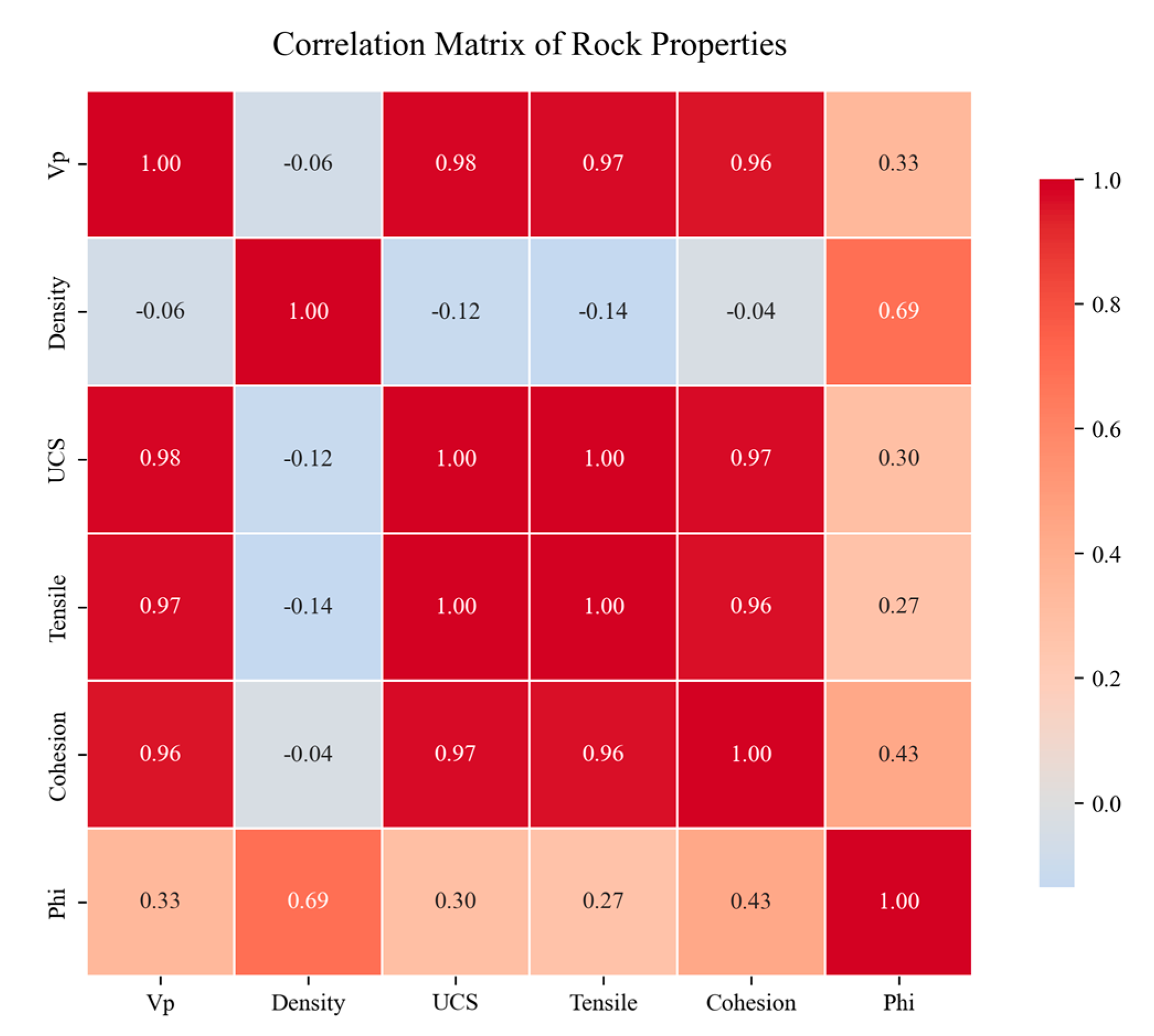
Figure 2.
Technical Roadmap of This Study Note: The left side shows the main workflow, while the right side displays the corresponding branch analyses for each stage; the dashed boxes indicate the three main research phases: model training and optimization, lithofacies analysis, and model interpretation and testing.
Figure 2.
Technical Roadmap of This Study Note: The left side shows the main workflow, while the right side displays the corresponding branch analyses for each stage; the dashed boxes indicate the three main research phases: model training and optimization, lithofacies analysis, and model interpretation and testing.
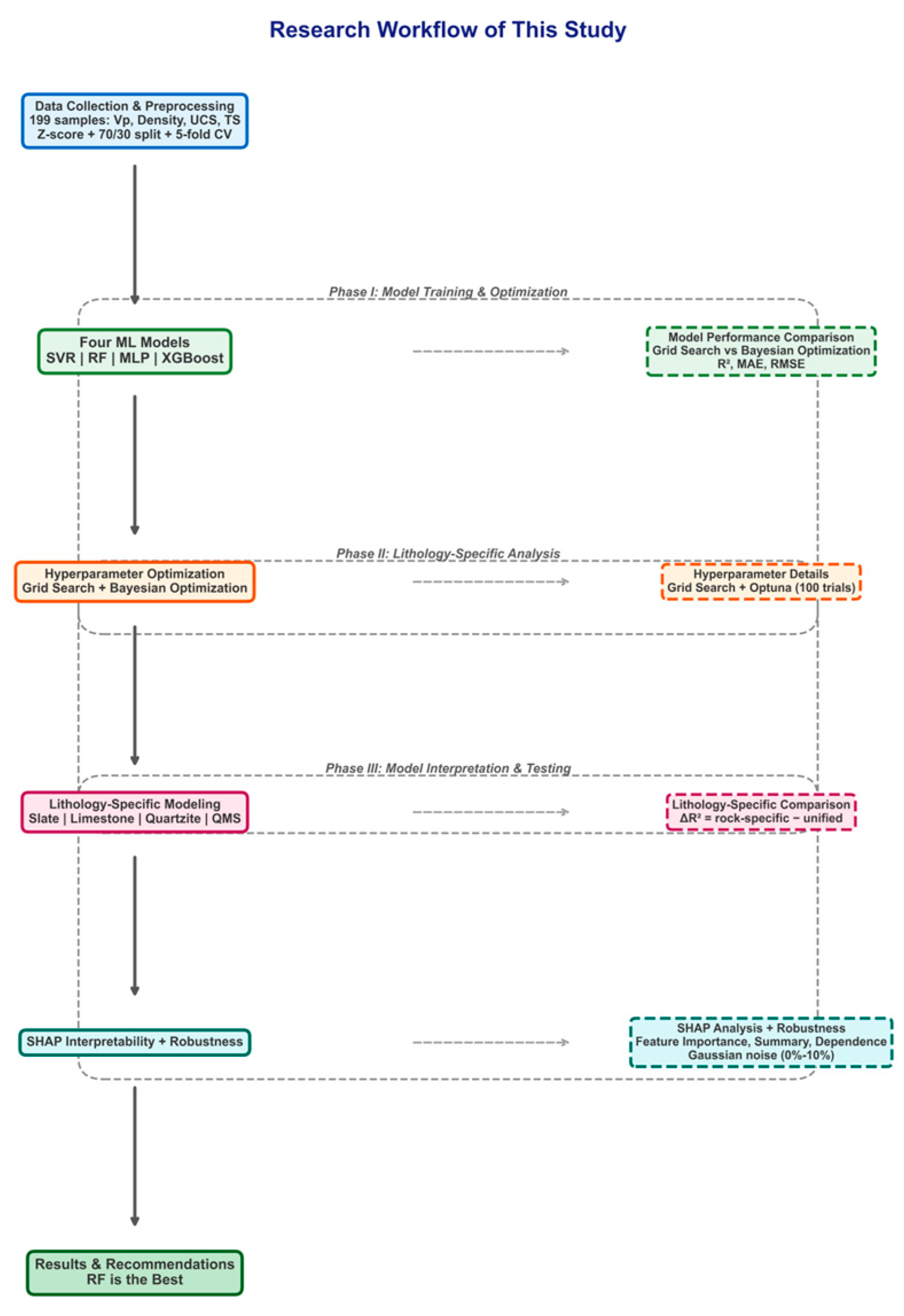
Figure 3.
Model Training Convergence Curve: (a) MLP training loss curve; the dashed line indicates entry into a plateau after approximately 500 iterations; (b) XGBoost validation RMSE curve; the dashed line indicates entry into a plateau after approximately 450 trees.
Figure 3.
Model Training Convergence Curve: (a) MLP training loss curve; the dashed line indicates entry into a plateau after approximately 500 iterations; (b) XGBoost validation RMSE curve; the dashed line indicates entry into a plateau after approximately 450 trees.
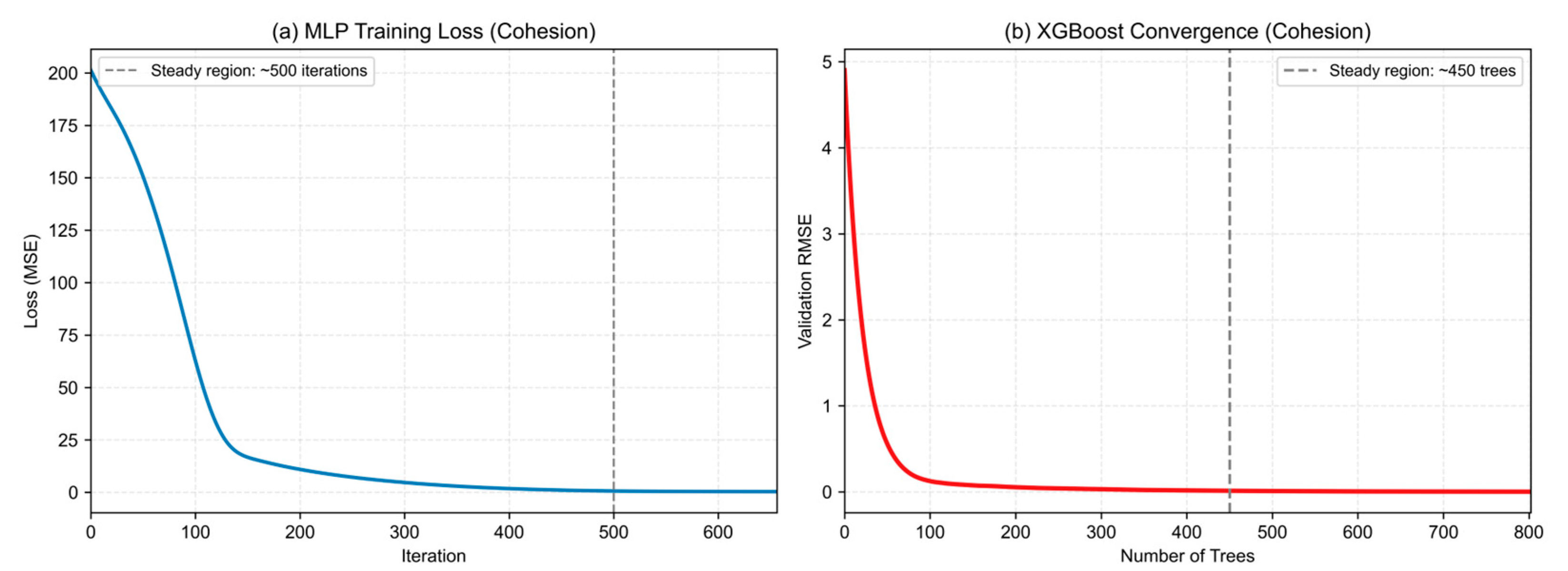
Figure 4.
Scatter plot of predicted and actual values for each model.
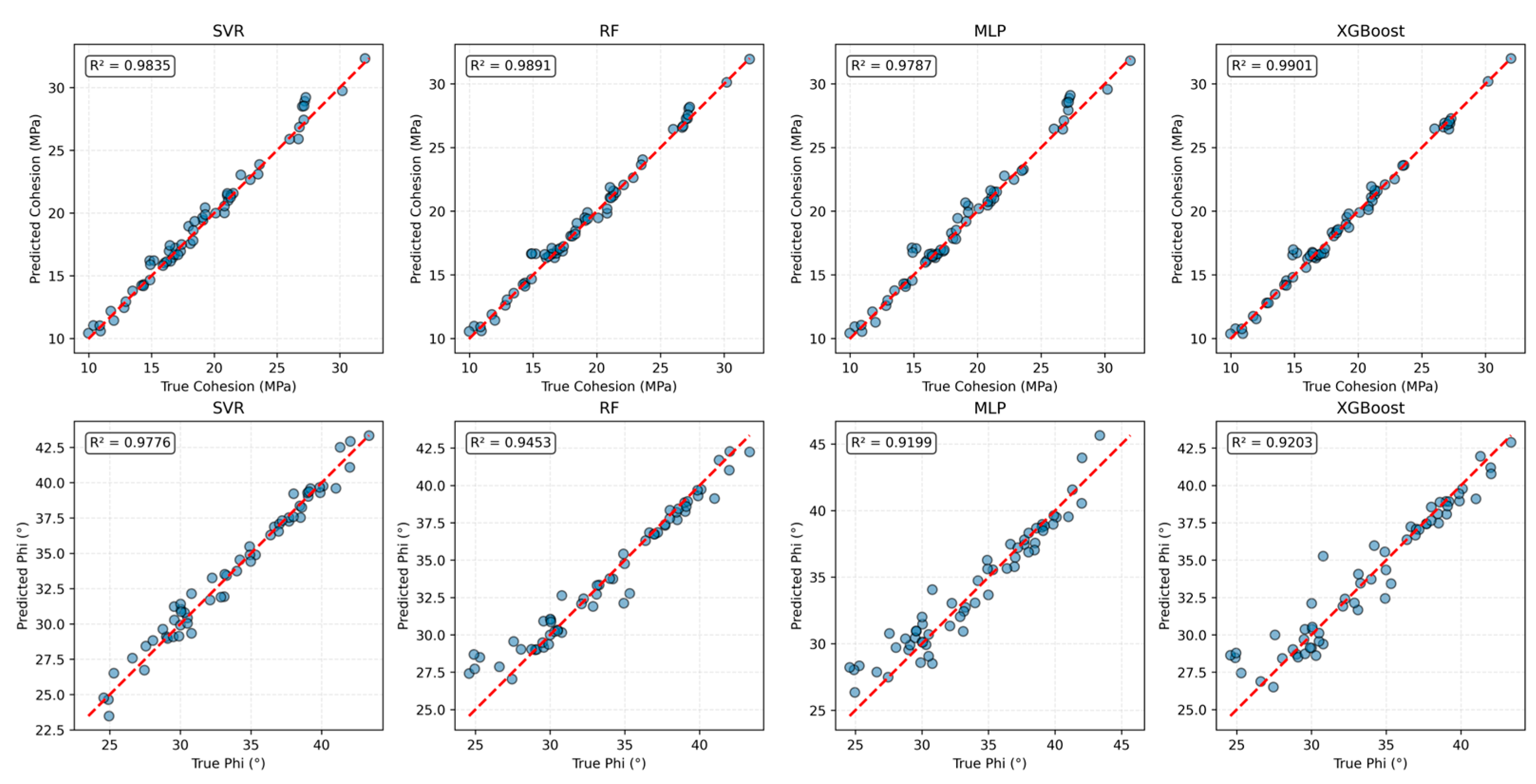
Figure 5.
Comparison of ΔR² between lithofacies-specific modeling and unified modeling (positive values indicate that lithofacies-specific modeling outperforms unified modeling).
Figure 5.
Comparison of ΔR² between lithofacies-specific modeling and unified modeling (positive values indicate that lithofacies-specific modeling outperforms unified modeling).
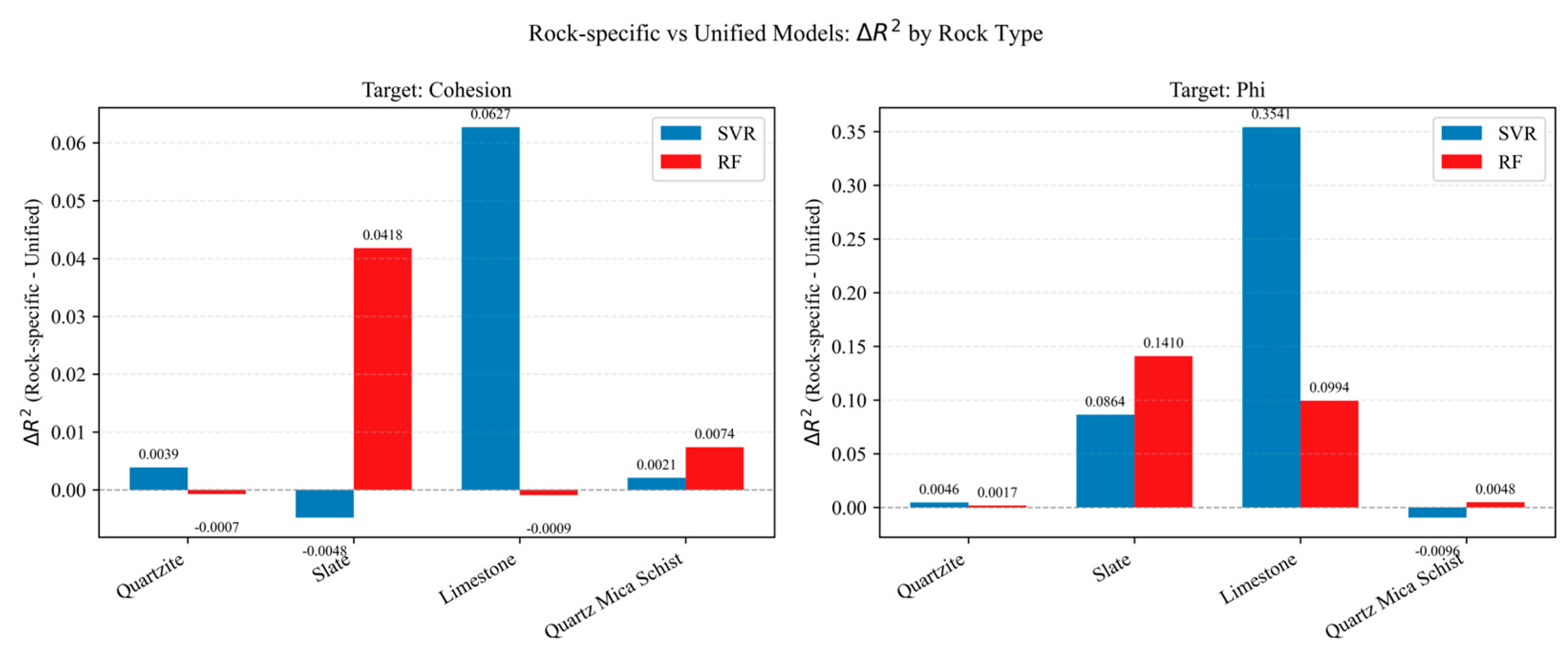
Figure 6.
SHAP analysis results: (a) XGBoost feature importance (
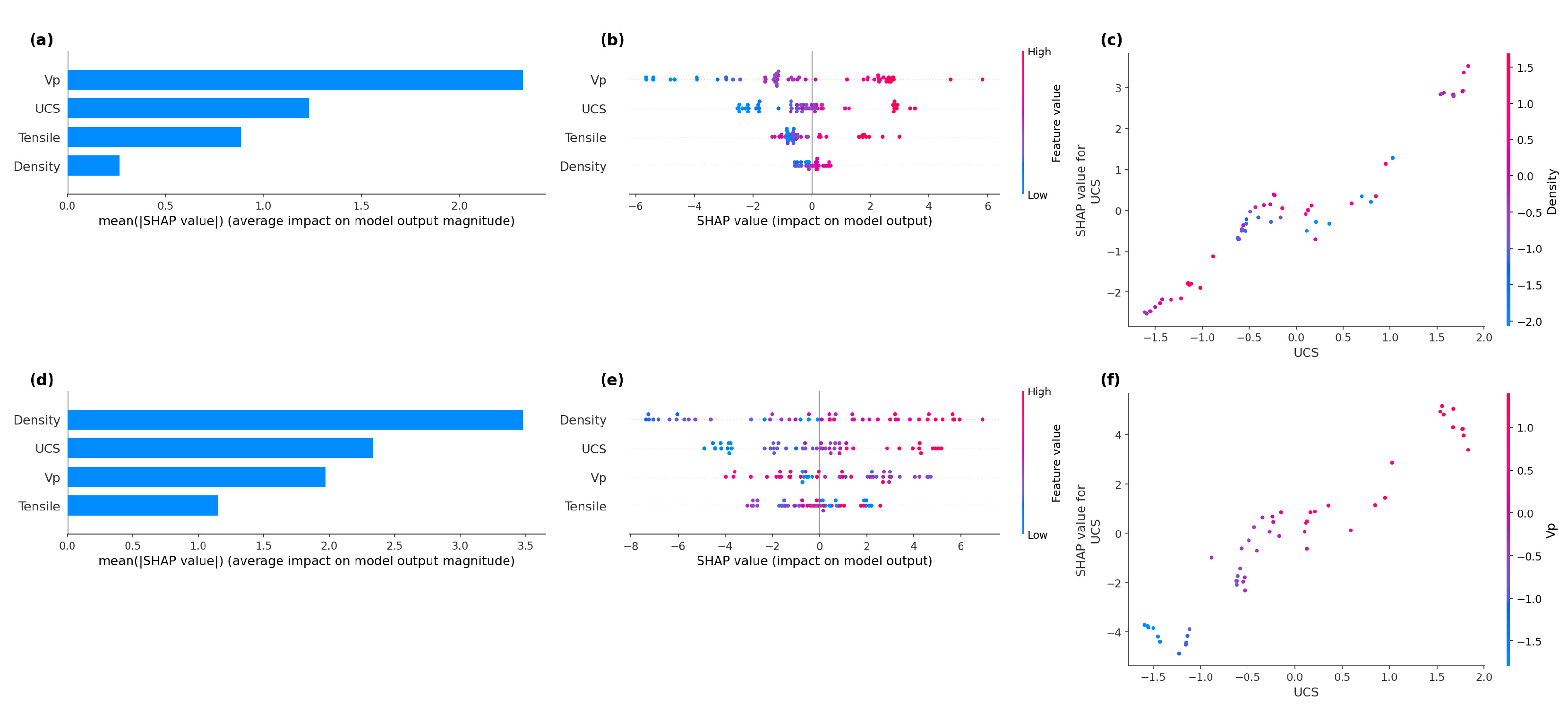
Figure 7.
Performance degradation curves of various models under different noise levels: (a) Cohesion
Figure 7.
Performance degradation curves of various models under different noise levels: (a) Cohesion
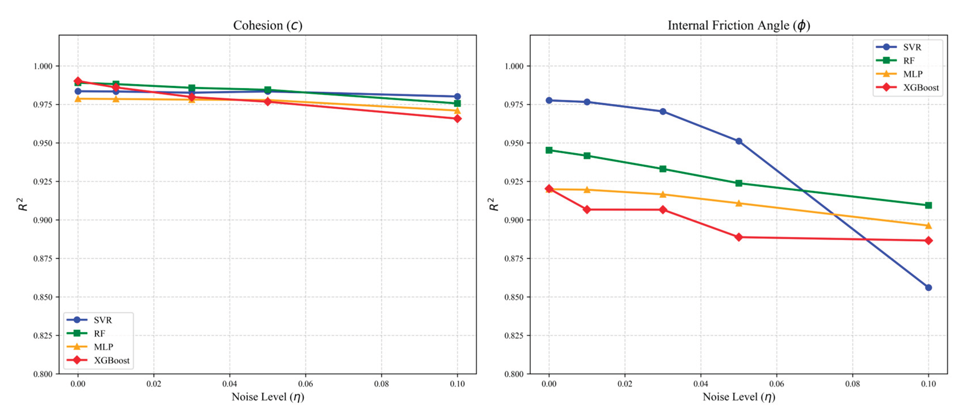

Table 1.
Representative Studies on Machine Learning for Predicting Rock Strength Parameters.
| Reference | Model | Input Parameters | Rock type | Prediction Target | Performance (R² or accuracy) |
| Kainthola et al.[14] | Linear regression, ANFIS | P-wave velocity | Shale, limestone, quartzite, quartz-mica schist | c, φ | ~0.95 |
| Shahani et al.[15] | Lasso, Ridge, Decision Trees, SVM | P-wave velocity, density, UCS, TS | Ibid. | c, φ | Optimal SVM: c = 0.977, φ = 0.916 |
| Mahmoodzadeh et al.[16] | GPR, SVR, decision trees, LSTM | UCS, UTS, σ₃ | Sandstone | c, φ | Good |
| Khandelwal et al.[18] | GA-ANN | P-wave velocity, UCS, TS | Limestone | c | R² = 0.967 |
| Hiba et al.[19] | Decision tree, random forest | Density, neutron porosity, compression time | Carbonate rock | c, φ | Error < 2.4% |
| Shen et al.[20] | Genetic programming | UCS, UTS, σ₃ | Sandstone | c, φ | Fair |
| Lei et al.[22] | ISSA-XGBoost | P-wave velocity, density, UCS, TS | Shale, limestone, quartzite, quartz-mica schist | c, φ | c = 0.982, φ = 0.932 |
| Jin et al.[21] | Data-driven + interpretability | Ibid. | Ibid. | c, φ | High accuracy |
| Verma et al.[23] | Evolutionary optimization of XGBoost | Multiple | Rock | c, φ | High accuracy |
| Xie et al.[24] | SSA-XGBoost | Feature optimization | Rock | UCS | — |
Table 2.
Statistical Characteristics of Input and Output Parameters.
| Parameter | Slate (n=50) | Limestone (n=49) | Quartzite (n=50) | Quartz-mica schist (n=50) |
| (m/s) | 4690.12 ± 623.37 | 4092.73 ± 429.83 | 5675.91 ± 373.94 | 2938.11 ± 464.85 |
| (g/cm³) | 2.68 ± 0.10 | 2.65 ± 0.07 | 2.59 ± 0.10 | 2.73 ± 0.06 |
| (MPa) | 141.53 ± 24.53 | 111.26 ± 14.04 | 198.53 ± 30.37 | 58.15 ± 10.12 |
| (MPa) | 17.85 ± 2.68 | 13.88 ± 1.76 | 24.89 ± 3.83 | 7.19 ± 1.09 |
| (MPa) | 19.13 ± 2.64 | 18.99 ± 1.73 | 25.80 ± 3.63 | 13.14 ± 1.60 |
| (°) | 31.53 ± 4.69 | 33.48 ± 2.99 | 35.95 ± 4.00 | 35.88 ± 4.26 |
Table 3.
Statistical Characteristics of Input and Output Parameters.
| Model | Hyperparameter | Candidate Values |
| SVR | 1, 10, 50, 100, 200 | |
| ‘scale’, ‘auto’, 0.01, 0.1 | ||
| 0.01, 0.05, 0.1 | ||
| RF | 100, 200, 300 | |
| None, 10, 20 | ||
| 2, 5 | ||
| 1, 2 | ||
| MLP | (32,), (64,), (64,32) | |
| 0.0001, 0.001, 0.01 | ||
| 0.001, 0.005, 0.01 | ||
| XGBoost | 100, 200, 300 | |
| 3, 5, 7 | ||
| 0.01, 0.05, 0.1 | ||
| 0.7, 0.8, 0.9 | ||
| 0.7, 0.8, 0.9 |
Table 4.
Bayesian optimization hyperparameter search ranges for each model.
| Model | Hyperparameter | Search Range | Distribution |
| SVR | [0.1, 1000] | Log-uniform | |
| [1e-4, 0.5] | Log-uniform | ||
| [0.01, 0.5] | Logarithmic uniform | ||
| RF | [50,300] | Integer uniform | |
| [3, 20] | Uniformly distributed integers | ||
| [2, 10] | Uniformly distributed integers | ||
| [1, 10] | Uniformly distributed integers | ||
| MLP | (32,), (64,), (32,16) | Class | |
| [1e-4, 0.1] | Logarithmic uniform | ||
| [1e-4, 5e-3] | Log-uniform | ||
| XGBoost | [100, 400] | Integer uniform | |
| [3, 8] | Uniformly distributed integers | ||
| [0.01, 0.3] | Uniform | ||
| [0.7, 1.0] | Uniform | ||
| [0.7, 1.0] | Uniform | ||
| [0,1] | Uniform | ||
| [1e-8, 0.1] | Log-uniform | ||
| [0.5, 2.0] | Uniform |
Table 5.
Comparison of Test Set Performance Between Grid Search and Bayesian Optimization.
| Model | Objective | Grid Search R² | Bayesian Optimization R² | Final Selection |
| SVR | c | 0.9835 | 0.9831 | Grid |
| SVR | φ | 0.9176 | 0.9776 | Bayesian |
| RF | c | 0.9891 | 0.9890 | Grid |
| RF | φ | 0.9453 | 0.9411 | Grid |
| MLP | c | 0.9504 | 0.9787 | Bayesian |
| MLP | φ | 0.9033 | 0.9199 | Bayesian |
| XGBoost | c | 0.9901 | 0.9855 | Grid |
| XGBoost | φ | 0.9203 | 0.9151 | Grid |
Table 6.
Comparison of
| Rock Type | Model | Target | Rock-type-specific | Unification | |
|---|---|---|---|---|---|
| Quartzite | SVR | c | 0.9338 | 0.9299 | +0.0039 |
| Quartzite | RF | c | 0.9764 | 0.9770 | -0.0007 |
| Quartzite | SVR | φ | 0.9694 | 0.9648 | +0.0046 |
| Quartzite | RF | φ | 0.9891 | 0.9875 | +0.0017 |
| Slate | SVR | c | 0.9210 | 0.9258 | -0.0048 |
| Slate | RF | c | 0.9478 | 0.9060 | +0.0418 |
| Slate | SVR | φ | 0.9751 | 0.8887 | +0.0864 |
| Slate | RF | φ | 0.9726 | 0.8317 | +0.1410 |
| Limestone | SVR | c | 0.9626 | 0.8999 | +0.0627 |
| Limestone | RF | c | 0.9685 | 0.9694 | -0.0009 |
| Limestone | SVR | φ | 0.9495 | 0.5954 | +0.3541 |
| Limestone | RF | φ | 0.9738 | 0.8744 | +0.0994 |
| Quartz-mica schist | SVR | c | 0.9679 | 0.9657 | +0.0021 |
| Quartz-mica schist | RF | c | 0.9734 | 0.9659 | +0.0074 |
| Quartz-mica schist | SVR | φ | 0.9694 | 0.9790 | -0.0096 |
| Quartz-mica schist | RF | φ | 0.9770 | 0.9721 | +0.0048 |
Table 7.
Guidelines for the Engineering Application of Rock Strength Parameter Prediction.
| Condition Dimensions | Specific Scenarios | Recommended Model | Expected Performance | Basis for Decision-Making |
| Data Quality | High quality (standard indoor testing) | c: XGBoost φ: SVR (Bayesian) |
c: R² ≥ 0.990 φ: R² ≥ 0.975 |
Pursuing Maximum Accuracy (Table 5) |
| Moderate accuracy (including field test errors) | Random Forest (RF) | c: R² ≈ 0.989 φ: R² ≈ 0.945 |
Optimal balance between accuracy and robustness (Figure 7) | |
| Low quality (missing parameters or high noise) | Random Forest (RF) | Depends on the missing data situation | Tree models are insensitive to noise and missing features | |
| Lithological conditions | Limestone (uniform structure) | Lithology-specific modeling (SVR/RF) | φ: R² can be improved to ≥0.95 | ΔR² as high as 0.3541 (Table 6) |
| Slate (metamorphic schistosity) | Lithofacies modeling (φ only) | φ: R² can be increased to ≥0.12 | RF diagenetic ΔR² = 0.1410 (Table 6) | |
| Quartzite/Quartz-Mica Schist | Unified Model | Consistent with Table 5 | No significant improvement by lithology (ΔR² < 0.01) | |
| Prediction target | Prioritize predicting cohesion c | XGBoost (grid search) | R² = 0.9901 | Table 5: Optimal Accuracy |
| Prioritize predicting the internal friction angle φ | SVR (Bayesian Optimization) | R² = 0.9776 | Table 5: Optimal Accuracy | |
| Balancing Both | Random Forest (RF) | c: 0.9891, φ: 0.9453 | Best Overall Performance (Table 5 + Figure 7) | |
| Data Features | Input parameters contain measurement noise | Random Forest (RF) | R² decreases by <0.04 under 10% noise | Strongest noise resistance (Figure 7) |
| Only UCS and UTS | XGBoost or RF | Slightly lower than all features | Strength metrics as the core (Figure 6) |
* Note: Expected performance is based on the results of this paper’s test set; actual performance in engineering applications may vary due to differences in data.
Disclaimer/Publisher’s Note: The statements, opinions and data contained in all publications are solely those of the individual author(s) and contributor(s) and not of MDPI and/or the editor(s). MDPI and/or the editor(s) disclaim responsibility for any injury to people or property resulting from any ideas, methods, instructions or products referred to in the content. |
© 2026 by the authors. Licensee MDPI, Basel, Switzerland. This article is an open access article distributed under the terms and conditions of the Creative Commons Attribution (CC BY) license.
Copyright: This open access article is published under a Creative Commons CC BY 4.0 license, which permit the free download, distribution, and reuse, provided that the author and preprint are cited in any reuse.


