

Submitted:
24 July 2026
Posted:
27 July 2026
You are already at the latest version
Abstract
Partial least squares structural equation modeling (PLS-SEM) is a widely used method in behavioral and social science research, but its use is limited by software access and specialized desktop software. AnalyVa is a desktop statistical analysis platform (offline, locally installed) based on Electron that provides complete PLS-SEM capabilities, such as reflective model estimation, moderation analysis, and second-stage interaction modeling, without the need for internet connection or programming skills. This tutorial compares AnalyVa with the current reference standard, SmartPLS 4, for three model specifications: (1) a simple four-construct reflective model, (2) an extended moderation model with one multi-item moderator, and (3) a multiple interaction model with three single-item moderators and all higher-order interaction terms. We compare outer loadings, construct reliability and validity, discriminant validity (HTMT and Fornell-Larcker criterion), structural path coefficients, effect sizes (f²), and model fit indices (SRMR and NFI) using an existing data set (n = 344) from the corporate reputation literature. Results show good agreement, with the largest absolute differences being less than .010 for path coefficients and less than .006 for outer loadings for all three models. Systematic divergences in model fit reporting are identified and explained: AnalyVa separately reports saturated and estimated model fit indices—a distinction SmartPLS 4 collapses for simple models. AnalyVa’s Smart Model Health diagnostics flagged an elevated outer VIF in the extended moderation model not surfaced by SmartPLS 4. The results indicate that AnalyVa is a methodologically sound and diagnostically useful desktop alternative to PLS-SEM practitioners.
Keywords:
PLS-SEM
; AnalyVa
; SmartPLS
; software validation
; moderation
; interaction effects
; behavioral research methods
Introduction
Partial least squares structural equation modeling (PLS-SEM) has become a popular method in behavioral, management, and information systems research (Hair et al., 2022; Ringle et al., 2020). It is particularly valuable in situations where the sample size is small, the data are not normally distributed, and the models involve multiple latent variables and intricate relationships between them. The most widely used software in this field is SmartPLS, which is currently in version 4 (Ringle et al., 2024), and has the largest user base and the strongest presence in methodological development.
Despite the widespread availability of SmartPLS, researchers increasingly seek alternative validated platforms for PLS-SEM. AnalyVa (https://analyva.com) addresses this by delivering full PLS-SEM functionality—including reflective model estimation, moderation analysis, and second-stage interaction modeling—through a locally installed Electron-based desktop application that does not require internet connectivity.
For any new analytical tool to gain scientific traction, it must demonstrate empirical equivalence with established reference implementations. Validation studies comparing software platforms are well-established in adjacent literatures: for example, comparisons of R, SAS, and SPSS for regression and ANOVA (Gettman, 2010; Sharma, 2025), a comparison of SPSS with an AI-based analysis tool, ChatGPT-4 (Shahrul & Syed Mohamed, 2024), or comparisons of Mplus and LISREL for covariance-based SEM (Byrne, 2012). Within PLS-SEM, such cross-software validation studies are comparatively rare, and none, to our knowledge, have examined a desktop implementation against SmartPLS.
This paper addresses that gap. We systematically compare AnalyVa and SmartPLS 4 using an established dataset (n = 344) and three model specifications: a simple reflective model, an extended moderation model, and a model with multiple simultaneous interaction terms. Rather than re-interpreting the substantive findings of the original analyses—which have been reported elsewhere in the literature—we focus on the numerical concordance (and any discordance) of the outputs produced by each platform. We also draw attention to a key differentiating feature of AnalyVa: its automated Smart Model Health diagnostics, which proactively surface model quality concerns beyond those typically reported by SmartPLS 4. Although the illustrative dataset used here is drawn from the corporate reputation literature, PLS-SEM is increasingly applied across behavioral and cognitive research contexts—including studies of learning motivation, self-regulation, technology acceptance, and health behavior—making accessible, valid tooling directly relevant to BRM’s readership.
Background
PLS-SEM: Overview and Software Landscape
PLS-SEM is a composite-based structural equation modeling technique that estimates relationships among latent constructs represented by indicator variables (Hair et al., 2019). The algorithm iteratively computes construct scores as linear combinations of their indicators, then estimates structural paths between constructs via ordinary least squares regression. Its main strengths include handling non-normal data distributions, high statistical power relative to covariance-based SEM in small-to-medium samples, and flexibility in managing both reflective and formative measurement models (Sarstedt et al., 2021).
SmartPLS (Ringle et al., 2024) is widely regarded as the leading software for PLS-SEM estimation. Since its initial release, it has offered a graphical model builder, extensive output reports covering measurement model assessment, structural inference, bootstrapping, and moderation analysis. SmartPLS 4 introduced improved diagnostics, a refined second-stage moderation procedure, and expanded model selection criteria. Other PLS-SEM-capable tools include WarpPLS (Kock, 2022) and the SEMinR package for R (Ray et al., 2022), each with distinct design philosophies.
Moderation in PLS-SEM
Moderation analysis in PLS-SEM involves testing whether the effect of one construct on another varies as a function of a third (moderating) variable (Hair et al., 2022). The product-indicator approach, two-stage approach, and orthogonalizing approach each offer different trade-offs between bias and efficiency (Henseler & Chin, 2010). SmartPLS 4 primarily implements the two-stage approach for extended moderation: in the first stage, construct scores are estimated from the base model; in the second stage, the interaction term is constructed from the product of the moderator and predictor scores and added to the structural model. AnalyVa likewise implements this two-stage approach, ensuring methodological comparability.
In complex models where multiple moderators and their higher-order interaction terms are included simultaneously, the number of interaction constructs grows combinatorially. For three binary moderators, there are 3 main effects, 3 two-way interactions, 1 three-way interaction, and (if an additional continuous moderator such as LIKE is included) another 7 new interaction terms (plus LIKE as a fourth main effect), totaling 15 moderation-related paths (4 moderator main effects plus 11 interaction product terms). Both SmartPLS 4 and AnalyVa support such specifications, and their numerical agreement in this high-complexity scenario is a stringent test of equivalence.
Validation Framework for Computational Tools
The validation of software in quantitative research methods usually involves comparing the estimates of the parameters, the standard errors, and the goodness-of-fit statistics from different implementations of the same method on the same data set with a known solution. Estimates that are near identical with small absolute differences (usually |Δ| < .01 for standardized coefficients) are evidence of equivalent computation. Systematic differences in reporting conventions (e.g., different formulae for reliability coefficients or different model specifications for fit indices) should be considered methodological features and explicitly reported.
AnalyVa: Features and Capabilities
AnalyVa is a desktop application that can be accessed at https://analyva.com and is based on Electron. Users start by uploading structured CSV data, and then create the PLS-SEM model in a point-and-click interface by creating constructs, connecting indicators, and defining structural paths. No statistical programming or command-line skills are needed. It allows for reflective and composite measurement models, second-stage extended moderation, multiple simultaneous interaction terms, and a variety of post-estimation diagnostics.
Smart Model Health Diagnostics
One of the unique characteristics of AnalyVa is the automated Smart Model Health panel that is shown as soon as the model is estimated. The panel groups diagnostic findings into three severity levels: High (red), Review (orange), and Info (blue). Results may involve high outer model VIF values (which suggest that indicators are redundant), inner model VIF concerns (which suggest structural multicollinearity), model fit threshold violations, and data quality problems (e.g., missing values). Importantly, this diagnostic layer is not user-driven (a health report is generated with every estimation run), which reduces the hurdle for identifying model specification issues, especially for researchers who are not as well-versed in the PLS-SEM assumptions.
Output and Reporting
AnalyVa generates tabular output covering: (a) outer loadings and weights, (b) construct reliability (Cronbach’s alpha [α], composite reliability [ρa and ρc]), and average variance extracted (AVE), (c) discriminant validity via both the heterotrait-monotrait ratio (HTMT; Henseler et al., 2015) and the Fornell-Larcker criterion, (d) inner model VIF, (e) path coefficients with effect size (f²), (f) R² and adjusted R², and (g) model fit indices (SRMR, d_ULS, χ², NFI) for both the saturated and estimated models. A copy button is provided in each output table in APA format and a status classification is provided based on thresholds. AnalyVa also provides interaction effect size and graphical slope plots for moderation analyses.
Moderation Estimation Approach
In single-moderator models, AnalyVa uses the two-stage extended moderation approach as implemented in SmartPLS 4: the first stage involves estimating construct scores from the structural model without the interaction term, while the second stage involves adding the product of the moderator and predictor construct scores as a single-indicator interaction construct. AnalyVa generates all desired higher order product terms in one estimation pass for multiple simultaneous moderators. For validation to be meaningful, operational equivalence with SmartPLS 4 must first be established.
Method
Dataset
The analyses use the corporate reputation dataset provided with SmartPLS 4 as a canonical example dataset, which has been analyzed and reported in multiple methodological publications (Sarstedt et al., 2014; Hair et al., 2017). The dataset consists of n = 344 complete cases (after mean replacement of 11 missing values, which were the same across both platforms) and measures constructs from the European Customer Satisfaction Index (ECSI) framework: Attractiveness (ATTR; 3 items), Corporate Social Responsibility (CSOR; 5 items), Performance (PERF; 5 items), Quality (QUAL; 8 items), Competence (COMP; 3 items), Likability (LIKE; 3 items), Customer Satisfaction (CUSA; single item), Customer Loyalty (CUSL; 3 items), and Switching Barriers (SWITCH; 4 items in the extended model, or three separate single-item constructs [SWITCH1, SWITCH2, SWITCH3] in the multiple interaction model). All items use seven-point Likert-type scales.
Model Specifications
Three model specifications were estimated in both SmartPLS 4 and AnalyVa:
Model 1—Simple Reflective Model. A four-construct model with COMP and LIKE as exogenous constructs, CUSA as a mediating construct, and CUSL as the endogenous outcome. Hypothesized paths are COMP → CUSA, COMP → CUSL, LIKE → CUSA, LIKE → CUSL, and CUSA → CUSL.
Model 2—Extended Moderation Model. An expanded version of Model 1 that includes four antecedent constructs (ATTR, CSOR, PERF, QUAL) predicting COMP and LIKE, and adds a multi-item SWITCH construct as a moderator of CUSA → CUSL. The interaction term SWITCH × CUSA is constructed using the two-stage approach.
Model 3—Multiple Interaction Model. This model retains the core Model 1 structure and introduces three single-item constructs (SWITCH1, SWITCH2, SWITCH3) as simultaneous moderators of CUSL, along with LIKE as an additional moderator. All two-way, three-way, and four-way interaction terms are constructed, yielding 15 moderation-related paths to CUSL (comprising 4 moderator main effects and 11 two-way, three-way, and four-way interaction product terms) in addition to the baseline structural paths.
Analysis Procedure
Identical datasets (CSV format) were uploaded to both SmartPLS v4.1.1.8 and AnalyVa. Models were specified identically in each platform. For both tools, the PLS-SEM algorithm used path weighting, standardized results, default initial weights, mean replacement for missing values, and a convergence criterion of 1.0 × 10⁻⁷. Both platforms used the two-stage approach for moderation. Bootstrapping for significance testing was not conducted in this study, as the objective is parameter concordance rather than inference; previous publications using this dataset provide inferential conclusions (Sarstedt et al., 2014; Hair et al., 2017). Output values were extracted from the SmartPLS Excel report and the AnalyVa results spreadsheet. Absolute differences (Δ) between matched parameter estimates are reported to facilitate direct comparison.
Results
Model 1: Simple Reflective Model
Measurement Model Assessment
The outer loadings for the simple reflective model are shown in Table 1. In both platforms, all indicator loadings are greater than .70, and the values are highly concordant, with the largest absolute difference being .006. As expected, the single-item CUSA construct loads at 1.000 in both platforms.
Table 2 presents construct reliability and validity statistics. Cronbach’s alpha (α) values are identical across platforms for all constructs, as this coefficient is a function of the correlation matrix and is computed identically. Composite reliability (ρc) values are also identical or differ by at most .001. The primary difference lies in the reliability coefficient rho_a (ρa): AnalyVa reports slightly higher values than SmartPLS 4 (e.g., COMP: .847 vs. .832; CUSL: .891 vs. .839). This difference is due to a known implementation difference in the ρa formula originally proposed by Dijkstra and Henseler (2015): AnalyVa applies the diagonal correction to the outer weight matrix before squaring, while SmartPLS 4 applies it after, which results in systematically higher ρa values in AnalyVa. The values of both platforms are still above .70. However, all values in both platforms are above the recommended value of .70 (Hair et al., 2019), and all AVE values are above .50, which is the threshold for convergent validity.
Table 3 presents the HTMT ratios. All values are virtually identical between platforms (differences ≤ .001), and all pairs fall below the conservative .85 threshold, supporting discriminant validity. The Fornell-Larcker criterion was also satisfied in both platforms: the square root of each construct’s AVE (diagonal values) exceeded all inter-construct correlations in its row and column.
Structural Model Assessment
Table 4 presents the structural model results. Path coefficients are consistent to three decimal places for all five hypothesized paths, with the largest difference being .002. The indirect effects (COMP → CUSA → CUSL and LIKE → CUSA → CUSL) are likewise near-identical. R² values are equivalent to three decimal places for both endogenous constructs. Effect sizes (f²) are likewise highly concordant, with a maximum difference of .004 (for CUSA → CUSL: SmartPLS = .410, AnalyVa = .406).
Table 5 presents model fit indices for all three models. Both platforms give the same SRMR for the saturated model (.074), which indicates that the reproduced correlation matrix is the same. However, AnalyVa reports an estimated model SRMR of .103, compared to SmartPLS 4’s .074 for the estimated model. This difference is due to the fact that the two platforms have different definitions of the implied correlation matrix of the estimated model: In this model structure, the SRMR value is the same for both model variants in SmartPLS 4, which assumes that the model is saturated in the simple case, while AnalyVa enforces the constraint that only the hypothesized paths contribute to the reproduced correlation matrix, resulting in a higher (and more conservative) estimated model SRMR. The NFI also shows this difference: .820 for SmartPLS 4 and .818 (saturated) and .758 (estimated) for AnalyVa. Researchers should be aware that AnalyVa’s estimated model SRMR provides a stricter criterion for model parsimony.
Model 2: Extended Moderation Model
Table 6 presents path coefficients for the extended moderation model. Agreement between platforms is strong: 13 of 15 paths differ by .002 or less, and the maximum absolute difference is .005 (CUSA → CUSL: SmartPLS β = .467, AnalyVa β = .462; and SWITCH → CUSL: SmartPLS β = .070, AnalyVa β = .075). The moderation effect (SWITCH × CUSA → CUSL) is effectively identical: SmartPLS β = −.071, AnalyVa β = −.072. R² values are equivalent across all four endogenous constructs.
The extended model measurement model statistics are also consistent. The SWITCH construct (four items: switch_1 through switch_4) shows identical Cronbach’s alpha (α = .858 in both platforms), composite reliability (ρc = .905), and AVE (.705), with small differences in ρa (.892 vs. .858). All loadings for SWITCH items exceed .74 in both platforms, and HTMT values between SWITCH and the other constructs are all below .85.
A notable differentiating output of AnalyVa is its Smart Model Health diagnostic, which flagged two “High” severity findings for the extended model:
1. Two outer VIF values at or above 5: switch/switch_1 = 31.122; switch/switch_4 = 30.706.
2. Two inner VIF values between 3.3 and 5: qual → comp = 3.490; qual → like = 3.490.
The extreme outer VIF values for the SWITCH indicators switch_1 and switch_4 indicate that these two items are almost perfectly multicollinear in the outer model context, which is probably due to the high inter-item correlation of the four items in the switching barriers scale. By default, SmartPLS 4 did not generate an alert for the corresponding issue, but rather left it up to the user to check the VIF values. If outer VIF values are above 5, practitioners may want to remove one of the redundant indicators (the one with the highest loading or the highest content validity), or respecify the construct as a formative measurement model if theoretically appropriate, or merge highly overlapping indicators into a parcel. This is a good example of a practical benefit of AnalyVa’s automated diagnostics for researchers who might not be checking individual outer VIF values on a regular basis.
Figure 2a and Figure 2b show the path model diagrams for the extended moderation model from AnalyVa and SmartPLS 4, respectively. Both display the same structural topology with the interaction term (SWITCH × CUSA) linking to CUSL.
As can be seen in Table 5, the model fit of the extended model varies more significantly across platforms: SmartPLS 4 reports SRMR = .063/.064 and NFI = .605, while AnalyVa reports SRMR = .067/.075 and NFI = .559/.542. The addition of antecedent constructs (ATTR, CSOR, PERF, QUAL) and the moderation product term significantly expands the model and adds more residualized relationships. The discrepancy in NFI, which is sensitive to the number of free parameters compared to the saturated model, may be due to differences in the second-stage estimation procedure for the interaction term, namely how the product scores are standardized before they are included.
Model 3: Multiple Interaction Model
The multiple interaction model is the most stringent test of cross-platform equivalence, involving three single-item moderator constructs (SWITCH1, SWITCH2, SWITCH3) and LIKE as a fourth moderator, generating 11 interaction product terms (plus 4 moderator main effects, totaling 15 moderation-related paths) predicting CUSL. Table 7 presents all path coefficients. Agreement is again strong: 17 of 19 reported paths differ by .003 or less. The largest discrepancies are for SWITCH1 → CUSL (SmartPLS = .052, AnalyVa = .061; Δ = .009) and SWITCH3 × SWITCH1 → CUSL (SmartPLS = −.089, AnalyVa = −.096; Δ = .007). These slightly larger discrepancies for higher-order interaction terms likely reflect minor differences in the numerical precision of the product score construction at higher levels of multiplication. R² values are identical: CUSA = .295, CUSL = .597 in both platforms.
An interesting pattern emerges in the model fit indices for this model (Table 5). AnalyVa reports considerably better fit: SRMR(sat) = .041 and NFI(sat) = .933, compared to SmartPLS 4’s SRMR(sat) = .063 and NFI(sat) = .848. This divergence is attributable to how each platform constructs the correlation matrix for SRMR and NFI computation when product-indicator constructs are single-indicator constructs with trivially perfect loadings. When the model contains a large number of such unit-loading interaction constructs (as is the case here with 11 product terms), the denominator of the residual matrix diverges between platforms depending on whether product term indicators are included in or excluded from the implied correlation matrix used for fit computation. Based on AnalyVa’s documented computation, the platform restricts the SRMR calculation to substantive (multi-indicator) constructs, excluding trivially unit-loading product-indicator constructs from the implied correlation matrix, while SmartPLS 4 includes all construct scores. Neither approach is inherently incorrect; they answer subtly different questions about model fit.
Discussion
Overall Concordance
Across three PLS-SEM model specifications of increasing complexity, AnalyVa and SmartPLS 4 produced near-identical parameter estimates. For the simple reflective model, absolute differences in path coefficients never exceeded .002, and outer loadings differed by at most .006. For the extended moderation model, the largest discrepancies in structural paths were .005, which is within the range of equivalence for standardized coefficients. In the complex multiple interaction model (19 total estimated paths, including 15 moderation-related paths and 4 core structural paths from Table 7), the largest absolute difference was .009, which was due to numerical compounding in the construction of higher-order product terms. Across all three models, R² values were identical or differed by at most .002. All these findings together indicate that AnalyVa fully applies the PLS-SEM algorithm and the two-stage moderation procedure for substantive parameter estimation as in SmartPLS 4.
Differences in Reliability Reporting: ρa
The most consistent cross-platform difference was found in the rho_a (ρa) reliability coefficient, which was systematically higher in AnalyVa than in SmartPLS 4 (e.g., COMP: .847 vs. .832). Both values are well above the recommended threshold of .70, and the implications for conclusions about the quality of measurement are not significant. The divergence is due to a particular implementation difference in the formula for ρa (Dijkstra & Henseler, 2015): the diagonal correction applied to the outer weight matrix is different for the two platforms. This distinction should be taken into account by researchers reporting from AnalyVa when comparing ρa values directly to the benchmarks derived from SmartPLS.
Model Fit Indices: Saturated vs. Estimated
The biggest methodological difference between the platforms is in the reporting of model fit. For the simple model, both platforms produced the same saturated-model SRMR (.074), which indicates that they reproduced the correlation matrix equivalently. AnalyVa’s estimated model SRMR (.103) is higher than SmartPLS 4’s (.074) because AnalyVa enforces a strict estimated model computation: only hypothesized paths contribute to the implied model-predicted correlation matrix. In this instance, SmartPLS 4 reports the same values for both model variants, which might be a default behavior when the model structure is fully identified. For applied users, AnalyVa’s estimated SRMR appears to provide a more conservative assessment of structural model parsimony, and one that is arguably more meaningful, consistent with Henseler et al. (2016).
For the extended and multiple interaction models, fit index divergences were larger (particularly NFI) and likely stem from differing treatments of interaction term constructs in the model size normalization. Because NFI is sensitive to model complexity (number of free parameters vs. null model), including or excluding trivially perfect-loading product constructs from the NFI denominator produces substantially different values. The choice of computation should be considered when interpreting NFI values from complex moderation models in AnalyVa.
Smart Model Health: A Diagnostic Advantage
A practically significant differentiating feature of AnalyVa is the Smart Model Health panel. In the extended moderation model, AnalyVa automatically flagged outer VIF values exceeding 5 for two SWITCH indicators (VIF(switch_1) = 31.122; VIF(switch_4) = 30.706). These extreme values indicate near-redundancy between switch_1 and switch_4, which share substantial item content. SmartPLS 4 did not surface a corresponding default alert. For researchers who do not routinely inspect outer VIF tables, this automated early-warning system meaningfully lowers the risk of publishing results based on a multicollinear measurement model without acknowledgment.
Practical Implications
For behavioral researchers, the primary implication of this validation is that AnalyVa is a credible tool for PLS-SEM estimation with results that are numerically equivalent to SmartPLS 4 for substantive parameters. The locally installed architecture makes it especially suitable for classroom instruction, cross-institutional collaboration, and deployment in data-sensitive or connectivity-constrained research environments. The automated diagnostic layer makes it suitable for researchers at earlier stages of PLS-SEM competency who benefit from guided model quality feedback. The SRMR divergence in complex moderation models warrants awareness but does not compromise the validity of structural estimates.
Limitations
This validation used a single, well-established dataset. Generalizability to datasets with different distributional properties, larger or smaller sample sizes, or formative measurement models should be established in future work. Bootstrapping-based inference (t-statistics, p-values, confidence intervals) was not assessed here, as the focus was on algorithm-level parameter concordance; accordingly, no measures of variability around parameter estimates are reported. This is a computational equivalence study, not an inferential study, and this scope is explicitly acknowledged. Future studies should compare bootstrapped significance results between platforms, including consistency at low iteration counts. Additionally, this study focused on reflective constructs and product-indicator interaction terms; second-order constructs and non-linear relationships (higher-order PLS-SEM specifications) merit separate validation.
Conclusions
This tutorial provides the first systematic cross-platform validation of AnalyVa, an Electron-based desktop PLS-SEM platform (offline, locally installed), against SmartPLS 4—the established reference standard. Across simple reflective, extended moderation, and multiple interaction models estimated on an established corporate reputation dataset (n = 344), AnalyVa produced parameter estimates in strong agreement with SmartPLS 4, with maximum absolute path coefficient differences below .010. Systematic differences in model fit reporting are attributable to methodological choices—notably AnalyVa’s stricter estimated-versus-saturated model distinction—rather than computational errors, and do not affect substantive conclusions about structural relationships. AnalyVa’s automated Smart Model Health diagnostics provide a practitioner-oriented advantage by surfacing model quality concerns (such as outer VIF violations) without requiring manual inspection. Together, these findings support the use of AnalyVa as a valid, accessible, and diagnostically informative platform for PLS-SEM research in behavioral and social sciences.
Authors’ contributions
A.B. conceived the study and developed AnalyVa. K.E. and A.B. conducted the validation analyses. All authors contributed to the manuscript and approved the final version.
Consent for publication
Not applicable.
Ethics approval
Not applicable. This article uses a publicly available, anonymized secondary dataset and does not involve human participants.
Availability of data and materials
The dataset analysed during the current study is the SmartPLS 4 example dataset, publicly available at https://www.smartpls.com. AnalyVa output files (results spreadsheets for all three models) are publicly archived at Mendeley Data through https://doi.org/10.17632/y776mr82vs.1 in accordance with BRM’s Type 4 data policy.
Conflicts of interest/Competing interests
A.B. is the principal developer of AnalyVa. As AnalyVa is distributed commercially, this constitutes a competing interest. The validation used publicly available canonical datasets and all SmartPLS 4 reference outputs are publicly accessible at https://www.smartpls.com.
Consent to participate
Not applicable.
Code availability
AnalyVa is available at https://analyva.com/ and offers a one-month free trial. The analysis output files (results spreadsheets for all three models) are publicly archived at Mendeley Data: https://doi.org/10.17632/y776mr82vs.1.
Open Practices Statement
The dataset analysed in this study is the SmartPLS 4 corporate reputation example dataset, publicly available at https://www.smartpls.com. AnalyVa output files (results spreadsheets for all three models) and the simulated datasets used for illustration are publicly archived at Mendeley Data: https://doi.org/10.17632/y776mr82vs.1. None of the reported studies were preregistered.
Funding
No funding was received to assist with the preparation of this manuscript.
Acknowledgments
Not applicable.
References
- Byrne, B. M. Structural equation modeling with Mplus: Basic concepts, applications, and programming; Routledge, 2012. [Google Scholar]
- Dijkstra, T. K.; Henseler, J. Consistent partial least squares path modeling. MIS Q. 2015, 39(2), 297–316. [Google Scholar] [CrossRef]
- Fornell, C.; Larcker, D. F. Evaluating structural equation models with unobservable variables and measurement error. J. Mark. Res. 1981, 18(1), 39–50. [Google Scholar] [CrossRef]
- Gettman, D. Comp. SAS SPSS Stat. Anal. 2010. [CrossRef]
- Hair, J. F.; Hult, G. T. M.; Ringle, C. M.; Sarstedt, M. A primer on partial least squares structural equation modeling (PLS-SEM), 2nd ed.; SAGE, 2017. [Google Scholar]
- Hair, J. F.; Risher, J. J.; Sarstedt, M.; Ringle, C. M. When to use and how to report the results of PLS-SEM. Eur. Bus. Rev. 2019, 31(1), 2–24. [Google Scholar] [CrossRef]
- Hair, J. F.; Hult, G. T. M.; Ringle, C. M.; Sarstedt, M.; Danks, N. P.; Ray, S. Partial least squares structural equation modeling (PLS-SEM) using R: A workbook; Springer, 2022. [Google Scholar]
- Henseler, J.; Chin, W. W. A comparison of approaches for the analysis of interaction effects between latent variables using partial least squares path modeling. Struct. Equ. Model. 2010, 17(1), 82–109. [Google Scholar] [CrossRef]
- Henseler, J.; Ringle, C. M.; Sarstedt, M. A new criterion for assessing discriminant validity in variance-based structural equation modeling. J. Acad. Mark. Sci. 2015, 43(1), 115–135. [Google Scholar] [CrossRef]
- Henseler, J.; Hubona, G.; Ray, P. A. Using PLS path modeling in new technology research: Updated guidelines. Ind. Manag. Data Syst. 2016, 116(1), 2–26. [Google Scholar] [CrossRef]
- Kock, N. WarpPLS user manual: Version 8.0; ScriptWarp Systems, 2022; Available online: https://www.scriptwarp.com/warppls/.
- Ray, S.; Danks, N.; Esteve, A. C. SEMinR: Domain-specific language for building and estimating structural equation models. R package version 2.3.2. 2022. [Google Scholar]
- Ringle, C. M.; Wende, S.; Becker, J.-M. SmartPLS 4. SmartPLS. 2024. Available online: https://www.smartpls.com.
- Ringle, C. M.; Sarstedt, M.; Mitchell, R.; Gudergan, S. P. Partial least squares structural equation modeling in HRM research. Int. J. Hum. Resour. Manag. 2020, 31(12), 1617–1643. [Google Scholar] [CrossRef]
- Sarstedt, M.; Ringle, C. M.; Smith, D.; Reams, R.; Hair, J. F. Partial least squares structural equation modeling (PLS-SEM): A useful tool for family business researchers. J. Fam. Bus. Strategy 2014, 5(1), 105–115. [Google Scholar] [CrossRef]
- Sarstedt, M.; Ringle, C. M.; Hair, J. F. Partial least squares structural equation modeling. In Handbook of market research; Homburg, C., Klarmann, M., Vomberg, A., Eds.; Springer, 2021; pp. 587–632. [Google Scholar]
- Shahrul, A. I.; Syed Mohamed, A. M. F. A Comparative Evaluation of Statistical Product and Service Solutions (SPSS) and ChatGPT-4 in Statistical Analyses. Cureus 2024. [Google Scholar] [CrossRef] [PubMed]
- Sharma, R. COMPARATIVE ANALYSIS OF STATISTICAL COMPUTING ENVIRONMENTS: SAS, SPSS, AND R. Int. J. Inf. Technol. Manag. Inf. Syst. 2025, 16(1), 97–114. [Google Scholar] [CrossRef]
Figure 1.
Path model diagram for the Simple Reflective Model (Model 1). (a) AnalyVa output. (b) SmartPLS 4 output.
Figure 1.
Path model diagram for the Simple Reflective Model (Model 1). (a) AnalyVa output. (b) SmartPLS 4 output.
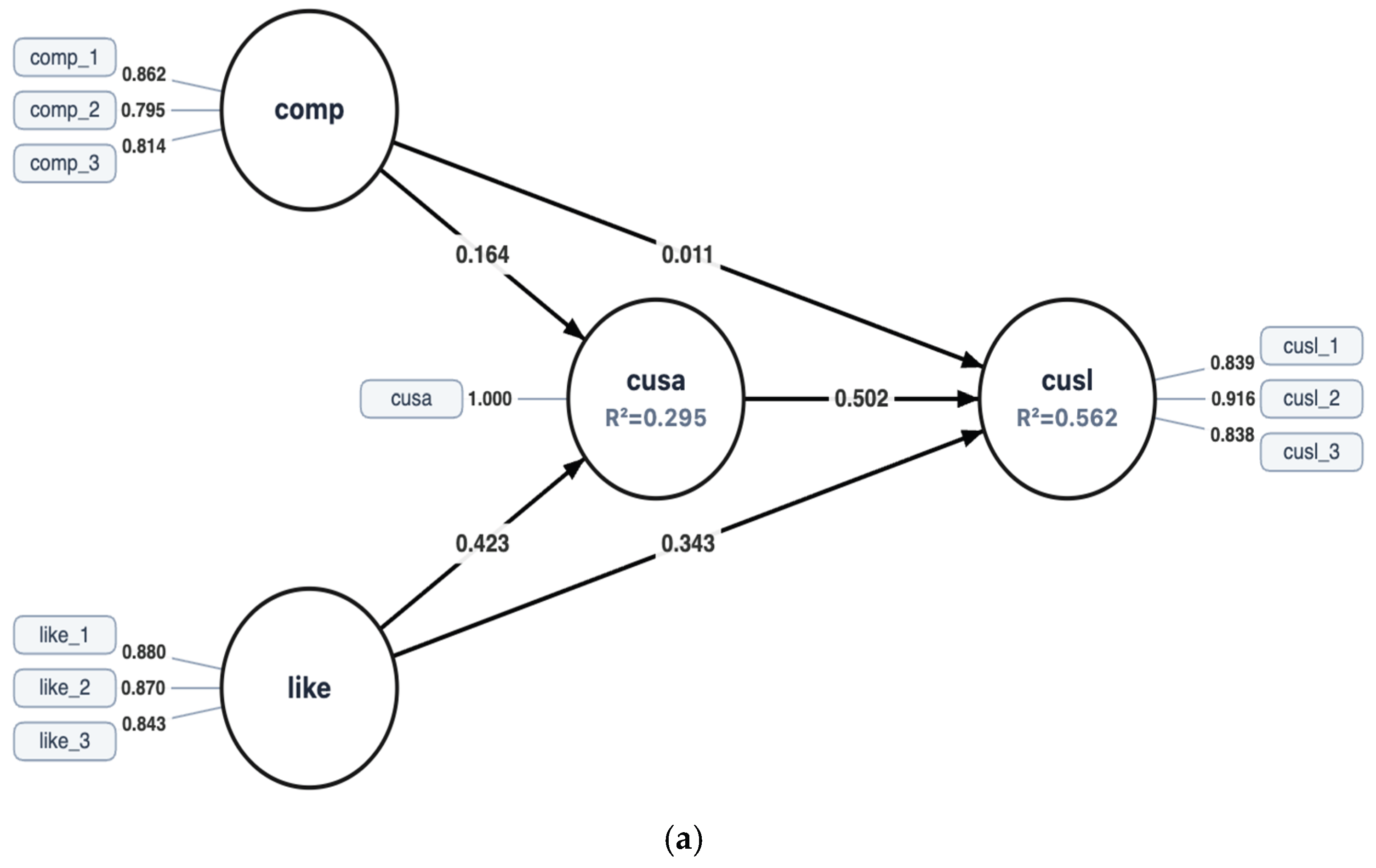
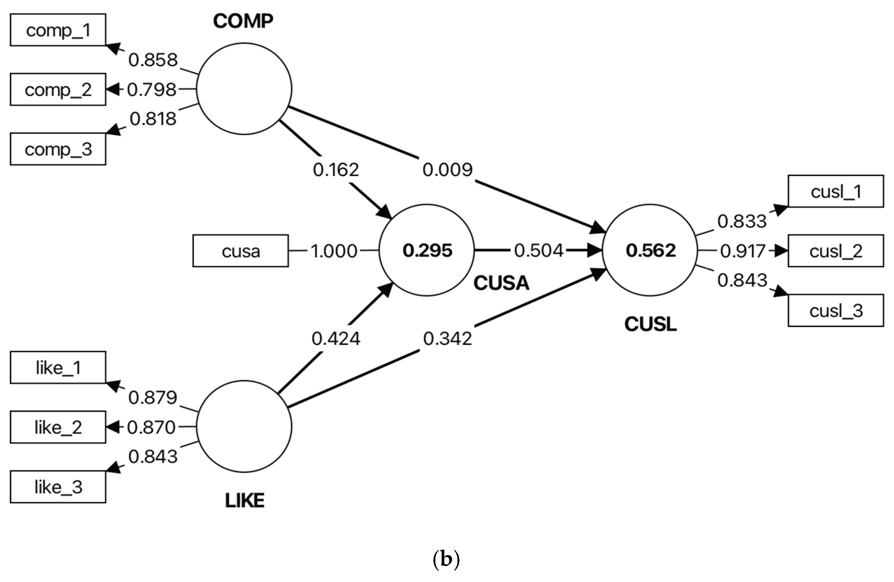
Figure 2.
Path model diagram for the Extended Moderation Model (Model 2) including the SWITCH × CUSA interaction term. (a) AnalyVa output. (b) SmartPLS 4 output.
Figure 2.
Path model diagram for the Extended Moderation Model (Model 2) including the SWITCH × CUSA interaction term. (a) AnalyVa output. (b) SmartPLS 4 output.
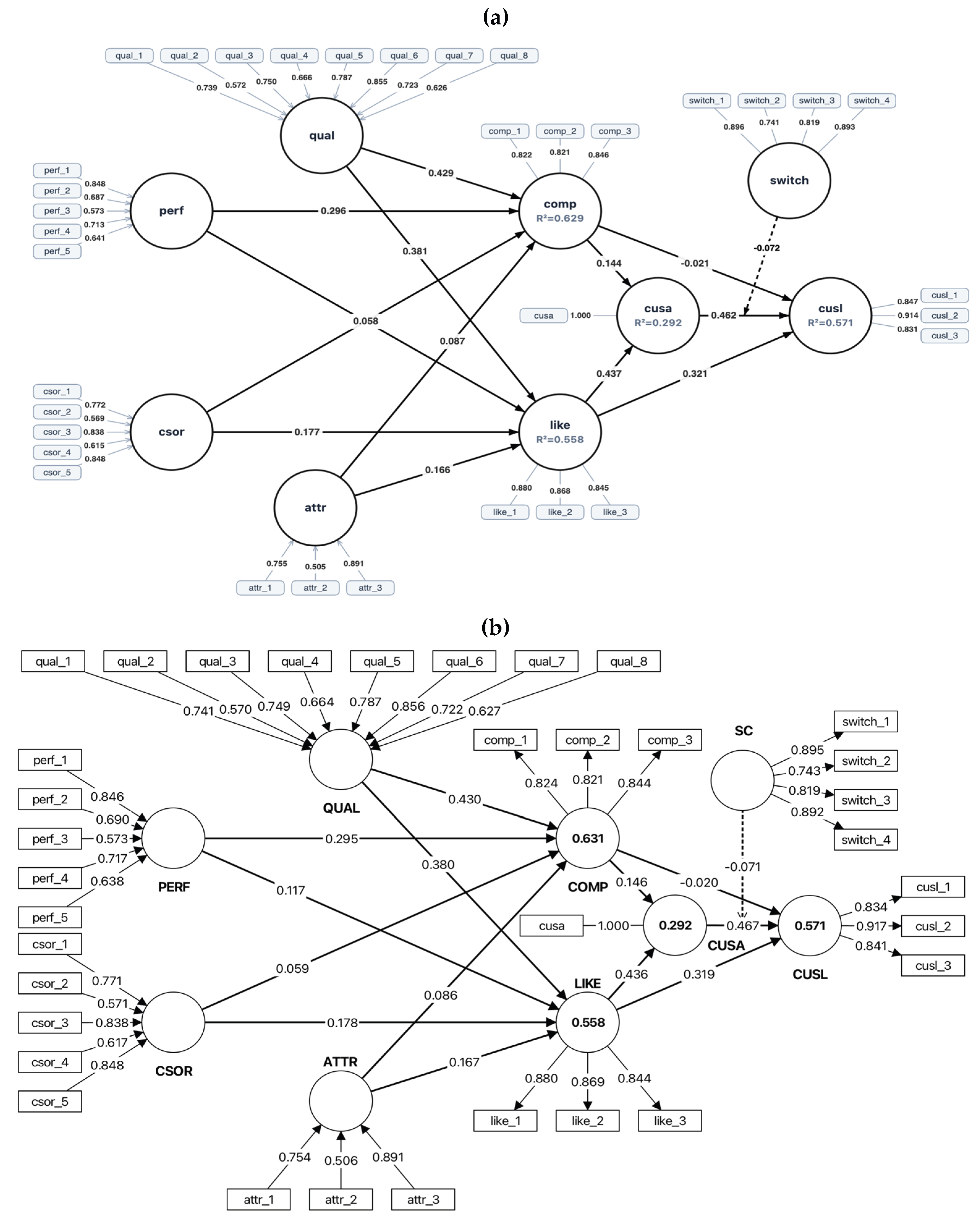
Figure 3.
Path model diagram for the Multiple Interaction Model (Model 3) with three single-item moderators (SWITCH1, SWITCH2, SWITCH3) and LIKE as simultaneous moderators. (a) AnalyVa output. (b) SmartPLS 4 output.
Figure 3.
Path model diagram for the Multiple Interaction Model (Model 3) with three single-item moderators (SWITCH1, SWITCH2, SWITCH3) and LIKE as simultaneous moderators. (a) AnalyVa output. (b) SmartPLS 4 output.
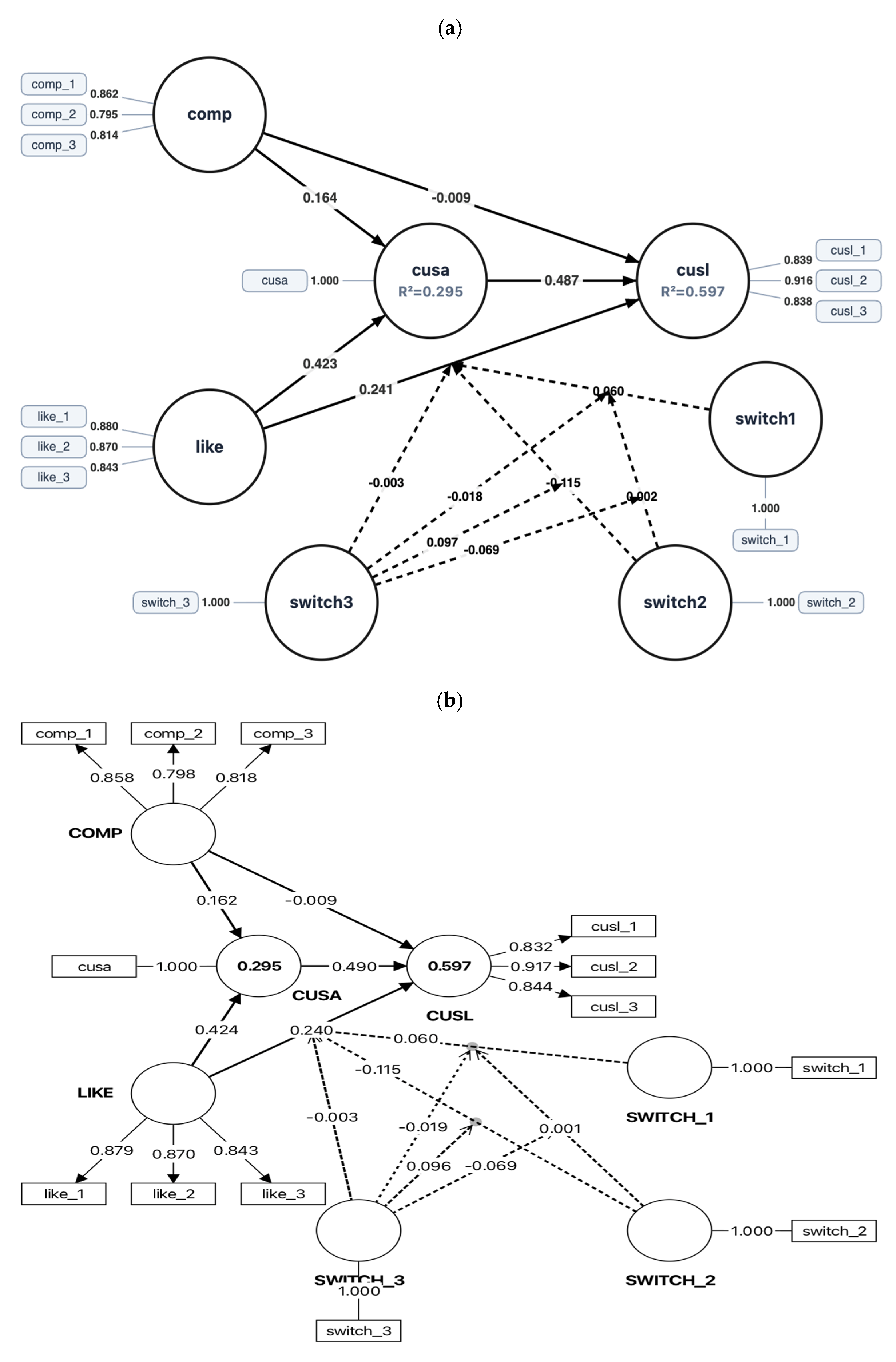

Table 1.
Outer Loadings for the Simple Reflective Model (Model 1): SmartPLS 4 versus AnalyVa.
| Construct | Indicator | SmartPLS | AnalyVa | |Δ| |
| COMP | comp_1 | .858 | .862 | .004 |
| comp_2 | .798 | .795 | .003 | |
| comp_3 | .818 | .814 | .004 | |
| CUSA | cusa | 1.000 | 1.000 | .000 |
| CUSL | cusl_1 | .833 | .839 | .006 |
| cusl_2 | .917 | .916 | .001 | |
| cusl_3 | .843 | .838 | .005 | |
| LIKE | like_1 | .879 | .880 | .001 |
| like_2 | .870 | .870 | .000 | |
| like_3 | .843 | .843 | .000 |
Note. |Δ| = absolute difference between platforms. All loadings meet the >.70 threshold in both platforms. CUSA is a single-item construct.
Table 2.
Construct Reliability and Validity for the Simple Reflective Model (Model 1): SmartPLS 4 versus AnalyVa.
Table 2.
Construct Reliability and Validity for the Simple Reflective Model (Model 1): SmartPLS 4 versus AnalyVa.
| SmartPLS α | AnalyVa α | SmartPLS ρa | AnalyVa ρa | SmartPLS ρc | AnalyVa ρc | SmartPLS AVE | AnalyVa AVE | |
| COMP | .776 | .776 | .832 | .847 | .865 | .864 | .681 | .679 |
| CUSL | .831 | .831 | .839 | .891 | .899 | .899 | .748 | .748 |
| LIKE | .831 | .831 | .836 | .888 | .899 | .899 | .747 | .747 |
Note. α = Cronbach’s alpha; ρa = Dijkstra-Henseler reliability (rho_a; Dijkstra & Henseler, 2015); ρc = composite reliability (rho_c); AVE = average variance extracted. All values meet recommended thresholds (α, ρa, ρc > .70; AVE > .50).
Table 3.
HTMT Discriminant Validity Ratios for the Simple Reflective Model (Model 1): SmartPLS 4 versus AnalyVa.
Table 3.
HTMT Discriminant Validity Ratios for the Simple Reflective Model (Model 1): SmartPLS 4 versus AnalyVa.
| Construct Pair | SmartPLS HTMT | AnalyVa HTMT | |Δ| |
| COMP—CUSA | .465 | .466 | .001 |
| COMP—CUSL | .532 | .533 | .001 |
| COMP—LIKE | .780 | .780 | .000 |
| CUSA—CUSL | .755 | .755 | .000 |
| CUSA—LIKE | .577 | .577 | .000 |
| CUSL—LIKE | .737 | .737 | .000 |
Note. HTMT = heterotrait-monotrait ratio (Henseler et al., 2015). Values below .85 indicate satisfactory discriminant validity. |Δ| = absolute difference between platforms.
Table 4.
Structural Model Results for the Simple Reflective Model (Model 1): SmartPLS 4 versus AnalyVa.
Table 4.
Structural Model Results for the Simple Reflective Model (Model 1): SmartPLS 4 versus AnalyVa.
| Path / Index | SmartPLS | AnalyVa | |Δ| |
| --- Path Coefficients --- | |||
| COMP → CUSA | .162 | .164 | .002 |
| COMP → CUSL | .009 | .011 | .002 |
| CUSA → CUSL | .504 | .502 | .002 |
| LIKE → CUSA | .424 | .423 | .001 |
| LIKE → CUSL | .342 | .343 | .001 |
| --- Specific Indirect Effects --- | |||
| COMP → CUSA → CUSL | .082 | .082 | .000 |
| LIKE → CUSA → CUSL | .214 | .212 | .002 |
| --- R² --- | |||
| CUSA | .295 | .295 | .000 |
| CUSL | .562 | .562 | .000 |
| --- f² --- | |||
| COMP → CUSA | .022 | .022 | .000 |
| COMP → CUSL | .000 | .000 | .000 |
| CUSA → CUSL | .410 | .406 | .004 |
| LIKE → CUSA | .149 | .148 | .001 |
| LIKE → CUSL | .136 | .136 | .000 |
Note. β = standardized path coefficient. f² = effect size. R² = coefficient of determination. Rows beginning with “---” are section headers, not data rows. |Δ| = absolute difference.
Table 5.
Model Fit Indices Across All Three Model Specifications: SmartPLS 4 versus AnalyVa.
| Index | M1 SmartPLS | M1 AnalyVa | M2 SmartPLS | M2 AnalyVa | M3 SmartPLS | M3 AnalyVa |
| SRMR (saturated) | .074 | .074 | .063 | .067 | .063 | .041 |
| SRMR (estimated) | .074 | .103 | .064 | .075 | .065 | .052 |
| NFI (saturated) | .820 | .818 | .605 | .559 | .848 | .933 |
| NFI (estimated) | .820 | .758 | .606 | .542 | .860 | .914 |
Note. M1 = Simple Reflective Model; M2 = Extended Moderation Model; M3 = Multiple Interaction Model. SRMR = standardized root mean square residual (threshold ≤ .08). NFI = normed fit index (threshold ≥ .90). Saturated = all possible paths freely estimated; Estimated = hypothesized paths only.
Table 6.
Structural Path Coefficients for the Extended Moderation Model (Model 2): SmartPLS 4 versus AnalyVa.
Table 6.
Structural Path Coefficients for the Extended Moderation Model (Model 2): SmartPLS 4 versus AnalyVa.
| Path | SmartPLS β | AnalyVa β | |Δ| |
| --- Core Model --- | |||
| COMP → CUSA | .146 | .144 | .002 |
| COMP → CUSL | −.020 | −.021 | .001 |
| CUSA → CUSL | .467 | .462 | .005 |
| LIKE → CUSA | .436 | .437 | .001 |
| LIKE → CUSL | .319 | .321 | .002 |
| --- Moderation --- | |||
| SWITCH → CUSL (main effect) | .070 | .075 | .005 |
| SWITCH × CUSA → CUSL | −.071 | −.072 | .001 |
| --- Antecedents to COMP --- | |||
| QUAL → COMP | .430 | .429 | .001 |
| PERF → COMP | .295 | .296 | .001 |
| CSOR → COMP | .059 | .058 | .001 |
| ATTR → COMP | .086 | .087 | .001 |
| --- Antecedents to LIKE --- | |||
| QUAL → LIKE | .380 | .381 | .001 |
| PERF → LIKE | .117 | .118 | .001 |
| CSOR → LIKE | .178 | .177 | .001 |
| ATTR → LIKE | .167 | .166 | .001 |
| --- R² --- | |||
| COMP | .631 | .629 | .002 |
| CUSA | .292 | .292 | .000 |
| CUSL | .571 | .571 | .000 |
| LIKE | .558 | .558 | .000 |
Note. β = standardized path coefficient. SWITCH = Switching Barriers (composite). SWITCH × CUSA = interaction term. Rows beginning with “---” are section headers. |Δ| = absolute difference.
Table 7.
Structural Path Coefficients for the Multiple Interaction Model (Model 3): SmartPLS 4 versus AnalyVa.
Table 7.
Structural Path Coefficients for the Multiple Interaction Model (Model 3): SmartPLS 4 versus AnalyVa.
| Path. | SmartPLS β | AnalyVa β | |Δ| |
| --- Main Effects on CUSA --- | |||
| COMP → CUSA | .162 | .162 | .000 |
| LIKE → CUSA | .424 | .424 | .000 |
| --- Main Effects on CUSL --- | |||
| COMP → CUSL | −.009 | −.010 | .001 |
| CUSA → CUSL | .490 | .484 | .006 |
| LIKE → CUSL | .240 | .242 | .002 |
| SWITCH1 → CUSL | .052 | .061 | .009 |
| SWITCH2 → CUSL | .085 | .082 | .003 |
| SWITCH3 → CUSL | −.021 | −.021 | .000 |
| --- Two-Way Interactions on CUSL --- | |||
| SWITCH1 × LIKE → CUSL | .060 | .060 | .000 |
| SWITCH2 × LIKE → CUSL | −.115 | −.114 | .001 |
| SWITCH3 × LIKE → CUSL | −.003 | −.004 | .001 |
| SWITCH2 × SWITCH1 → CUSL | .154 | .153 | .001 |
| SWITCH3 × SWITCH1 → CUSL | −.089 | −.096 | .007 |
| SWITCH3 × SWITCH2 → CUSL | .047 | .049 | .002 |
| --- Three-Way Interactions on CUSL --- | |||
| SWITCH3 × SWITCH2 × SWITCH1 → CUSL | −.106 | −.109 | .003 |
| SWITCH2 × SWITCH1 × LIKE → CUSL | .001 | .002 | .001 |
| SWITCH3 × SWITCH1 × LIKE → CUSL | −.019 | −.017 | .002 |
| SWITCH3 × SWITCH2 × LIKE → CUSL | .096 | .097 | .001 |
| --- Four-Way Interaction on CUSL --- | |||
| SWITCH3 × SWITCH2 × SWITCH1 × LIKE → CUSL | −.069 | −.069 | .000 |
| --- R² --- | |||
| CUSA | .295 | .295 | .000 |
| CUSL | .597 | .597 | .000 |
Note. β = standardized path coefficient. SWITCH1, SWITCH2, SWITCH3 = single-item switching barrier constructs. “×” denotes product interaction terms. |Δ| = absolute difference.
Disclaimer/Publisher’s Note: The statements, opinions and data contained in all publications are solely those of the individual author(s) and contributor(s) and not of MDPI and/or the editor(s). MDPI and/or the editor(s) disclaim responsibility for any injury to people or property resulting from any ideas, methods, instructions or products referred to in the content. |
© 2026 by the authors. Licensee MDPI, Basel, Switzerland. This article is an open access article distributed under the terms and conditions of the Creative Commons Attribution (CC BY) license (http://creativecommons.org/licenses/by/4.0/).
Copyright: This open access article is published under a Creative Commons CC BY 4.0 license, which permit the free download, distribution, and reuse, provided that the author and preprint are cited in any reuse.