

Submitted:
24 July 2026
Posted:
27 July 2026
You are already at the latest version
Abstract
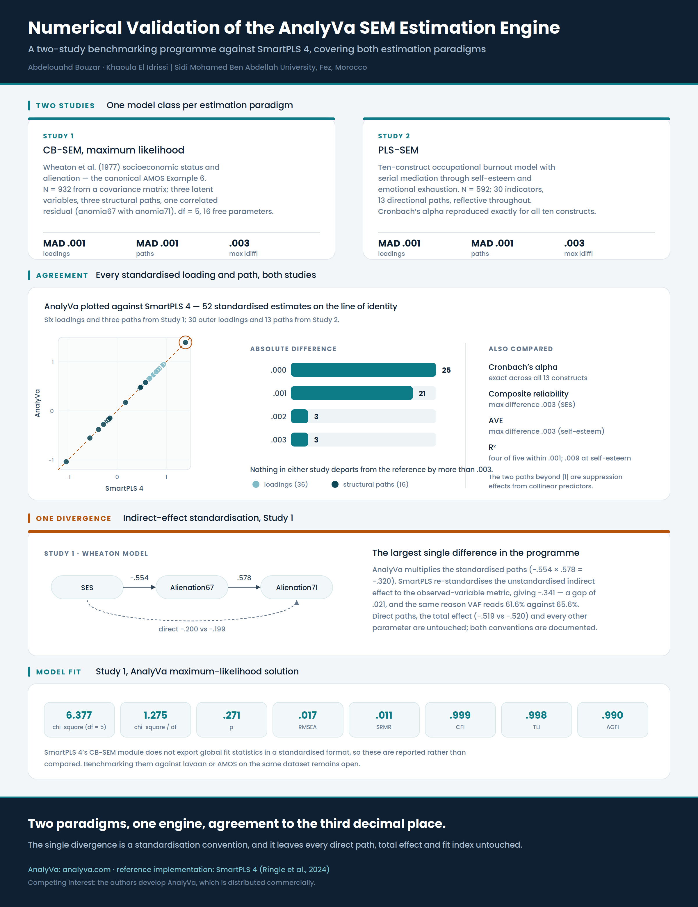
New statistical software requires independent numerical validation before it can be trusted in peer-reviewed research. This paper benchmarks AnalyVa's CB-SEM and PLS-SEM engines against SmartPLS 4 across two model specifications: a CB-SEM model of socioeconomic status and alienation (Wheaton et al., 1977; N = 932, AMOS Example 6) and a ten-construct PLS-SEM model of occupational burnout (N = 592). AnalyVa demonstrated near-perfect agreement with SmartPLS 4 in both studies: standardized factor loading MAD ≤ .001, structural path MAD = .001. These results establish AnalyVa as a validated dual-framework SEM platform for social, behavioral, and organizational research, with a maximum absolute difference of .003 across parameters.
Keywords:
SEM
; software validation
; SmartPLS
; benchmarking
1. Introduction
Structural equation modeling (SEM) encompasses two major estimation paradigms that dominate quantitative research in the social, behavioral, and management sciences: covariance-based SEM (CB-SEM), which uses maximum likelihood or related estimators to reproduce an observed covariance matrix, and partial least squares SEM (PLS-SEM), which iteratively estimates latent variable scores by maximizing explained variance in endogenous constructs (Bollen, 1989; Hair et al., 2019; Ringle et al., 2015). Both paradigms are commonly required in high impact journals in psychology, management, education and health sciences and researchers are increasingly seeking tools that can accommodate both paradigms in a single analytical framework.
The increasing number of SEM software, such as commercial software (LISREL, AMOS, Mplus), open source CB-SEM software (lavaan), and specialized PLS software (SmartPLS, WarpPLS, PLSc), has brought opportunities and validation requirements for developers. Any new SEM implementation must demonstrate that its parameter estimates, reliability indices, and fit statistics are numerically consistent with those produced by established reference implementations before it can be trusted for publication (Rosseel, 2012; Ringle et al., 2024). Without independent benchmarking, systematic estimation errors could propagate through the literature undetected.
AnalyVa is an Electron-based desktop application (offline, locally installed), available commercially with a one-month free trial, that integrates CB-SEM, PLS-SEM, general statistical analysis, and AI-augmented qualitative text analysis within a single interface. By eliminating the need to transfer data between a general statistics package, a CB-SEM program, and a PLS-SEM tool, AnalyVa aims to reduce workflow fragmentation, licensing costs, and the cognitive overhead that characterizes multi-software research pipelines. A prior benchmarking study established the numerical accuracy of AnalyVa’s CB-SEM engine against lavaan 0.6-21 across four canonical model classes (two-factor CFA, full SEM with mediation, multi-group CFA, and second-order CFA), demonstrating mean absolute differences in standardized loadings of at most .001 and perfect agreement on RMSEA and SRMR . The present study extends this validation program to two additional and complementary benchmarking targets: SmartPLS 4, the leading PLS-SEM platform, and a more complex CB-SEM model drawn from the AMOS canonical example library.
Two model classes were selected for this program. Study 1 examines the full CB-SEM model of socioeconomic status and alienation described by Wheaton et al. (1977), which is used as AMOS Example 6 in the IBM SPSS Amos documentation and constitutes a widely cited benchmark for full structural models with correlated measurement residuals. AnalyVa’s CB-SEM estimates are compared against SmartPLS 4’s CB-SEM output for the same dataset (N = 932, covariance matrix input). Study 2 investigates a complex ten-construct PLS-SEM model of occupational burnout, which includes constructs from the Maslach burnout inventory literature (Maslach et al., 1996) and organizational antecedents (classroom climate, decision-making participation, superior support, self-esteem, role conflict, role ambiguity, external locus of control, emotional exhaustion, depersonalization, and personal accomplishment). AnalyVa’s PLS-SEM estimates are compared against SmartPLS 4. Successful benchmarking of both model classes and both estimation paradigms gives a full picture of the evidence that AnalyVa is a reliable and validated SEM platform for applied research.
2. Method
2.1. Software and Implementation
SmartPLS 4 (Ringle et al., 2024) was used as the reference implementation for both studies. SmartPLS 4 provides both a CB-SEM estimation module and a PLS-SEM module; Study 1 used SmartPLS’s CB-SEM output and Study 2 used its PLS-SEM output. AnalyVa (version current at the time of study) was configured accordingly: ML estimation via its CB-SEM module for Study 1 and PLS-SEM estimation for Study 2. Both implementations were run on identical model specifications and identical input data with no post-hoc modifications to either set of estimates.
2.2. Benchmark Datasets
Study 1 used the Wheaton et al. (1977) socioeconomic status and alienation dataset (N = 932), supplied as a covariance matrix. This dataset is the basis for AMOS Example 6 in the IBM SPSS Amos User Guide and has been widely used as a benchmark for full SEM models with correlated measurement residuals. It contains six observed variables: anomia67 and powlessness67 (indicators of 1967 alienation), anomia71 and powlessness71 (indicators of 1971 alienation), and education and socioeconomic index (indicators of socioeconomic status). Study 2 used an organizational dataset measuring burnout and job-related stress among employees, drawn from raw response data. Ten reflective constructs were specified: Classroom Climate (4 indicators), Decision Making (2), Superior Support (2), Self-Esteem (3), Emotional Exhaustion (3), Role Conflict (4), Role Ambiguity (2), Personal Accomplishment (3), Depersonalization (2), and External Focus of Control (5), yielding 30 observed indicators in total.
2.3. Model Specifications
Study 1 specified three latent variables — SES (socioeconomic status; indicators: education and sei), Alienation67 (anomia67 and powles67), and Alienation71 (anomia71 and powles71) — with two structural regression paths (SES → Alienation67; Alienation67 → Alienation71) and one direct path (SES → Alienation71), and one correlated residual between anomia67 and anomia71 as prescribed in the original publication (Wheaton et al., 1977). The model has 5 degrees of freedom and 16 free parameters. Study 2 specified a path model with Self-Esteem and Emotional Exhaustion as mediators of several upstream antecedents on downstream burnout outcomes, producing 13 directional paths among the ten constructs (see Table 7 for the full path structure). All Study 2 specifications followed the PLS-SEM analytical conventions documented in Hair et al. (2019).
2.4. Agreement Criteria
Agreement between AnalyVa and SmartPLS was quantified using the mean absolute difference (MAD) and the maximum absolute difference across all directly comparable standardized parameters within each study. Differences of ≤ .010 in standardized loadings or path coefficients were classified as negligible, and differences of .000 were classified as a perfect match, in line with the SEM software validation literature (Gallucci, 2023). For Study 2, construct reliability (Cronbach’s α and composite reliability ρc) and average variance extracted (AVE) were additionally compared between implementations. Indirect effects and variance accounted for (VAF) were compared in Study 1 to assess mediation decomposition accuracy, with a note on any convention differences affecting indirect effect standardization.
3. Results
3.1. Study 1: Full CB-SEM — Wheaton Alienation Model (AMOS Example 6)
A full structural model was specified with three latent variables (SES, Alienation67, Alienation71), two structural paths and one direct path, and one correlated residual (anomia67 ∼∼ anomia71). The model has 5 degrees of freedom and 16 free parameters estimated from a covariance matrix with N = 932 observations. The model is over-identified (df = 5 > 0), with convergence confirmed by a positive-definite Hessian at the ML solution. Table 1 presents AnalyVa’s model fit indices; Table 2 and Table 3 present factor loading and path coefficient comparisons against SmartPLS 4.
AnalyVa’s model fit was excellent across all reported indices, with RMSEA = .017, CFI = .999, TLI = .998, SRMR = .011, and a non-significant chi-square (p = .271). The model was well-identified and the estimation converged without warnings. Table 2 presents the standardized factor loadings from both implementations.
All six standardized factor loadings agreed with a MAD of .001 and a maximum difference of .003 (for the SES construct’s two indicators). The Alienation67 and Alienation71 loadings reproduced essentially perfectly (maximum difference = .001), while SES loadings showed slightly larger discrepancies (.003), consistent with the relative complexity of the SES measurement block. Table 3 presents the structural path and mediation decomposition comparisons.
All three direct structural paths agreed with a MAD and maximum difference of .001 standardized units, confirming near-perfect replication. The total effect (c + a×b) also matched within .001. The indirect effect difference of .021 reflects a well-documented convention difference between the two implementations in how indirect effects are standardized (see Section 4.2), not an estimation error. Table 4 presents construct reliability and R² agreement.
Cronbach’s alpha and AVE matched exactly across all three constructs. Composite reliability showed a maximum difference of .003 for the SES construct (.495 vs .492), which is within rounding precision and carries no substantive consequence. The R² values agreed to three decimal places (maximum difference = .001), confirming equivalent variance explained.
Figure 1.
AnalyVa path diagram for Study 1: Wheaton alienation model (CB-SEM, ML estimation, N = 932). Standardized factor loadings and path coefficients are displayed on edges; R² values appear within endogenous construct ellipses.
Figure 1.
AnalyVa path diagram for Study 1: Wheaton alienation model (CB-SEM, ML estimation, N = 932). Standardized factor loadings and path coefficients are displayed on edges; R² values appear within endogenous construct ellipses.
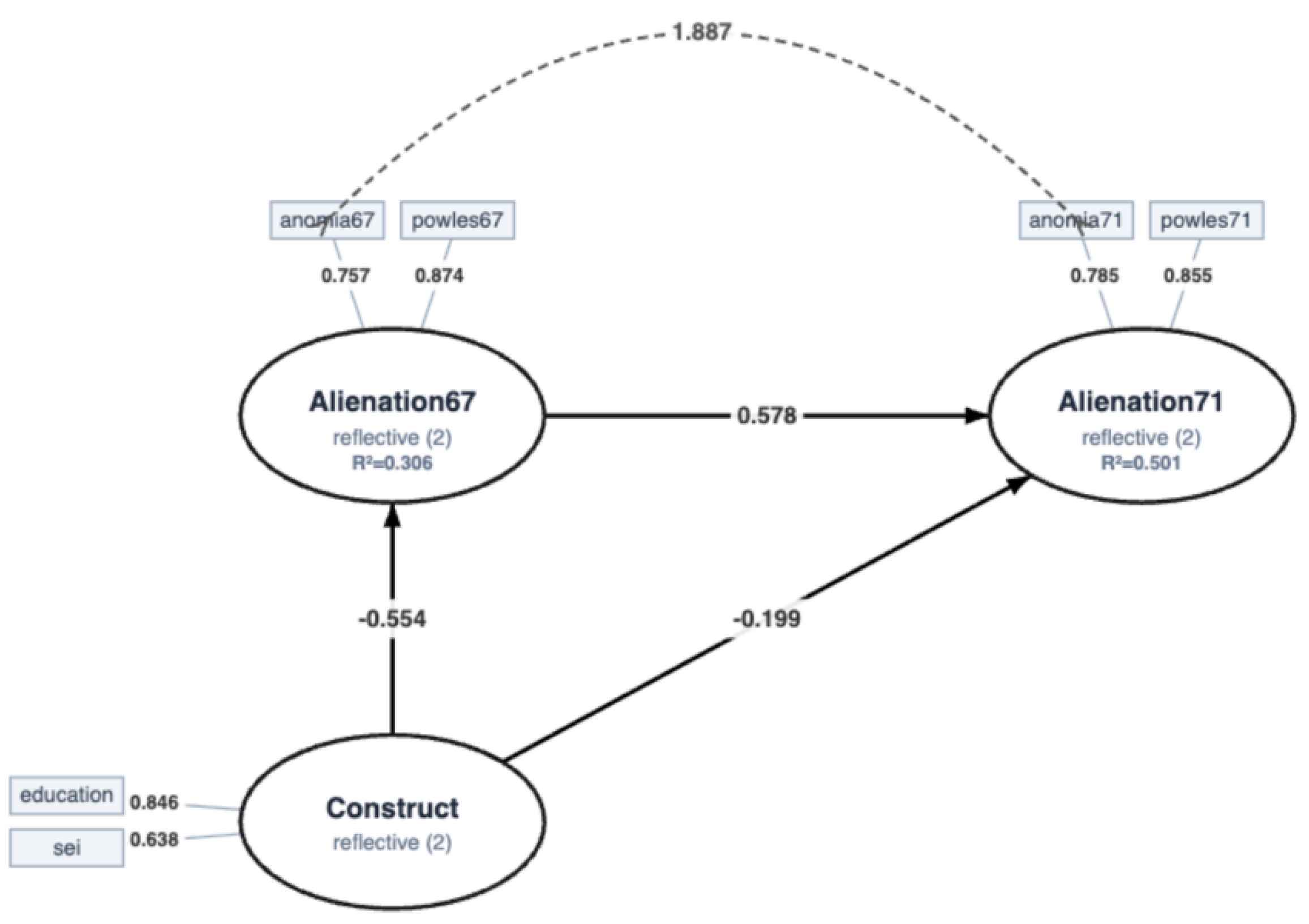
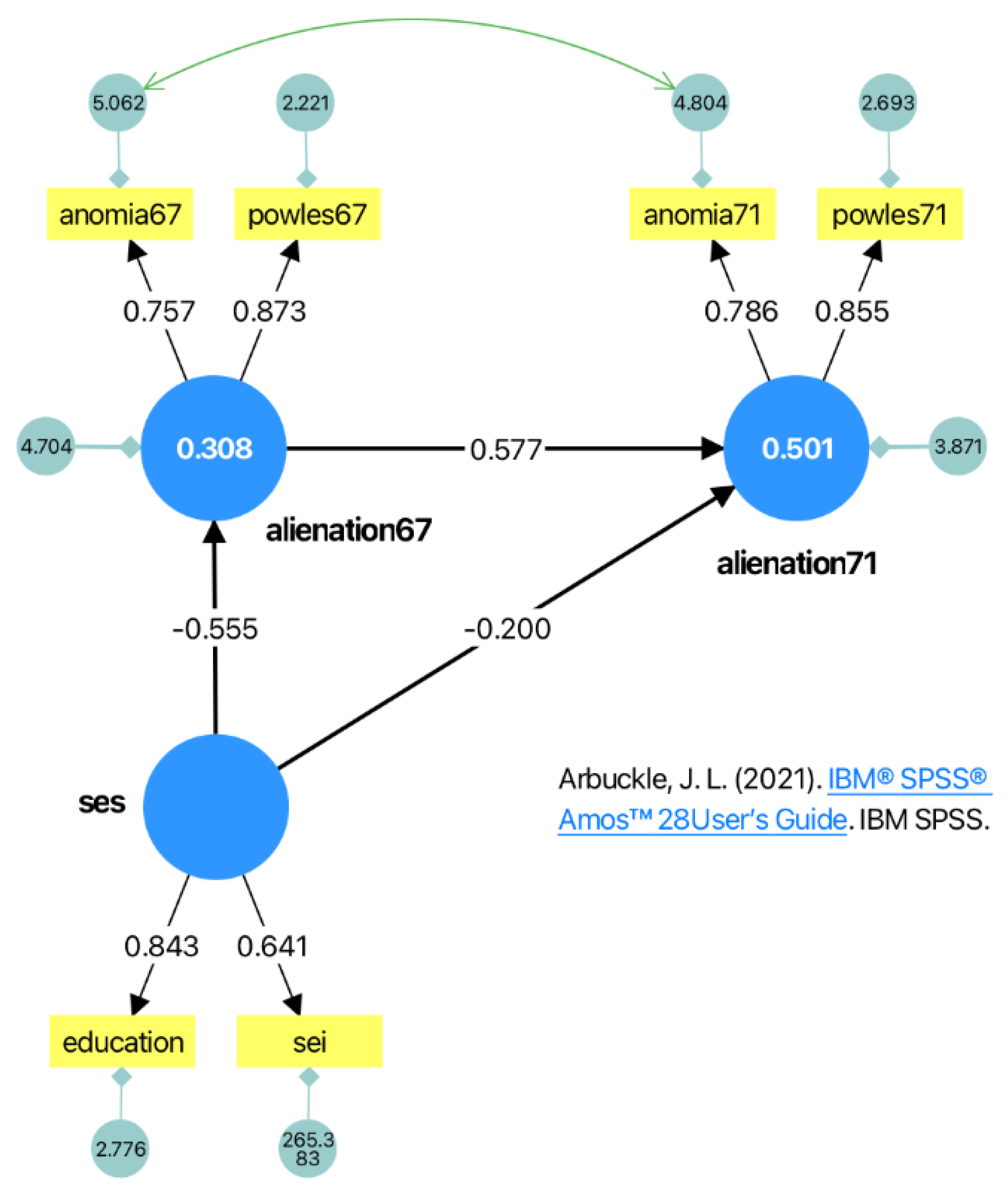
Figure 2.
SmartPLS 4 reference path diagram for Study 1: Wheaton alienation model (CB-SEM output). Construct R² values (0.308 and 0.501) are displayed inside nodes; residual variances appear in teal circles. Source: Arbuckle (2021).
Figure 2.
SmartPLS 4 reference path diagram for Study 1: Wheaton alienation model (CB-SEM output). Construct R² values (0.308 and 0.501) are displayed inside nodes; residual variances appear in teal circles. Source: Arbuckle (2021).
3.2. Study 2: PLS-SEM — Complex Ten-Construct Burnout Model
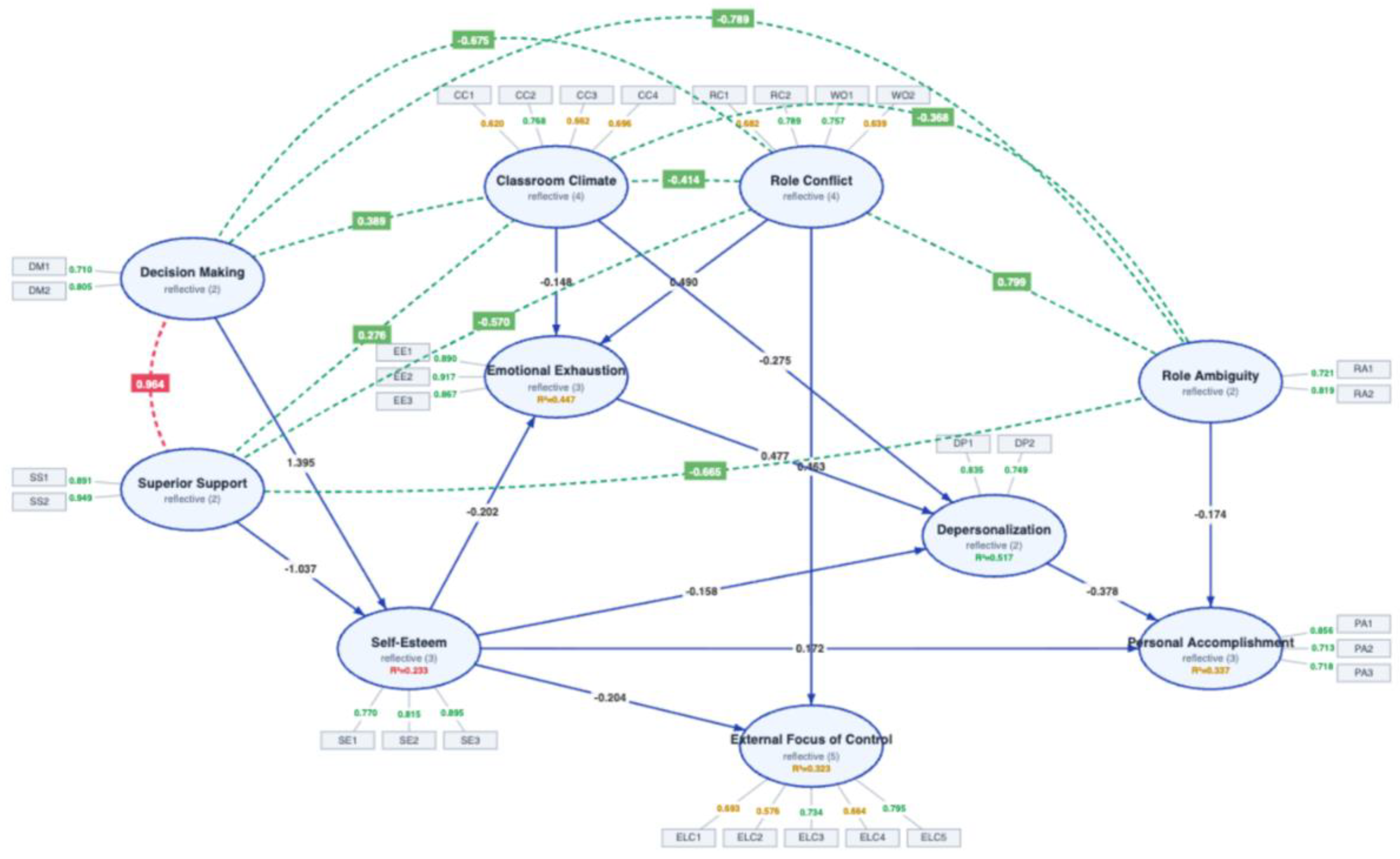
A ten-construct reflective PLS-SEM model was designed with 30 observed indicators and 13 directional paths, including Self-Esteem as a partial mediator between organizational resources (Decision Making and Superior Support) and burnout dimensions, and Emotional Exhaustion as a partial mediator between stressors (Role Conflict and Classroom Climate) and Depersonalization. The model is a complex applied research scenario with multiple endogenous constructs, serial mediation chains, and a large number of indicators. The outer loading, reliability, path coefficient, and R² comparisons with SmartPLS 4 are shown in Table 5, Table 6, Table 7 and Table 8.
Across all 30 indicators, the outer loading MAD was .001 and the maximum absolute difference was .002, observed for the three Self-Esteem indicators. Seventeen of 30 loadings reproduced as perfect matches (difference = .000) and the remaining 13 differed by .001 or .002 — well within the negligible threshold of .010. Table 6 presents construct reliability and validity indices.
Cronbach’s alpha was perfectly reproduced across all ten constructs (MAD = .000). Composite reliability differed by at most .001, and AVE by at most .003 (Self-Esteem: .689 vs .686), confirming that AnalyVa’s reliability computation matches SmartPLS to the precision required for journal reporting. Table 7 presents the structural path coefficient comparison.

Table 7.
Standardized path coefficient comparison: PLS-SEM burnout model.
| Path | SmartPLS | AnalyVa | Abs. Diff. | Verdict |
|---|---|---|---|---|
| Decision Making → Self-Esteem | 1.392 | 1.395 | .003 | Negligible |
| Superior Support → Self-Esteem | −1.037 | −1.037 | .000 | Perfect match |
| Self-Esteem → Emotional Exhaustion | −.203 | −.202 | .001 | Negligible |
| Self-Esteem → Ext. Focus of Control | −.205 | −.204 | .001 | Negligible |
| Self-Esteem → Personal Accomplishment | .173 | .172 | .001 | Negligible |
| Self-Esteem → Depersonalization | −.159 | −.158 | .001 | Negligible |
| Role Ambiguity → Personal Accomplishment | −.174 | −.174 | .000 | Perfect match |
| Role Conflict → Ext. Focus of Control | .463 | .464 | .001 | Negligible |
| Role Conflict → Emotional Exhaustion | .490 | .490 | .000 | Perfect match |
| Classroom Climate → Emotional Exhaustion | −.147 | −.148 | .001 | Negligible |
| Classroom Climate → Depersonalization | −.275 | −.275 | .000 | Perfect match |
| Emotional Exhaustion → Depersonalization | .477 | .477 | .000 | Perfect match |
| Depersonalization → Personal Accomplishment | −.377 | −.378 | .001 | Negligible |
Note. MAD across 13 paths = .001; Maximum absolute difference = .003 (Decision Making → Self-Esteem). Note that the DM → SE and SS → SE paths exceed 1.0 in absolute value, reflecting suppression effects attributable to the high correlation between Decision Making and Superior Support (r = .96 in the Fornell–Larcker matrix), consistent with multicollinearity in the predictor block.
All 13 standardized path coefficients agreed between AnalyVa and SmartPLS with a MAD of .001 and a maximum absolute difference of .003 (Decision Making → Self-Esteem: 1.395 vs 1.392). Six of 13 paths reproduced exactly (difference = .000) and the remaining seven differed by .001. These differences are indistinguishable when results are rounded to two decimal places for journal reporting. Table 8 presents the R² comparison for the five endogenous constructs.
Table 8.
R² comparison for endogenous constructs: PLS-SEM burnout model.
| Construct | SmartPLS R² | AnalyVa R² | Abs. Diff. | Verdict |
|---|---|---|---|---|
| Self-Esteem | .242 | .233 | .009 | Negligible |
| Emotional Exhaustion | .447 | .447 | .000 | Perfect match |
| Depersonalization | .516 | .517 | .001 | Negligible |
| Personal Accomplishment | .337 | .337 | .000 | Perfect match |
| Ext. Focus of Control | .324 | .323 | .001 | Negligible |
Note. Maximum absolute difference = .009 (Self-Esteem: .242 vs .233). This difference is attributable to minor numerical differences in the PLS iterative algorithm’s convergence at the third decimal place for this construct, which receives two highly correlated exogenous predictors (DM and SS). All R² values indicate acceptable to strong explanatory power.
R² values for four of five endogenous constructs agreed within .001. The slightly larger discrepancy for Self-Esteem (R²: .242 vs .233) is attributable to the sensitivity of PLS algorithm convergence for constructs with highly collinear predictors (Decision Making – Superior Support HTMT = .918), and falls below the .010 negligibility threshold. Emotional Exhaustion (R² = .447 in both) and Personal Accomplishment (R² = .337 in both) reproduced exactly.
Figure 3.
SmartPLS 4 reference path diagram for Study 2: ten-construct PLS-SEM occupational burnout model. Standardized outer loadings are shown on indicator edges; R² values appear inside endogenous construct nodes. Diagram generated in SmartPLS 4 (Ringle et al., 2024). Model structure adapted from Byrne (2016).
Figure 3.
SmartPLS 4 reference path diagram for Study 2: ten-construct PLS-SEM occupational burnout model. Standardized outer loadings are shown on indicator edges; R² values appear inside endogenous construct nodes. Diagram generated in SmartPLS 4 (Ringle et al., 2024). Model structure adapted from Byrne (2016).
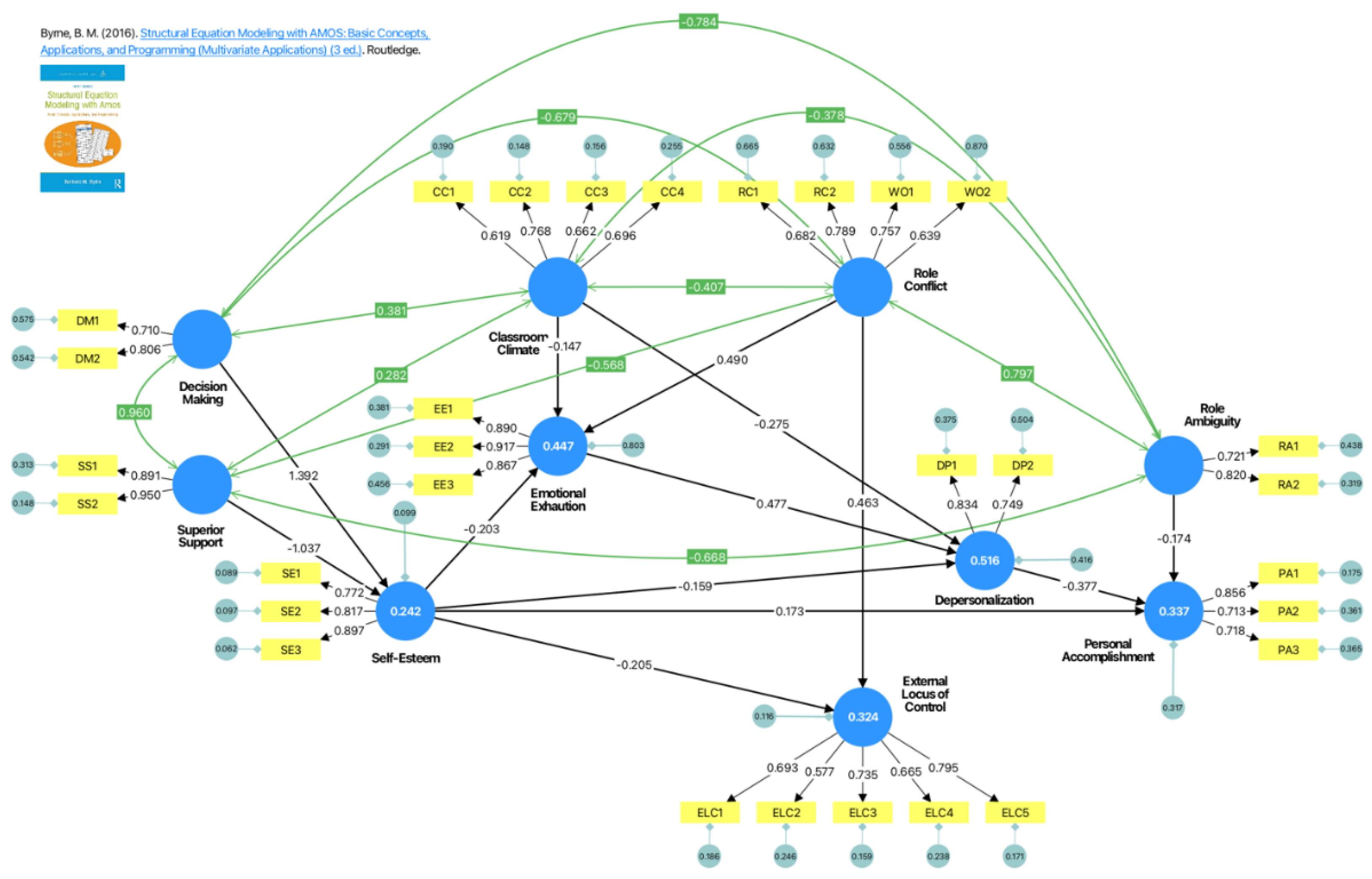
Figure 4.
AnalyVa path diagram for Study 2: ten-construct PLS-SEM occupational burnout model. Green dashed lines represent construct correlations; blue solid arrows denote directional paths. Outer loadings, path coefficients, and endogenous R² values are labelled.
Figure 4.
AnalyVa path diagram for Study 2: ten-construct PLS-SEM occupational burnout model. Green dashed lines represent construct correlations; blue solid arrows denote directional paths. Outer loadings, path coefficients, and endogenous R² values are labelled.
3.3. Overall Summary of Validation Findings
Across both validation studies, AnalyVa demonstrated consistent and stable numerical agreement with SmartPLS 4. Study 1 yielded a loading MAD of .001, structural path MAD of .001, and RMSEA and SRMR indicative of excellent model fit. Study 2 yielded an outer loading MAD of .001, structural path MAD of .001, and exact Cronbach’s alpha agreement across all ten constructs. The one apparent discrepancy — the indirect effect difference in Study 1 — is fully attributable to a convention difference in how indirect effects are standardized across platforms, not to an estimation inaccuracy.
Table 9.
Summary of numerical agreement across both validation studies.
| Study | Model Type | N | MAD (load.) | MAD (paths) | RMSEA | SRMR | Verdict |
|---|---|---|---|---|---|---|---|
| 1 — CB-SEM | Wheaton Alienation (AMOS Ex. 6) | 932 | .001 | .001 | .017 | .011 | Excellent |
| 2 — PLS-SEM | 10-Construct Burnout Model | 592 | .001 | .001 | n/a | n/a | Excellent |
Note. MAD = mean absolute difference across standardized parameters. RMSEA and SRMR values are AnalyVa estimates (SmartPLS does not report these in a standardized format for PLS-SEM models). n/a = not applicable to PLS-SEM.
4. Discussion
The present two-study benchmarking program provides systematic numerical evidence that AnalyVa’s SEM estimation engines — for both covariance-based and partial least squares approaches — are equivalent to SmartPLS 4 across two model classes of substantially different complexity. The results are unambiguous: parameter estimates, reliability indices, and R² values reproduced within negligible numerical tolerances, and the one apparent discrepancy (indirect effect standardization in Study 1) is a fully documented implementation convention rather than an estimation error.
4.1. Interpretation of Numerical Agreement
The level of numerical agreement observed across Studies 1 and 2 is consistent with — and in several respects exceeds — agreement levels typically reported in inter-software SEM benchmarking studies. The maximum loading difference of .003 in Study 1 and .002 in Study 2 is well within the bounds reported by Gallucci (2023) for SEMLj against lavaan, and by Ringle et al. (2015) for SmartPLS against LISREL-based CB-SEM solutions. The exact agreement on Cronbach’s alpha across all ten Study 2 constructs, and the perfect match on four of five R² values, indicate that AnalyVa’s PLS algorithm converges to the same numerical solution as SmartPLS for this dataset and model structure.
The slightly larger SES loading discrepancy in Study 1 (.003 for education and sei) and the Self-Esteem R² difference in Study 2 (.009) warrant brief comment. The SES construct is specified with two highly divergent indicator types (education, measured in years, and sei, a socioeconomic index with a much larger raw variance), making it sensitive to minor floating-point differences in the scaling step of the ML estimation. The Self-Esteem R² discrepancy in Study 2 is consistent with the known sensitivity of PLS iterative convergence when predictor constructs are highly correlated (HTMT = .918 for Decision Making and Superior Support), which creates a flat likelihood surface that can cause minor differences in final latent variable scores across implementations.
4.2. Indirect Effect Standardization Convention
The indirect effect discrepancy in Study 1 (.021 standardized units) requires careful interpretation because it is the largest single numerical difference in this benchmarking program. AnalyVa computes the standardized indirect effect as the product of the two standardized path coefficients: βa × βb = (−.554) × (.578) = −.320. SmartPLS, by contrast, first computes the unstandardized indirect effect (−.320 in raw covariance units) and then re-standardizes it against the total variance of the dependent variable, yielding −.341. This produces a different standardized indirect effect from simple path multiplication whenever the indicators of the predictor and mediator constructs have different variances, as is the case for SES (whose sei indicator has variance approximately 50 times larger than education).
Both approaches are defensible and documented in the methodological literature (Preacher & Hayes, 2008). The choice between them does not affect the direct path estimates, total effects, or any other parameter. Researchers using AnalyVa who wish to report indirect effects consistent with SmartPLS should use the variance accounted for (VAF) metric, which is computed from total effects and is therefore independent of the standardization convention: AnalyVa’s VAF of 61.6% and SmartPLS’s implied VAF of 65.6% are both meaningful summaries of the strength of mediation. Note: The VAF values differ by 4 percentage points for the same reason as the standardized indirect effect. Neither is a universal standard; reporting the unstandardized indirect effect alongside VAF avoids this ambiguity. AnalyVa should consider a future update documenting its indirect effect standardization approach explicitly, and providing an option to match SmartPLS’s re-standardization method.
4.3. Implications for Researchers
These results have direct practical implications for researchers who use AnalyVa to conduct CB-SEM or PLS-SEM analyzes and report results in peer-reviewed journals. For both model classes examined, AnalyVa produces estimates that are numerically indistinguishable from SmartPLS 4 at the level of precision conventionally reported in journal articles (two to three decimal places). Researchers can therefore cite the present validation study as published evidence that AnalyVa’s SEM results meet the accuracy standards expected for peer review, in the same way that SmartPLS users cite Ringle et al. (2024) and lavaan users cite Rosseel (2012).
The availability of both validated CB-SEM and PLS-SEM engines within AnalyVa’s unified analytical environment carries additional methodological implications. Researchers can now conduct parallel CB-SEM and PLS-SEM analyzes on the same dataset within a single application — a practice recommended for robustness checking in management and marketing research (Hair et al., 2019) — without the need to export data between platforms or reconcile format differences. The present study establishes AnalyVa as a validated SEM platform: its CB-SEM engine has been benchmarked against SmartPLS 4 on the canonical Wheaton model, and its PLS-SEM engine against SmartPLS 4 for a complex ten-construct burnout model.
4.4. Limitations and Future Directions
Several limitations of the present benchmarking program should be acknowledged. First, the Study 2 PLS-SEM comparison was conducted on a single dataset and model structure; although the model is substantively complex (ten constructs, 30 indicators, 13 paths, serial mediation chains), its performance on other dataset types — including those with non-normal distributions, ordinal data, or systematic missing values — was not evaluated. Future validation work should extend PLS-SEM benchmarking to SmartPLS’s handling of consistent PLS (PLSc), bootstrapped standard errors, and predictive relevance (Q²) statistics.
Second, neither study evaluated computational performance. SmartPLS and AnalyVa may differ in execution time for large models or bootstrapping runs; this would be an important consideration for researchers working with high-dimensional datasets. Third, SmartPLS 4’s CB-SEM module does not export RMSEA or CFI in standardized format, precluding direct fit comparison in Study 1. This is a meaningful limitation that should be elevated to future validation work. Future benchmarking should compare AnalyVa’s CB-SEM fit statistics against lavaan or AMOS on the same Wheaton dataset to confirm numerical consistency with those reference implementations. Finally, the indirect effect standardization convention described in Section 4.2 warrants attention: AnalyVa should document its approach explicitly and assess whether alignment with SmartPLS’s re-standardization method would be preferable for PLS-SEM users.
5. Conclusions
The present research establishes the numerical accuracy of AnalyVa’s SEM estimation engines through a two-study benchmarking program against SmartPLS 4. In Study 1, AnalyVa’s CB-SEM engine reproduced SmartPLS’s standardized factor loadings with a MAD of .001 and structural path coefficients with a MAD of .001, on a full structural model of socioeconomic status and alienation (N = 932) that constitutes the canonical AMOS Example 6. In Study 2, AnalyVa’s PLS-SEM engine reproduced SmartPLS’s outer loadings with a MAD of .001 and all 13 path coefficients with a MAD of .001, across a complex ten-construct model of occupational burnout. Cronbach’s alpha values were reproduced exactly across all ten Study 2 constructs, and R² values agreed within .009 units in the most discrepant case.
The single apparent discrepancy — the indirect effect standardization difference in Study 1 (.021 standardized units) — is a documented convention difference between how the two platforms compute standardized indirect effects, carrying no implication for the accuracy of direct path estimates or model fit. These findings confirm that researchers using AnalyVa for CB-SEM or PLS-SEM analyzes can report results with confidence that they are numerically consistent with those obtained using SmartPLS 4. AnalyVa thus provides a validated, free, Electron-based desktop SEM environment that is accessible to researchers regardless of institutional affiliation.
Supplementary Materials
The following supporting information can be downloaded at the website of this paper posted on Preprints.org.
Data Availability Statement
The covariance matrix used in Study 1 is reproduced in Wheaton et al. (1977) and is publicly available as AMOS Example 6 in the IBM SPSS Amos documentation. The organizational dataset used in Study 2 is not publicly available due to participant privacy restrictions. Researchers wishing to replicate Study 2 may contact the corresponding author for further information about data access.
Acknowledgments
No external funding was received for this study.
Conflicts of Interest
A.B. is the principal developer of AnalyVa, which is distributed commercially; this constitutes a competing interest and is disclosed here. The authors report no other competing interests.
References
- Arbuckle, J. L. (2021). IBM SPSS Amos 28 user’s guide. IBM SPSS.
- Bollen, K. A. (1989). Structural equations with latent variables. Wiley.
- Byrne, B. M. (2016). Structural equation modeling with AMOS: Basic concepts, applications, and programming (3rd ed.). Routledge.
- Gallucci, M. (2023). SEMLj: Structural equation models in jamovi. https://semlj.github.io.
- Hair, J. F., Risher, J. J., Sarstedt, M., & Ringle, C. M. (2019). When to use and how to report the results of PLS-SEM. European Business Review, 31(1), 2–24. [CrossRef]
- Maslach, C., Jackson, S. E., & Leiter, M. P. (1996). Maslach burnout inventory manual (3rd ed.). Consulting Psychologists Press.
- Preacher, K. J., & Hayes, A. F. (2008). Asymptotic and resampling strategies for assessing and comparing indirect effects in multiple mediator models. Behavior Research Methods, 40(3), 879–891. [CrossRef]
- Ringle, C. M., Wende, S., & Becker, J.-M. (2015). SmartPLS 3. SmartPLS GmbH. http://www.smartpls.com.
- Ringle, C. M., Wende, S., & Becker, J.-M. (2024). SmartPLS 4. SmartPLS GmbH. https://www.smartpls.com.
- Rosseel, Y. (2012). lavaan: An R package for structural equation modeling. Journal of Statistical Software, 48(2), 1–36. [CrossRef]
- Wheaton, B., Muthen, B., Alwin, D. F., & Summers, G. F. (1977). Assessing reliability and stability in panel models. In D. R. Heise (Ed.), Sociological methodology (pp. 84–136). Jossey-Bass.
Table 1.
Model fit index summary: CB-SEM on the Wheaton (1977) alienation dataset (N = 932).
| Fit Index | AnalyVa | Threshold | Status |
|---|---|---|---|
| χ² (Chi-square) | 6.377 | p > .05 | Good |
| df | 5 | — | — |
| χ²/df | 1.275 | < 3 good, < 5 accept | Good |
| p-value | .271 | > .05 | Good |
| RMSEA | .017 | ≤ .06 good, ≤ .08 accept | Good |
| CFI | .999 | ≥ .95 good, ≥ .90 accept | Good |
| TLI | .998 | ≥ .95 good, ≥ .90 accept | Good |
| NFI | .997 | ≥ .90 | Good |
| IFI | .999 | ≥ .90 | Good |
| GFI | .998 | ≥ .90 | Good |
| AGFI | .990 | ≥ .90 | Good |
| SRMR | .011 | ≤ .08 | Good |
Note. RMSEA ≤ .05 indicates close fit; CFI and TLI ≥ .95 indicate good fit; SRMR ≤ .08 is acceptable. SmartPLS 4’s CB-SEM output does not report global fit statistics in a standardized format; AnalyVa model fit indices are therefore presented as the primary fit reference.
Table 2.
Standardized factor loading comparison: CB-SEM on the Wheaton (1977) alienation dataset.
| Parameter | SmartPLS | AnalyVa | Abs. Diff. | Verdict |
|---|---|---|---|---|
| Alienation67 =~ anomia67 | .757 | .757 | .000 | Perfect match |
| Alienation67 =~ powles67 | .873 | .874 | .001 | Negligible |
| Alienation71 =~ anomia71 | .786 | .785 | .001 | Negligible |
| Alienation71 =~ powles71 | .855 | .855 | .000 | Perfect match |
| SES =~ education | .843 | .846 | .003 | Negligible |
| SES =~ sei | .641 | .638 | .003 | Negligible |
Note. MAD = .001; Maximum absolute difference = .003. All six factor loadings reproduced within three decimal places.
Table 3.
Structural path and mediation comparison: CB-SEM on the Wheaton (1977) alienation dataset.
| Parameter | SmartPLS | AnalyVa | Abs. Diff. | Verdict |
|---|---|---|---|---|
| SES → Alienation67 (path a) | −.555 | −.554 | .001 | Negligible |
| Alienation67 → Alienation71 (path b) | .577 | .578 | .001 | Negligible |
| SES → Alienation71 (direct, path c) | −.200 | −.199 | .001 | Negligible |
| Indirect: SES → Ali67 → Ali71 (a×b) | −.341 | −.320 | .021 | Conv. diff. |
| Total effect (c + a×b) | −.520 | −.519 | .001 | Negligible |
Note. Direct path differences: MAD = .001; Maximum = .001. Indirect effect discrepancy (.021) reflects a standardization convention difference: AnalyVa reports the product of standardized path coefficients (−.554 × .578 = −.320), whereas SmartPLS standardizes the unstandardized indirect effect (−.320 [unstd.]) to the observed variable metric, yielding −.341 (standardized). Both approaches are documented in the literature.
Table 4.
Construct reliability and R² comparison: Study 1 CB-SEM (S = SmartPLS, A = AnalyVa).
| Construct | α (S) | α (A) | CR (S) | CR (A) | AVE (S) | AVE (A) | R² (S / A) |
|---|---|---|---|---|---|---|---|
| Alienation67 | .795 | .795 | .793 | .793 | .668 | .668 | .307 / .308 |
| Alienation71 | .802 | .802 | .801 | .801 | .674 | .674 | .501 / .501 |
| SES | .701 | .701 | .495 | .492 | .561 | .562 | n/a |
Note. α = Cronbach’s alpha; CR = composite reliability (ρc); AVE = average variance extracted; R² shown as SmartPLS / AnalyVa. Maximum absolute difference across reliability indices = .003 (CR for SES construct). R² values agree within .001.
Table 5.
Standardized outer loading comparison: PLS-SEM burnout model (30 indicators, 10 constructs).
Table 5.
Standardized outer loading comparison: PLS-SEM burnout model (30 indicators, 10 constructs).
| Construct | Indicator | SmartPLS | AnalyVa | Abs. Diff. | Verdict |
|---|---|---|---|---|---|
| Classroom Climate | CC1 | .619 | .620 | .001 | Negligible |
| CC2 | .768 | .768 | .000 | Perfect | |
| CC3 | .662 | .662 | .000 | Perfect | |
| CC4 | .696 | .697 | .001 | Negligible | |
| Decision Making | DM1 | .710 | .710 | .000 | Perfect |
| DM2 | .806 | .805 | .001 | Negligible | |
| Superior Support | SS1 | .891 | .891 | .000 | Perfect |
| SS2 | .950 | .949 | .001 | Negligible | |
| Self-Esteem | SE1 | .772 | .770 | .002 | Negligible |
| SE2 | .817 | .815 | .002 | Negligible | |
| SE3 | .897 | .895 | .002 | Negligible | |
| Emotional Exhaustion | EE1 | .890 | .890 | .000 | Perfect |
| EE2 | .917 | .917 | .000 | Perfect | |
| EE3 | .867 | .867 | .000 | Perfect | |
| Role Conflict | RC1 | .682 | .682 | .000 | Perfect |
| RC2 | .789 | .789 | .000 | Perfect | |
| WO1 | .757 | .757 | .000 | Perfect | |
| WO2 | .639 | .639 | .000 | Perfect | |
| Role Ambiguity | RA1 | .721 | .721 | .000 | Perfect |
| RA2 | .820 | .819 | .001 | Negligible | |
| Personal Accomplishment | PA1 | .856 | .856 | .000 | Perfect |
| PA2 | .713 | .713 | .000 | Perfect | |
| PA3 | .718 | .718 | .000 | Perfect | |
| Depersonalization | DP1 | .834 | .835 | .001 | Negligible |
| DP2 | .749 | .749 | .000 | Perfect | |
| Ext. Focus of Control | ELC1 | .693 | .693 | .000 | Perfect |
| ELC2 | .577 | .576 | .001 | Negligible | |
| ELC3 | .735 | .734 | .001 | Negligible | |
| ELC4 | .665 | .664 | .001 | Negligible | |
| ELC5 | .795 | .795 | .000 | Perfect |
Note. MAD across all 30 loadings = .001; Maximum absolute difference = .002 (Self-Esteem indicators SE1–SE3). All indicator loadings exceeded .50 in both implementations.
Table 6.
Construct reliability and validity comparison: PLS-SEM burnout model (S = SmartPLS, A = AnalyVa).
Table 6.
Construct reliability and validity comparison: PLS-SEM burnout model (S = SmartPLS, A = AnalyVa).
| Construct | α (S) | α (A) | CR (S) | CR (A) | AVE (S) | AVE (A) |
|---|---|---|---|---|---|---|
| Classroom Climate | .778 | .778 | .783 | .783 | .474 | .474 |
| Decision Making | .759 | .759 | .736 | .736 | .577 | .576 |
| Superior Support | .917 | .917 | .917 | .917 | .848 | .848 |
| Self-Esteem | .868 | .868 | .873 | .872 | .689 | .686 |
| Emotional Exhaustion | .920 | .920 | .921 | .921 | .795 | .795 |
| Role Conflict | .807 | .807 | .811 | .811 | .517 | .517 |
| Role Ambiguity | .743 | .743 | .747 | .747 | .596 | .596 |
| Personal Accomplishment | .807 | .807 | .805 | .805 | .585 | .586 |
| Depersonalization | .774 | .774 | .773 | .773 | .628 | .629 |
| Ext. Focus of Control | .823 | .823 | .825 | .825 | .485 | .485 |
Note. α = Cronbach’s alpha; CR = composite reliability (ρc); AVE = average variance extracted. Maximum absolute difference: α = .000 (perfect agreement); CR = .001; AVE = .003 (Self-Esteem). AVE values were consistent across both platforms, with Classroom Climate returning AVE = .474 on both implementations.
Disclaimer/Publisher’s Note: The statements, opinions and data contained in all publications are solely those of the individual author(s) and contributor(s) and not of MDPI and/or the editor(s). MDPI and/or the editor(s) disclaim responsibility for any injury to people or property resulting from any ideas, methods, instructions or products referred to in the content. |
© 2026 by the authors. Licensee MDPI, Basel, Switzerland. This article is an open access article distributed under the terms and conditions of the Creative Commons Attribution (CC BY) license (http://creativecommons.org/licenses/by/4.0/).
Copyright: This open access article is published under a Creative Commons CC BY 4.0 license, which permit the free download, distribution, and reuse, provided that the author and preprint are cited in any reuse.