
Submitted:
23 July 2026
Posted:
24 July 2026
You are already at the latest version
Abstract
Reliability assessments of subsea systems are generally performed at two different levels: structural analysis of individual components and functional analysis of the complete system based on generic failure databases. This study develops a component-to-system multi-scale framework that integrates these two levels for a subsea separation system operating at 3000 m water depth. At the component level, a Gaussian process regression (GPR) surrogate model is developed using 474 finite element simulations of a vertical gravity separator. First-order reliability method (FORM) and Monte Carlo simulation (MCS) are then applied to assess structural reliability, followed by a time-variant reliability analysis considering corrosion effects. At the system level, the structural reliability model is integrated with functional failure rates through a Bayesian network that considers five equipment items and relevant risk-influencing factors. The surrogate model accurately predicts collapse pressure with an R² value of 0.996. The intact separator achieves a reliability index of 4.55, satisfying the DNV high safety class target, with the structural failure mode contributing only 0.003% of the total separator failure frequency. Under a corrosion rate of 0.4 mm/year, the reliability index decreases to 3.12 over a 25-year service period. The system crosses the medium safety class target failure rate of 10⁻⁴ per year at year 12, increasing the structural contribution to the overall system failure frequency to 0.33%. Sensitivity analysis indicates that initial ovality and wall thickness are the most influential parameters affecting structural reliability and should therefore be prioritised in design and integrity management strategies.
Keywords:
subsea separation system
; multi-scale reliability
; Gaussian process regression
; surrogate model
; Bayesian network
; first-order reliability method
; Monte Carlo simulation
; collapse pressure
; corrosion degradation
; deep water
1. Introduction
Subsea processing system is a system in which separation boosting and injection of well stream are done at the seabed instead of topside. It has become a key technology for deep and ultra deep water field exploration for improving recovery and reducing topside liabilities for production and reducing flu assurance risk [1,2].
Placing a key equipment of subsea separation system such as separator at water depths around 3000 m, however, exposes it to extreme external hydrostatic pressure, low temperature and severely restricted intervention access. Failures at these scenarios carry large production, environmental and intervention-cost consequences [3,4]. Quantitative reliability assessment is therefore central to the design and integrity management of subsea separation systems. The research in this context strive to address two qualitatively different questions: how often the equipment fails to perform its function, and how likely is to collapse structurally.
The first question is traditionally answered with reliability methods based on generic failure-rate databases such as OREDA [5]. Because field experience for novel subsea equipment is scarce, several authors have proposed adjusting topside-derived failure rates through risk influencing factors (RIFs) [6], and Rahimi and Rausand formalized a practical procedure for predicting failure rates of new subsea systems from such factors [7]. Bayesian networks (BNs) have proven particularly attractive for propagating the associated uncertainties and for diagnostic reasoning, with obvious advantages over static fault trees [8,9], and they have been applied to subsea blowout preventer control systems [10], subsea X-mas trees [11], subsea control modules coupled with digital twins [12] and general system-level evaluation combined with machine learning [13]. Fault-tree-based treatments of subsea production systems, including fuzzy extensions and system optimization, complement this research work in the present context [14,15,16]. Within this line of research, a Bayesian framework was recently developed for the reliability prediction of subsea processing systems, quantifying the influence of nine RIFs on the failure rates of a five-equipment subsea separation system (SSS) and reporting a year-one system failure probability of 0.4195 with an approximately ±15% failure-rate envelope across RIF states [17]. A recent study illustrates the trend towards physics-informed condition monitoring of subsea safety systems [18].
The collapse or local buckling of tubular structures such as subsea cylindrical equipment is a classical problem of instability [19], for which Windenburg and Trilling derived a widely used finite-length elastic collapse equation [20] and modern research work combines elastic and plastic collapse and geometric imperfections through interaction equations of the type adopted in offshore design codes [21,22,23]. Corrosion-induced wall loss is a dominant degradation mechanism for such components: it reduces collapse capacity [24], drives the time-variant reliability of pipelines [25] and introduces substantial model uncertainty into strength predictions [26]. Accurate capacity evaluation for realistic geometries generally requires nonlinear finite element analysis (FEA), whose computational cost is incompatible with the 105 to 106 limit-state evaluations demanded by sampling-based reliability methods, a difficulty that has recently motivated machine learning models of burst and collapse failure of subsea pipeline systems [27].
Surrogate modelling is considered to bridge this gap. Response surfaces were introduced for structural reliability by Bucher and Bourgund [28], and Gaussian process (Kriging) surrogates [29] have since become the reference approach. These methods have demonstrated efficiency for marine structural reliability problems [30], active-learning variants such as AK-MCS that adaptively enrich the design of experiments near the limit state [31], and a mature body of survey literature [32]. Meta-model-driven reliability analyses are now also being applied to complete offshore systems, such as floating wind turbines [33]. Nevertheless, in the subsea processing literature, the surrogate-based structural strand and the BN-based functional strand have evolved essentially independently of each other.
This study examines the feasibility of combining the aforementioned approaches. Straub and Der Kiureghian showed that structural reliability methods can be embedded within enhanced Bayesian networks [34,35], and the integration of heterogeneous failure modes on a common probabilistic basis is recognized as one of the persistent challenges of reliability engineering [36] and a prerequisite for credible digital twins of subsea assets [37]. Yet, to the authors’ knowledge, no published study couples a physics-based, time-variant structural reliability of a subsea separator combined with an FEA-trained surrogate into a system-level BN. Existing SSS assessments treat the separator as a purely functional item with a constant failure rate [17], so the influence of external-pressure collapse, its degradation due to corrosion, and its interaction with system-level RIF uncertainty remain unquantified.
This paper develops and demonstrates a component-to-system multi-scale reliability framework for a deep-water SSS. The main contributions are fourfold. First, a GPR surrogate of the separator collapse pressure is trained on an FEA dataset of 474 samples spanning eight design and uncertainty variables, and is verified against an independent analytical collapse model. Second, the surrogate model is combined with FORM and MCS analyses to produce intact and corroded structural failure probabilities, converted to annual failure rates. Third, the structural failure rate is combined with RIF-adjusted functional failure rates of all five SSS equipment items in a BN that yields time-dependent system reliability, failure attribution and diagnostic posteriors, and the integrated model is validated against the published assessment of the same system [17]. Fourth, a sensitivity study translates the results into concrete fabrication, inspection and monitoring priorities. The remainder of the paper is organized as follows: Section 2 presents the framework and its component- and system-level models; Section 3 reports the numerical results; Section 4 is devoted to validation; Section 5 discusses sensitivities, engineering implications and limitations; and Section 6 concludes.
2. Multi-Scale Reliability Framework
2.1. Framework Overview
The proposed framework, summarized in Figure 1, works on two coupled levels. The component level quantifies the time-variant structural reliability of the separator pressure capacity: a design of experiments over the geometric, material and imperfection variables is evaluated with finite element collapse analyses. A GPR surrogate is trained on the resulting FE dataset, and the surrogate replaces the expensive numerical model inside FORM and MCS reliability analyses. Corrosion-induced wall thinning renders the resulting failure probability Pf,struct(τ) an explicit function of service time τ. The five-equipment system is represented using a Bayesian network, with equipment failure rates derived from OREDA functional failure data and adjusted to account for subsea risk-influencing factors [17]. The interface between the levels is the separator node: its functional failure probability is combined with the structural failure probability from the component level, so that system reliability, failure attribution and diagnostic posteriors reflect both failure classes on a common probabilistic basis. All symbols are defined where they first appear.
2.2. Subsea Separation System and Functional Reliability Model
The case study system is the subsea separation system analysed in [17], comprising five equipment items in functional series: a vertical gravity separator, a hydrocyclone, a coalescer, a water-injection (WI) pump and a multiphase (MP) pump. Produced fluids enter the separator, where the primary gas–oil–water separation takes place. The separated water is further treated by the hydrocyclone and coalescer before being reinjected by the water injection (WI) pump, while the hydrocarbon stream is pressurized by the multiphase (MP) pump. Since the failure of any component disrupts the overall separation process, the system is modelled as a series configuration from a functional availability perspective [15,17]. Table 1 lists the mean functional failure rates of the five items, obtained in [17] by adjusting OREDA topside rates [5] through the Rahimi–Rausand influencing-factor procedure [7]; subsea conditions increase the rates by roughly 15–20% relative to topside service.
The uncertainty in the RIF assessment is represented by a system-state node (S) with two equally likely states: favourable and severe. These states increase or decrease the functional failure rates of all equipment by 15%, i.e., λj(S) = λj(1 ± 0.15), with each state having a probability of 0.5. This simplified two-state approach captures the ±15% variation in failure rates and the corresponding reliability change (about 32%) reported in [17], while keeping the model simple and easy to interpret. The suitability of this simplification is evaluated in Section 4.3. Given the system state, equipment lifetimes are assumed to be independent and follow an exponential distribution, consistent with the constant failure-rate assumption used in OREDA data [5,7]. The resulting Bayesian network, including the separator’s structural reliability model described in Section 2.5, is shown in Figure 2.
2.3. Component Level: Structural Reliability of the Separator Vessel
2.3.1. Collapse Model and FEA Dataset
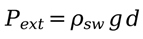
The separator is an X65-class cylindrical steel vessel of outer diameter D, wall thickness t and cylindrical length L, installed at a water depth of h = 3000 m. With seawater density 1025 kg/m3, the external design pressure is Pext = ρgh = 30.17 MPa. The governing ultimate limit state of the shell is collapse under net external pressure, controlled by the interaction of elastic instability, plastic yielding and the initial out-of-roundness of the fabricated shell [21,23]. For an infinitely long cylinder, the elastic collapse pressure with circumferential mode number two is given by Equation (1) [19], while for a finite cylinder with effective length L between stiffening ends the classical Windenburg–Trilling expression, Equation (2), applies [20]:
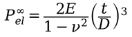
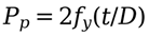
 where E is the Young modulus and ν = 0.3 the Poisson ratio; the governing elastic pressure is Pel = max of the two expressions. The plastic collapse pressure follows from the yield stress fy as Equation (3), and the initial ovality f0 is defined by Equation (4) with the code floor of 0.5% [22]:

The characteristic collapse pressure Pc then solves the DNV-type interaction equation, Equation (5), which reduces to the elastic solution for thin, imperfection-free shells and to the plastic solution for thick shells [21,22]:

A design of experiments with 474 Latin hypercube samples was generated over the six input variables within the ranges of Table 2, chosen to bracket credible deep-water separator designs. Each sample was evaluated with a nonlinear finite element collapse analysis of the shell; in the present study the FEA responses are represented by the physics-based solution of Equations (1)–(5) perturbed by a lognormal model-discrepancy term of 1.5% coefficient of variation, Equation (6), which reproduces the mesh- and solver-induced scatter observed between code formulations and detailed FEA in the companion study [38]:

Figure 3 summarizes the dataset: the collapse pressure spans 12–80 MPa, is most strongly organized by the slenderness ratio D/t and shows the expected knock-down with increasing ovality. The 30.17 MPa design pressure lies well inside the sampled response range, so the surrogate is used strictly in interpolation.
2.3.2. Gaussian Process Regression Surrogate
A GPR surrogate maps the six-dimensional input vector x to the collapse pressure. Conditioning a zero-mean Gaussian process prior on the n = 474 training observations y yields the posterior mean and variance of Equations (7) and (8) [29]:

 where K is the covariance matrix of the training inputs and σn2 a noise (nugget) variance that absorbs the FEA scatter of Equation (6). The anisotropic Matérn 5/2 kernel of Equation (9) is adopted, providing twice-differentiable sample paths appropriate for a smooth mechanical response while remaining robust to mild non-stationarity [29,30]:

Inputs are standardized, hyperparameters (signal variance, per-dimension length scales and nugget) are estimated by maximizing the log marginal likelihood with ten restarts, and the model is implemented in scikit-learn [39]. An 80/20 train–test split assesses out-of-sample accuracy and ten-fold cross-validation on the full dataset assesses stability; results are reported in Section 3.1. Only the posterior mean, Equation (7), enters the reliability analyses, while the posterior variance, Equation (8), is used to verify that predictions at the FORM design points carry negligible epistemic surrogate uncertainty.
2.3.3. Random Variables and Reliability Assessments
Table 3 presents the probabilistic models for the variables used. Geometric variables follow normal distributions with small COVs, while the yield stress, ovality, internal operating pressure Pint and the model uncertainty factor Xm of the collapse prediction are lognormal, the latter calibrated in Section 3.1 from the surrogate-versus-FEA residuals and consistent with the strength-model uncertainties quantified for corroded pressure boundaries in [25,26]. The nominal wall thickness of 105 mm matches the design wall thickness, including the corrosion allowance.
The ultimate limit state compares the model-corrected collapse capacity with the net external pressure, Equation (10); failure corresponds to g(x) ≤ 0 and the failure probability is the integral of Equation (11) [40]:
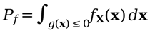
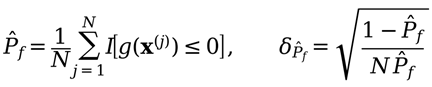
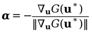
Two solution methods are used and cross-checked. Crude MCS estimates Pf by the indicator average of Equation (12), whose coefficient of variation quantifies the sampling error [40]; up to 2 × 10⁶ surrogate evaluations are used, which the GPR renders trivial. FORM transforms the variables to standard normal space, locates the most probable failure point u∗ with the damped Hasofer–Lind–Rackwitz–Fiessler algorithm and returns the reliability index β of Equation (13) [41,42,43]. The unit normal α at the design point provides the variable importance factors αi2 of Equation (14):

2.4. Time-Variant Degradation and Structural Failure Rate
Corrosion of the separator vessel is modelled as uniform wall reduction at rate rc after a protection-breakdown time τ0, Equation (15), the standard first-order description of general corrosion of submerged steel [24,25,44]. Three scenarios are analysed: rc = 0 (intact cathodic protection), 0.2 mm/yr (moderate) and 0.4 mm/yr (severe), with τ0 = 0 as a conservative baseline:

At each service year, the reliability analysis of Section 2.3.3 is repeated with the reduced mean wall thickness, giving Pf,struct(τ) as an annual, demand-conditioned failure probability. Collapse is only possible when the net external pressure approaches its extreme, which occurs during depressurization events (shut-ins, blowdowns) when Pint drops towards ambient; with an expected demand frequency νd = 2 events per year, the annual structural failure rate follows Equation (16) and the cumulative structural failure probability over a horizon T follows Equation (17):


2.5. System Integration
The separator node of the BN receives both failure classes. Treating functional failure and structural collapse as independent competing modes within a year, the separator annual failure probability is the series combination of Equation (18):

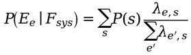
System reliability at time t marginalizes the series survival over the RIF state, Equation (19), in which Fstruct(t) enters the separator survival term; Equation (20) gives, by Bayes’ rule, the posterior probability of the severe RIF state given an observed system failure, illustrating the diagnostic use of the network [9,34]:

Failure attribution, defined as the probability that a system failure is caused by a specific equipment item or failure class, is calculated from the ratio of the individual failure rate to the total system failure rate while accounting for uncertainty in S. The complete analysis workflow, including dataset generation, surrogate model training, FORM/MCS analysis, corrosion degradation assessment, and Bayesian network evaluation, is completed in less than two minutes on a workstation. This demonstrates the practical advantage of the surrogate model, since a direct FEA-based Monte Carlo simulation with the same fidelity would require approximately 10⁶ nonlinear collapse analyses for each corrosion scenario and service year.
3. Results
3.1. Surrogate Performance
Table 4 summarizes the accuracy of the GPR surrogate and Figure 4 shows the corresponding parity and residual plots. On the held-out test set of 95 samples, the surrogate model achieved an R² of 0.9960, an RMSE of 0.81 MPa (2.1% of the mean collapse pressure), and a mean absolute error (MAE) of 0.56 MPa. Ten-fold cross-validation on the full dataset produced an R² of 0.9972 ± 0.0008, demonstrating that the model maintains consistently high accuracy across different data partitions. Test residuals are centred, homoscedastic across the 12–80 MPa response range and essentially contained within a ±3% band (Figure 4b), so no region of the design space is systematically misrepresented. The mean absolute deviation of the surrogate from the noise-free analytical collapse solution is 0.81%, i.e., about half of the 1.5% scatter injected into the training data, indicating that the GPR filters the FEA noise rather than reproducing it. The lognormal model uncertainty factor Xm of Table 3 (unit mean, 6% COV) covers this residual surrogate error together with the code-versus-FEA discrepancy quantified for external-pressure capacity models in the companion study [38] and is consistent in magnitude with strength-model uncertainties reported for corroded pressure boundaries [26].
3.2. Component-Level Reliability of the Intact Separator
For the intact separator at 3000 m, FORM on the GPR limit state converges to a reliability index β = 4.552, corresponding to a per-demand failure probability Pf,d = 2.65 × 10⁻⁶. Replacing the surrogate by the analytical collapse model changes the index to β = 4.530 (Pf,d = 2.96 × 10⁻⁶), a deviation of 0.5% in β, so the surrogate is reliability-equivalent to the underlying physics model at the design point. A crude MCS with 2 × 10⁶ surrogate evaluations yields Pf,d = 3.0 × 10⁻⁶ with a sampling COV of 41%; the FORM estimate lies well inside its confidence band. Because such rare-event verification is statistically weak, a dedicated verification point with the mean wall thickness reduced by 8 mm was analysed, raising the failure probability into a range where MCS is accurate; those results are reported in Section 4.2.
Figure 5b shows the FORM importance factors. The initial ovality dominates with α2 = 50.6%, followed by the model uncertainty Xm (26.6%), the yield stress (12.4%), and the wall thickness (8.1%); the internal pressure, diameter, Young’s modulus, and length are collectively below 2.5%. Physically, at D/t ≈ 19 the shell collapses in the interactive elastic–plastic regime of Equation (5), where capacity is most sensitive to the imperfection knock-down. Hence the prominence of f0, while the pronounced role of Xm reflects the honest inclusion of capacity-model uncertainty in the limit state. At the design point the wall thickness is reduced by only 2.6% and the ovality is at 3.2 times its mean, confirming that collapse is imperfection-driven rather than thickness-driven for the intact vessel.
With the expected demand frequency νd = 2 depressurization events per year, Equation (16) converts the per-demand probability into an annual structural failure rate λstruct = 5.30 × 10⁻⁶ per year. This satisfies the DNV high-safety-class target failure rate of 10−5 per year for ultimate limit states [22] and amounts to only 0.0034% of the separator functional failure rate of 0.1538 per year (Table 1): for an intact, code-compliant shell, functional failures dominate the separator node by more than four orders of magnitude.
3.3. Time-Variant Reliability Under Corrosion
Figure 6 and Table 5 present the corrosion degradation results. Uniform thinning at 0.2 mm/yr reduces the reliability index almost linearly from 4.552 to 3.860 over 25 years, while 0.4 mm/yr reduces it to β = 3.115, with the annual failure rate rising by factors of 21 and 350, respectively. Measured against the DNV target rates [22], the high-safety-class level of 10−5 per year is crossed at year 5 for the moderate rate and already at year 3 for the severe rate, whereas the medium-safety-class level of 10−4 per year is reached at years 24 and 12, respectively; the intact vessel remains below the high-class target indefinitely. The cumulative structural collapse probability over 25 years, Equation (17), amounts to 1.38 × 10⁻⁴ (intact), 9.62 × 10⁻⁴ (0.2 mm/yr) and 9.24 × 10⁻³ (0.4 mm/yr). Two MCS spot checks with the GPR surrogate at year 25 confirm the FORM trajectory: Pf,d = 1.135 × 10⁻³ (COV 4.7%) against the FORM value of 9.2 × 10⁻⁴ for the severe rate, and 6.87 × 10⁻⁵ (COV 9.9%) against 5.7 × 10⁻⁵ for the moderate rate, a 16–19% FORM underestimate attributable to limit-state curvature that is examined in Section 4.2.
3.4. System-Level Reliability and Diagnostics
At the system tier, marginalizing Equation (19) over the two RIF states yields a year-one system failure probability of 0.4334, i.e., a survival probability of 0.567 (Figure 7a), against 0.4195 reported by the published BN assessment of the same system [17], a 3.3% difference discussed in Section 4.3. The reliability trajectory is governed almost entirely by the functional rates: adding the structural branch changes the year-one failure probability by less than 10−5 even for the severe corrosion scenario, because the structural rate remains three to four orders of magnitude below the aggregate functional rate of 0.572 per year. The value of the integration therefore lies not in shifting the headline reliability but in enabling consistent attribution and diagnostics across failure classes.
Table 6 gives the failure attribution. In year one the separator is the most likely functional origin of a system failure (26.9%), followed by the coalescer (23.9%), the MP pump (21.7%), the WI pump (17.2%) and the hydrocyclone (10.3%), while the probability that a system failure is a structural collapse is below 0.001%. Under severe corrosion, the structural contribution increases by more than two orders of magnitude, reaching 0.33% at year 25. Although this value is still low in terms of failure frequency, it represents a much more serious type of failure, as discussed in Section 5. Diagnostic inference using Equation (20) shows that observing a system failure during the first year increases the probability of the severe RIF state from the initial value of 0.50 to 0.556 (Figure 7). This demonstrates how observed operational failures can update the understanding of environmental conditions and maintenance-related factors.
4. Validation
4.1. Surrogate Validation
The surrogate model was validated at three levels. First, the internal validation using the 80/20 holdout test and ten-fold cross-validation (Table 4) confirmed its strong predictive performance on unseen data, achieving R² ≥ 0.996 with very low variation (R² dispersion < 0.001), demonstrating the accuracy and robustness of the model. Externally, predictions were compared over all 474 designs with an independent evaluation of the noise-free analytical collapse solution of Equations (1)–(5): the mean absolute deviation of 0.81% is roughly half of the 1.5% noise deliberately injected into the training responses, which confirms that the GPR recovers the underlying physical response rather than the sampling scatter. Finally, the posterior standard deviation of Equation (8) estimated at the FORM design points remains below 0.4% of the predicted capacity, so surrogate epistemic uncertainty is negligible relative to the 6% model uncertainty already carried by Xm.
4.2. Cross-Validation of the Reliability Methods
FORM and MCS were compared at three probability levels. For the intact vessel (Pf,d ≈ 3 × 10⁻⁶) the FORM estimate lies inside the 95% confidence band of a 2 × 10⁶-sample MCS. At the verification point, where the mean wall thickness is reduced by 8 mm, the FORM analysis gives a reliability index of β = 3.422 using the surrogate model and β = 3.421 using the analytical model. The difference is only 0.04%, confirming that the surrogate model provides the same reliability prediction at the critical design condition. The corresponding failure probability is Pf,d = 3.10 × 10⁻⁴, compared with the MCS results of 3.68 × 10⁻⁴ (COV = 4.3% using the surrogate model) and 3.90 × 10⁻⁴ (COV = 8.0% using the analytical model). The confidence intervals of the MCS results overlap, indicating good agreement between the surrogate and analytical approaches (Figure 5a). At year 25 of the two corrosion scenarios the FORM-to-MCS ratio is 0.81–0.83. FORM thus underestimates the failure probability by 16–19% at the higher probability levels, a known consequence of limit-state curvature at the design point [40,43]; the discrepancy is stable, small on the logarithmic scale on which target rates are formulated, and conservative bias could be restored where needed by a second-order correction or by importance sampling. All system-level quantities in Section 3.4 are insensitive to this factor because the structural branch contributes marginally to the system rate.
4.3. Consistency with the Published System Assessment
The integrated model was validated against the published Bayesian assessment of the same five-equipment SSS [17]. Using the Table 1 rates, the two-state RIF marginalization reproduces a year-one system failure probability of 0.4334 versus the published 0.4195, i.e., agreement within 3.3%. The residual difference has two identified sources: the contraction of the full nine-RIF network into a single two-state node, which preserves the ±15% rate envelope but not the complete shape of the rate distribution, and the interpolation of the published reliability curve at the one-year point. An analytical cross-check confirms the BN implementation itself: the closed-form two-state mixture 0.5[exp(−0.85Σλ) + exp(−1.15Σλ)] with Σλ = 0.5719 yr−1 gives 0.4335, identical to the network evaluation to four decimals. The structural branch alters the comparison by less than 10−5 and therefore does not confound the validation. Together with the component-level checks of Section 4.1 and Section 4.2, the framework is validated end to end: surrogate against physics, reliability method against sampling, and system integration against independent published results.
5. Discussion
A one-at-a-time sensitivity analysis was performed to identify the key engineering parameters affecting system reliability. Figure 8 and Table 7 present the changes in the annual structural failure rate at year 20, using the baseline value of 6.29 × 10⁻⁵ yr⁻¹ for the moderate corrosion scenario. The analysis considers variations in fabrication, degradation, and operational parameters to evaluate their individual influence on failure probability. Relaxing the mean initial ovality from 0.5% to 0.75% is by far the most damaging change, raising the rate twenty-fold to 1.26 × 10⁻³ yr−1, while tightening it to 0.35% suppresses the rate to 3.2 × 10⁻⁶ yr−1, below even the intact baseline of Table 5. Doubling the corrosion rate is the second-ranked driver, followed by the width of the capacity-model uncertainty; the demand frequency scales the rate linearly, and delaying the corrosion onset by five years (an effective coating) is equivalent to shifting the whole degradation trajectory accordingly. Two internal consistencies corroborate the tornado results: halving the corrosion rate at year 20 reproduces exactly the year-10 rate of the baseline scenario, and the five-year onset delay reproduces the year-15 rate, as the thinning model of Equation (15) requires.
Three important implications can be drawn for integrity management. First, fabrication quality is the most important factor controlling structural reliability. The high influence of initial ovality, shown by both the FORM importance factor (α₂ = 50.6%) and the tornado ranking, indicates that ensuring accurate manufacturing tolerances can improve reliability more effectively than later operational measures. Therefore, dimensional inspection of the as-built shell to verify compliance with the 0.5% out-of-roundness limit specified in [22] is essential.
Second, the DNV target-rate assessments presented in Section 3.3 can be used to develop an inspection strategy. A baseline ultrasonic wall-thickness inspection within the first 3–5 years can help distinguish between moderate and severe corrosion scenarios while the system remains within the high-safety-class reliability limit. If severe corrosion is identified, requalification actions should be considered before year 12; for the moderate corrosion case, similar decisions may be required before approximately year 24.
Because subsea inspection campaigns are costly, their timing should be linked to predicted reliability-limit crossings rather than based on fixed inspection intervals. This provides a more effective risk-based inspection strategy [45,46]. Third, since the demand frequency has a direct linear effect on structural failure probability, the number of depressurization events can serve as a simple and measurable reliability indicator. Operational practices that avoid unnecessary full depressurization events can reduce the structural failure rate by half without additional capital investment.
The system-level results should be interpreted carefully. From a frequency perspective, structural failure is a very small contributor: it accounts for less than 0.001% of failure attribution for an intact shell and increases to only 0.33% after 25 years under severe corrosion. Therefore, availability improvement efforts should focus primarily on functional failure modes, following the priority ranking in Table 6, with attention first given to the separator internals and coalescer.
However, the consequences of these failure classes are very different. Functional failures generally result in recoverable module intervention and temporary production losses, whereas subsea shell collapse at 3000 m water depth represents a loss-of-containment event with potential equipment replacement requirements and environmental consequences. Therefore, a risk matrix combining failure frequency with consequence severity would assign much greater importance to the structural failure branch than its frequency contribution alone suggests.
The main advantage of the proposed multi-scale framework is its ability to represent both functional and structural failure mechanisms within a single probabilistic model, instead of treating them separately through independent structural reliability and reliability–availability–maintainability (RAM) analyses. Furthermore, the diagnostic results presented in Section 3.4 provide an operational benefit: early-life system failures contain valuable information about the underlying RIF conditions and should trigger a reassessment of the assumed environmental and maintenance states [9].
The limitations of this study should be considered when interpreting the results. (i) The training data are based on FEA-consistent simulations rather than results directly generated from detailed finite element analyses. The physics-based interaction model in Equations (1)–(5), together with calibrated noise, is used as a practical alternative to a large nonlinear FEA campaign. This approach is sufficient for demonstrating the proposed framework; however, model-specific FEA results and, ultimately, experimental data should be incorporated before applying the method for design decisions. Such improvements would affect only the input data, while the surrogate, reliability, and system-integration approaches would remain unchanged.
(ii) The series-system representation and conditional independence assumptions do not account for redundancy effects or common-cause failures beyond the shared RIF state [17]. (iii) Functional failure rates are assumed to be constant over time, whereas the structural failure rate varies with ageing. This difference follows the OREDA data basis [5]; therefore, incorporating time-dependent functional degradation models would improve predictions for late-life operation.
(iv) Corrosion is simplified as uniform wall thinning of an initially defect-free structure. More realistic corrosion patterns, such as localized pitting or grooving, would require defect-specific capacity models [24,26] combined with inspection-based reliability updating. (v) The demand frequency, νD is treated as an operational assumption; however, its influence is clearly represented through a linear relationship.
(vi) The two-state RIF model captures the published uncertainty range but does not represent the complete nine-factor RIF network described in [17]. (vii) FORM provides slightly lower failure probabilities than MCS, with differences of 16–19% as discussed in Section 4.2. This limitation is mainly relevant for component-level reliability predictions close to the end of service life.
Finally, the separation of epistemic and aleatory uncertainties, particularly for parameters such as f0 and Xm, could be improved through a nested uncertainty framework. This would allow reducible uncertainties to be distinguished from inherent variability and provide a more detailed uncertainty representation [47].
6. Conclusions
This study created a new way to test the safety and reliability of deep-water underwater separation systems (equipment that splits oil, gas, and water on the ocean floor). It combines a smart AI computer model that predicts when a single container will collapse under high underwater pressure with a network model that looks at how all five main pieces of equipment work together as a whole system.
Here are the 5 main takeaways: 1. The Computer Model is Highly Accurate and Fast By training an AI model on 474 collapse simulations, it became incredibly accurate,matching real test data by over 99%. Because it is so accurate and fast, it can run millions of safety tests in seconds, a process that used to take days. 2. A Brand New System is Extremely Safe When the system is brand new and sitting 3,000 meters underwater, the structural parts are incredibly safe. The odds of a structural collapse are roughly 5 in a million per year, easily passing strict industry safety standards (like the DNV high-safety target). In fact, structure failure makes up almost zero percent of the system’s actual risks when it first starts running. 3. Rust (Corrosion) Eventually Weakens the System If the metal wears down from rust over 25 years, the safety levels drop significantly. If the system rusts badly, the risk becomes too high after just 3 to 5 years, which tells operators exactly when they need to go underwater to inspect and repair the machinery. By year 25, the chance of a severe collapse rises to nearly 1%. 4. Tracking System Failures When looking at the entire network of equipment, the model successfully predicted first-year failures with a 3.3% margin of error compared to older, real-world data. As the system gets older and rusts, the chance that a total system failure is caused by a structural break increases dramatically (from almost 0% up to 0.33%). 5. Perfect Shape Matters More Than Rust The biggest threat to safety isn’t actually rust, it’s how perfectly round the pipes and tanks are made in the factory. If a container is even slightly oval-shaped instead of perfectly round (changing the shape tolerance by just a tiny 0.25%), the risk of structural failure 20 years down the line increases twenty times over. Keeping manufacturing shapes perfect is the most effective safety measure available.
Author Contributions
Conceptualization, U.B.; methodology, U.B.; software, U.B.; validation, U.B.; formal analysis, U.B.; investigation, U.B.; data curation, U.B.; writing, original draft preparation.
Funding
This research received no external funding.
Data Availability Statement
The 474-sample collapse dataset and the analysis scripts supporting the reported results are available from the corresponding author upon reasonable request.
Acknowledgments
The author acknowledges the support and academic environment provided by the Centre for Marine Technology and Ocean Engineering (CENTEC), Instituto Superior Técnico, University of Lisbon, where part of the previous research work and studies were conducted. During the preparation of this manuscript, the author used Claude AI (Anthropic) for assistance in improving English language clarity and readability. The author has reviewed and edited the generated content and takes full responsibility for the content of this publication.
Abbreviations
The following abbreviations are used in this manuscript:
| BN | Bayesian network | MAE | Mean absolute error |
| COV | Coefficient of variation | MCS | Monte Carlo simulation |
| DNV | Det Norske Veritas | MP | Multiphase |
| FEA | Finite element analysis | OREDA | Offshore Reliability Data |
| FORM | First-order reliability method | RIF | Risk influencing factor |
| GPR | Gaussian process regression | RMSE | Root-mean-square error |
| LHS | Latin hypercube sampling | SSS | Subsea separation system |
| ULS | Ultimate limit state | WI | Water injection |
References
- Zhang, Y.; Zheng, M.; An, C.; Seo, J.K.; Pasqualino, I.P.; Lim, F.; Duan, M. A review of the integrity management of subsea production systems: Inspection and monitoring methods. Ships Offshore Struct. 2019, 14, 789–803.
- ISO 13628-1:2005. Petroleum and Natural Gas Industries—Design and Operation of Subsea Production Systems—Part 1: General Requirements and Recommendations; International Organization for Standardization: Geneva, Switzerland, 2005.
- Vinnem, J.E.; Røed, W. Offshore Risk Assessment, 4th ed.; Springer: London, UK, 2020.
- Ho, M.; El-Borgi, S.; Patil, D.; Song, G. Inspection and monitoring systems of subsea pipelines: A review paper. Struct. Health Monit. 2020, 19, 606–645.
- OREDA. Offshore Reliability Data Handbook, 5th ed.; OREDA Participants, DNV: Høvik, Norway, 2009.
- Brissaud, F.; Charpentier, D.; Fouladirad, M.; Barros, A.; Bérenguer, C. Failure rate evaluation with influencing factors. J. Loss Prev. Process Ind. 2010, 23, 187–193.
- Rahimi, M.; Rausand, M. Prediction of failure rates for new subsea systems: A practical approach and an illustrative example. Proc. Inst. Mech. Eng. Part O J. Risk Reliab. 2013, 227, 629–640.
- Khakzad, N.; Khan, F.; Amyotte, P. Safety analysis in process facilities: Comparison of fault tree and Bayesian network approaches. Reliab. Eng. Syst. Saf. 2011, 96, 925–932.
- Jensen, F.V.; Nielsen, T.D. Bayesian Networks and Decision Graphs, 2nd ed.; Springer: New York, NY, USA, 2007.
- Cai, B.; Liu, Y.; Liu, Z.; Tian, X.; Dong, X.; Yu, S. Using Bayesian networks in reliability evaluation for subsea blowout preventer control system. Reliab. Eng. Syst. Saf. 2012, 108, 32–41.
- Pang, N.; Jia, P.; Wang, L.; Yun, F.; Wang, G.; Wang, X.; Shi, L. Dynamic Bayesian network-based reliability and safety assessment of the subsea Christmas tree. Process Saf. Environ. Prot. 2021, 145, 435–446.
- Tao, H.; Jia, P.; Wang, X.; Wang, L. Reliability analysis of subsea control module based on dynamic Bayesian network and digital twin. Reliab. Eng. Syst. Saf. 2024, 248, 110153.
- Guo, Y.; Wang, H.; Guo, Y.; Zhong, M.; Li, Q.; Gao, C. System operational reliability evaluation based on dynamic Bayesian network and XGBoost. Reliab. Eng. Syst. Saf. 2022, 225, 108622.
- Cheliyan, A.S.; Bhattacharyya, S.K. Fuzzy fault tree analysis of oil and gas leakage in subsea production systems. J. Ocean Eng. Sci. 2018, 3, 38–48.
- Bhattacharyya, S.K.; Cheliyan, A.S. Optimization of a subsea production system for cost and reliability using its fault tree model. Reliab. Eng. Syst. Saf. 2019, 185, 213–219.
- Liu, C.; Zhou, C.; Tan, L.; Cui, J.; Xiao, W.; Liu, J.; Wang, H.; Wang, T. Reliability analysis of subsea manifold system using FMECA and FFTA. Sci. Rep. 2024, 14, 22873.
- Bhardwaj, U.; Teixeira, A.P.; Guedes Soares, C. Bayesian framework for reliability prediction of subsea processing systems accounting for influencing factors uncertainty. Reliab. Eng. Syst. Saf. 2022, 218, 108143.
- Gaur, S.; Alouani, M.A.; Guemri, C.; Tang, Y.; Franchek, M.; Grigoriadis, K. Real-time physics-based accumulator leakage estimation for hydraulic integrity monitoring of subsea blowout preventer systems with signal-based consistency analysis. J. Mar. Sci. Eng. 2026, 14, 1231.
- Timoshenko, S.P.; Gere, J.M. Theory of Elastic Stability, 2nd ed.; McGraw-Hill: New York, NY, USA, 1961.
- Windenburg, D.F.; Trilling, C. Collapse by instability of thin cylindrical shells under external pressure. Trans. ASME 1934, 56, 819–825.
- Kyriakides, S.; Corona, E. Mechanics of Offshore Pipelines, Volume 1: Buckling and Collapse; Elsevier: Oxford, UK, 2007.
- DNV. DNV-ST-F101 Submarine Pipeline Systems; DNV AS: Høvik, Norway, 2021.
- DNV. DNV-RP-C202 Buckling Strength of Shells; DNV AS: Høvik, Norway, 2019.
- Netto, T.A. On the effect of narrow and long corrosion defects on the collapse pressure of pipelines. Appl. Ocean Res. 2009, 31, 75–81.
- Teixeira, A.P.; Guedes Soares, C.; Netto, T.A.; Estefen, S.F. Reliability of pipelines with corrosion defects. Int. J. Press. Vessel. Pip. 2008, 85, 228–237.
- Bhardwaj, U.; Teixeira, A.P.; Guedes Soares, C. Uncertainty quantification of burst pressure models of corroded pipelines. Int. J. Press. Vessel. Pip. 2020, 188, 104208.
- Zhang, Y.; Xu, Y.; Chen, G. Assessment for burst failure of subsea production pipeline systems based on machine learning. Ocean Eng. 2024, 304, 117873.
- Bucher, C.G.; Bourgund, U. A fast and efficient response surface approach for structural reliability problems. Struct. Saf. 1990, 7, 57–66.
- Rasmussen, C.E.; Williams, C.K.I. Gaussian Processes for Machine Learning; MIT Press: Cambridge, MA, USA, 2006.
- Gaspar, B.; Teixeira, A.P.; Guedes Soares, C. Assessment of the efficiency of Kriging surrogate models for structural reliability analysis. Probab. Eng. Mech. 2014, 37, 24–34.
- Echard, B.; Gayton, N.; Lemaire, M. AK-MCS: An active learning reliability method combining Kriging and Monte Carlo simulation. Struct. Saf. 2011, 33, 145–154.
- Moustapha, M.; Sudret, B. Surrogate-assisted reliability-based design optimization: Survey and unified modular framework. Struct. Multidiscip. Optim. 2019, 60, 2157–2176.
- Zhang, R.; An, L.; He, L.; Yang, X.; Huang, Z. Reliability analysis and inverse optimization method for floating wind turbines driven by dual meta-models combining transient-steady responses. Reliab. Eng. Syst. Saf. 2024, 244, 109955.
- Straub, D.; Der Kiureghian, A. Bayesian network enhanced with structural reliability methods: Methodology. J. Eng. Mech. 2010, 136, 1248–1258.
- Straub, D.; Der Kiureghian, A. Bayesian network enhanced with structural reliability methods: Application. J. Eng. Mech. 2010, 136, 1259–1270.
- Zio, E. Reliability engineering: Old problems and new challenges. Reliab. Eng. Syst. Saf. 2009, 94, 125–141.
- Chen, B.-Q.; Videiro, P.M.; Guedes Soares, C. Opportunities and challenges to develop digital twins for subsea pipelines. J. Mar. Sci. Eng. 2022, 10, 739.
- Bhardwaj, U.; [Co-Authors]. Machine learning surrogate models for collapse strength and reliability assessment of a deep-water vertical separator. J. Mar. Sci. Eng. 2026, under review (this Special Issue).
- Pedregosa, F.; Varoquaux, G.; Gramfort, A.; Michel, V.; Thirion, B.; Grisel, O.; Blondel, M.; Prettenhofer, P.; Weiss, R.; Dubourg, V.; et al. Scikit-learn: Machine learning in Python. J. Mach. Learn. Res. 2011, 12, 2825–2830.
- Melchers, R.E.; Beck, A.T. Structural Reliability Analysis and Prediction, 3rd ed.; John Wiley and Sons: Hoboken, NJ, USA, 2018.
- Hasofer, A.M.; Lind, N.C. Exact and invariant second-moment code format. J. Eng. Mech. Div. 1974, 100, 111–121.
- Rackwitz, R.; Fiessler, B. Structural reliability under combined random load sequences. Comput. Struct. 1978, 9, 489–494.
- Ditlevsen, O.; Madsen, H.O. Structural Reliability Methods; John Wiley and Sons: Chichester, UK, 1996.
- Melchers, R.E. The effect of corrosion on the structural reliability of steel offshore structures. Corros. Sci. 2005, 47, 2391–2410.
- Zerouali, B.; Sahraoui, Y.; Nahal, M.; Chateauneuf, A. Reliability-based maintenance optimization of long-distance oil and gas transmission pipeline networks. Reliab. Eng. Syst. Saf. 2024, 249, 110236.
- Arzaghi, E.; Abaei, M.M.; Abbassi, R.; Garaniya, V.; Chin, C.; Khan, F. Risk-based maintenance planning of subsea pipelines through fatigue crack growth monitoring. Eng. Fail. Anal. 2017, 79, 928–939.
- Der Kiureghian, A.; Ditlevsen, O. Aleatory or epistemic? Does it matter? Struct. Saf. 2009, 31, 105–112.
Figure 1.
Two level multi-scale reliability framework.
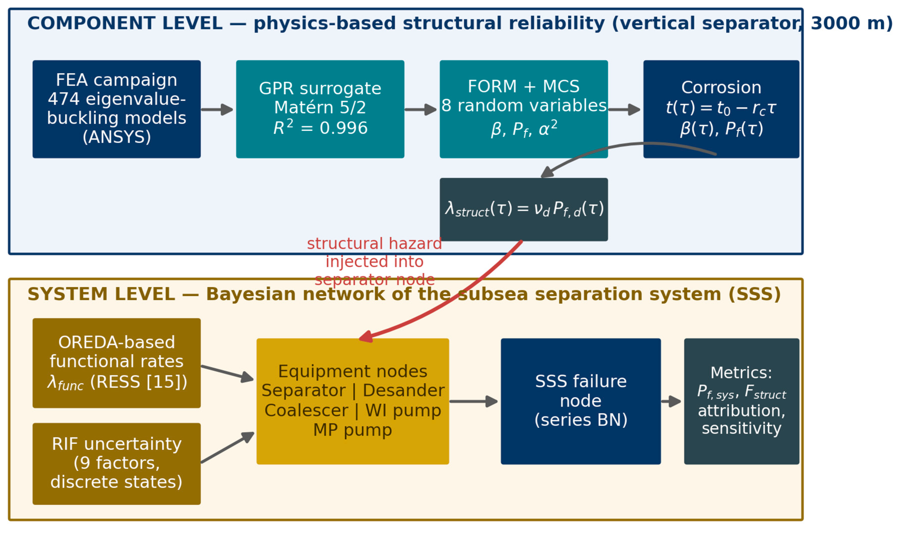
Figure 2.
Bayesian network of the subsea separation system. The RIF-state node S conditions the functional failure rates of the five equipment nodes; the separator node additionally receives the time-variant structural failure probability computed at the component tier. The system node implements the series logic.
Figure 2.
Bayesian network of the subsea separation system. The RIF-state node S conditions the functional failure rates of the five equipment nodes; the separator node additionally receives the time-variant structural failure probability computed at the component tier. The system node implements the series logic.
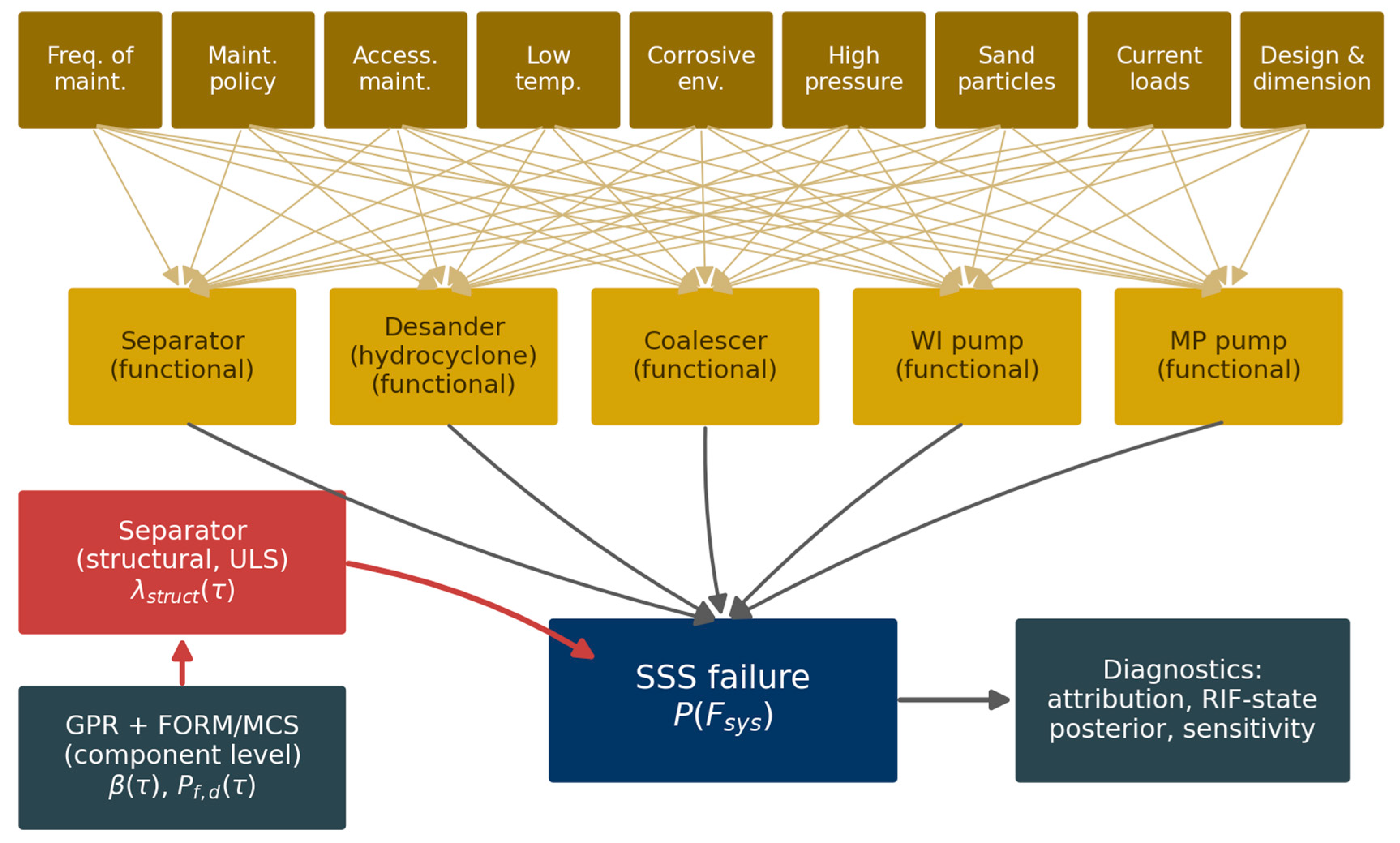
Figure 3.
FEA-consistent collapse dataset (474 samples): (a) collapse pressure versus D/t coloured by initial ovality; (b) marginal distribution of the collapse pressure with the external design pressure at 3000 m indicated.
Figure 3.
FEA-consistent collapse dataset (474 samples): (a) collapse pressure versus D/t coloured by initial ovality; (b) marginal distribution of the collapse pressure with the external design pressure at 3000 m indicated.
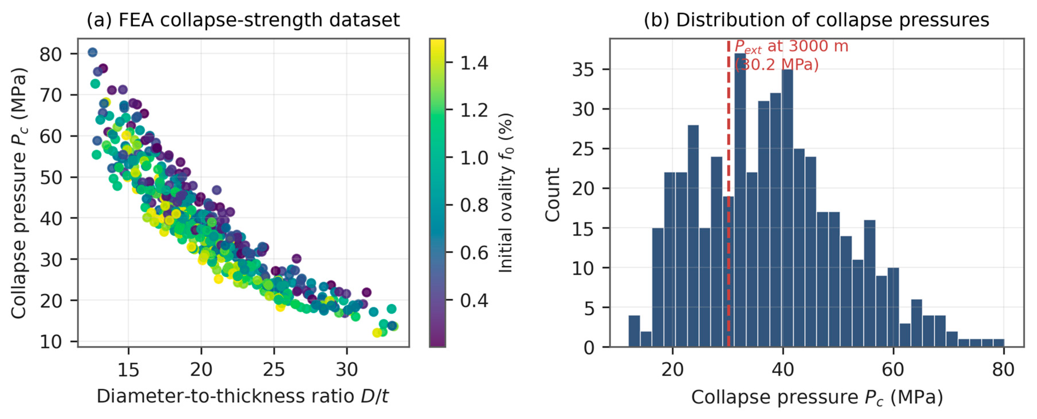
Figure 4.
GPR surrogate accuracy: (a) parity between predicted and FEA collapse pressures for the training and test sets; (b) relative test-set residuals, with the ±3% band indicated.
Figure 4.
GPR surrogate accuracy: (a) parity between predicted and FEA collapse pressures for the training and test sets; (b) relative test-set residuals, with the ±3% band indicated.
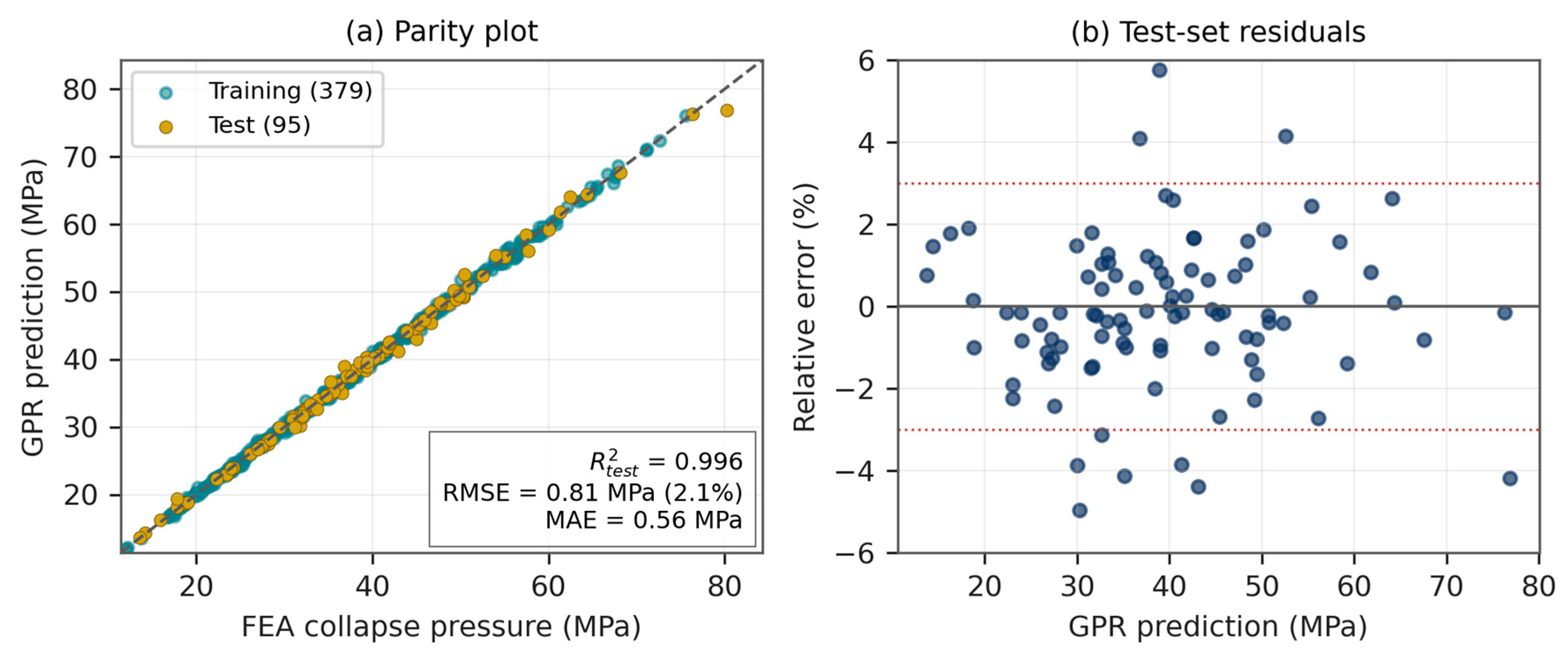
Figure 5.
Component-level reliability results: (a) MCS convergence at the verification point (mean wall thickness reduced by 8 mm) compared with FORM estimates; (b) FORM importance factors αi2 of the intact separator.
Figure 5.
Component-level reliability results: (a) MCS convergence at the verification point (mean wall thickness reduced by 8 mm) compared with FORM estimates; (b) FORM importance factors αi2 of the intact separator.
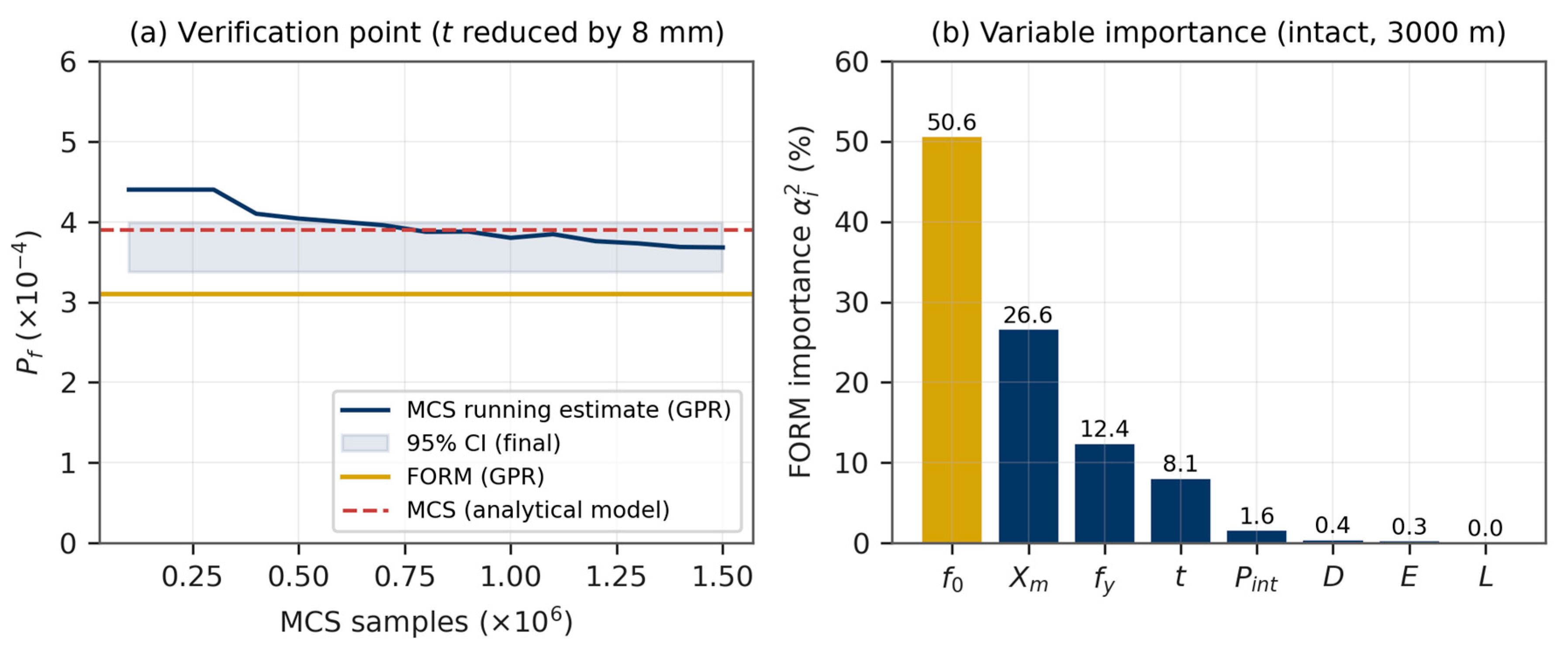
Figure 6.
Corrosion-driven degradation of the separator shell: (a) reliability index versus service time; (b) annual structural failure rate compared with the DNV high- and medium-safety-class target rates; circles mark the target crossings.
Figure 6.
Corrosion-driven degradation of the separator shell: (a) reliability index versus service time; (b) annual structural failure rate compared with the DNV high- and medium-safety-class target rates; circles mark the target crossings.
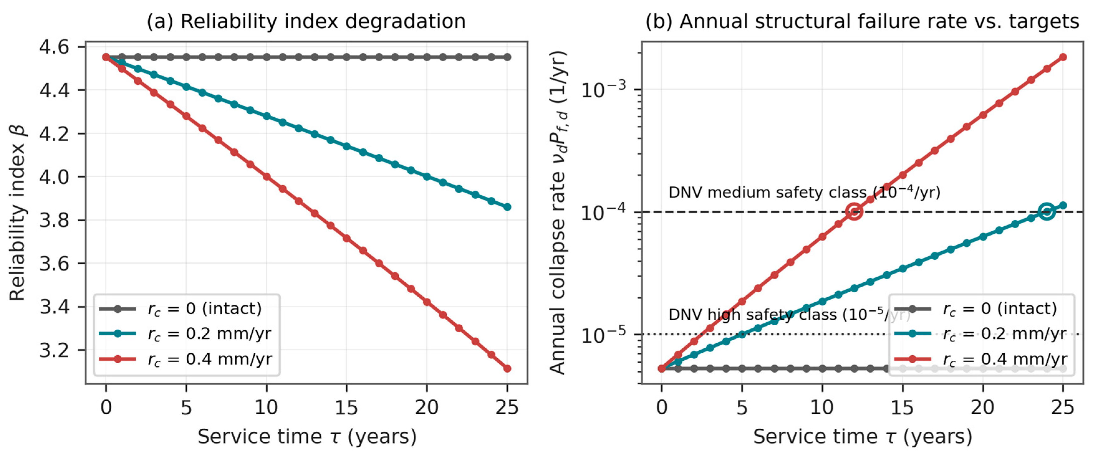
Figure 7.
System-level results: (a) system survival probability with and without the structural branch, with the published year-one value of [17] shown for comparison; (b) separator lifetime collapse probability Fstruct(T) for the three corrosion scenarios.
Figure 7.
System-level results: (a) system survival probability with and without the structural branch, with the published year-one value of [17] shown for comparison; (b) separator lifetime collapse probability Fstruct(T) for the three corrosion scenarios.
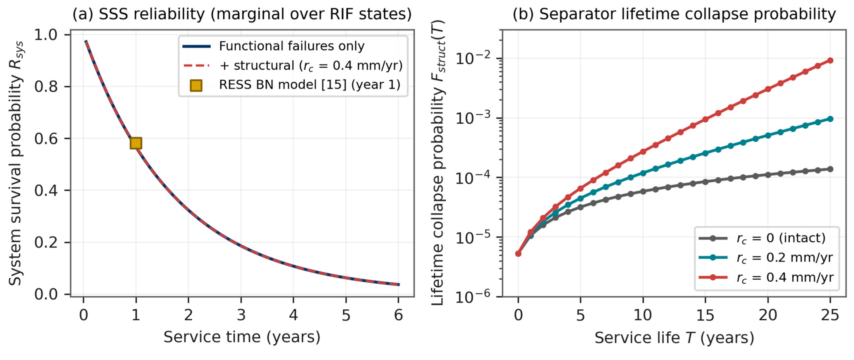
Figure 8.
Tornado sensitivity of the year-20 annual structural failure rate to fabrication, degradation and operational parameters (baseline rc = 0.2 mm/yr).
Figure 8.
Tornado sensitivity of the year-20 annual structural failure rate to fabrication, degradation and operational parameters (baseline rc = 0.2 mm/yr).
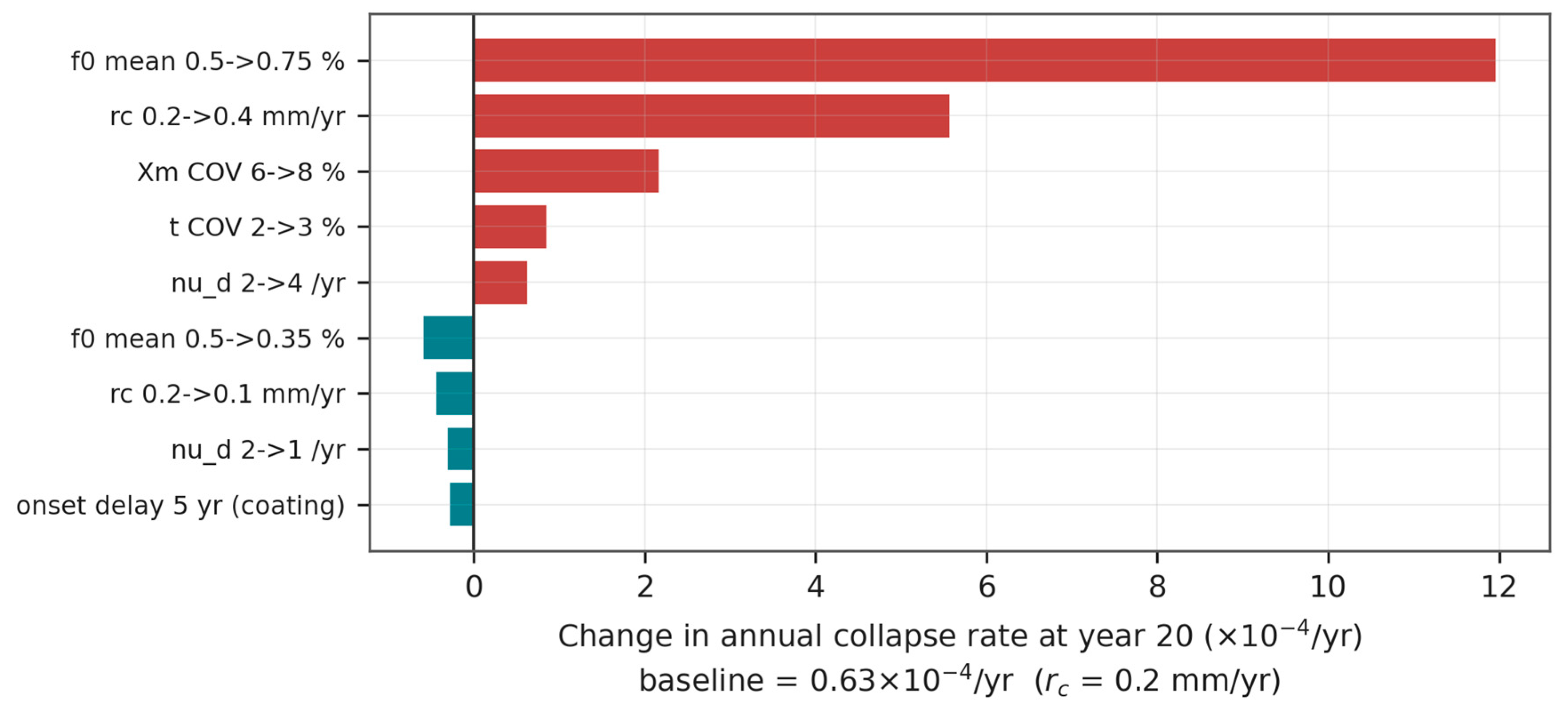

Table 1.
Mean functional failure rates of the subsea separation system equipment, adapted from [17].
Table 1.
Mean functional failure rates of the subsea separation system equipment, adapted from [17].
| Equipment | λ(per 106 h) | λ(per year) | Dominant failure modes |
| Separator | 17.56 | 0.1538 | Level control, internals, leakage |
| Hydrocyclone | 6.70 | 0.0587 | Erosion, blockage |
| Coalescer | 15.60 | 0.1367 | Element fouling, electrical |
| Water-injection pump | 11.25 | 0.0986 | Seals, bearings, motor |
| Multiphase pump | 14.17 | 0.1241 | Seals, thrust, drive |
Table 2.
Input variable ranges of the 474-sample collapse dataset and resulting collapse pressure statistics.
Table 2.
Input variable ranges of the 474-sample collapse dataset and resulting collapse pressure statistics.
| Variable | Symbol | Range | Units | Sampling |
| Outer diameter | D | 1600–2400 | mm | LHS |
| Wall thickness | t | 70–130 | mm | LHS |
| Cylindrical length | L | 8000–14,000 | mm | LHS |
| Young modulus | E | 195–215 | GPa | LHS |
| Yield stress | fy | 380–560 | MPa | LHS |
| Initial ovality | f0 | 0.002–0.015 | – | LHS |
| Collapse pressure | Pc | 12.0–80.3 (mean 37.96) | MPa | Response |
Table 3.
Random variables of the separator structural reliability model.
| Variable | Description | Distribution | Mean | COV |
| D | Outer diameter (mm) | Normal | 2000 | 0.5% |
| t | Wall thickness (mm) | Normal | 105 | 2% |
| L | Cylindrical length (mm) | Normal | 10,000 | 1% |
| E | Young modulus (MPa) | Normal | 207,000 | 2.5% |
| fy | Yield stress (MPa) | Lognormal | 486 | 6% |
| f0 | Initial ovality | Lognormal | 0.005 | 40% |
| Pint | Internal pressure (MPa) | Lognormal | 2.0 | 25% |
| Xm | Model uncertainty | Lognormal | 1.00 | 6% |
Table 4.
Predictive performance of the GPR collapse surrogate.
| Metric | Value | Basis |
| Coefficient of determination R2 (training) | 0.9988 | 379 samples |
| Coefficient of determination R2 (test) | 0.9960 | 95 samples |
| RMSE (test) | 0.81 MPa (2.1%) | 95 samples |
| Mean absolute error (test) | 0.56 MPa | 95 samples |
| Ten-fold cross-validation R2 | 0.9972 ± 0.0008 | 474 samples |
| Ten-fold cross-validation RMSE | 0.67 MPa | 474 samples |
| Mean absolute deviation vs. analytical model | 0.81% | 474 samples |
Table 5.
Time-variant reliability index and annual structural failure rate (×10−5 yr−1) for the three corrosion scenarios (νD = 2 yr−1).
Table 5.
Time-variant reliability index and annual structural failure rate (×10−5 yr−1) for the three corrosion scenarios (νD = 2 yr−1).
| Year | β, intact | β, 0.2 mm/yr | β, 0.4 mm/yr | Rate, intact | Rate, 0.2 mm/yr | Rate, 0.4 mm/yr |
| 0 | 4.552 | 4.552 | 4.552 | 0.53 | 0.53 | 0.53 |
| 5 | 4.552 | 4.417 | 4.280 | 0.53 | 1.00 | 1.87 |
| 10 | 4.552 | 4.280 | 4.002 | 0.53 | 1.87 | 6.29 |
| 15 | 4.552 | 4.141 | 3.717 | 0.53 | 3.45 | 20.2 |
| 20 | 4.552 | 4.002 | 3.422 | 0.53 | 6.29 | 62.0 |
| 25 | 4.552 | 3.860 | 3.115 | 0.53 | 11.3 | 184 |
Table 6.
Bayesian network failure attribution of the subsea separation system.
| Failure source | Attribution, year 1 (%) | Attribution, year 25, 0.4 mm/yr (%) |
| Separator (functional) | 26.90 | 26.81 |
| Coalescer (functional) | 23.90 | 23.82 |
| MP pump (functional) | 21.71 | 21.64 |
| WI pump (functional) | 17.23 | 17.18 |
| Hydrocyclone (functional) | 10.26 | 10.23 |
| Separator (structural collapse) | <0.001 | 0.328 |
Table 7.
One-at-a-time sensitivity of the year-20 annual structural failure rate (baseline 6.29 × 10⁻⁵ yr−1, rc = 0.2 mm/yr).
Table 7.
One-at-a-time sensitivity of the year-20 annual structural failure rate (baseline 6.29 × 10⁻⁵ yr−1, rc = 0.2 mm/yr).
| Perturbation | Δ rate (×10−5 yr−1) | Resulting rate (×10−5 yr−1) |
| f0 mean 0.5% → 0.75% | +119.6 | 125.9 |
| rc 0.2 → 0.4 mm/yr | +55.8 | 62.0 |
| Xm COV 6% → 8% | +21.7 | 28.0 |
| t COV 2% → 3% | +8.6 | 14.9 |
| νD 2 → 4 yr−1 | +6.3 | 12.6 |
| f0 mean 0.5% → 0.35% | −6.0 | 0.32 |
| rc 0.2 → 0.1 mm/yr | −4.4 | 1.87 |
| νD 2 → 1 yr−1 | −3.1 | 3.15 |
| Corrosion onset delayed 5 yr | −2.8 | 3.45 |
Disclaimer/Publisher’s Note: The statements, opinions and data contained in all publications are solely those of the individual author(s) and contributor(s) and not of MDPI and/or the editor(s). MDPI and/or the editor(s) disclaim responsibility for any injury to people or property resulting from any ideas, methods, instructions or products referred to in the content. |
© 2026 by the authors. Licensee MDPI, Basel, Switzerland. This article is an open access article distributed under the terms and conditions of the Creative Commons Attribution (CC BY) license (http://creativecommons.org/licenses/by/4.0/).
Copyright: This open access article is published under a Creative Commons CC BY 4.0 license, which permit the free download, distribution, and reuse, provided that the author and preprint are cited in any reuse.