

Submitted:
23 July 2026
Posted:
24 July 2026
You are already at the latest version
Abstract
Quantitative morphology can extend taxonomic comparison across preserved specimens, living individuals, and calibrated images, but an incomplete reference library may cause confident assignment of an unrepresented species to a known class. We stress-tested a flexible classifier-modelling system using 70 Taiwanese Euterpnosia specimens, five reference classes, and 20 external characters measurable without wing spreading. Twenty repeats of five-fold nested cross-validation yielded 95.93% accuracy and 94.71% balanced accuracy for a feature-screened multinomial model. An all-character multinomial model was modestly more accurate (96.57%; paired difference 0.64 percentage points). Abstention increased reliability, although no agreement rule consistently surpassed simpler confidence rejection. With known and omitted specimens given equal biological weight, leave-one-species-out experiments rejected E. chilanensis, E. olivacea, and E. hoppo in 100%, 100%, and 92.0% of specimen-repeat decisions, whereas omitted E. alpina and E. varicolor were rejected only 21.1% and 35.0% of the time. Reference absence was therefore detectable only when an omitted taxon occupied distinguishable measured morphospace. A provisional quantitative screening tree translated multivariate structure into auditable thresholds. Integrating flexible character acquisition, leakage-resistant comparison, explicit abstention, reference-gap diagnosis, and interpretable screening provides an original workflow for classifier-assisted taxonomy. The protocol is technically applicable to females, but female-specific performance remains untested.
Keywords:
Cicadidae
; classifier modelling
; integrative morphometrics
; incomplete reference library
; open-set recognition
; reject option
; species identification
1. Introduction
Taxonomy provides the names, diagnoses, and testable organismal units on which biodiversity science depends, yet the demand for reliable identifications exceeds specialist capacity. The taxonomic impediment reflects declining expertise, insufficient support for revisions, inaccessible collections, and the time required to characterize variation across specimen series [1,2,3]. A fauna-wide assessment documented a severe decline in identification expertise across many animal groups [4], while a global analysis of more than 150 million collection records showed that declining specimen acquisition is eroding the temporal, geographic, and taxonomic coverage of natural-history infrastructure [5]. Misidentification in collections can propagate into biodiversity research [6], and recent computer-vision auditing demonstrates that mislabeled museum specimens can be detected at useful scale but still require expert or genetic verification [7]. Computational systems should therefore extend the reach, consistency, and auditability of expert taxonomy without confusing prediction with nomenclatural authority.
Modern taxonomy comprises distinct but connected tasks—discovery, delimitation, diagnosis, description, and specimen determination—and no classifier can substitute for all five [13]. The identification problem is especially acute in groups whose species differ weakly in external morphology. Conventional keys commonly reduce complex continuous variation to a small number of verbal character states. Such keys are indispensable, but their performance may decline when diagnostic states overlap, when the available series underrepresents intraspecific variation, when an early couplet is misread, or when identification depends on dissection. Molecular evidence can reveal cryptic diversity and test evolutionary hypotheses, but it does not remove methodological judgment: marker conflict, sampling bias, model choice, and dependence on well-curated trait references can complicate diagnosis and delimitation [9]. Destructive sampling, DNA degradation in historical material, contamination, cost, and curatorial restrictions can further limit molecular work on rare or name-bearing specimens. Non-destructive DNA protocols have improved substantially [10,11,12], but they remain complementary to non-destructive phenotypic evidence rather than eliminating the need for it.
Quantitative external morphology offers a complementary route. A classifier need not be tied to a single acquisition medium: homologous characters may be measured directly from preserved specimens or living individuals, extracted from calibrated contemporary or historical images, or assembled by combining compatible sources. Once units, definitions, and anatomical homology are harmonized, these measurements can be expressed in a common character space. This flexibility does not make a photograph—or any single character source—sufficient for naming a species, but it enables explicit comparison before dissection or additional collecting. Recent entomological literature documents the rapid expansion of geometric morphometrics from taxonomic applications toward multimodal and machine-learning workflows [13]. Morphometric and machine-learning studies have distinguished insects from wing outlines or landmarks [14,15,16,17], while a recent Insects study combined routine wing and abdominal measurements with an interpretable XGBoost classifier for honey-bee subspecies [18]. Image-centred systems now range from large arthropod training libraries and fine-grained insect classifiers to live-insect detection and visual–acoustic multimodal recognition [19,20,21,22]. Most such studies emphasize closed-set accuracy. In taxonomic practice, however, the consequential error is often not confusion among represented species but confident assignment of a specimen whose species is absent from the library.
Classification with a reject option formalizes the choice to abstain when evidence is insufficient [23,24,25]. Open-set recognition addresses the related but distinct problem of classes absent during training [26,27]. These principles are highly relevant to taxonomy because reference libraries are rarely complete. Our classifier-modelling system does not claim invention of multinomial regression, regularized discriminant analysis [28], Mahalanobis distance, or classification trees. Its original contribution is their taxonomically structured integration with flexible morphological measurement, nested validation, explicit abstention, empirical leave-one-species-out stress tests, and a measured screening tree. Earlier applications by the authors developed elements of the broader programme through new-species research, numerical taxonomy, integrative morphometrics, numerical ecology, and physiological–climate classification [29,30,31,32,33,34,35]; the present study is the first to expose the complete decision architecture and test where it fails under an incomplete species library.
The cicada genus Euterpnosia provides a demanding test. Traditional cicada classification is male centred because calling songs and male genitalia supply important evidence, whereas females lack calling songs and may be difficult to identify morphologically. External quantitative characters are not intrinsically restricted to one sex and can be measured from females, living individuals, and intact specimens, although sex-specific accuracy must be tested with adequate female samples. Taiwanese Euterpnosia species may differ in song while remaining similar in preserved external morphology, and dissection is undesirable for types and valuable historical material. Earlier quantitative work within the same research programme contributed to the hypothesis later formalized in the conventional description of E. chilanensis [36]. That history motivates the workflow but is not treated as independent prospective validation.
Earlier classifier-modelling applications emphasized fit to reference data. Contemporary predictive standards require separation of fitting, model selection, and evaluation: feature selection before cross-validation produces optimistic error estimates [37], small data sets require leakage-resistant resampling [38], and probability scores require calibration assessment using proper scoring rules and reliability diagnostics [39,40]. Most importantly, a model trained on five named classes should not be forced to assign every specimen to one of them.
We tested three general hypotheses: (1) quantitative external morphological characters contain enough information to classify unseen measurements drawn from the same incompletely annotated reference domain; (2) abstention trades coverage for reliability, but a compound agreement rule need not outperform simpler confidence rejection; and (3) an omitted species is rejected only when it is sufficiently separated from represented classes in measured morphospace. We further compared eight classifiers on identical folds, quantified calibration uncertainty at the specimen level, converted multivariate structure into a provisional screening tree, and defined where model output must stop short of species delimitation and nomenclature.
2. Materials and Methods
Specimens and analytical roles
Specimens and image records originated from field surveys and the National Museum of Natural Science, Taichung (NMNS); Taiwan Forestry Research Institute, Taipei (TFRI); Department of Entomology, National Taiwan University, Taipei (NTU); and the Laboratory of Systematic Entomology, Hokkaido University, Sapporo (SEHU). Living individuals were captured briefly, observed, positioned without injury, photographed with a scale for documentary measurement, and immediately released at the capture locality. They were not killed, dissected, chemically treated, or subjected to an experimental intervention, and no injury or observable adverse effect resulted from the brief handling. Field localities were outside national parks, nature reserves, protected areas, and other zones subject to collection restrictions. Pinned and type material was photographed without destructive preparation whenever possible. The holotype and all paratypes of E. chilanensis are deposited in NMNS; the original description did not publish individual accession numbers [36].
Data roles were assigned before model evaluation. Seventy specimens with complete measurements for 71 characters formed the model-development set. These specimens represented five operational reference classes: E. chilanensis (class 1), E. alpina (class 2), E. varicolor including the holotype of E. elongata (class 3), E. olivacea including specimens historically identified as E. kotoshoensis (class 4), and E. hoppo (class 5). The holotype of E. elongata and historically identified E. kotoshoensis material contributed to reference-class definition and are not independent validation. Class labels were taxonomic hypotheses supplied to prediction, not conclusions produced by it. The series was predominantly male because traditional cicada collections and diagnoses emphasize male calling songs and genitalia. The measurement protocol itself uses external homologous characters and is technically applicable to females, as illustrated by measurement and description of female E. chilanensis material [36]; however, the reconciled file lacks a complete specimen-level sex field, so female classification performance cannot be estimated. Locality, collection year, imaging session, preservation condition, and accession metadata are likewise incomplete. We therefore evaluate unseen measurements drawn from the same incompletely annotated reference domain, not transfer to new populations, sexes, operators, or imaging domains.
The source workbook contained 132 specimen columns. Six records with explicitly uncertain varicolor labels and one record labelled `un-1` were excluded before analysis. After removal of records duplicated in the model-development set, 55 specimens remained in the taxonomic-projection set. These records were selected for their relevance to nomenclature, type-locality interpretation, species revision, or assessment of taxa absent from model development. Projection specimens were never used to rank characters, tune regularization, estimate accuracy, or calibrate rejection.
Morphological character acquisition
Dorsal images were obtained using a Canon 6D camera with a Canon EF 100 mm f/2.8L Macro IS USM lens mounted on a copy stand. A scale included in each measurement image was used to calibrate coordinates in tpsDig2. The broader source material also included external morphological information obtained from preserved specimens and living individuals rather than exclusively from photographs. Thus, the classifier-modelling framework operates on harmonized morphological variables, not on pixels, and can accept direct measurements, image-derived measurements, or a compatible combination of both. The reconciled analytical matrix does not retain a specimen-by-character acquisition-mode field, so performance cannot be partitioned retrospectively among those routes.
Eighty-four homologous anatomical landmarks defined the character system (Figure 1). Seventy-one distances or ratios represented the forewing, head and thorax, abdomen, or ratios spanning anatomical regions; raw distances are expressed in millimetres and ratios are dimensionless. For image-derived entries, distances were calculated from calibrated landmark coordinates; the same homologous dimensions can in principle be obtained directly where the specimen or living individual is available and measurement does not damage it. No allometric or sex correction was applied. Accordingly, raw distances such as X20, X33 and X49 can encode body size as well as shape. Quantitative thresholds are transferable only when character definitions, anatomical homology, units, and acquisition calibration are compatible. Character definitions and analytical roles are provided in Table S1.
Twenty characters (X20–X35, X49, X50, X70, and X71) could be acquired without spreading the wings and were therefore eligible for non-destructive predictive modelling. Here, “non-destructive” means that specimens were not killed, dissected, chemically treated, or permanently altered for character acquisition. Living individuals underwent only brief capture, observation, positioning, and photography before immediate release; no injury or observable adverse effect occurred. X35 and X71 are reciprocal ratios and were retained initially so that their redundancy could be evaluated inside the resampling procedure; coefficients or importance values for these variables were not interpreted as independent biological effects. Repeat landmarking within observer, among observers and across image domains was not available in the present data set.
Exploratory numerical analysis
The complete 71-character development matrix was used to visualize broad morphological structure. Continuous characters were standardized before Euclidean analyses; Gower distances were retained as a sensitivity analysis for comparability with the historical workflow. UPGMA, PAM, and seriated heat-map displays were interpreted descriptively. Cluster number and stability were evaluated separately (Figure 2; Table S5); visualization was not treated as proof of species status, synonymy, or absence of gene flow.
Nested predictive validation
Analyses were performed in R 4.3.3 using `nnet` 7.3-19 (`multinom`), `MASS` 7.3-60 (`lda`), `class` 7.3-22, `cluster` 2.1.6 (`pam`, `silhouette`), and `rpart` 4.1-23. RDA was implemented from Friedman's covariance-mixing and diagonal-shrinkage formulation using base R matrix operations so that both tuning parameters remained explicit in the archived code. Random seed 20260718 was set before resampling. Generalization performance was estimated using 20 repeats of stratified five-fold outer cross-validation. Within every outer training set, four-fold inner cross-validation maximized balanced accuracy while selecting the number of retained characters (6, 10, 16, or 20) and weight decay (0.01, 0.1, or 1). Ties favoured fewer characters and then stronger regularization. Characters were ranked independently inside each inner-training fold by between-class F statistic. Ranking was predictive screening, not a test of taxonomic significance.
Multinomial log-linear models with weight decay served as the multiclass classifier. Five regularized binomial log-linear models, each contrasting one class against the other four, served as one-versus-rest classifiers. Centering, scaling, ranking, feature-number selection, regularization selection and fitting were completed without access to the corresponding outer test fold. All compared classifiers used the identical stored outer-fold assignments. The resulting 1,400 repeated out-of-fold predictions from 70 biological specimens were pooled to calculate overall accuracy, balanced accuracy, class-specific recall and the confusion matrix (Figure 3; Tables S2 and S4). Because 20 characters were selected in most outer models, an otherwise identical multinomial model using all 20 characters and weight decay 1 was evaluated as a prespecified simplicity baseline.
Calibration and benchmark models
Calibration was assessed internally from outer-fold predictions without refitting on test observations. We calculated multiclass Brier score, mean one-versus-rest Brier score, and top-label expected calibration error (ECE) in 10 equal-width confidence bins. A sensitivity analysis used five equal-width and five equal-frequency bins and recorded both prediction counts and unique contributing specimens. Multinomial and LDA scores were fitted posterior scores, using empirical class priors from each training partition. RDA scores were obtained by exponentiating and row-normalizing regularized Gaussian discriminant functions with the same empirical priors. Nearest-centroid scores were obtained as exp(-d^2/2), followed by row normalization. For tuned k-nearest neighbours, scores were class proportions among the selected neighbours; distance-weighted voting and factor-level order resolved exact ties deterministically. Tree scores were terminal-node class proportions. These quantities permit Brier-score comparison but are internally calibrated model scores, not externally validated probabilities. Reliability diagrams display observed accuracy against mean confidence (Figure 6; Tables S11, S12, and S21).
Seven comparators were evaluated on the identical outer folds: multinomial regression using all 20 characters, multinomial regression restricted to 17 dimensionless ratios, LDA, RDA, nearest centroid, tuned k-nearest neighbours, and the pruned classification tree. RDA covariance mixing and diagonal shrinkage, and the neighbour count, were selected by four-fold cross-validation restricted to each outer training partition. Comparisons included accuracy, balanced accuracy, Brier score, ECE, fitting time, and a descriptive analysis near 82% coverage (Tables S14–S19). Matched-coverage cutoffs were chosen from pooled out-of-fold scores and are descriptive, not independent operating thresholds.
Uncertainty was estimated with 2000 paired cluster-bootstrap replicates at the biological-specimen level. Specimen identifiers, rather than 1,400 repeated predictions, were sampled with replacement; all 20 predictions for a sampled specimen remained together. The same resampled specimens were used across models, permitting paired intervals for model-to-model differences. We bootstrapped accuracy, balanced accuracy, Brier scores, ECE, coverage, conditional accuracy, and agreement-rule performance. As a sensitivity analysis, each metric was also calculated within each of the 20 repeats before summarizing its between-repeat distribution (Tables S16–S19). Percentile intervals are 95% confidence intervals.
Selective classification
The historical agreement requirement was formalized as a reject-option classifier. For acceptance at threshold t, the one-versus-rest score for the class selected by the multiclass model had to be ≥ t, and the largest score from the four competing models had to be < 1 − t. These outputs are model scores requiring empirical calibration; they are not assumed to be mutually calibrated posterior probabilities. All other predictions were rejected. Thresholds from 0.50 to 0.95 were used to calculate coverage, rejection rate, conditional accuracy among accepted predictions and the proportion simultaneously accepted and correct (Figure 4; Table S3). The value 0.60 was selected after inspecting the accuracy–coverage curve and is reported as an illustrative working threshold, not as prespecified or independently optimized.
Provisional quantitative screening tree
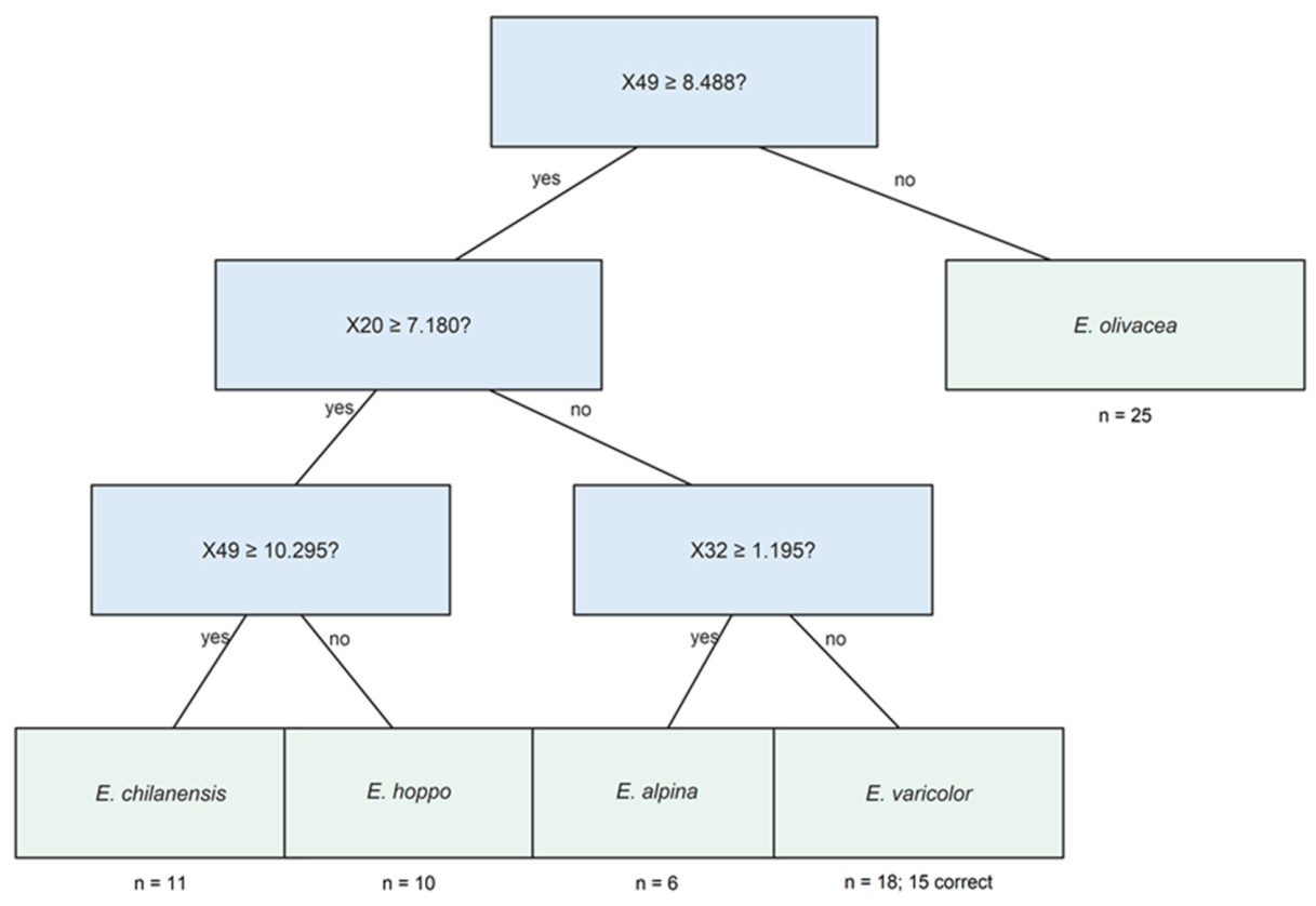
To translate multivariate information into an inspectable decision aid, we fitted CART to the 20 external characters. The tree replaces fixed verbal couplets with measured thresholds and can use different characters on different branches. Tree complexity (cp = 0, 0.001, 0.003, 0.01, 0.03, or 0.05) and minimum split size (4, 6, or 8 specimens) were selected by four-fold inner cross-validation within each partition of the same 20 repeats of five-fold outer resampling. Maximum depth was six. Accuracy and balanced accuracy were calculated only from outer-fold predictions. A final pruned tree fitted to all 70 specimens was exported as a provisional quantitative screening tree (Figure 8), not as an operational taxonomic key or species-delimitation model.
Open-set taxonomic projection
The final classifiers were fitted to all 70 development specimens with the 20 non-destructive characters and weight decay 1, the modal choice in nested resampling. Projection specimens were first evaluated at t = 0.60. Characters were standardized using development-set means and standard deviations. A pooled within-class covariance matrix S was regularized as S<sub>r</sub> = (1 - lambda)S + lambda diag(S), with lambda = 0.5 fixed before projection. This prespecified mid-range shrinkage was retained to stabilize inversion in the small-sample projection analysis and to avoid tuning a rejection rule on the heterogeneous projection set; it is a design choice rather than an estimated optimum. Squared Mahalanobis distance from a specimen to its predicted-class centroid was compared with a single pooled 95th percentile (type-8 quantile) of leave-one-out distances of development specimens from their own leave-one-out class centroids; no class-specific cutoff was used. Acceptance required classifier agreement and a distance below this cutoff. PCA in Figure 7 was calculated from the centred and scaled 20-character development matrix and used only for two-dimensional display.
Leave-one-species-out unknown-class validation
Open-set performance was evaluated separately from the heterogeneous projection specimens. Each reference species was omitted in turn and designated the positive “unknown” class. In each of 20 repeats, the remaining four classes were partitioned into five stratified folds. The multinomial model, empirical class priors, class centroids, pooled covariance, and single pooled 95th-percentile distance cutoff were recalculated independently from each training partition. Each represented specimen was evaluated once in its held-out fold. Each omitted specimen was initially evaluated by all five fold-specific models; to prevent fivefold over-weighting, its five distance-to-cutoff ratios were averaged to one specimen-repeat novelty score, which was rejected when the mean ratio exceeded 1. The mean was prespecified because it retains the magnitude of evidence from every fold model on the common cutoff-normalized scale, whereas majority voting discards magnitude. Because this choice is not unique, a sensitivity analysis repeated unknown rejection using the median ratio and a majority rule requiring rejection by at least three of five fold models. A once-per-repeat model refitted to all four retained species was not mixed into the primary analysis because it would use a different training-set size from the held-out known-specimen evaluation; such a model is better treated as a future deployment model rather than a directly paired validation rule. Each known specimen likewise contributed one specimen-repeat score. Thus, known and unknown specimens had equal biological weight: 20 decisions per specimen across repeats. The omitted/known specimen counts were 11/59, 9/61, 15/55, 25/45 and 10/60 for E. chilanensis, E. alpina, E. varicolor, E. olivacea and E. hoppo, respectively.
The normalized novelty score for AUROC and AUPRC was the squared regularized Mahalanobis distance divided by its fold-specific cutoff; larger values indicated greater evidence for “unknown.” We report unique specimen counts, specimen-repeat counts, effective unknown prevalence, the prevalence-based no-skill AUPRC, unknown rejection, false acceptance, known false rejection, AUROC, AUPRC, empirical open-set accuracy and balanced open-set accuracy. Empirical open-set accuracy weights specimens at their observed prevalence; balanced open-set accuracy is the mean of accepted-and-correct known rate and unknown rejection, giving known and unknown status equal importance. Five hundred stratified specimen-cluster bootstrap replicates resampled known and unknown biological specimens separately while retaining all 20 specimen-repeat decisions for each sampled specimen. This design quantifies omitted-species detection inside the present measurement domain, not unknown genera or new imaging domains (Figure 5; Tables S13, S20, and S22).
Taxonomic interpretation
Predictive membership, morphological diagnosis, species delimitation, and nomenclatural action were treated as distinct steps. Models assessed similarity to reference hypotheses and the reliability of identification decisions. Synonymy and species status additionally required examination of name-bearing types, original descriptions, priority, diagnostic morphology, geographic and acoustic evidence where available, and relevant provisions of zoological nomenclature.
3. Results
Data audit
The 70-specimen development matrix contained no missing values or duplicate specimen identifiers. Reference-class sizes were 11, 9, 15, 25, and 10. Several characters were strongly correlated; X35 and X71 were nearly perfectly inversely correlated, as expected from their definitions. A later 2019 workbook contained the same specimen order and values as the high-precision 2016 development matrix, except that X1 had been rounded to two decimal places. Analyses therefore used the unrounded values.
Out-of-sample classification
Across PAM solutions from two to eight groups, the five-group solution had the highest mean silhouette width (0.274). Under 200 perturbations that independently retained 80% of specimens and 80% of characters, its median adjusted Rand agreement with the full-data solution was 1.000 (95% empirical interval 0.910–1.000; Figure 2). Solutions with three, four, and six to eight groups had lower silhouette widths and lower median stability. The two-group solution also had a median adjusted Rand index of 1.000 but a much lower 2.5th percentile (0.009), indicating occasional collapse under perturbation. These results describe structure in the measured morphospace; they do not assign species rank.
Nested resampling produced 1,400 repeated out-of-fold predictions from 70 biological specimens, which remained the independent clusters for uncertainty estimation. Feature-screened multinomial accuracy was 95.93% (specimen-cluster bootstrap 95% CI 91.36–99.48%) and balanced accuracy was 94.71% (87.90–99.38%). Recalls for E. chilanensis, E. alpina, E. varicolor, E. olivacea, and E. hoppo were 99.5%, 86.7%, 99.3%, 98.0%, and 90.0%, respectively (Figure 3). Errors concentrated between E. alpina and E. varicolor and between E. hoppo and E. chilanensis. These are predictions of unseen measurements from the same incompletely annotated reference domain, not evidence of locality-, sex-, or imaging-domain transfer.
All 20 candidate characters were selected in 94 of 100 outer models. The all-character multinomial model had the highest closed-set accuracy (96.57%, 95% CI 92.21–99.93%) and balanced accuracy (95.41%, 88.60–99.90%), followed by the feature-screened multinomial model (95.93%; 94.71%) and RDA (95.79%; 94.24%). The paired accuracy difference between feature-screened and all-character multinomial models was −0.64 percentage points (95% CI −1.29 to −0.14), confirming that screening did not improve prediction. RDA traded a small, uncertain accuracy difference (−0.79 points, −2.33 to 0.36) for a lower Brier score (difference −0.033, −0.055 to −0.010) and lower ECE (−0.103, −0.124 to −0.075). The ratios-only model achieved 92.93% accuracy, showing that dimensionless shape information remained substantial but did not equal the mixed distance-and-ratio set. Full model estimates, cluster intervals, paired differences, and repeat-level sensitivity appear in Tables S14–S19.
Selective-classification performance
At t = 0.50, 90.71% of predictions were accepted and conditional accuracy was 97.87%. At the illustrative threshold t = 0.60, agreement-rule coverage was 82.00% (specimen-cluster 95% CI 74.64–88.55%) and conditional accuracy was 98.61% (96.16–99.92%; Figure 4). More conservative thresholds increased reliability while sharply reducing coverage. At descriptively matched 82% coverage, conditional accuracy was 99.83% for the all-character multinomial score, 99.39% for RDA, and 98.17% for the feature-screened multinomial score. The agreement rule therefore supplies a transparent disagreement flag but is not the principal performance gain and did not outperform simpler confidence rejection (Tables S15–S19).
Probability calibration
For the feature-screened multinomial component, the multiclass Brier score was 0.100 (specimen-cluster 95% CI 0.054–0.165), mean one-versus-rest Brier score was 0.031 (0.022–0.044), and 10-bin top-label ECE was 0.098 (0.061–0.136; Figure 6; Tables S11, S12, S16, and S21). Five-bin sensitivity analyses led to the same qualitative conclusion. In five equal-width bins, only one unique specimen contributed to the lowest occupied confidence region; equal-frequency bins contained 32–54 unique specimens but the same specimens could contribute to multiple bins across repeats. Calibration is therefore internal and imprecise in sparse low-confidence regions. RDA showed better internal calibration, but the small specimen count precludes treating any score as a universally calibrated probability. Thresholds are decision settings, not taxonomic posterior probabilities.
Leave-one-species-out open-set performance
After aggregation to one decision per specimen per repeat, unknown-class rejection remained strongly taxon dependent (Figure 5; Tables S13, S20, and S22). Rejection was 100% for E. chilanensis (empirical specimen-cluster bootstrap interval 100–100%), 100% for E. olivacea (100–100%) and 92.0% for E. hoppo (76.0–100%). These empirical intervals describe stability under resampling of the finite observed specimens; a 100–100% interval does not imply that the rejection probability for future specimens is necessarily 100%. By contrast, rejection was 21.1% for E. alpina (0–45.5%; false acceptance 78.9%) and 35.0% for E. varicolor (13.2–58.7%; false acceptance 65.0%). Corrected AUPRC values were 0.794, 0.938, 0.709, 0.274 and 0.453 for E. chilanensis, E. olivacea, E. hoppo, E. alpina and E. varicolor, respectively; their no-skill baselines were the effective unknown prevalences 0.157, 0.357, 0.143, 0.129 and 0.214. Balanced open-set accuracies were 0.933, 0.938, 0.892, 0.556 and 0.621, respectively. The wide intervals reflect only 9–25 independent unknown specimens. Equal biological weighting substantially reduced prevalence-sensitive AUPRC estimates but preserved the central conclusion: reference-library absence is detectable when an omitted taxon is separated in measured morphospace and may be invisible when it overlaps represented species. Aggregation-rule sensitivity supported the same conclusion. Mean, median and majority-vote rejection rates were respectively 21.1%, 15.0% and 15.0% for E. alpina; 100%, 99.5% and 99.5% for E. chilanensis; 92.0%, 92.5% and 92.5% for E. hoppo; 100% under all three rules for E. olivacea; and 35.0%, 30.0% and 30.0% for E. varicolor (Table S22). Median and majority voting were identical in point estimates because five fold votes yield an odd decision count; modest mean-versus-median differences did not alter the species ranking or inference.
Projection of taxonomically important material
Sixteen of 55 non-duplicated projection specimens satisfied classifier agreement and the distance criterion; 20 were rejected because component classifiers disagreed and 19 because they exceeded the distance cutoff (Figure 7). Because the leave-one-species-out analysis showed high false acceptance for some omitted species, these projection outcomes are exploratory similarity assessments rather than independent open-set validation. Results are reported with species names in Tables S6 and S7; no synonymy, identification of an unrepresented taxon or nomenclatural conclusion is inferred from an accepted projection.
Performance of the quantitative screening tree
Dedicated nested tuning yielded 80.57% accuracy and 76.61% balanced accuracy (Tables S9 and S10); common benchmark folds gave 82.00% and 78.02%, respectively (Table S14). The final tree contained five terminal leaves and used X49, X20, and X32 (Figure 8). One terminal leaf contained classification errors, and X49 is an unadjusted abdominal distance that can encode size. The tree is therefore a provisional quantitative screening aid, not an operational taxonomic key.
4. Discussion
A taxonomic workflow, not a single winning classifier
The classifier-modelling system is more than a contest for the highest accuracy. Its contribution is an explicit sequence from harmonized character acquisition to leakage-resistant model comparison, abstention, reference-gap testing, interpretable screening, and taxonomic review. Because the models consume defined morphological variables rather than raw pixels, the workflow can support conventional specimen-based taxonomy, image-enabled taxonomy, or a hybrid design combining compatible measurements from specimens, living individuals, and images. Its practical advantage is not the removal of expert judgment but the conversion of part of that judgment into documented variables, fitted thresholds, out-of-sample error estimates, explicit rejection, and a reproducible audit trail. This can prioritize difficult specimens, reduce repetitive screening, expose inconsistent assignments, and reserve destructive or costly follow-up for cases in which it is most informative. External characters retained strong predictive information after every selection decision was restricted to training data. The resulting accuracy concerns unseen measurements from the same incompletely annotated reference domain; that is narrower than geographic transfer, but more informative than resubstitution fit.
No classifier dominated every criterion. The all-character multinomial model maximized closed-set accuracy, RDA provided better Brier score and ECE, and the compound agreement rule offered an intuitively auditable reason for abstention without improving matched-coverage accuracy. This comparison is itself informative: the originality of the system does not depend on a proprietary algorithm. It lies in making taxonomic decisions and their failure modes measurable, exposing when a complex rule adds value and when a simpler model should be preferred.
Reference-library overlap is the critical failure mode
The leave-one-species-out experiment supplies the broadest biological inference. Open-set recognition is often discussed as though “unknown” were an intrinsic detectable state. It is not. A specimen is unknown relative to a library, whereas rejection depends on its position relative to represented morphospace. E. chilanensis, E. hoppo, and E. olivacea produced strong novelty signals when omitted; E. alpina and E. varicolor were usually absorbed by retained classes. High closed-set accuracy can therefore coexist with poor protection against a biologically plausible missing species.
For systematic research, this changes how automated identifications should be interpreted. Acceptance means that a specimen resembles one represented hypothesis under the measured characters; it does not demonstrate reference completeness. Rejection identifies insufficient support for an assignment but does not establish a new species. Reliable deployment requires deliberate “challenge taxa” chosen for morphological proximity, not only random withholding from well-separated classes. This principle applies beyond cicadas to morphometric keys, barcode reference systems, and image classifiers whenever the taxonomic library is incomplete.
Relationship to integrative and iterative taxonomy
Species are hypotheses that remain open to testing by additional evidence [41]. Our workflow contributes a repeatable phenotypic line of evidence; it does not transform a predicted label into a species boundary. This distinction addresses a recurrent difficulty in computational taxonomy, in which identification, clustering, and species delimitation are treated as interchangeable tasks. They are not. A stable cluster can motivate a species hypothesis, a classifier can test diagnosability relative to named references, and an open-set procedure can identify unsupported projections, but formal delimitation must synthesize morphology, types, geography, behavior, genetics when available, and nomenclature.
The history of E. chilanensis illustrates this iterative relationship but is not independent prospective validation. The quantitative work and subsequent description shared a research programme and an author, and the present model uses E. chilanensis as an already labelled class. Chen et al. (2021) is therefore cited as historical context showing compatibility with a later conventional description, not as proof that the present model discovered an unknown species. A genuine reconstruction would require freezing the pre-description data and labels and withholding all information that encoded the later taxonomic hypothesis.
From dichotomous keys to quantitative screening trees
Traditional dichotomous keys remain valuable because their decisions are inspectable and can be followed without specialized software; they remain part of the diagnosis and specimen-determination functions of taxonomy [8]. Their limitations are equally familiar: couplets are fixed by the author, continuous variation must be converted into verbal states, an early error propagates through all later choices, and a missing or damaged character may make the remaining route unusable. A classification tree retains the inspectable branching logic but learns the ordering and thresholds from labelled reference specimens. It can therefore be regenerated when new material is added, tested on specimens withheld from tree construction, and distributed as either a printed diagram or an interactive key.
The present tree should not be advertised as a finished replacement. Hard splits discard information near thresholds, its accuracy was lower than multivariate models, and it has no intrinsic unknown-class mechanism. Its value is as a provisional, updateable screening interface: the tree provides a human-readable route, probabilistic models provide confirmation and abstention, the distance screen challenges reference adequacy, and the taxonomist retains responsibility for diagnosis, types, delimitation, and nomenclature. With larger sex-balanced reference sets, the same architecture could generate quantitatively tested keys whose error is known rather than assumed.
Flexible specimen-, live-individual-, and image-enabled taxonomy
The framework is useful both within conventional collection-based taxonomy and when dissection or destructive sampling is undesirable, because the selected 20 characters can be measured without spreading the wings. Its distinctive advantage is acquisition flexibility: a study can use direct examination or measurement of specimens and living individuals, calibrated image-derived measurements, or a harmonized combination of these sources, according to material availability and the biological question. Unlike calling song and male genitalia, these external measurements are technically available from both sexes. This creates a route toward female identification in a group whose traditional taxonomy is male centred. The present archive cannot quantify female-specific accuracy, so that advantage is methodological capability rather than a completed sex-transfer validation. A targeted female reference series is an immediate and biologically important next test.
Important limitations remain. Direct and image-derived measurements can have different error structures, while photographic optics, perspective, body positioning, preservation, landmark operator, and image resolution can introduce domain shifts. A photograph-only record may be adequate for testing similarity to reference groups yet insufficient for formal description. Future work should therefore quantify repeatability within and among observers and compare compatible measurements obtained directly from living or preserved material with those extracted from living-individual images, freshly prepared specimens, historical specimens, and published plates. Image-derived evidence is best presented as one flexible, potentially non-destructive component of a specimen-based or integrative taxonomic design, not as a universal reason to stop collecting or directly examining specimens.
Taxonomic implications and limits
The projection results do not provide independent support for synonymy. The E. elongata holotype and material historically identified as E. kotoshoensis contributed to reference-class construction, so their subsequent fitted or projected positions partly reproduce supplied labels. These specimens remain relevant to type-based comparison, but nomenclatural conclusions require an explicitly independent revision.
The leave-one-species-out results define a sharper limit. Morphologically separated omissions were usually rejected, whereas most omitted E. alpina and E. varicolor specimens were falsely accepted. Distance rejection can flag some gaps in a reference library, but absence from the library is not identifiable when an unknown overlaps known morphospace. Neither acceptance nor rejection is evidence of species status.
Limitations and future validation
The five reference classes comprise only 70 unequal and predominantly male specimens. Missing locality, session, sex, preservation, and accession fields prevent leave-locality-out, session-blocked, or sex-stratified validation and leave open whether part of the signal reflects population structure, sexual size variation, collection series, or image batches. A prospective repeat-landmarking experiment was not part of the present design, and raw distances were not corrected for allometry. These limitations define the next confirmatory design: prospective specimen metadata, female-rich sampling, independent observers, multiple cameras and collections, and integration with acoustic and molecular evidence.
Computational reproducibility and primary-data access must be distinguished. The supplied archive reproduces every statistical analysis from the processed measurement matrix, including folds, scores, tuning, bootstrap results and figures. The original photographs and landmark-coordinate data are maintained outside the public computational archive and were supplied privately for peer review of the preceding new-species study [36]. They may be requested from the corresponding author through normal academic procedures, subject to collection, copyright and specimen-access conditions. Most voucher and type material remains in the public institutional collections identified above and can be re-examined or remeasured after collection approval, allowing independent reconstruction or replication of the morphometric experiment. The present study did not itself conduct a prospective multi-observer or multi-camera transfer experiment; consequently, observer- and camera-domain transfer remain untested rather than impossible to verify.
5. Conclusions
Harmonized external morphology, acquired from specimen-, living-individual-, and image-associated source material, supported accurate classification within five Euterpnosia reference classes, and abstention made decision reliability explicit. The strongest result, however, was not the 95.93% closed-set accuracy: it was the demonstration that omitted species were rejected only when their measured morphospace separated from represented classes. This exposes a general reference-library failure that accuracy alone cannot reveal. By integrating flexible character acquisition, nested comparison, calibration, abstention, omission stress tests, and an interpretable screening tree, the system provides an original and falsifiable framework for classifier-assisted taxonomy. It can complement traditional specimen research, enable calibrated image analysis, or combine both, provided that definitions, homology, units, and measurement calibration are compatible. The external-character protocol is technically applicable to females because it does not require song or male genitalia, but female identification performance has not yet been evaluated and requires a deliberately female-rich validation set. The archive reproduces the statistical stage from processed measurements. Original images and landmark data are available through academic request, and museum vouchers permit independent remeasurement; however, this study did not prospectively estimate observer-, acquisition-mode-, or camera-domain transfer. Model acceptance supports identification relative to available references; delimitation and nomenclature remain integrative taxonomic decisions.
Supplementary Materials
The following supporting information can be downloaded at the website of this paper posted on Preprints.org. Additional supporting information may be found online in the Supporting Information section at the end of the article. Table S1. Definitions and analytical roles of morphometric characters used in the study. Table S2. Nested cross-validation performance metrics and specimen-cluster bootstrap confidence intervals. Table S3. Accuracy–coverage results across selective-classification thresholds. Table S4. Confusion matrix from repeated nested cross-validation. Table S5. Silhouette width and perturbation stability for alternative numbers of morphological groups. Table S6. Open-set projection results for taxonomically important specimens. Table S7. Summary of projection outcomes by specimen prefix or taxon code. Table S8. Records excluded before analysis because their source labels were explicitly uncertain. Table S9. Nested cross-validation performance of the pruned classification-tree identification key. Table S10. Confusion matrix for nested classification-tree predictions. Table S11. Out-of-fold calibration metrics for the multiclass and one-versus-rest classifiers. Table S12. Ten-bin reliability data for the multiclass classifier. Table S13. Leave-one-species-out open-set performance by omitted species, including resampling intervals. Table S14. Benchmark-model performance evaluated on identical outer-fold assignments. Table S15. Descriptive comparison of benchmark classifiers at approximately matched 82% coverage. Table S16. Specimen-cluster bootstrap confidence intervals for calibration, coverage, and conditional-accuracy metrics. Table S17. Specimen-cluster bootstrap confidence intervals for benchmark-model performance. Table S18. Paired specimen-cluster bootstrap differences between benchmark models. Table S19. Between-repeat sensitivity summaries for benchmark-model performance. Table S20. Equal-weight leave-one-species-out performance with biological specimen counts, specimen-repeat counts, effective prevalence, no-skill AUPRC baselines, and stratified specimen-cluster confidence intervals. Table S21. Calibration sensitivity using five equal-width and five equal-frequency bins, including prediction and unique-specimen counts. Table S22. Leave-one-species-out aggregation sensitivity comparing mean cutoff-normalized distance, median cutoff-normalized distance, and majority rejection across the five fold-specific models, with empirical specimen-cluster bootstrap intervals.
Author Contributions
Conceptualization, T.-Y.H.; methodology, T.-Y.H. and F.L.; software, T.-Y.H.; validation, T.-Y.H. and F.L.; formal analysis, T.-Y.H.; investigation, T.-Y.H.; resources, T.-Y.H. and F.L.; data curation, T.-Y.H.; visualization, T.-Y.H.; writing—original draft preparation, T.-Y.H.; writing—review and editing, T.-Y.H. and F.L. All authors have read and agreed to the submitted version of the manuscript.
Funding
This research received no competitive government or university grant. During 2025–2026, Lanxi Agricultural Technology Co., Ltd., Wuyou Ecological Agriculture Co., Ltd., Cai Die Biological Technology Co., Ltd., and Fujian Tianyuan Shiguang Leisure Agriculture Co., Ltd. provided substantial research support, including experimental space, researcher salaries, cameras and other basic equipment used for analysis and manuscript preparation. These contributions formed part of the research environment that made the work possible and are acknowledged as material institutional support. No grant number applies. The supporting companies had no role in the statistical design, model fitting, interpretation of results, decision to publish, or preparation of the final scientific conclusions.
Data Availability Statement
The original contributions supporting the numerical results are included in the article and Supplementary Materials. The complete computational archive contains the 70-specimen development matrix, projection matrix, exclusion record, 1,400 repeated outer-fold predictions with fold and repeat identifiers, class scores, tuning results, selected variables and hyperparameters, leave-one-species-out decisions, specimen-cluster bootstrap results, benchmark outputs, executable R scripts, random seeds, package information, figures and SHA-256 checksums. Original photographs and landmark-coordinate data were provided privately during peer review of the preceding E. chilanensis new-species publication and are available from the corresponding author upon reasonable academic request, subject to applicable collection and copyright conditions. Most underlying voucher and type specimens remain accessible in the public institutional collections listed in the Methods and may be independently re-examined or remeasured after approval. A versioned Zenodo deposit of the final computational archive will be created upon acceptance and its DOI added to the published Data Availability Statement.
Acknowledgments
We thank C.-H. Chen and Y.-M. Zhang for field assistance, W.-J. Chen for access to specimens, and the curators and staff of NMNS, TFRI, NTU, and SEHU.
Conflicts of Interest
T.-Y.H. and F.L. report employment affiliations during 2025–2026 with Lanxi Agricultural Technology Co., Ltd., Wuyou Ecological Agriculture Co., Ltd., Cai Die Biological Technology Co., Ltd., and Fujian Tianyuan Shiguang Leisure Agriculture Co., Ltd. These research- and technology-oriented companies provided the material support described in the Funding Statement, and their contribution to the research environment is acknowledged. The authors retained scientific responsibility for data analysis, interpretation and preparation of the manuscript. All material support and employment relationships relevant to this study are disclosed. The authors declare no additional competing financial interest, patent or equity interest arising from this work.
References
- Agnarsson, I.; Kuntner, M. Taxonomy in a changing world: Seeking solutions for a science in crisis. Syst. Biol. 2007, 56, 531–539. [CrossRef]
- Löbl, I.; Klausnitzer, B.; Hartmann, M.; Krell, F.-T. The silent extinction of species and taxonomists—An appeal to science policymakers and legislators. Diversity 2023, 15, 1053. [CrossRef]
- Liu, D.; Thompson, J.R.; Gao, J.; Shen, H. Train young scientists in taxonomy to help solve the biodiversity crisis. Nature 2024, 626, 954. [CrossRef]
- Páll-Gergely, B.; Krell, F.-T.; Ábrahám, L.; Bajomi, B.; Balog, L.E.; Boda, P.; Csuzdi, C.; Dányi, L.; Fehér, Z.; Hornok, S.; et al. Identification crisis: A fauna-wide estimate of biodiversity expertise shows massive decline in a Central European country. Biodivers. Conserv. 2024, 33, 3871–3903. [CrossRef]
- Forbes, O.; Young, A.G.; Thrall, P.H. Global sampling decline erodes science potential of natural history collections. Nat. Commun. 2025, 16, 9255. [CrossRef]
- Goodwin, Z.A.; Harris, D.J.; Filer, D.; Wood, J.R.I.; Scotland, R.W. Widespread mistaken identity in tropical plant collections. Curr. Biol. 2015, 25, R1066–R1067. [CrossRef]
- Hollister, J.D.; Martin, G.; Cai, X.; Horton, T.; Powell, O.; Sterling, M.; Turnbull, G.; Price, B.W.; Fenberg, P.B. A computer vision method for finding mislabelled specimens within natural history collections. Ecol. Evol. 2025, 15, e71648. [CrossRef]
- Favret, C. The 5 ‘D’s of taxonomy: A user’s guide. Q. Rev. Biol. 2024, 99, 131–156. [CrossRef]
- Ahrens, D. Species diagnosis and DNA taxonomy. In Species Identification of Insects: Morphological and Molecular Techniques; Humana: New York, NY, USA, 2024; Volume 2744, pp. 33–52. [CrossRef]
- Andersen, J.C.; Mills, N.J. DNA extraction from museum specimens of parasitic Hymenoptera. PLoS ONE 2012, 7, e45549. [CrossRef]
- Santos, D.; Ribeiro, G.C.; Cabral, A.D.; Sperança, M.A. A non-destructive enzymatic method to extract DNA from arthropod specimens. PLoS ONE 2018, 13, e0192200. [CrossRef]
- Brown, M.E.; Ottati, S.; Trivellone, V. A non-destructive, fast, inexpensive, non-toxic chelating resin-based DNA extraction protocol for insect voucher specimens and associated microbiomes. J. Insect Sci. 2025, 25, 17. [CrossRef]
- Tan, Y.; Zhao, Z.; Yuan, X.; Zhao, Y.; Su, D.; Song, Y. Research trends, hotspots and future perspectives of geometric morphometrics in entomology: A scientometric review. Insects 2026, 17, 325. [CrossRef]
- Yang, H.-P.; Ma, C.-S.; Wen, H.; Zhan, Q.-B.; Wang, X.-L. A tool for developing an automatic insect identification system based on wing outlines. Sci. Rep. 2015, 5, 12786. [CrossRef]
- Bellin, N.; Calzolari, M.; Callegari, E.; Bonilauri, P.; Grisendi, A.; Dottori, M.; Rossi, V. Geometric morphometrics and machine learning as tools for the identification of sibling mosquito species of the Maculipennis complex (Anopheles). Infect. Genet. Evol. 2021, 95, 105034. [CrossRef]
- Khang, T.F.; Mohd Puaad, N.A.D.; Teh, S.H.; Mohamed, Z. Random forests for predicting species identity of forensically important blow flies and flesh flies using geometric morphometric data: Proof of concept. J. Forensic Sci. 2021, 66, 960–970. [CrossRef]
- Yeo, H.; Lin, J.; Yeoh, T.X.; Puniamoorthy, N. Resolution of cryptic mosquito species through wing morphometrics. Infect. Genet. Evol. 2024, 123, 105647. [CrossRef]
- Zhang, M.; Du, Y.; Deng, X.; He, J.; Jiang, H.; Liu, Y.; Hao, J.; Chen, P.; Xu, K.; Niu, Q. An XGBoost-based morphometric classification system for automatic subspecies identification of Apis mellifera. Insects 2026, 17, 27. [CrossRef]
- Steinke, D.; Ratnasingham, S.; Agda, J.; Ait Boutou, H.; Box, I.C.H.; Boyle, M.; Chan, D.; Feng, C.; Lowe, S.C.; McKeown, J.T.A.; et al. Towards a taxonomy machine: A training set of 5.6 million arthropod images. Data 2024, 9, 122. [CrossRef]
- Tannous, M.; Stefanini, C.; Romano, D. A deep-learning-based detection approach for the identification of insect species of economic importance. Insects 2023, 14, 148. [CrossRef]
- Huo, H.; Mei, A.; Xu, N. Polymorphic clustering and approximate masking framework for fine-grained insect image classification. Electronics 2024, 13, 1691. [CrossRef]
- Liu, M.; Wang, L.; Jia, R.; Ji, S.; Wu, Y.; Wu, Y.; Xie, L.; Dong, M. Cross-modal and contrastive optimization for explainable multimodal recognition of predatory and parasitic insects. Insects 2025, 16, 1187. [CrossRef]
- Chow, C.K. On optimum recognition error and reject tradeoff. IEEE Trans. Inf. Theory 1970, 16, 41–46. [CrossRef]
- Herbei, R.; Wegkamp, M.H. Classification with reject option. Can. J. Stat. 2006, 34, 709–721. [CrossRef]
- El-Yaniv, R.; Wiener, Y. On the foundations of noise-free selective classification. J. Mach. Learn. Res. 2010, 11, 1605–1641.
- Scheirer, W.J.; Rocha, A.; Sapkota, A.; Boult, T.E. Toward open set recognition. IEEE Trans. Pattern Anal. Mach. Intell. 2013, 35, 1757–1772. [CrossRef]
- Geng, C.; Huang, S.-J.; Chen, S. Recent advances in open set recognition: A survey. IEEE Trans. Pattern Anal. Mach. Intell. 2021, 43, 3614–3631. [CrossRef]
- Friedman, J.H. Regularized discriminant analysis. J. Am. Stat. Assoc. 1989, 84, 165–175. [CrossRef]
- Peng, C.-I.; Hsieh, T.-Y.; Nguyen, Q.H. Begonia kui (sect. Coelocentrum, Begoniaceae), a new species from Vietnam. Bot. Stud. 2007, 48, 127–132.
- Hsieh, T.-Y.; Hsu, T.-C.; Kono, Y.; Ku, S.-M.; Peng, C.-I. Gentiana bambuseti (Gentianaceae), a new species from Taiwan. Bot. Stud. 2007, 48, 349–355.
- Hsieh, T.-Y.; Ku, S.-M.; Chien, C.-T.; Liou, Y.-T. Classifier modeling and numerical taxonomy of Actinidia (Actinidiaceae) in Taiwan. Bot. Stud. 2011, 52, 337–357.
- Hsieh, T.-Y.; Hatch, K.A.; Chang, Y.-M. Phlegmariurus changii (Huperziaceae), a new hanging firmoss from Taiwan. Am. Fern J. 2012, 102, 283–288. [CrossRef]
- Xiao, Y.; Li, C.; Hsieh, T.-Y.; Tian, D.-K.; Zhou, J.-J.; Zhang, D.-G.; Chen, G.-X. Eutrema bulbiferum (Brassicaceae), a new species with bulbils from Hunan, China. Phytotaxa 2015, 219, 233–242. [CrossRef]
- Hsieh, T.-Y.; Chang, C.-R.; Yang, C.-J.; Li, F. Numerical ecology and social network analysis of the forest community in the Lienhuachih area of Taiwan. Diversity 2023, 15, 60. [CrossRef]
- Hsieh, T.-Y.; Li, F.; Huang, S.-L.; Chien, C.-T. Species-specific responses of kiwifruit seed germination to climate change using classifier modeling. Plants 2025, 14, 2665. [CrossRef]
- Chen, J.-H.; Hsieh, T.-Y.; Chen, W.-Z.; Chen, C.-H.; Chang, Y.-M. A new species of the cicada genus Euterpnosia from Taiwan, with morphometric approaches. Formos. Entomol. 2021, 41, 192–207. [CrossRef]
- Ambroise, C.; McLachlan, G.J. Selection bias in gene extraction on the basis of microarray gene-expression data. Proc. Natl. Acad. Sci. USA 2002, 99, 6562–6566. [CrossRef]
- Vabalas, A.; Gowen, E.; Poliakoff, E.; Casson, A.J. Machine learning algorithm validation with a limited sample size. PLoS ONE 2019, 14, e0224365. [CrossRef]
- Gneiting, T.; Raftery, A.E. Strictly proper scoring rules, prediction, and estimation. J. Am. Stat. Assoc. 2007, 102, 359–378. [CrossRef]
- Guo, C.; Pleiss, G.; Sun, Y.; Weinberger, K.Q. On calibration of modern neural networks. In Proceedings of the 34th International Conference on Machine Learning, Sydney, Australia, 6–11 August 2017; Volume 70, pp. 1321–1330.
- Yeates, D.K.; Seago, A.; Nelson, L.; Cameron, S.L.; Joseph, L.; Trueman, J.W.H. Integrative taxonomy, or iterative taxonomy? Syst. Entomol. 2011, 36, 209–217. [CrossRef]
Figure 1.
Anatomical landmarks used for Euterpnosia morphometrics. (A) Forewing landmarks 1–30, shown as open red circles; these require a spread-wing image. (B) Abdominal landmarks 43–68 and 73–84, shown as solid red circles. (C) Head-and-thorax landmarks 31–42 and 69–72; cyan numerals distinguish the central head-and-thorax series from the red peripheral points. Characters X20–X35, X49, X50, X70 and X71 can be measured without spreading the wings; complete definitions are provided in Table S1.
Figure 1.
Anatomical landmarks used for Euterpnosia morphometrics. (A) Forewing landmarks 1–30, shown as open red circles; these require a spread-wing image. (B) Abdominal landmarks 43–68 and 73–84, shown as solid red circles. (C) Head-and-thorax landmarks 31–42 and 69–72; cyan numerals distinguish the central head-and-thorax series from the red peripheral points. Characters X20–X35, X49, X50, X70 and X71 can be measured without spreading the wings; complete definitions are provided in Table S1.
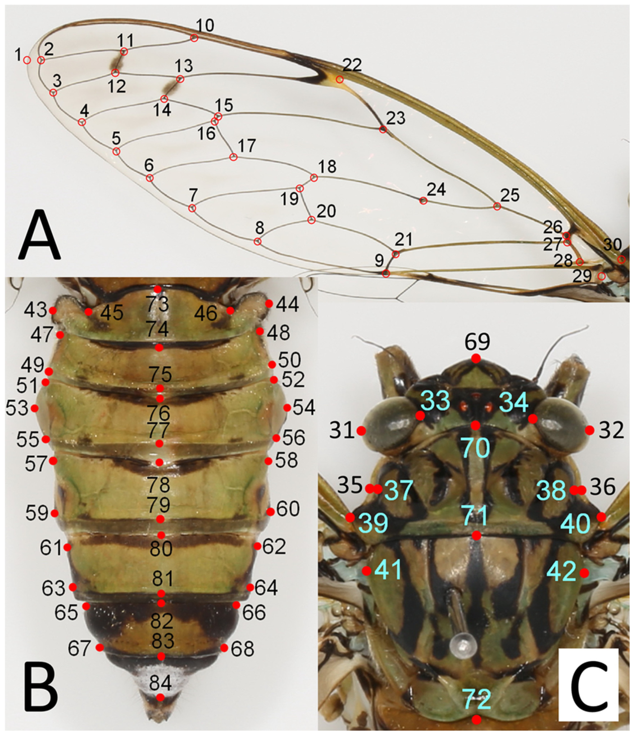
Figure 2.
Selection and perturbation stability of morphological groups. (a) Mean silhouette width for PAM solutions with k = 2–8. (b) Median adjusted Rand index and 2.5–97.5% perturbation interval from 200 iterations retaining 80% of specimens and 80% of characters. The display describes clustering stability and does not delimit species.
Figure 2.
Selection and perturbation stability of morphological groups. (a) Mean silhouette width for PAM solutions with k = 2–8. (b) Median adjusted Rand index and 2.5–97.5% perturbation interval from 200 iterations retaining 80% of specimens and 80% of characters. The display describes clustering stability and does not delimit species.
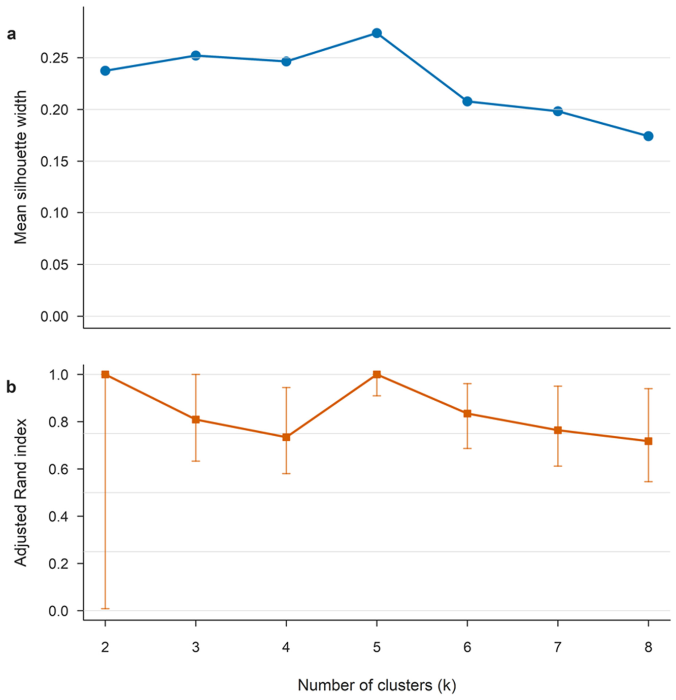
Figure 3.
Confusion matrix from 20 × five-fold nested cross-validation. Rows are named operational reference classes and columns are out-of-sample predictions. Counts aggregate repeated predictions and percentages are row-normalized recalls.
Figure 3.
Confusion matrix from 20 × five-fold nested cross-validation. Rows are named operational reference classes and columns are out-of-sample predictions. Counts aggregate repeated predictions and percentages are row-normalized recalls.
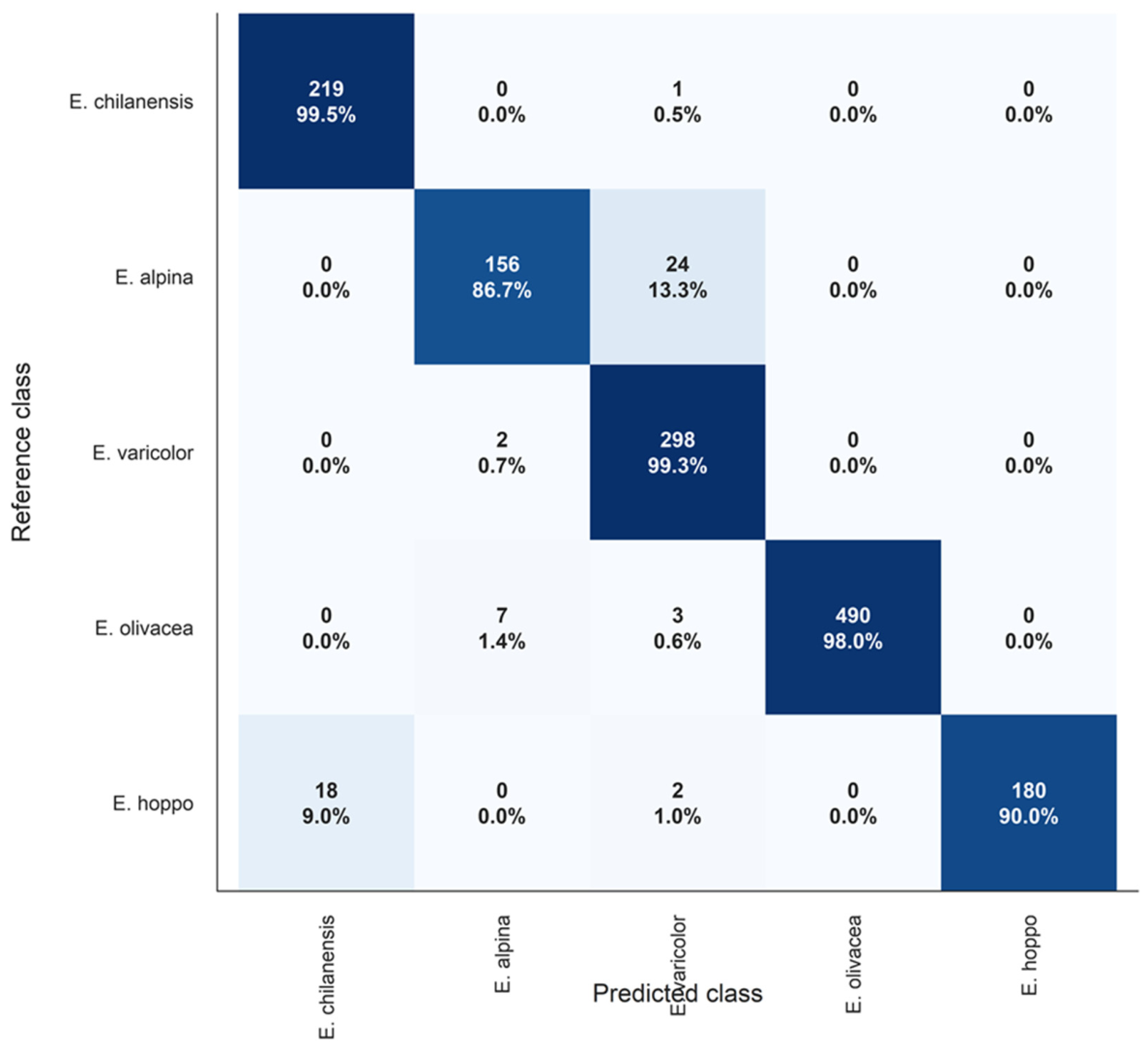
Figure 4.
Accuracy–coverage trade-off for the agreement rule. Points show thresholds from 0.50 to 0.95; ribbons show specimen-cluster bootstrap 95% intervals. The y-axis begins at 0.94 to display the full observed conditional-accuracy range without implying large absolute differences. Threshold 0.60 is illustrative and was not independently prespecified.
Figure 4.
Accuracy–coverage trade-off for the agreement rule. Points show thresholds from 0.50 to 0.95; ribbons show specimen-cluster bootstrap 95% intervals. The y-axis begins at 0.94 to display the full observed conditional-accuracy range without implying large absolute differences. Threshold 0.60 is illustrative and was not independently prespecified.
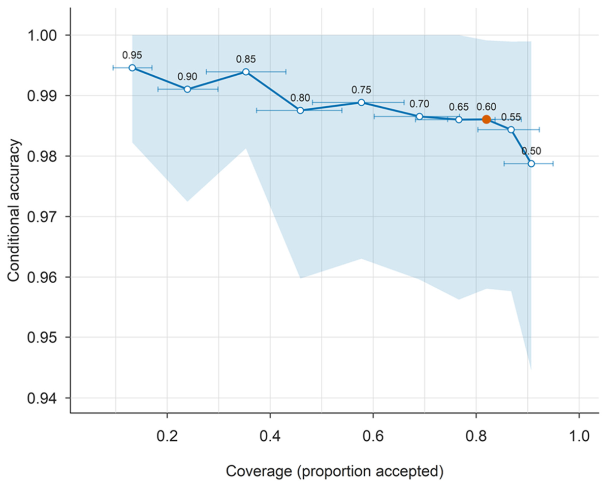
Figure 5.
Leave-one-species-out evaluation of the distance-based unknown-class screen. Points and intervals show equal-biological-weight estimates and empirical specimen-cluster bootstrap intervals for unknown-class rejection and AUPRC when each named species was omitted completely from model development. Performance varies markedly among omitted species.
Figure 5.
Leave-one-species-out evaluation of the distance-based unknown-class screen. Points and intervals show equal-biological-weight estimates and empirical specimen-cluster bootstrap intervals for unknown-class rejection and AUPRC when each named species was omitted completely from model development. Performance varies markedly among omitted species.
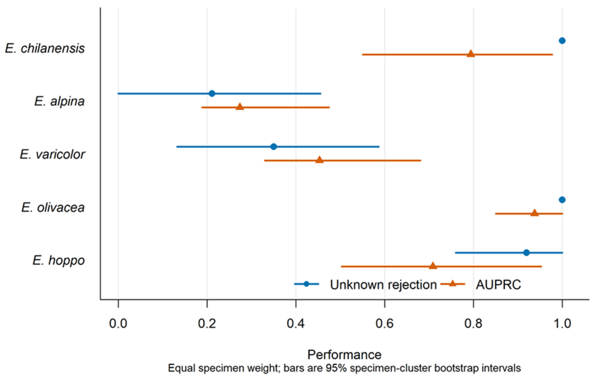
Figure 6.
Out-of-fold reliability of the multiclass classifier. Observed accuracy is plotted against mean predicted confidence in 10 equal-width bins; the diagonal denotes perfect calibration. Brier score and expected calibration error summarize deviations.
Figure 6.
Out-of-fold reliability of the multiclass classifier. Observed accuracy is plotted against mean predicted confidence in 10 equal-width bins; the diagonal denotes perfect calibration. Brier score and expected calibration error summarize deviations.
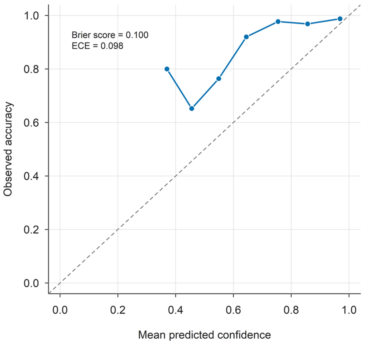
Figure 7.
PCA display of development and taxonomic-projection specimens. Filled translucent circles are development specimens coloured by named reference class. Projected specimens are distinguished by outlined circles (accepted), triangles (classifier disagreement) and crosses (distance rejection). PCA is used only for visualization and is not evidence of open-set performance.
Figure 7.
PCA display of development and taxonomic-projection specimens. Filled translucent circles are development specimens coloured by named reference class. Projected specimens are distinguished by outlined circles (accepted), triangles (classifier disagreement) and crosses (distance rejection). PCA is used only for visualization and is not evidence of open-set performance.
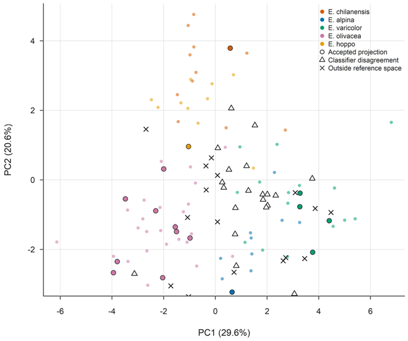
Figure 8.
Provisional quantitative screening tree for the five operational Euterpnosia reference classes. Internal nodes show measured thresholds; terminal nodes show the first-pass classification and development-sample count. The tree is an interpretable screening aid rather than an operational taxonomic key, open-set model, or species-delimitation method.
Figure 8.
Provisional quantitative screening tree for the five operational Euterpnosia reference classes. Internal nodes show measured thresholds; terminal nodes show the first-pass classification and development-sample count. The tree is an interpretable screening aid rather than an operational taxonomic key, open-set model, or species-delimitation method.
Disclaimer/Publisher’s Note: The statements, opinions and data contained in all publications are solely those of the individual author(s) and contributor(s) and not of MDPI and/or the editor(s). MDPI and/or the editor(s) disclaim responsibility for any injury to people or property resulting from any ideas, methods, instructions or products referred to in the content. |
© 2026 by the authors. Licensee MDPI, Basel, Switzerland. This article is an open access article distributed under the terms and conditions of the Creative Commons Attribution (CC BY) license (http://creativecommons.org/licenses/by/4.0/).
Copyright: This open access article is published under a Creative Commons CC BY 4.0 license, which permit the free download, distribution, and reuse, provided that the author and preprint are cited in any reuse.