

Submitted:
23 July 2026
Posted:
24 July 2026
You are already at the latest version
Abstract
Configurable intelligent design is formalized here as the selection of a consistent configuration from interdependent alternatives under strict constraints of budget, quality, risk, and compatibility. Locally correct predictions for individual components do not guarantee a globally feasible solution. The objective of this study is to quantify the differences among direct neural network inference, the exact deterministic HIM-D solver, and a procedural hybrid architecture in which a neural network proposes a candidate, an independent verifier checks all constraints, and control is transferred to an exact search whenever at least one condition is violated. For the experiment, a reproducible synthetic corpus of 24,000 configuration problems spanning educational, engineering, and commercial scenarios was generated. Feasibility of solutions, joint feasibility and optimality, robustness to distribution shift, repeatability, and computational latency were assessed. Pure neural network models achieved feasible solutions in only 17.40% and 19.12% of cases and showed pronounced degradation under out-of-distribution (OOD) conditions. The procedural hybrid maintained 100% feasibility and achieved 83.08% on the composite feasibility-and-optimality metric. These results confirm the effectiveness of architecturally separating probabilistic prediction from independent formal verification when solving configuration problems with tight constraints.
Keywords:
configurational AI architectures
; hierarchical imitation models
; constraint satisfaction problems
; combinatorial optimization
; formal verification
; hybrid artificial intelligence
; out-of-distribution generalization
; reproducible experiment
1. Introduction
Artificial intelligence systems are increasingly used to select educational content, engineering components, production modes, and commercial offers. In all of these cases, the final output is not a single prediction but a coordinated configuration of several interdependent elements. Such a configuration must simultaneously satisfy user preferences, numerical thresholds, logical dependencies, object compatibility, and an optimality criterion. A substantively convincing answer may remain practically unacceptable if even one mandatory condition is violated. The evaluation of such systems therefore cannot be limited to average accuracy or semantic similarity; it requires independent validation, quantitative assessment of deviations from the optimum, robustness analysis under new combinations of conditions, and a reproducible decision-making log.
In [1], an architecture for configurable intelligent design based on hierarchical imitation models (HIM) was proposed as a deterministic alternative to neural-network machine learning for domains in which correctness, transparency, and personalization of results are prioritized. The configurable object was represented as a vector of variables, constraints were defined by a system of functionals, and a library of reference models was intended to be updated through controlled user interaction. Step-by-step validation, computational-complexity management, and an iterative cycle of model testing, tuning, and modification were also proposed.
The scientific value of that original work lay in its comprehensive description of the architecture and methodology; however, its evidence base remained largely conceptual. A large, independent corpus of problems, predefined metrics, interval estimates, a separate generalization test outside the training distribution, and a comparison with direct neural-network solvers were not presented. This gap connects to a broader issue at the intersection of configuration, combinatorial optimization, and machine learning. Classical work treats configuration as a search for a consistent set of components in a finite space under a system of constraints [2,3]. Modern reviews show that machine learning can either strengthen a formal solver or attempt to replace it with a fast predictor [4,5]. The latter approach reduces latency but, without a dedicated verification mechanism, does not guarantee feasibility. A similar gap is observed in research on language models for optimization: a high-quality problem formulation or objective function does not eliminate constraint violations [6,7,8,9].
The objective of this paper is to quantitatively test the architectural principle of separation of concerns, whereby a probabilistic module generates a candidate and a formal module is responsible for the properties that require guarantees. Importantly, this work does not pose the trivial task of proving the superiority of exhaustive search over an approximator: in the chosen problem space, HIM-D is an exact solver and a reference upper bound. The substantive question is to measure the proportion of infeasible direct neural-network outputs, their sensitivity to OOD shift, and the extent to which independent verification with conditional backup search changes robustness, optimality, and latency. To this end, a fixed generator, a single corpus, predefined metrics, paired analysis, a separate OOD test, and an explicit solution-path log are used. The published results of ConstraintBench [6] are reported only as an external benchmark and are not combined with the internal experiment.
The study is organized around four research questions. RQ1: Does HIM-D provide a higher feasibility rate than pure neural network models? RQ2: Does this advantage persist under controlled distribution shift? RQ3: Does hybrid architecture combine neural-network flexibility with a formal feasibility guarantee? RQ4: What is the relationship between robustness gain, objective-function quality, and computational latency?
The scientific novelty of this study lies in translating the conceptual provisions of the original architecture into measurable variables within a single, reproducible experiment: a fully deterministic and testable implementation of HIM-D was formalized; a corpus of 24,000 tasks with separate OOD testing was constructed; a uniform comparison of the deterministic, neural-network, and hybrid approaches was conducted with paired statistical analysis; an external comparison with published results for language models on ConstraintBench was performed; and a reproducibility package with an operational description of the testing pipeline was prepared. Table 1 summarizes the transition from these conceptual provisions to the specific operationalizations, and metrics used in Section 4 and Section 5.
2. Theoretical Foundations and Targeted Analysis of the Literature
2.1. Configuration as a Constraint Satisfaction and Optimization Problem
Configuration design has historically been defined not as the free generation of a new object but as the selection and coordination of elements from predefined families. In the classical formulation, components must be selected, assigned to functions, and connected through admissible relationships so that the resulting system satisfies user requirements and domain rules [2]. A review of industrial configurators shows that the most stable concepts separate domain knowledge-components, resources, and compatibility rules-from the search procedure [3]. This line of research corresponds directly to the class of problems considered here: five decisions are made jointly, and correctness is determined not by the quality of individual choices but by the consistency of the complete set.
Formally, such a problem is close to a finite constraint satisfaction problem with an objective function. Constraint-programming, SAT, mixed-integer-programming methods, and their hybrids can guarantee feasibility and, upon exact search termination, global optimality. The modern CP-SAT-LP solver combines lazy constraint generation, SAT search, linear programming, and a portfolio of strategies [13]. The strength of exact methods lies in the verifiability of the result and the availability of a certificate of search completion; their weakness is that solution time can grow rapidly as the number of variables, variants, and relationships increases.
The hierarchical imitation model HIM-D adheres to this formal tradition but organizes knowledge across the levels of domain, solution group, case, and constraint functional. In this study, the hierarchy is not used as a heuristic guarantee of scalability; rather, it serves as a schema for representing, logging, and reusing rules, while correctness is ensured by exhaustive search over a space of 1024 configurations. Consequently, the 100% feasibility of HIM-D is an expected property of an exact algorithm operating in a small finite space, not empirical evidence of universal superiority.
2.2. Machine Learning for Combinatorial Optimization: Two Distinct Modes
The review by Bengio, Lodi, and Prouvost [4] draws a fundamental distinction. Machine learning can, first, improve individual decisions within a classical algorithm-such as branching, bound estimation, space reduction, or warm-start generation. Second, a model can attempt to map a problem instance directly onto a complete solution. A review of graph neural methods [5] develops this typology further and shows that relational representations are useful for problems in which the input structure is defined by a graph of variables and constraints.
The solver-boosting mode preserves the formal kernel: an error in a trained component typically degrades the speed or quality of the heuristic but does not necessarily render the final solution infeasible, provided full validation is performed before output. A direct neural-network solver operates differently-it produces a solution in one or more passes and can be very fast, but its output is a statistical prediction. Even when each component classification has high local accuracy, the joint solution may violate the global budget, the minimum quality, the risk limit, or at least one compatibility pair.
For tabular and structured data, strong baseline models include residual multilayer networks and attention architectures [11,12]. These are appropriate for testing how well a neural network can recover an optimal configuration from a fixed numerical representation. However, neither the MLP nor the attention architecture inherently encodes the condition “exactly one option from each group, with all pairs compatible.” In the present experiment, pure neural-network models are deliberately evaluated without corrective post-processing. This is not an attempt to present them as the best possible neural optimization method, but a controlled test of the risk inherent in direct inference without a formal verification layer.
This motivates a methodological comparison criterion. For a direct solver, reporting average accuracy for individual groups is insufficient; it is necessary to measure full configuration feasibility, the quality of the objective function among feasible solutions only, the proportion of exact optima, OOD degradation, and the types of simultaneous violations. These are the metrics used below.
2.3. Differentiable Optimization and Hard-Constraint Enforcement
Between the pure predictor and the external exact solver lies a broad class of integrated methods. OptNet incorporates quadratic optimization as a differentiable layer of a neural network [21]. Differentiating through a black-box combinatorial solver allows a model to be trained on final solution quality without replacing the discrete algorithm itself with a continuous approximation [22]. CombOptNet extends this idea to integer programs and allows the objective-function coefficients and constraints themselves to be learned [23]. The shared strength of these approaches is that the solution structure participates in learning rather than being considered only after prediction.
Another line of research builds admissibility into the design. Homeomorphic projection maps the neural-network output onto a feasible set for a wide class of compact sets [24]. LinSATNet introduces a differentiable, positive linear constraint-satisfaction layer and demonstrates it in routing, graph matching, and portfolio problems [25]. HardNet applies a differentiable projection for affine and convex constraints while preserving universal approximation power within the claimed class [26]. These results show that the claim “a neural network inevitably violates constraints” is too strong: constraints can be built into the architecture, but the resulting guarantee depends on their mathematical class and on the completeness of the projection layer.
For the configuration problem considered here, the constraints are heterogeneous: budget, quality, and risk are additive thresholds; the choice of one option from a group is a discrete condition; and compatibility is defined by arbitrary binary relations between groups. Positive linear layers can encode part of this structure, but an arbitrary incompatibility matrix together with the global-minimum requirement preserves the discrete combinatorial component. For this reason, the present study relies on an independent, complete verifier and an exact backup search rather than on a differentiable projection layer.
A further distinction concerns soft versus hard constraints. Adding a violation penalty to the loss function can increase average feasibility, but the resulting penalty does not guarantee feasibility of any single probabilistic output. In applications governed by mandatory rules, correctness must follow either from the design itself or from full verification prior to issuance of the result. This distinction is central to the interpretation of the results below.
2.4. Hybrid and Neuro-Symbolic Systems with Independent Verification
Hybrid artificial intelligence combines learnable and symbolic components, but the mere presence of two module types does not by itself determine reliability. What matters is the computational contract: which module has the authority to produce the final answer, which module checks the constraints, and what happens when a violation is detected. In high-risk tasks, internally interpretable rules and verifiable decisions are preferable to post-hoc explanations of black-box outputs [10]. System context also matters, since hidden dependencies on data, versions, and implicit transformations create technical debt [14].
In the hybrid architecture studied here, the neural network neither modifies the rules nor validates its own decision; its role is limited to proposing a candidate. The verifier recomputes all aggregates and checks all ten intergroup relations. If the candidate is acceptable, it may be adopted as a fast-route solution; if a violation is detected, control is transferred to the exact HIM-D solver. This scheme constitutes a procedural hybrid with conditional control transfer, rather than a jointly trained neuro-symbolic model.
The guarantee here is conditional and must be stated precisely. Final validity reaches 100% only if (i) the verifier implements all mandatory rules, (ii) the input data contain no hidden errors, (iii) the backup solver finds a valid solution, and (iv) no unverified result bypasses the formal route. The log must therefore record the rule version, input parameters, candidate violations, whether the backup solver was invoked, and the final configuration. These documentation principles are consistent with established model-card practice [15].
The hybrid route creates a measurable trade-off. The higher the feasibility of the neural-network candidate, the less frequently the expensive solver is invoked. If a feasible candidate is accepted without an optimality check, speed may improve at the cost of a non-zero objective gap. It is therefore necessary to report, for any hybrid system, the proportion of backup-solver invocations together with final feasibility, joint optimality, and latency.
2.5. Large Language Models: Formulation, Solution, and Tool Use
The literature on large language models (LLMs) and optimization spans several tasks that should not be conflated. The first task is to transform a natural-language description into a mathematical model and solver code. OptiMUS uses a modular LLM agent to formulate mixed-integer problems, generate code, debug it, and verify the solution with an external solver [9]. OptiBench evaluates the full path from a text description to a numerical answer by invoking a software solver [8]. In these systems, the LLM is valuable as an interface and formalizer, while the guarantee of final optimality comes from the external tool.
The second task is direct solution without a formal tool. LR²Bench demonstrates the difficulty of long-chain reflective reasoning on constraint satisfaction problems [7]. ConstraintBench separates formulation from direct search: the model receives a fully specified problem, returns a structured solution, and an independent deterministic verifier checks each condition and compares the objective with the optimum [6]. In this mode, the binding constraint proved to be admissibility itself, rather than objective quality among already-admissible answers.
These results support the functional separation adopted in the present paper. A language or neural-network model can interpret requirements, rank options, and generate a candidate; however, when mandatory discrete rules are present, the final decision must pass through a verifier- or solver-backed route. External LLM metrics are not treated further as a direct experimental competitor to HIM-D, since the problem sets, models, search budgets, and computational environments differ.
2.6. Targeted Literature Synthesis and Research Gap
A targeted analysis of the sources reveals not a single linear scale of methods but six distinct architectural modes. These differ in where the formal structure resides, what is being learned, and at what stage the guarantee arises. Table 2 links these modes to the design of the present experiment.
As the last row of Table 2 indicates, the procedural hybrid is the specific architectural mode this paper tests; the other five rows situate it relative to the alternatives already covered by the literature. The reviewed body of work remains insufficiently focused on how reliability changes when moving from a direct neural-network candidate to independent verification with a conditional exact backup, evaluated on the same set of configuration problems. Work on differentiable optimization offers closer integration, while LLM benchmarks evaluate a different type of input. This study addresses a narrower but operationally clear gap: on a fixed 5×4 framework, it quantitatively compares direct inference, exact solution, and a procedural hybrid in terms of full feasibility, joint optimality, OOD stability, repeatability, and latency.
This formulation also bounds the scientific claims of the study. The work does not claim that brute-force search is a scalable solution, nor does it compare all modern constraint-aware architectures. Its contribution lies in reproducibly measuring the architectural effect of constraint checking and in preparing a baseline for subsequent comparison with CP-SAT, MILP, LinSATNet, projection layers, and solver-in-the-loop learning.
2.7. Implications of the Review for the Experimental Protocol
Five experimental requirements emerge from the literature review. First, the unit of analysis must be a complete configuration, not a single component. Second, validity must be verified independently of the source data used to train the models. Third, objective quality must be assessed separately from validity. Fourth, the ID and OOD sets must be separated in advance. Fifth, the hybrid route and the proportion of backup-solver invocations must be reproducible. These requirements shape the formal model, the corpus description, and the metrics defined in the following sections.
The neural-network results reported below should be interpreted as a baseline for direct forward inference, not as an upper bound for modern neural optimization more broadly. This caveat is important for correctly positioning the article within the target Q1 journal and for preventing unwarranted generalization from two compact networks to the entire class of learning-based methods.
3. Formal Model and Research Hypotheses
3.1. Representation of the Configuration Task
Let u denote a requirements vector and x = (x1, …, xG) a configuration, where each variable xg selects one of O options in group g. In the experiment, G = 5 and O = 4. For each configuration, the cost C(x), quality Q(x), risk R(x), preference-mismatch penalty P(x), and pairwise compatibility matrix K(x) are given. A configuration is feasible when it satisfies the following conditions:
Here Zg,v is a binary indicator for the choice of option v in group g. The objective function combines cost, preference discrepancy, risk, and quality, with coefficients fixed prior to the analysis of the test samples:
The HIM-D implementation searches the finite space of 1024 configurations, eliminates variants that violate at least one hard constraint, and returns a feasible configuration with minimal J(x). In this setting, HIM-D is an exact solver and a computational benchmark, so its 100% feasibility and agreement with the global minimum follow directly from the algorithm's definition when correctly implemented. The substantive experimental question therefore concerns direct neural-network candidates and the effect of independent verification with conditional redundancy. This design establishes a reference upper bound within the controlled space but does not, by itself, demonstrate the scalability of exhaustive search.
3.2. Hypotheses
The hypothesis thresholds were chosen as conservative, practically meaningful boundaries rather than as post hoc choices. The 5-percentage-point margin for H1 and the 1-percentage-point margin for H4 are, respectively, clearly larger than the width of the Wilson 95% confidence intervals for n = 6000 (Section 4.6), allowing a meaningful effect to be distinguished from random variation; this non-inferiority framing follows established equivalence-testing methodology [18]. The latency threshold of under 1 ms per task in H5 reflects the upper bound acceptable for interactive use in the experiment's computing environment.
- H1. The admissibility of HIM-D exceeds the admissibility of each pure neural-network model by at least 5 percentage points.
- H2. The decline in admissibility when moving from ID to OOD conditions is smaller for HIM-D than for each pure neural-network model.
- H3. HIM-D exhibits higher exact repeatability across five runs than stochastic sampling from the neural-network output distributions.
- H4. The hybrid system is not inferior to HIM-D in admissibility, within a 1-percentage-point margin.
- H5. The hybrid system improves joint feasibility and optimality relative to the pure attention network while maintaining sub-1-ms latency per task in the given computing environment.
4. Materials and Methods
4.1. Research Design and Corpus Formation
The study was conducted as a reproducible computational experiment with a pre-fixed generator and an unchangeable evaluation protocol. The corpus contains no personally identifiable information and is not linked to real users, training platforms, production catalogs, or commercial transactions. A total of 24,000 independent numerical instances of a single configuration task were generated: 15,000 instances were used for training, 3,000 for tuning and model-state selection, and 6,000 for final evaluation. The test corpus was pre-partitioned into 3,000 tasks within the training distribution (ID) and 3,000 tasks under a controlled distribution shift (OOD). Numerical instances were distributed equally across the three domain parameterizations and the twelve semantic scenarios described below. Table 3 reports the resulting corpus composition, cross-tabulating each split (training, validation, ID test, and OOD test) against the three domains; it makes explicit how the 24,000 instances decompose into the 15,000/3,000/3,000/3,000 split referenced throughout Section 4 and the 6,000-instance test set analyzed in Section 5.
4.2. Task Generator
Each numerical instance comprised five component groups, each requiring the choice of one of four alternatives. Every alternative was described by continuous indicators of cost, quality, risk, and a penalty for non-compliance with preferences, and a symmetric compatibility matrix was formed for options belonging to different groups. To guarantee the feasibility of each instance, the generator first created a reference feasible configuration, preserved the compatibility of its pairs, and then set budget, quality, and risk thresholds relative to the reference sums. After generation, all 1024 possible configurations were checked with an exhaustive benchmark algorithm; instances for which the existence of a feasible solution could not be confirmed were automatically regenerated.
The three domain parameterizations differed in attribute ranges and in the relative importance of criteria: in the educational parameterization, material quality received increased weight; in the engineering parameterization, cost and risk did; and in the commercial parameterization, price and preference compliance did. The OOD component was formed through three simultaneous modifications: increasing the incompatibility density from 5–13% to 16–28%, narrowing the permissible threshold intervals, and shifting the cost and risk ranges. The OOD problems therefore retained proven solvability but had a smaller admissible domain. It should be emphasized that the subject-area names do not represent real data; they define the interpretation of groups and criteria, while all statistical results refer to synthetic numerical instances.
4.2.1. Unit of Analysis and a Representative Test Task
The unit of analysis is a single, fully specified configuration instance. It is not a textual question and does not require the model to engage in open-ended dialogue; rather, it is a machine-readable task requiring the assembly of one solution from five interdependent choices. This formulation allows the ability to satisfy constraints to be separated from the ability to understand natural language.
- Input. Twenty alternatives organized into five groups of four options. For each alternative, cost, quality, risk, and a preference-mismatch penalty are specified. In addition, three global thresholds, a problem domain, and binary compatibility criteria are specified for all ten pairs of groups.
- Solution. A vector x = (x1, …, x5), where xg indicates the option selected in group g; the complete answer therefore contains exactly five indices.
- Hard constraints. Exactly one option is selected from each group; total cost does not exceed the budget; total quality is not below the minimum; total risk does not exceed the limit; and each of the ten intergroup pairs is compatible.
- Objective. Among feasible configurations, J(x) is minimized, combining cost, preference penalty, risk, and quality with pre-fixed coefficients.
- Benchmark. All 1024 combinations are checked by exhaustive search. For each problem, the existence of a feasible solution, the minimum value J*, and the optimal configuration are recorded.
- Success criteria. Primary success equals one only if all hard constraints are satisfied. Secondary success additionally requires a relative objective gap no greater than 0.1%.
The experiment therefore tests not knowledge of a specific course, device, or product, but the method's ability to generate a globally consistent combination within a limited feasible domain. The subject-specific scenarios define the meaning of the variables and allow the architecture's robustness to be assessed across three numerical parameterizations.
4.2.2. Compact Description of the Twelve Subject Scenarios
Each of the three parameterizations is associated with four scenarios. Each scenario contains 2,000 instances: 1,250 training, 250 validation, 250 ID tests, and 250 OOD-test. The mathematical structure is identical across scenarios, but the substantive interpretation of the five groups and the meaning of the constraints differ. Table 4 allows the reader to see at a glance what exactly is being configured in each case.
Three examples illustrate how to read the table. In E1, a combination in which the explanation method, worked example, and assessment are pitched at different expertise levels, or that exceeds the available time, is unacceptable. In I1, a candidate may satisfy the price and quality criteria yet be rejected because the controller, communication channel, and power supply are incompatible. In C3, a formally attractive plan is rejected if the number of users, security mode, and support tier do not form a valid package.
The scenarios are a semantic shell over a common numerical structure. The generator modifies distributions at the level of the three domains but does not draw on real catalogs or simulate a separate empirical distribution for each scenario. The results therefore pertain to the architectural validation of configuration solutions rather than to demonstrate effectiveness for specific lessons, devices, or products.
4.2.3. Controlled Complexity and Formation of the OOD Shift
The OOD partition was formed by simultaneously changing three factors: increasing the density of incompatibility, narrowing the permissible threshold intervals, and shifting the cost and risk ranges. Each OOD problem retained proven solvability, but the proportion of admissible configurations decreased. This design tests robustness to a more stringent combination of already-known conditions, rather than the emergence of entirely new variable types.
Table 5 lists the six generation factors that jointly define task difficulty and show, factor by factor, how each one moves between the ID and OOD levels; the last column states why each factor was included in the experimental design.
Together, the three tightened thresholds and the higher incompatibility density in Table 5 explain why OOD admissibility is lower than ID admissibility for every system evaluated in Section 5.3, even though the underlying task family and the number of groups and options per group are unchanged.
4.3. Compared Systems
All systems received an identical machine-readable description of the problem. Pure neural-network models generated five probability distributions and independently selected one option per group via argmax; they received no feedback from the verifier and were evaluated without corrective post-processing, so they represent a baseline of forward inference rather than the full spectrum of constraint-aware neural optimization. HIM-D performed exact search and served as the formal reference. The hybrid system used the same attention network but added two untrainable components: an independent verifier and a backup HIM-D solver. Hybridity was implemented at the level of the computational flow rather than through parameter sharing or joint training.
The neural-network candidate is denoted = Nθ(u); the independent test is V(u, x) ∈ {0, 1}; and the exact deterministic solver is S(u) = argmin J(x) over the set of all admissible configurations. The final hybrid operator is defined by the following rule:
(3)
The algorithm proceeds in six steps: (1) the attention network receives the full vector of attributes, thresholds, and compatibility relations; (2) a candidate is formed from five options by maximum likelihood; (3) the verifier recomputes cost, quality, risk, and all ten pairwise compatibility relations without using the neural network's probabilities; (4) a feasible candidate is accepted without re-optimization, so it can be feasible without being globally optimal; (5) if at least one condition is violated, a full enumeration of the 1024 configurations is launched and the feasible configuration with minimal J(x) is selected; and (6) the final result is rechecked and logged together with the route taken, the list of violations (if any), and the rule version. This conditional switch between a probabilistic proposal and a formal solution constitutes the hybridity of the system studied here.
Table 6 summarizes the four systems compared in Section 5 side by side-their internal mechanisms, the number of trainable parameters, the scope of the examination each output undergoes before being returned, and each system's role in testing the study's hypotheses.
The parameter counts in Table 6 (471,572 for the Residual MLP versus 10,596 for the attention network) recur in Table 13, where they are related to the measured latency of each system; the "examination restrictions" column anticipates the central empirical contrast of Section 5, between systems whose output is never checked and the hybrid, whose output is always checked before issuance.
4.4. Feature Preparation and Training
The input to each task was represented as five group tokens, each containing 87 features: 16 normalized attributes for the four variants within its own group, 64 binary compatibility features with the four other groups, three global thresholds, a three-component domain indicator, and the incompatibility density. The MLP received a flat vector of 435 features. The attention network processed five tokens, projected each into a 32-dimensional space, and applied a single self-attention block with a residual fully connected component.
Both networks were optimized with AdamW and L2 regularization of 10⁻⁴, implemented in PyTorch [19]. For the Residual MLP, a learning rate of 10⁻³, a batch size of 512, and five epochs were used; for the attention network, a learning rate of 8×10⁻⁴, a batch size of 512, and three epochs were used. The loss function was the average of five cross-entropies across groups. All pseudorandom processes were fixed with seed 20260711. Computations were performed on CPU using PyTorch 2.10.0+cpu.
4.5. Metrics
The primary endpoint was full feasibility, equal to one only if the budget, quality, and risk constraints, the selection of exactly one option per group, and all pairwise compatibility conditions were simultaneously satisfied. A secondary composite metric additionally required that the relative objective-function gap not exceed 0.1%. Supplementary measures included exact agreement with the globally optimal configuration, the median and mean gap among feasible solutions, objective-function quality, the distribution of violation types, repeatability, and average computational latency.
For repeatability, five stochastic samples were drawn from the softmax output distribution of each neural network on a subset of 500 test tasks; exact repeatability required that all five configurations coincide. For the deterministic and hybrid systems, repeatability was assessed under fixed input data and settings. Latency was measured as the average CPU time per task, excluding I/O and network calls.
Table 7 collects the operational definition of every indicator introduced above, together with the interval estimate or statistical criterion attached to it; it functions as a reference key for the result tables in Section 5, each of which reports one or more of these indicators.

Table 7.
Operational definitions of the metrics and the statistical-analysis plan.
| Indicator | Definition | Interval estimate or criterion |
| Admissibility | All hard constraints satisfied | 95% Wilson interval |
| Admissibility and optimality | Admissible and relative gap ≤ 0.1% | 95% Wilson interval |
| Objective gap | (J − J*) / |J*| × 100% | Median and mean among admissible solutions |
| Exact configuration match | Coincidence of all five options with the optimum | Share of tasks |
| OOD degradation | ID admissibility minus OOD admissibility | Percentage points |
| Paired difference | HIM-D minus the compared system | Paired bootstrap, 2000 resamples |
| Repeatability | Identical result across all five runs | Share of tasks |
| Latency | Average CPU time per task | Milliseconds |
4.6. Statistical Plan
Wilson 95% confidence intervals [17] were calculated for all proportions. Differences in admissibility were estimated using paired bootstrap resampling [16] on the same test instances, with 2000 resamples, allowing heterogeneity in task difficulty to be accounted for. Hypothesis H1 was considered supported if the lower bound of the 95% confidence interval for the HIM-D advantage exceeded 5 percentage points. For H4, a non-inferiority comparison margin of 1 percentage point was used, following standard equivalence-testing practice [18]. OOD robustness was assessed from the difference in admissible-solution proportions between the ID and OOD subsamples. Because each of the five hypotheses carries its own pre-registered decision threshold and targets a logically distinct claim, no additional correction for multiple comparisons (e.g., the Benjamini–Hochberg procedure [20]) was applied; all hypotheses, metrics, and decision rules were defined before the final test set was examined.
4.7. Reproducibility and Data Provenance
All internal results were obtained by running the included code on a fixed synthetic corpus, consistent with current recommendations for reproducible machine-learning research [28]. The supplementary materials include the numerical-instance generator, model definitions, the exact hybrid-route protocol, a catalog of the twelve domain scenarios, the fixed random seed, the resulting JSON results file, and the figures. External metrics for large language models were taken from ConstraintBench [6] and are presented separately; they contextualize the formal admissibility problem but are not treated as a direct comparison, since they were obtained on a different problem set and under different computational conditions.
Figure 1 illustrates the two solution paths. In the baseline mode (Panel A), HIM-D immediately performs an exhaustive search and returns a configuration whose feasibility and optimality are confirmed by the final check V(u, x*). In the procedural hybrid (Panel B), the attention network first proposes a candidate; an independent verifier V(u, ) recomputes all constraints, and control passes to HIM-D for an exact backup search only if a violation is detected.
5. Results
5.1. Experimental Workflow and Integrity Control
All 24,000 problems were successfully generated and passed a preliminary check confirming the existence of a feasible solution. There were no missing observations, no post hoc exclusions, and no changes to the test set after results were reviewed. All 6,000 test problems were included in the final analysis, with each subject domain represented by 2,000 problems (1,000 ID and 1,000 OOD).
Table 8 audits this workflow by comparing the planned and actually realized counts for every corpus element; the absence of any deviation confirms that the pre-registered protocol described in Section 4.1 was followed exactly, so the results reported below are not affected by post hoc sample changes.
5.2. Main Results
Because HIM-D in this setting is defined as an exhaustive search over 1024 configurations, its 100.0% feasibility and optimality are an expected reference bound rather than an independent comparative finding. The main empirical result concerns the direct neural-network outputs and the hybrid route. The Residual MLP produced feasible configurations in 1044 of 6000 cases (17.40%), and the group-attention network in 1147 cases (19.12%). In the hybrid system, 1147 candidates were accepted via the fast route, while for the remaining 4853 problems (80.88%) control was transferred to the exact HIM-D solver. The hybrid's final feasibility was 100.0%, and its composite feasibility and optimality reached 83.08%, since the backup solver always returned to the global minimum while a portion of the feasible neural-network candidates retained a gap greater than 0.1%. Formal verification thus eliminated all infeasible outputs but did not, by itself, guarantee the optimality of a candidate accepted without further search. These figures, together with the associated 95% confidence intervals, the exact match rate, and the objective-quality gap, are reported in full in Table 9.
Table 9.
Main results on the final test corpus (n = 6000).
| System | Admissibility, % [95% CI] | Exact configuration, % | Admissibility and optimality, % [95% CI] | Median gap, % | Objective quality, % |
| HIM-D | 100.00 [99.94; 100.00] | 100.00 | 100.00 [99.94; 100.00] | 0.00 | 100.00 |
| Residual MLP | 17.40 [16.46; 18.38] | 1.20 | 1.20 [0.95; 1.51] | 21.55 | 81.54 |
| Group-attention network | 19.12 [18.14; 20.13] | 2.17 | 2.20 [1.86; 2.60] | 15.51 | 85.48 |
| Attention network + deterministic verifier (hybrid) | 100.00 [99.94; 100.00] | 83.05 | 83.08 [82.11; 84.01] | 0.00 | 97.22 |
CI = confidence interval; "objective quality" is the mean quality of J(x) among feasible solutions, expressed relative to the optimum.
The paired advantage of HIM-D over the Residual MLP in admissibility was 82.60 percentage points (95% CI [81.52; 83.53]); the advantage over the attention network was 80.88 percentage points (95% CI [79.97; 81.93]). For the hybrid system, the difference in admissibility relative to HIM-D was 0.00 points, satisfying the non-inferiority criterion within the pre-registered 1-point margin.
Figure 2 compares two indicators for each system on the full test corpus (n = 6000): the proportion of feasible configurations and the proportion that is both feasible and close to optimal. HIM-D and the hybrid achieve 100.0% on both metrics, whereas the Residual MLP and the attention network achieve 17.4% and 19.1% feasibility, respectively, and their proportions additionally satisfying the optimality criterion fall to 1.2% and 2.2%.
5.3. Generalization Outside the Training Distribution
Pure neural-network models showed marked sensitivity to distribution shift. Residual MLP admissibility fell from 27.20% on ID problems to 7.60% on OOD problems, a decline of 19.60 percentage points. For the attention network, the decline was 24.17 points, from 31.20% to 7.03%. HIM-D maintained 100.0% admissibility in both subsamples, and the hybrid architecture likewise maintained 100.0%, since every inadmissible neural-network solution was replaced by the result of an exact search. Table 10 sets out the ID and OOD admissibility of each system side by side, together with the resulting decline in percentage points and the corresponding joint-optimality figures.
The hybrid's joint optimality was higher on the OOD partition (94.43%) than on the ID partition (71.73%). This does not indicate that the neural network generalized better to OOD conditions; on the contrary, it violated constraints more often under OOD conditions, which triggered the exact backup search more frequently and thereby returned the global optimum more often. This result illustrates an important property of hybrid systems: the final reliability indicator depends not only on the quality of the neural network but also on the rule governing control transfer to the formal module.
Figure 3, constructed from the data in Table 10, compares the admissibility of each system on the ID and OOD subsamples. HIM-D and the hybrid remain unchanged at 100.0% in both cases, whereas the Residual MLP declines from 27.2% to 7.6% and the attention network declines from 31.2% to 7.0%, clearly illustrating the vulnerability of direct neural-network inference to distribution shift.
5.4. Results by Subject Domain
The deterministic system and the hybrid maintained full validity across all three numerical parameterizations. Among the pure networks, the attention network performed best in engineering parameterization (20.15%). These results cannot, however, be interpreted as a comparative evaluation of real educational, engineering, or commercial products: the twelve scenarios are specific interpretations of one overall mathematical structure, and the generator varies the numerical distributions only at the level of the three parameterizations. The main conclusion therefore concerns the architectural presence or absence of formal verification, not any system's advantage for a specific course, device, or catalog. Table 11 breaks the pooled figures of Table 9 down by the three domains, reporting admissibility, joint optimality, and the median objective gap for each system-domain combination.
Table 11.
Results by subject domain.
| System | Domain | Admissibility, % | Joint optimality, % | Median gap, % |
| HIM-D | Education | 100.00 | 100.00 | 0.00 |
| HIM-D | Engineering | 100.00 | 100.00 | 0.00 |
| HIM-D | Commerce | 100.00 | 100.00 | 0.00 |
| Residual MLP | Education | 16.95 | 0.95 | 28.06 |
| Residual MLP | Engineering | 18.55 | 1.35 | 18.25 |
| Residual MLP | Commerce | 16.70 | 1.30 | 21.16 |
| Group-attention network | Education | 17.75 | 1.65 | 18.28 |
| Group-attention network | Engineering | 20.15 | 2.80 | 13.64 |
| Group-attention network | Commerce | 19.45 | 2.15 | 16.34 |
| Hybrid | Education | 100.00 | 83.90 | 0.00 |
| Hybrid | Engineering | 100.00 | 82.65 | 0.00 |
| Hybrid | Commerce | 100.00 | 82.70 | 0.00 |
Note: within each system, the domain-level admissibility values average to the overall figure reported in Table 9 (e.g., for the Residual MLP, (16.95 + 18.55 + 16.70)/3 = 17.40%), since the three domains contribute equal numbers of test instances.
5.5. Analysis of Violations
Infeasible neural-network configurations most often violated multiple requirements simultaneously: 2,578 such instances occurred for the Residual MLP and 2,382 for the attention network. Among single violations, pairwise incompatibility predominated. This result indicates that a locally plausible selection of individual components does not ensure global configuration consistency, and that budget, risk, quality, and compatibility cannot be reliably controlled through independent per-group predictions without formally constraining the solution space. Table 12 breaks these infeasible outputs down by violation type, distinguishing single-constraint violations (incompatibility, budget, quality, risk) from cases in which several constraints were violated at once.
5.6. Repeatability and Computational Efficiency
Under stochastic sampling of the output distributions, none of the 500 tasks yielded exactly the same configuration across all five runs for either pure neural network. Mean accuracy under stochastic sampling was 16.96% for the Residual MLP and 21.12% for the attention network. HIM-D and the hybrid system were fully repeatable under fixed inputs and settings.
Neural-network forward passes were faster than deterministic search, but absolute latency remained well below 1 ms per task in every case, given the small size of the configuration problem. HIM-D required 0.167 ms per task on average. The hybrid required 0.139 ms, since exact search was invoked in 80.88% of cases while a valid neural-network configuration was adopted directly in the remainder. These values apply only to the local CPU experiment and should not be compared with the network latencies of cloud-hosted language models. Table 13 collects the parameter counts, latency, exact repeatability, and stochastic-sampling admissibility for all four systems, allowing the speed–reliability trade-off discussed above to be read off directly.
Table 13.
Repeatability and computational efficiency of the compared systems.
| System | Parameters | Latency, ms | Exact repeatability across 5 runs, % | Admissibility under stochastic sampling, % | Note |
| HIM-D | 0 | 0.167 | 100.0 | 100.0 | 1024 configurations checked |
| Residual MLP | 471,572 | 0.005 | 0.0 | 16.96 | Direct forward pass |
| Group-attention network | 10,596 | 0.004 | 0.0 | 21.12 | Direct forward pass |
| Hybrid | 10,596 + formal module | 0.139 | 100.0 | 100.0 | Backup search invoked in 80.88% of tasks |
5.7. Hypothesis Outcomes
Table 14 consolidates the pre-registered criterion, the observed result, and the resulting decision for each of the five hypotheses stated in Section 3.2, drawing on the figures already reported in Table 9, Table 10 and Table 13.
5.8. External Comparison with Modern Language Models
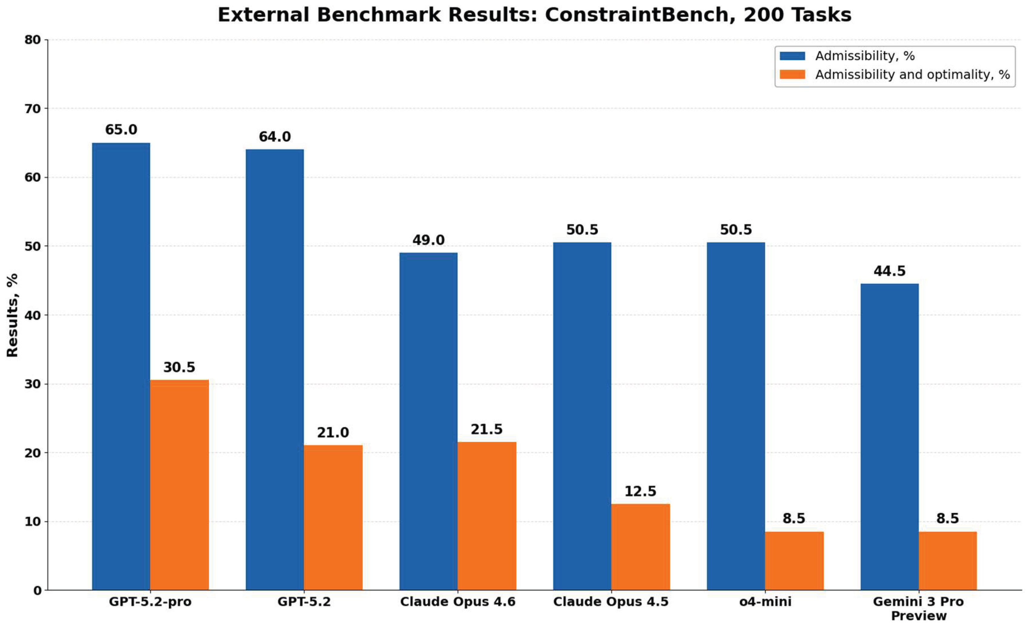
Published results from ConstraintBench [6] are examined here for external context. In that study, six state-of-the-art language models solved 200 problems across ten operations-research domains without access to a formal solver; for each answer, an independent verifier assessed constraint compliance and objective-function quality. These data were not included in the internal statistical tests and are presented solely as an external benchmark for the robustness of direct neural-network solutions to constrained problems. Table 15 reproduces the published per-model admissibility, objective quality, joint admissibility-and-optimality, and format/API error counts for all six models evaluated in that study.
A direct numerical ranking of HIM-D against the ConstraintBench models would be inappropriate, since the internal corpus uses synthetic problems with 1024 configurations while ConstraintBench spans ten different optimization types and remote commercial models. The qualitative conclusion is nonetheless consistent: without formal verification, even strong neural-network systems frequently produce solutions that violate one or more conditions, and high objective quality among feasible solutions does not compensate for the risk of an infeasible configuration.
ConstraintBench admissibility rates are substantially higher than those of the internal pure neural networks (44.5–65.0% versus 17.4–19.1%), yet the proportion of solutions that are both admissible and optimal remains low (8.5–30.5%), reinforcing the general conclusion regarding the gap between the plausibility of an answer and a guarantee of its admissibility.
Figure 4.
External benchmark results reported for six contemporary large language models on the ConstraintBench suite of 200 constrained-optimization problems, reproduced from [6] (values as listed in Table 15). Blue bars show the share of admissible (fully constraint-satisfying) solutions; orange bars show the share that is jointly admissible and optimal. Even the strongest model (GPT-5.2-pro) is admissible on only 65.0% of problems and jointly admissible-and-optimal on 30.5%, underscoring that admissibility, not objective quality, is the binding limitation of unaided LLM solvers on this task family.
Figure 4.
External benchmark results reported for six contemporary large language models on the ConstraintBench suite of 200 constrained-optimization problems, reproduced from [6] (values as listed in Table 15). Blue bars show the share of admissible (fully constraint-satisfying) solutions; orange bars show the share that is jointly admissible and optimal. Even the strongest model (GPT-5.2-pro) is admissible on only 65.0% of problems and jointly admissible-and-optimal on 30.5%, underscoring that admissibility, not objective quality, is the binding limitation of unaided LLM solvers on this task family.
6. Discussion
6.1. Main Conclusion
These results quantitatively support the central architectural thesis of the original work [1]: mandatory formal verification changes the guaranteed class of outcomes, not merely the average accuracy. This conclusion should, however, be stated at the architectural level rather than as a claim of universal superiority for deterministic AI. HIM-D was an exact reference by definition, whereas the two neural networks performed direct inference without a constraint-aware layer. A substantively important gap emerged in full admissibility: locally plausible choices frequently failed to form a consistent configuration. The procedural hybrid eliminated this risk because no unverified result was ever presented as final.
The HIM-D result is not a statistical surprise and should not be presented as evidence for a general scientific hypothesis; it establishes an achievable upper bound in a finite space where all constraints are known and exhaustive search is computationally cheap. The scientific value of the experiment lies in measuring the gap between an unverified candidate and a verified route, and in demonstrating that the ultimate reliability of the hybrid is determined by the control-transfer contract rather than by network quality alone. Scalability, incomplete requirements, rule errors, and more complex discrete structures remain open questions for future work.
6.2. Why Neural Networks Lost Admissibility
The pure neural-network models received all threshold and compatibility information but were trained using cross-entropy on individual group solutions. This loss function encourages matching the optimal class within each group but does not strictly prohibit globally incompatible combinations. The attention mechanism improved the result only moderately. The dominance of multiple simultaneous violations shows that errors are interrelated: the choice of one element simultaneously affects budget, risk, quality, and compatibility with several other elements. A robust solution therefore requires either training that directly incorporates formal constraints and verifier feedback, or the inclusion of an exact or approximate solver within the computational loop.
6.3. Practical Role of the Hybrid Architecture
The hybrid system eliminated all invalid outputs through a clear separation of responsibilities: the neural network neither validated its own decision nor modified the rules, and its only function was to generate a candidate. The verifier independently recomputed the constraints, and HIM-D received control only when verification failed. The guarantee of validity therefore derived not from any property of the network, but from the fact that no result was returned to the user before formal verification. The hybrid did not always reach the global optimum, since a valid neural-network candidate was accepted without re-optimization. In applications where the cost of error or of computation is particularly high, the rule can be tightened-for example, by running HIM-D for every instance, or by accepting a neural-network candidate only after a provable optimality-gap estimate.
The proportion of backup-search invocations was 80.88%, meaning the fast neural-network route was used for only 19.12% of tasks. This value coincides with the feasibility of the pure attention network, since the switching condition depended solely on the full feasibility of its argmax candidate. The compact network has thus, so far, only marginally reduced the computational load on the formal kernel. To improve the hybrid further, the network should be trained not only to reproduce the optimal configuration but also to predict the feasible region, the active constraints, a high-quality warm start, and a calibrated probability of constraint violation.
6.4. Implications for Education, Engineering, and Commerce
In educational systems, a neural network can interpret a problem statement, adapt an explanation, and select a difficulty level, but the mathematical correctness of the task and solution must be confirmed by symbolic or numerical verification. In engineering applications, safety, compatibility, and resource requirements must remain formalized, version-controlled rules; a neural network may propose and rank options but should not single-handedly resolve constraint conflicts. In a commercial configurator, a dialogue model reduces the user's cognitive load, while a deterministic core eliminates incompatible configurations, incorrect prices, and unrealistic promises. This pattern echoes the broader shift from purely predictive to prescriptive analytics, in which decision quality, not merely predictive accuracy, is the object of evaluation [27]. Table 16 translates these domain-level observations into a practical decision rule, matching five representative application contexts to the minimum evidentiary requirement each imposes, and the architecture recommended to meet it.
6.5. Comparison with the Targeted Literature
These results are consistent with the typology of machine learning for combinatorial optimization [4,5]. The feedforward networks in the present experiment solved the problem as a multi-output classification task and did not employ a formal algorithm within the loop; their low overall feasibility is therefore not inconsistent with studies in which ML strengthens the solver, differentiates through it, or projects the output onto the feasible set [21,22,23,24,25,26]. On the contrary, the comparison clarifies why such integrated methods are necessary for a stronger neural-network baseline.
The procedural hybrid is closer to solver-backed systems than to pure neural symbolism. Like OptiMUS, it separates the interpretive component from the formal solver [9], but in the present corpus the input is already machine-readable, so it is the quality of the final candidate, rather than the formulation step, that is tested. Unlike ConstraintBench [6], the formal module here does not merely evaluate the error after the fact-it corrects the route before the result is issued. This distinction explains the hybrid's 100% final admissibility despite the low admissibility of the network itself. The high proportion of backup-search invocations (80.88%) indicates that the current network only marginally reduces the workload of the formal core. Based on the literature reviewed, three further directions appear most promising: training the network to predict the feasible domain; using a differentiable or black-box solver within the loop; and using the network for a warm start and search reduction, without allowing it to return an unverified answer.
6.6. Theoretical Implications and Scientific Novelty
This study clarifies the role of hierarchical imitation models within modern AI architecture. Their advantage manifests not as a universal learning capability, but as a mechanism for explicitly representing the feasible domain, applying rules reproducibly, logging decisions, and enabling independent verification. The novelty of this work lies in operationalizing this principle within a single corpus and in separately measuring three levels: the quality of the direct candidate, the correctness of the verifier, and the behavior of the conditional fallback. This separation makes it possible to analyze the reliability of the hybrid without attributing a formal guarantee to the neural network itself.
7. Limitations of the Study
The first limitation concerns the synthetic nature of the corpus and the method used to define subject content. The twelve explicitly described scenarios make the composition of problems transparent, but they do not transform the corpus into real educational, engineering, or commercial data. Component names are semantic interpretations of variant indices; the actual numerical distributions were defined at the level of the three general parameterizations. The corpus does not reflect ambiguous textual requirements, incomplete catalogs, temporary availability, specification errors, regulatory documents, or expert disagreement. Before practical deployment, separate studies on real, anonymized problems with subject-matter expertise and predefined criteria for external validity are needed.
The second limitation concerns the moderate size of the configuration space. A complete search of 1024 options guaranteed the global optimum at low latency; increasing the number of groups or alternatives would require branch-and-bound, constraint programming, mixed-integer optimization, decomposition, or approximation methods. The full correctness achieved in the present experiment therefore does not demonstrate the scalability of exhaustive search.
The third limitation concerns the neural-network baseline models, which were intentionally compact and trained for a limited number of epochs on a CPU. Larger models, constraint-aware loss functions, differentiable optimization layers, and solver-feedback learning could substantially improve feasibility. However, external results from ConstraintBench show that even considerably more powerful language models do not eliminate the formal-robustness problem [6].
The fourth limitation is the indirect nature of the external comparison. The language-model metrics are drawn from another study and do not constitute a randomized comparison on a single corpus. A useful next step would be to run selected open-source and commercial models on the same 6,000 tasks, using the same inference scheme, token budget, and independent verifier.
The fifth limitation is the absence of user study. This work evaluates machine correctness and computational properties but does not measure trust, ease of interaction, or the system's influence on human decisions. Assessing the educational and commercial utility of the system would require a separate study with human participants, pre-approved by an ethics committee.
The sixth limitation concerns the design of the comparative baselines. The neural networks were trained with a single seed and were not compared with CP-SAT, MILP, LinSATNet, projection networks, or solver-in-the-loop training on the same corpus. Because the exhaustive HIM-D search simultaneously specifies both the exact solution and the reference boundary, this paper evaluates the architectural validation effect but does not establish superiority over modern exact and constraint-aware methods. For submission to a demanding Q1 journal, it would be advisable to add multiple independent training seeds, a CP-SAT or MILP baseline, a constraint-aware ablation, and a scaling analysis over the number of groups and variants.
The seventh limitation concerns the external validity of the synthetic generator. Guaranteed decidability and thresholding relative to a reference configuration can create regularities that are absent from real catalogs. A useful next step would include expertly labeled real or semi-synthetic configurations, inter-expert agreement checks, and separate validation of rule correctness. General principles for the verification and validation of simulation models require distinguishing among implementation correctness, conformity with the conceptual model, and applicability to the real system [29].
8. Conclusions
This study experimentally validates the architectural principle of separating probabilistic decision generation from independent formal verification, using configuration problems with hard constraints. Unlike the earlier conceptual work, which proposed HIM architecture at the methodological level, this article translates it into quantitatively verifiable experimental research. To this end, a reproducible computational corpus of 24,000 configuration problems was generated, a unified evaluation protocol was developed, research hypotheses were pre-specified, a system of quantitative metrics was defined, and deterministic, neural-network, and procedural-hybrid architectures were compared under identical testing conditions.
The results show that the primary advantage of a formal architectural component lies not in prediction quality but in its ability to guarantee satisfaction of the global constraints of a configuration task. Even modern neural-network models that achieve relatively high local accuracy in selecting individual components do not provide an acceptable probability of producing a globally feasible configuration. This effect becomes especially pronounced under controlled distribution shift, when the feasibility of direct neural-network solutions decreases sharply, whereas architectures incorporating independent formal verification maintain stable results.
The experiment confirms the effectiveness of a procedural hybrid approach in which a neural-network model is used exclusively for candidate generation, while the final solution is determined by independent validation and, when necessary, exact deterministic search. This approach achieves full correctness of the final result without sacrificing the advantages of statistical methods for generating initial solutions, and it supports the feasibility of functionally separating computational roles between the probabilistic and determined components of intelligent architecture.
The scientific novelty of this work lies not only in the numerical results obtained but also in the creation of a reproducible experimental methodology for evaluating configurational AI architectures. This is, to our knowledge, the first study to propose a unified protocol for the quantitative comparison of different architectural approaches, combining a reproducible task generator, fixed training and test sets, separate testing under ID and OOD distributions, a unified set of quantitative metrics, paired statistical analysis, reproducibility control, and an external comparison with published results for modern language models. This experimental design can serve as an independent basis for subsequent comparisons of new artificial-intelligence architecture designed to solve configurational and other problems with formal constraints.
The practical value of the study derives from the fact that the proposed experimental methodology is independent of the specific implementation of the neural-network model or the deterministic solver. It allows new architectures-differentiable optimization layers, solver-backed LLMs, agentic AI, and other neural-network systems-to be incorporated sequentially while a single, reproducible evaluation protocol is maintained, enabling accurate quantitative comparison across computing architectures without changing experimental conditions.
The results should nonetheless be interpreted in light of the study's limitations. All experiments were performed on a synthetic corpus of fixed structure with a finite search space of 1024 configurations, and the deterministic module was implemented via exhaustive search. The results therefore do not demonstrate the scalability of the proposed architecture to substantially more complex configuration spaces; rather, they demonstrate the influence of architectural principles on the reliability, reproducibility, and robustness of solutions within a fully controlled experimental environment.
Future research should expand the class of architectures studied, incorporate larger-scale deterministic solvers (CP-SAT, MILP, and other discrete-optimization methods), use real industrial configuration data, study integration with agent-based and language models, and develop a unified experimental setup for the comparative evaluation of verifiable AI architectures of various types.
Conflicts of Interest
The authors declare no conflict of interest.
Appendix A. Precise Implementation Parameters
Table A1 records every implementation detail needed to reproduce the neural-network models and the hybrid rule described in Section 4.3 and Section 4.4-architecture sizes, parameter counts, optimizer settings, the decoding and hybrid-switching rules, and the computing environment-so that the results in Section 5 can be regenerated exactly from the supplementary code.
Table A1.
Hyperparameters and implementation settings.
| Component | Value |
| Random seed (generation and training) |
20260711 |
| Number of tasks | 24,000, including 6000 test tasks |
| Configuration space | 5 groups × 4 variants = 1024 configurations |
| Residual MLP architecture | Input 435; hidden layer 384; residual block 384; dropout 0.08; output 5 × 4 |
| Residual MLP parameters | 471,572 |
| Residual MLP training | AdamW; lr 0.001; batch size 512; 5 epochs; weight decay 0.0001 |
| Attention network architecture | 5 tokens × 87 features; projection dimension 32; one attention block; FFN width 64; output 4 per token |
| Attention network parameters | 10,596 |
| Attention network training | AdamW; lr 0.0008; batch size 512; 3 epochs; weight decay 0.0001 |
| Neural-network decoding rule | argmax within each group |
| Hybrid rule – neural step | = argmax of the attention network, then independently checked against all hard constraints |
| Hybrid rule – fallback step | On any violation, exhaustively search the 1024 configurations and select the feasible option minimizing J(x) |
| Optimality criterion | Admissible and relative gap ≤ 0.1% |
| Computing environment | CPU; Python; NumPy; PyTorch 2.10.0+cpu |
Appendix B. Minimum Reproducibility Log Schema
Table B1 specifies the minimum schema for the per-instance log referenced in Section 2.4 and Section 4.7: each field's name, data type, and description are given so that the decision path, the verification outcome, and the objective-function values recorded for every task can be audited independently of the code that produced them.
Table B1.
Fields of the reproducibility log.
| Field | Type | Description |
| instance_id | string | Unique task identifier |
| domain | categorical | Education, engineering, or commerce |
| split | categorical | Training, validation, ID test, or OOD test |
| system_id | string | Algorithm or neural-network version |
| seed | integer | Random seed used for generation and the run |
| predicted_configuration | array | Five selected options |
| feasible | Boolean | Result of independent verification |
| violated_constraints | array | List of violated conditions |
| objective_value | number | Recomputed value of the objective function |
| optimal_objective | number | Reference (optimal) objective value |
| objective_gap | number | Relative gap, % |
| latency_ms | number | Execution time |
| model_hash | string | Checksum of the model version |
| scenario_code | string | Code for one of the 12 subject scenarios (E1–E4, I1–I4, or C1–C4) |
| scenario_name | string | Human-readable name of the configuration task |
| hybrid_route | categorical | neural_accept or him_fallback |
References
- Yavich, R.; Malev, S.; Volinsky, I.; Rotkin, V. Configurable Intelligent Design Based on Hierarchical Imitation Models. Appl. Sci. 2023, 13, 7602. [Google Scholar] [CrossRef]
- Mittal, S.; Frayman, F. Towards a Generic Model of Configuration Tasks. In Proceedings of the 11th International Joint Conference on Artificial Intelligence, Detroit, MI, USA, 20–25 August 1989; pp. 1395–1401. [Google Scholar] [CrossRef]
- Sabin, D.; Weigel, R. Product Configuration Frameworks-A Survey. IEEE Intell. Syst. Their Appl. 1998, 13, 42–49. [Google Scholar] [CrossRef]
- Bengio, Y.; Lodi, A.; Prouvost, A. Machine Learning for Combinatorial Optimization: A Methodological Tour d'Horizon. Eur. J. Oper. Res. 2021, 290, 405–421. [Google Scholar] [CrossRef]
- Cappart, Q.; Chételat, D.; Khalil, E.B.; Lodi, A.; Morris, C.; Veličković, P. Combinatorial Optimization and Reasoning with Graph Neural Networks. J. Mach. Learn. Res. 2023, 24, 1–61. [Google Scholar] [CrossRef]
- Tso, J.; Schmittou, P.; Huynh, Q.; Hutchins, J. ConstraintBench: Benchmarking LLM Constraint Reasoning on Direct Optimization. arXiv 2026, arXiv:2602.22465. [Google Scholar] [CrossRef]
- Chen, J.; Wei, Z.; Ren, Z.; Li, Z.; Zhang, J. LR²Bench: Evaluating Long-Chain Reflective Reasoning Capabilities of Large Language Models via Constraint Satisfaction Problems. Find. Assoc. Comput. Linguist. ACL 2025, 2025, 6006–6032. [Google Scholar] [CrossRef]
- Yang, Z.; Wang, Y.; Huang, Y.; Guo, Z.; Shi, W.; Han, X.; Feng, L.; Song, L.; Liang, X.; Tang, J. OptiBench Meets ReSocratic: Measure and Improve LLMs for Optimization Modeling. In Proceedings of the International Conference on Learning Representations (ICLR 2025), Singapore, 24–28 April 2025. [Google Scholar] [CrossRef]
- Ahmaditeshnizi, A.; Gao, W.; Udell, M. OptiMUS: Scalable Optimization Modeling with (MI)LP Solvers and Large Language Models. Proc. 41st Int. Conf. Mach. Learn. PMLR 2024, Volume 235, 577–596. [Google Scholar] [CrossRef]
- Rudin, C. Stop Explaining Black Box Machine Learning Models for High Stakes Decisions and Use Interpretable Models Instead. Nat. Mach. Intell. 2019, 1, 206–215. [Google Scholar] [CrossRef] [PubMed]
- Gorishniy, Y.; Rubachev, I.; Khrulkov, V.; Babenko, A. Revisiting Deep Learning Models for Tabular Data. Adv. Neural Inf. Process. Syst. 2021, 34, 18932–18943. [Google Scholar] [CrossRef]
- Huang, X.; Khetan, A.; Cvitkovic, M.; Karnin, Z. TabTransformer: Tabular Data Modeling Using Contextual Embeddings. arXiv 2020, arXiv:2012.06678. [Google Scholar] [CrossRef]
- Perron, L.; Didier, F.; Gay, S. The CP-SAT-LP Solver. Proc. 29th Int. Conf. Princ. Pract. Constraint Program. (CP 2023) LIPIcs 2023, Vol. 280, 3:1–3:2. [Google Scholar] [CrossRef]
- Sculley, D.; Holt, G.; Golovin, D.; Davydov, E.; Phillips, T.; Ebner, D.; Chaudhary, V.; Young, M.; Crespo, J.-F.; Dennison, D. Hidden Technical Debt in Machine Learning Systems. Adv. Neural Inf. Process. Syst. 2015, 28. [Google Scholar] [CrossRef]
- Mitchell, M.; Wu, S.; Zaldivar, A.; Barnes, P.; Vasserman, L.; Hutchinson, B.; Spitzer, E.; Raji, I.D.; Gebru, T. Model Cards for Model Reporting. In Proceedings of the Conference on Fairness, Accountability, and Transparency (FAT* 2019), 2019; pp. 220–229. [Google Scholar] [CrossRef]
- Efron, B.; Tibshirani, R. An Introduction to the Bootstrap; Chapman and Hall/CRC: New York, NY, USA, 1993. [Google Scholar] [CrossRef]
- Wilson, E.B. Probable Inference, the Law of Succession, and Statistical Inference. J. Am. Stat. Assoc. 1927, 22, 209–212. [Google Scholar] [CrossRef]
- Lakens, D. Equivalence Tests: A Practical Primer for t Tests, Correlations, and Meta-Analyses. Soc. Psychol. Personal. Sci. 2017, 8, 355–362. [Google Scholar] [CrossRef] [PubMed]
- Paszke, A.; Gross, S.; Massa, F.; Lerer, A.; Bradbury, J.; Chanan, G.; Killeen, T.; Lin, Z.; Gimelshein, N.; Antiga, L.; et al. PyTorch: An Imperative Style, High-Performance Deep Learning Library. Adv. Neural Inf. Process. Syst. 2019, 32. [Google Scholar] [CrossRef]
- Benjamini, Y.; Hochberg, Y. Controlling the False Discovery Rate: A Practical and Powerful Approach to Multiple Testing. J. R. Stat. Soc. Ser. B 1995, 57, 289–300. [Google Scholar] [CrossRef]
- Amos, B.; Kolter, J.Z. OptNet: Differentiable Optimization as a Layer in Neural Networks. Proc. 34th Int. Conf. Mach. Learn. PMLR 2017, Volume 70, 136–145. [Google Scholar] [CrossRef]
- Vlastelica, M.; Paulus, A.; Musil, V.; Martius, G.; Rolínek, M. Differentiation of Blackbox Combinatorial Solvers. In Proceedings of the International Conference on Learning Representations (ICLR 2020), 2020. [Google Scholar] [CrossRef]
- Paulus, A.; Rolínek, M.; Musil, V.; Amos, B.; Martius, G. CombOptNet: Fit the Right NP-Hard Problem by Learning Integer Programming Constraints. Proc. 38th Int. Conf. Mach. Learn. PMLR 2021, Volume 139, 8443–8453. [Google Scholar] [CrossRef]
- Liang, E.; Chen, M.; Low, S.H. Low Complexity Homeomorphic Projection to Ensure Neural-Network Solution Feasibility for Optimization over (Non-)Convex Set. Proc. 40th Int. Conf. Mach. Learn. PMLR 2023, Volume 202, 20623–20649. Available online: https://proceedings.mlr.press/v202/liang23a.html.
- Wang, R.; Zhang, Y.; Guo, Z.; Chen, T.; Yang, X.; Yan, J. LinSATNet: The Positive Linear Satisfiability Neural Networks. Proc. 40th Int. Conf. Mach. Learn. PMLR arXiv 2023, Volume 202, 36605–36625. [Google Scholar] [CrossRef]
- Min, Y.; Sonar, A.; Azizan, N. HardNet: Hard-Constrained Neural Networks with Universal Approximation Guarantees. arXiv 2024, arXiv:2410.10807. [Google Scholar] [CrossRef]
- Bertsimas, D.; Kallus, N. From Predictive to Prescriptive Analytics. Manag. Sci. 2020, 66, 1025–1044. [Google Scholar] [CrossRef]
- Pineau, J.; Vincent-Lamarre, P.; Sinha, K.; Larivière, V.; Beygelzimer, A.; d'Alché-Buc, F.; Fox, E.; Larochelle, H. Improving Reproducibility in Machine Learning Research: A Report from the NeurIPS 2019 Reproducibility Program. J. Mach. Learn. Res. 2021, 22, 1–20. Available online: https://www.jmlr.org/papers/volume22/20-303/20-303.pdf.
- Sargent, R.G. Verification and Validation of Simulation Models. J. Simul. 2013, 7, 12–24. [Google Scholar] [CrossRef]
Figure 1.
Deterministic and hybrid solution regimes. Panel A: the baseline HIM-D regime performs an exhaustive search over the 1024-configuration space and returns a result confirmed by a final verification step, V(u, x*). Panel B: the procedural hybrid regime in which the neural attention network Nθ proposes a candidate, an independent verifier evaluates V(u, ), and control passes to HIM-D for an exact backup search only when the candidate violates at least one hard constraint (V = 0); otherwise, the candidate is accepted directly. Both routes are logged with the selected path, any violations, the objective value J(x), and the applicable rule version.
Figure 1.
Deterministic and hybrid solution regimes. Panel A: the baseline HIM-D regime performs an exhaustive search over the 1024-configuration space and returns a result confirmed by a final verification step, V(u, x*). Panel B: the procedural hybrid regime in which the neural attention network Nθ proposes a candidate, an independent verifier evaluates V(u, ), and control passes to HIM-D for an exact backup search only when the candidate violates at least one hard constraint (V = 0); otherwise, the candidate is accepted directly. Both routes are logged with the selected path, any violations, the objective value J(x), and the applicable rule version.
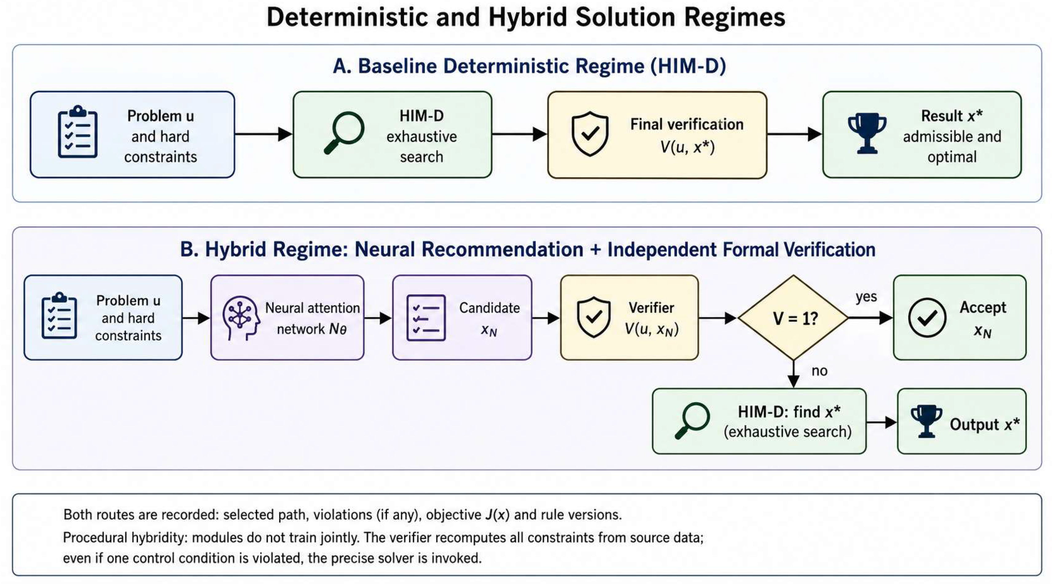
Figure 2.
Admissibility and joint admissibility-and-optimality of the four compared systems on the full test corpus (n = 6000), corresponding to the values in Table 9. Blue bars show the share of fully feasible configurations; orange bars show the share that is both feasible and within 0.1% of the optimal objective value. HIM-D and the hybrid system reach 100.0% on both metrics, while the Residual MLP and the group-attention network - evaluated without any formal verification layer - remain below 20% feasible and below 3% jointly feasible and optimal.
Figure 2.
Admissibility and joint admissibility-and-optimality of the four compared systems on the full test corpus (n = 6000), corresponding to the values in Table 9. Blue bars show the share of fully feasible configurations; orange bars show the share that is both feasible and within 0.1% of the optimal objective value. HIM-D and the hybrid system reach 100.0% on both metrics, while the Residual MLP and the group-attention network - evaluated without any formal verification layer - remain below 20% feasible and below 3% jointly feasible and optimal.
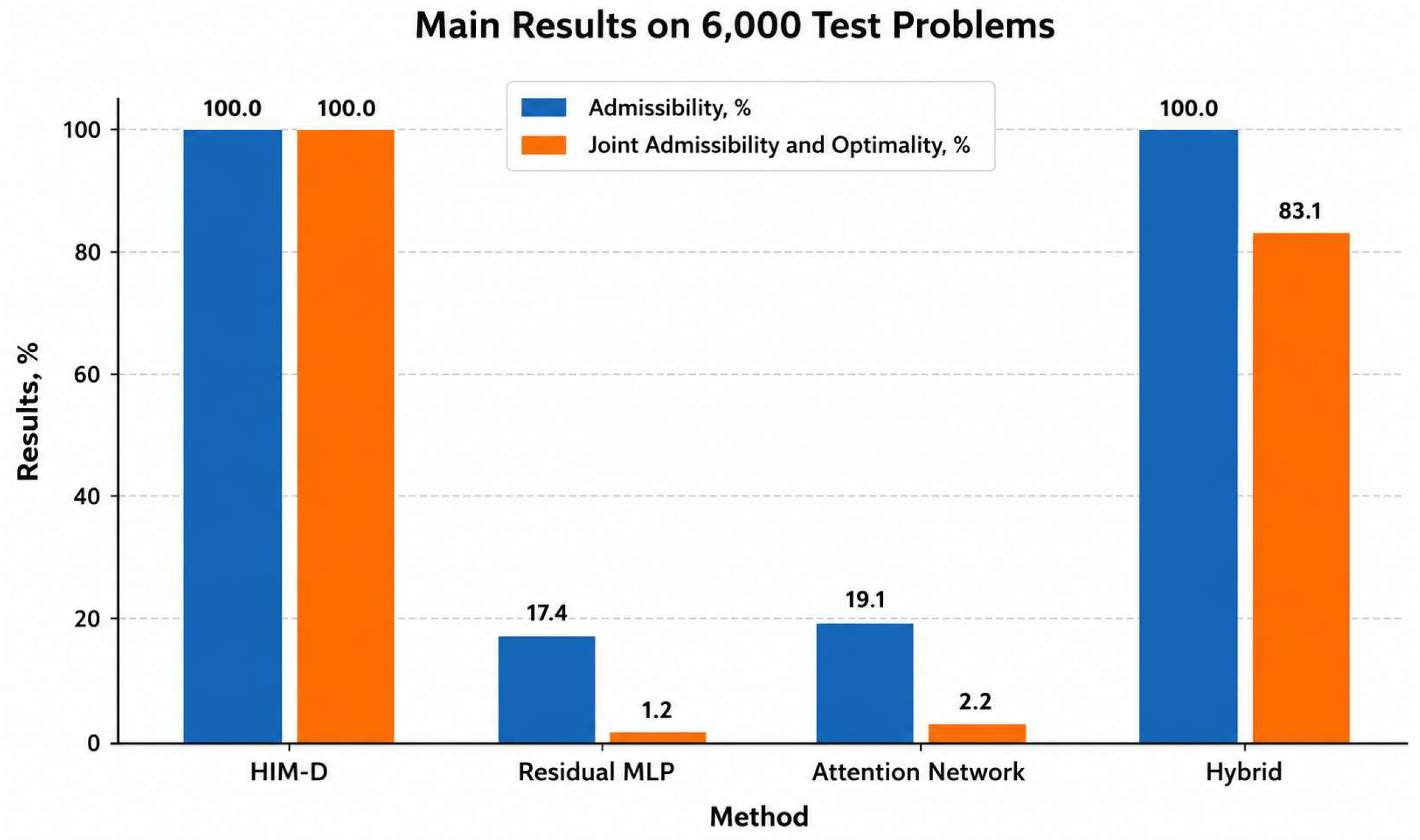
Figure 3.
Change in admissibility when moving from the in-distribution (ID) to the out-of-distribution (OOD) test subsample, for each of the four compared systems (Table 10). HIM-D and the hybrid system are unaffected (100.0% in both conditions), while the Residual MLP and the group-attention network lose more than three-quarters of their already-low admissibility under distribution shift, illustrating that direct neural-network inference without formal verification is not robust to OOD conditions.
Figure 3.
Change in admissibility when moving from the in-distribution (ID) to the out-of-distribution (OOD) test subsample, for each of the four compared systems (Table 10). HIM-D and the hybrid system are unaffected (100.0% in both conditions), while the Residual MLP and the group-attention network lose more than three-quarters of their already-low admissibility under distribution shift, illustrating that direct neural-network inference without formal verification is not robust to OOD conditions.
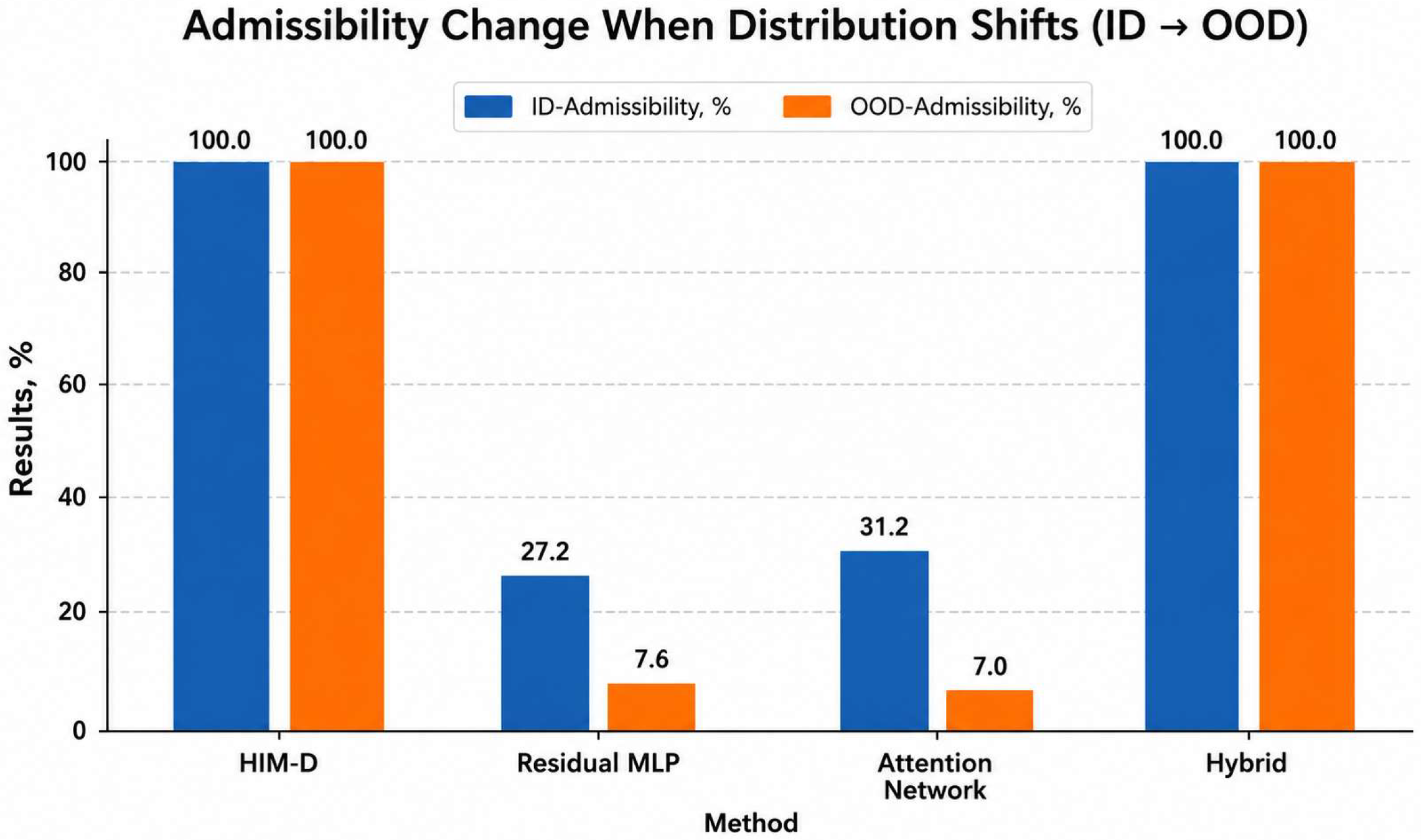
Table 1.
Transition from the conceptual provisions of the original architecture to the measured variables of the present study.
Table 1.
Transition from the conceptual provisions of the original architecture to the measured variables of the present study.
|
Position in the original architecture |
Operationalization in the present study | Primary indicator |
| Determinism | Explicit constraints and complete, verifiable search | Proportion of feasible and optimal solutions |
| Hierarchy of models | Levels of domain, solution group, variant, and constraint functional | Correctness across three subject domains |
| Reference library | Fixed library structure with versioned parameters | Reproducibility at a fixed granularity |
| Computational-complexity management | Finite space of 4⁵ = 1024 configurations | Latency per task |
| Dialogue with the user | Machine-readable requirements vector and explainable log | Traceability of selected configurations |
| Step-by-step validation | Training, validation, ID-test, and OOD-test splits | Separation of results across distributions |
Table 2.
Targeted synthesis of research directions and their relationship to the present work.
| Direction | Typical mechanism | Strong side | Limitation for the tasks considered | Role in the experiment |
| Configuration, CSP, CP/MILP [2,3,13] | Explicit variables, constraints, and exact search | Verifiable admissibility and optimality | Time grows with the expansion of the search space | HIM-D as the exact formal route |
| ML for solver enhancement [4,5] | Warm start, branch selection, search pruning | Preserves the formal core and can accelerate search | Requires integration with a specific solver | Justifies the role of the neural network as an auxiliary module |
| Direct neural-network solver [11,12] | Mapping the input directly to a configuration | Very low latency | No built-in guarantee of global compatibility | Residual MLP and group-attention network |
| Differentiable optimization [21,22,23,24,25,26] | Optimization layer, black-box solver, or projection | Constraints are involved in training or provided by design | Guarantee depends on the constraint class and the layer's implementation | Alternative route discussed as the next baseline |
| LLM with tools [8,9] | Text formalization, code generation, external solver | Flexible interface to optimization | Formulation errors and tool dependence | Context for separating interpretation from decision-making |
| Direct LLM solution [6,7] | Generating a ready-made solution without a solver | Universal natural-language interface | Admissibility remains narrow | External benchmark, not pooled with internal statistics |
| Procedural hybrid | Candidate generation, independent verification, conditional exact backup | Final admissibility across the full verification route | Savings depend on candidate quality; acceptability differs from optimality | Main verifiable architectural hypothesis of this study |
Table 3.
Composition of the corpus by split and domain (number of task instances).
| Corpus part | Education | Engineering | Commerce | Total | Purpose |
| Training | 5000 | 5000 | 5000 | 15,000 | Fitting neural-network weights |
| Validation | 1000 | 1000 | 1000 | 3000 | Quality control and model-state selection |
| ID test | 1000 | 1000 | 1000 | 3000 | In-distribution evaluation |
| OOD test | 1000 | 1000 | 1000 | 3000 | Evaluation under new ranges and dependencies |
| Total | 8000 | 8000 | 8000 | 24,000 | Full computational corpus |
Note: rows sum to the totals reported in Section 4.1 (15,000 training + 3,000 validation + 3,000 ID test + 3,000 OOD test = 24,000).
Table 4.
Compact description of the twelve tested configuration scenarios.
| Code | Task under test | Five joint decisions | Domain-specific meaning of the hard constraints |
| E1 | Personalized calculus lesson | Theory; explanation method; worked example; practice; assessment | Time/cost constraints, minimum pedagogical value, cognitive risk, consistency of lesson elements |
| E2 | Mathematics test set | Topic; difficulty; presentation; response type; feedback | Volume, coverage, acceptable complexity, format compatibility and verifiability |
| E3 | STEM laboratory exercise | Process; equipment; measurement; processing; report | Resource limit, data quality, procedural risk, equipment-and-method compatibility |
| E4 | Programming training module | Concept; language/environment; demonstration; practice; test | Time, minimum learning outcome, complexity/risk, compatibility of environment, tasks, and assessments |
| I1 | Sensor-node measurement unit | Sensor; converter; controller; communication; power supply | Price, accuracy, technical risk, electrical and interface compatibility |
| I2 | Industrial monitoring system | Measurement; data collection; computer; network; protective design | Budget, reliability, failure risk, protocol and operational compatibility |
| I3 | Thermal management system | Heat exchanger; pump/fan; sensor; controller; housing | Cost, thermal efficiency, risk, range and component-interface compatibility |
| I4 | Automated production cell | Actuator; controller; sensor; safety system; operator interface | Resources, performance, safety, control-and-protection compatibility |
| C1 | Computer equipment bundle | Processor; memory; storage; display; service | Price, performance, incompatibility risk, hardware-and-service consistency |
| C2 | Telecommunications plan | Data; voice; roaming; device; support | Monthly budget, utility, overpayment risk, tariff-and-technical compatibility |
| C3 | SaaS package | Tariff; users; storage; security; support | Cost, functional value, risk, licensing, security, and service alignment |
| C4 | Office equipment set | Printing; scanning; consumables; warranty; installation | Overall price, quality, operational risk, equipment-and-service compatibility |
Table 5.
Generation factors used to control task complexity and to form the OOD shift.
| Factor | ID level | OOD level | Role in the experiment |
| Number of groups | 5 | 5 | Size of the hierarchy |
| Options per group | 4 | 4 | 1024 configurations per task |
| Incompatibility density | 5–13% | 16–28% | Complexity of interaction constraints |
| Budget threshold | 102–114% of the reference cost | 100–103.5% of the reference cost | Resource stringency |
| Minimum quality | 87–99% of the reference quality | 96.5–100% of the reference quality | Quality stringency |
| Maximum risk | 102–114% of the reference risk | 100–103.5% of the reference risk | Safety stringency |
| Attribute ranges | Training ranges | Shifted cost and risk ranges | Out-of-distribution generalization |
Table 6.
Comparison of the systems evaluated in this study.
| System | Mechanism | Trainable parameters | Examination restrictions | Role |
| HIM-D | Explicit hierarchy; full search across 1024 configurations | 0 | Built-in, complete | Exact formal solver and reference upper bound |
| Residual MLP | Residual fully connected network; joint inference of 5 groups | 471,572 | None | Neural-network baseline model |
| Group-attention network | One token per group; single attention block; shared context | 10,596 | None | Compact structural neural network |
| Attention network + verifier + HIM-D | Nθ proposes ; V independently recomputes constraints; if V = 0, full enumeration via HIM-D | 10,596 trainable; formal modules untrained | Full, up to issuance of the result | Procedural hybrid with mandatory verification and conditional backup |
Table 8.
Task flow and adherence to the pre-registered protocol.
| Element | Planned | Actual | Deviation |
| Training tasks | 15,000 | 15,000 | None |
| Validation tasks | 3000 | 3000 | None |
| ID test | 3000 | 3000 | None |
| OOD test | 3000 | 3000 | None |
| Full test set | 6000 | 6000 | None |
| Stochastic repetitions | 5 × 500 tasks | 5 × 500 tasks | None |
| Random seed | 20260711 | 20260711 | None |
Table 10.
Admissibility and joint optimality within (ID) and outside (OOD) the training distribution.
Table 10.
Admissibility and joint optimality within (ID) and outside (OOD) the training distribution.
| System | ID admissibility, % | OOD admissibility, % | Decline, p.p. | ID joint optimality, % | OOD joint optimality, % |
| HIM-D | 100.00 | 100.00 | 0.00 | 100.00 | 100.00 |
| Residual MLP | 27.20 | 7.60 | 19.60 | 1.13 | 1.27 |
| Group-attention network | 31.20 | 7.03 | 24.17 | 2.93 | 1.47 |
| Attention network + deterministic verifier (hybrid) | 100.00 | 100.00 | 0.00 | 71.73 | 94.43 |
Table 12.
Structure of constraint violations among infeasible configurations.
| System | Incompatibility | Budget | Quality | Risk | Multiple violations | Total infeasible |
| Residual MLP | 1309 | 224 | 429 | 416 | 2578 | 4956 |
| Group-attention network | 1483 | 218 | 376 | 394 | 2382 | 4853 |
| Hybrid | 0 | 0 | 0 | 0 | 0 | 0 |
Note: totals equal 6000 minus the number of feasible configurations reported in Table 9 (6000 − 1044 = 4956 for the Residual MLP; 6000 − 1147 = 4853 for the group-attention network); the hybrid produced zero infeasible outputs by construction.
Table 14.
Summary of hypothesis tests.
| Hypothesis | Criterion | Observed result | Outcome |
| H1 | HIM-D advantage ≥ 5 p.p. | 82.60 p.p. vs. MLP; 80.88 p.p. vs. attention network; lower CI bounds > 79 p.p. | Confirmed |
| H2 | Smaller OOD decline for HIM-D | 0.00 p.p. vs. 19.60 and 24.17 p.p. | Confirmed |
| H3 | Higher repeatability | 100.0% vs. 0.0% across five stochastic runs | Confirmed |
| H4 | Hybrid not inferior to HIM-D within 1 p.p. | Difference of 0.00 p.p. | Confirmed |
| H5 | Hybrid improves joint optimality and keeps latency < 1 ms | 83.08% vs. 2.20%; 0.139 ms | Confirmed |
Table 15.
External benchmark: published ConstraintBench results on 200 problems [6].
Table 15.
External benchmark: published ConstraintBench results on 200 problems [6].
| Model | Admissibility, % | Objective quality among admissible, % | Joint admissibility and optimality, % | Format/API errors |
| GPT-5.2-pro | 65.0 | 95.2 | 30.5 | 1 |
| GPT-5.2 | 64.0 | 93.8 | 21.0 | 1 |
| Claude Opus 4.6 | 49.0 | 96.0 | 21.5 | 13 |
| Claude Opus 4.5 | 50.5 | 94.0 | 12.5 | 5 |
| o4-mini | 50.5 | 89.0 | 8.5 | 2 |
| Gemini 3 Pro Preview | 44.5 | 94.8 | 8.5 | 0 |
Table 16.
Recommended architecture by application risk level.
| Context | Minimum evidentiary requirement | Recommended architecture |
| Low-risk recommendation | Acceptable preference match, visible warning | Neural network with uncertainty reporting |
| Educational explanation | Verified mathematical correctness, solution log | Neural network plus a symbolic or deterministic verifier |
| Commercial equipment configurator | Full compatibility, accurate price, availability | Dialogue neural network plus a formal configurator |
| Engineering selection | 100% coverage of mandatory rules, version control | HIM-D or a formal solver with a neural-network interface |
| Critical system | Certified limits, independent verification, fail-safe behavior | Deterministic core; neural network only as an auxiliary module |
Disclaimer/Publisher’s Note: The statements, opinions and data contained in all publications are solely those of the individual author(s) and contributor(s) and not of MDPI and/or the editor(s). MDPI and/or the editor(s) disclaim responsibility for any injury to people or property resulting from any ideas, methods, instructions or products referred to in the content. |
© 2026 by the authors. Licensee MDPI, Basel, Switzerland. This article is an open access article distributed under the terms and conditions of the Creative Commons Attribution (CC BY) license (http://creativecommons.org/licenses/by/4.0/).
Copyright: This open access article is published under a Creative Commons CC BY 4.0 license, which permit the free download, distribution, and reuse, provided that the author and preprint are cited in any reuse.