

Submitted:
22 July 2026
Posted:
24 July 2026
You are already at the latest version
Abstract
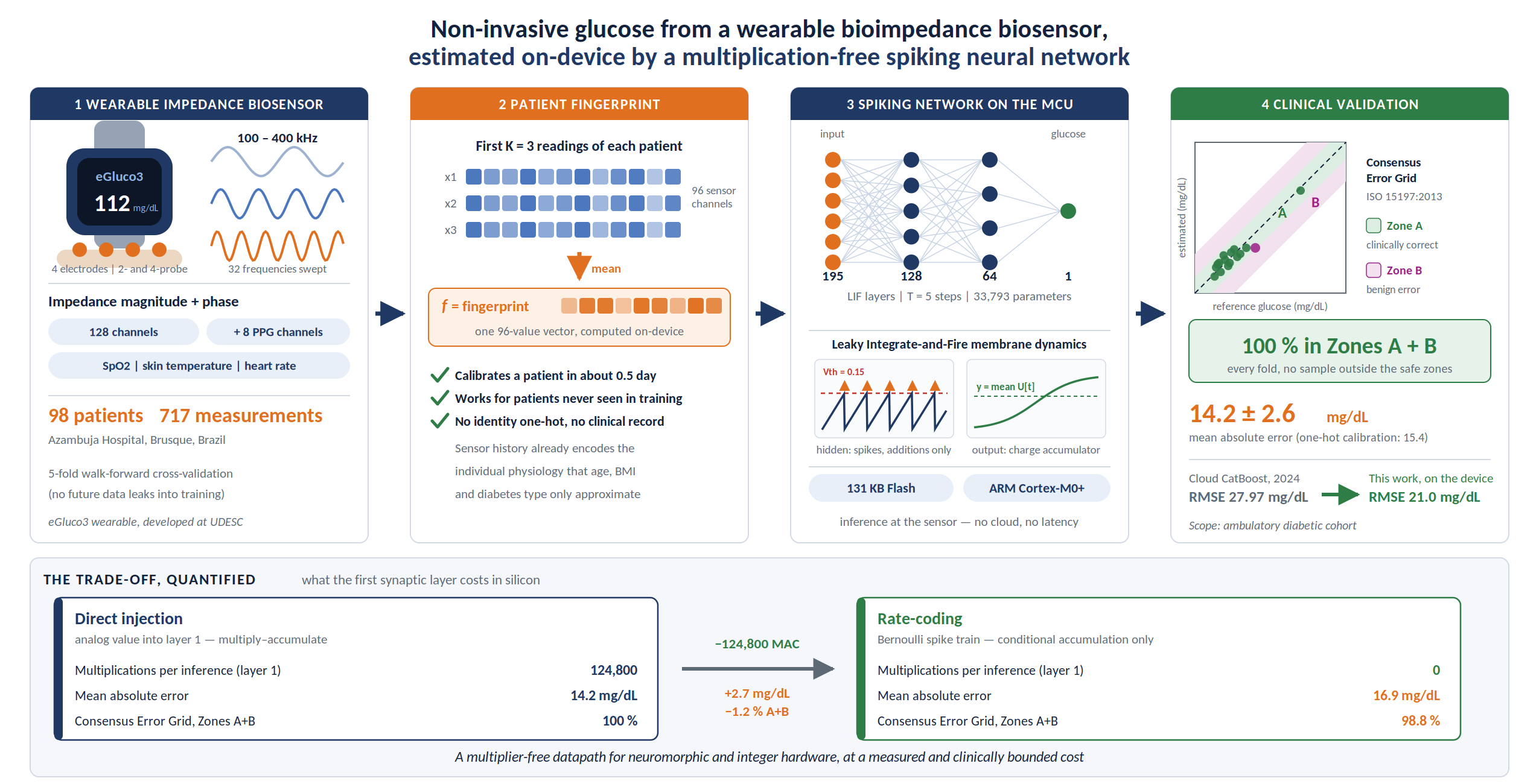
Wearable glucose monitoring demands ultra-low-power local processing, but conventional neural networks rely on energy-intensive multiply–accumulate (MAC) operations that limit battery life. This study shows that a Spiking Neural Network (SNN), built on a regression adapted Leaky Integrate-and-Fire (LIF) neuron, can estimate blood glucose from multi-frequency bioimpedance and auxiliary biosignals with clinical-grade accuracy at a fraction of the computational cost. Using data from 98 patients (717 measurements, eGluco3 device, Azambuja Hospital, Brusque, Brazil) evaluated by 5-fold walk-forward cross-validation under ISO 15197:2013, three main findings emerge. First, a new calibration method—the Patient Fingerprint, built from each patient’s first K sensor readings—outperforms conventional one-hot patient encoding (14.2 ± 2.6 mg/dL vs. 15.4 ± 3.3 mg/dL mean absolute error) while working for patients never seen during training, a capability one-hot encoding lacks entirely. Second, this fingerprint model reaches 100% of samples within Consensus Error Grid Zones A+B across all validation folds, meeting the clinical-safety threshold, and does so without requiring any demographic or clinical metadata—sensor history alone renders such records redundant. Third, replacing the analog input encoding with a multiplication-free rate-coding scheme removes all first-layer MAC operations at a cost of only 2.7 mg/dL additional error, defining a concrete, quantified accuracy–hardware trade-off for neuromorphic deployment. Together, these results demonstrate that SNNs offer a clinically validated, calibration-free, and computationally efficient path to continuous glucose estimation on embedded wearable devices.
Keywords:
spiking neural networks
; bioimpedance
; non-invasive glucose estimation
; edge AI
; neuromorphic regression
; embedded systems
; ISO 15197
; consensus error grid
; patient calibration
1. Introduction
The development of wearable technologies for continuous health monitoring requires the integration of biosensors with local computational intelligence. The central topic of this research is the non-invasive estimation of blood-glucose levels using multi-frequency bioimpedance spectroscopy. This multimodal approach yields high-dimensional physiological data, since the electrical properties of skin and cell membranes vary significantly across frequency sweeps (e.g., from 100 kHz to 400 kHz) [1,2]. However, deploying real-time predictive models directly on microcontroller-based wearable devices—a paradigm known as Edge AI—imposes severe constraints on hardware and energy consumption [3,4].
The fundamental problem addressed here is the high computational cost of conventional Artificial Neural Networks (ANNs) for this continuous-prediction task. ANNs rely on continuous floating-point data representations and require a massive number of energy-hungry multiply–accumulate (MAC) operations. For continuous monitors powered by small-capacity batteries, this traditional processing scheme leads to rapid energy depletion, precluding long-term autonomous operation [5,6].
To address this problem, we explore Spiking Neural Networks (SNNs) as a bio-inspired alternative for biosignal processing [2]. SNNs incorporate the notion of time into their operational model and communicate through discrete, sparse binary pulses (spikes). This event-driven nature replaces complex multiplications with simple additions, substantially reducing the energy needed for inference at the edge [3,7]. Moreover, although SNNs are widely used for classification, adapting their architecture for continuous regression is a promising challenge for the accurate estimation of biological parameters [8].
The overall objective of this work is to develop and evaluate a regression model based on Spiking Neural Networks capable of processing high-dynamic-range multi-frequency bioimpedance signals for non-invasive glucose estimation, with a primary focus on its computational feasibility for low-power embedded systems. To this end, the study first proposes the preprocessing and normalization of a clinical dataset—comprising bioimpedance measurements and contextual variables—formatted for temporal spike encoding. It then describes an SNN architecture based on the Leaky Integrate-and-Fire (LIF) neuron, specifically tuned for continuous regression. Training is performed off-line using Backpropagation Through Time (BPTT) together with Surrogate Gradient techniques. Finally, the research evaluates the model’s clinical accuracy using the error criteria defined by the international standard ISO 15197 [9] for glucose-monitoring systems, and maps its theoretical computational-cost profile to support a future embedded C/C++ implementation with dynamic calibration capabilities [10,11].
2. Background and Related Work
This section reviews the theoretical concepts underlying the project and presents recent work on neuromorphic networks for biosignal processing.
2.1. Concepts
Multi-frequency bioimpedance spectroscopy consists of the non-invasive measurement of the opposition of biological tissues to an alternating electrical current [12]. Dielectric properties vary dynamically across frequency sweeps (e.g., 100 kHz to 400 kHz), producing high-dimensional data that can be correlated with local metabolic parameters such as glucose.
Spiking Neural Networks (SNNs) are computational models that process information through discrete, sparse temporal events (spikes) [13]. They employ dynamical models such as the Leaky Integrate-and-Fire (LIF) neuron, emitting pulses only when the membrane potential crosses a threshold [14]. This replaces continuous multiplications with asynchronous additions, reducing computational cost.
Edge inference and regression. Edge AI processes data locally on the device, removing the dependence on servers. To adapt SNNs for continuous regression on edge hardware, the firing threshold of the output layer is suppressed, allowing the accumulated membrane potential to be read directly as an analog estimate.
2.2. Related Work
Focusing on computational feasibility for biomedical edge devices, Kim and Kim (2024) [1] and Choi (2024) [2] consolidate the algorithmic advantage of SNNs over conventional ANNs for biosignal analysis, showing that the sparse, event-driven nature of spiking networks converts complex MAC operations into simple conditional accumulations (additions). This substantial reduction in arithmetic complexity mitigates rapid battery drain, establishing SNNs as a promising approach for microcontroller implementations in healthcare.
Dealing specifically with non-invasive glucose prediction, Cruz Castañeda and Bertemes Filho (2024) [15] integrated multivariable biosensor data—bioimpedance, SpO2 and temperature—into an Edge-IoT model for smart cities. For remote processing, the authors established a broad baseline of twelve AI models, ranging from deep networks (1D-CNN, MLP) and classical approaches (SVR, KNN-R) to ensemble methods (Random Forest, AdaBoost). The best performance was obtained by a CatBoost regressor operating in the Cloud Learning Layer, reaching a test RMSE of 27.97 mg/dL. Although the result validates the clinical efficacy of bioimpedance, stress tests exposed the fragility of the centralized architecture: under a load of 50 concurrent users the system suffered a severe network bottleneck, with latency peaks of nearly 4 s (3737 ms) and an 11.46% request-failure rate. This delay shows that cloud dependence remains a critical operational barrier, reinforcing the need to move analytical inference entirely onto edge microcontrollers. Furthermore, the predecessor’s evaluation was limited to engineering metrics (MSE, RMSE, R2) and did not apply ISO 15197 as a clinical-validation criterion.
To overcome the limitations of edge architectures in analytical tasks, Lee et al. (2025) [8] investigated the feasibility of continuous prediction of local biological parameters. They proposed a model that extracts the spike rate from a neuromorphic network and applies Support Vector Regression (SVR) to continuously estimate heart rate from ECG signals. The results showed that this SNN–regression integration reaches accuracy comparable to conventional deep ANNs at a substantially lower computational cost, although it still depends on a secondary algorithm at the output stage.
Beyond theoretical feasibility, recent literature confirms the practical success of SNNs across biomedical engineering. Chu et al. (2023) [7] addressed accuracy loss in noisy ECG classification: using an SNN classifier enhanced with quantization-aware training, the system overcame raw-signal distortions and reached 98.24% accuracy in arrhythmia detection on wearable devices. Hens et al. (2025) [11] applied SNNs to complex biosignal classification for low-back-pain detection, introducing LAST (Learning Adaptive Spike Thresholds), a trainable encoder that adjusts firing thresholds dynamically, and obtaining over 80% accuracy. Zhao et al. (2023) [3] tackled continuous neural-signal monitoring on portable devices with an event-driven hybrid architecture, achieving accurate classification with extreme energy efficiency (0.99–4.38 J per class). Sava et al. (2023) [16] addressed SNN instability when processing high-dynamic-range medical data through recurrent and feed-forward inhibition that compress and stabilize physiological data at the network input. Reddy et al. (2024) [17] confronted the non-differentiability of spikes by combining BPTT with surrogate gradients, reaching about 86% accuracy with a very low-complexity architecture. Finally, Martis et al. (2025) [5] developed SYNtzulA, a custom SNN accelerator for near-sensor processing with a consumption of only 36.5 pJ per synaptic operation.
3. Materials and Methods
This work proposes a fully spike-based continuous glycemia-estimation architecture designed for autonomous execution on ultra-low-power embedded devices. Figure 1 presents an overview of the proposed system, from multimodal biosignal acquisition to clinical auditing under ISO 15197.
The methodology is structured as a motivated progression of design decisions, in which each stage starts from a limitation identified in the previous one. First, we establish the dataset, the validation protocol and the end-to-end LIF regression topology—exploring alternatives (discrete classification, hybrid SNN+SVR extraction) to justify the architectural choice. We then compare two input-encoding strategies—Direct Injection (MAC) and Rate-Coding (AC)—quantifying the trade-off between clinical accuracy and energy savings. The next stage investigates whether patient clinical-profile data (diabetes type, BMI, sex) improve individual accuracy, revealing that such metadata partially compensate for the absence of individualized physiological calibration. This finding motivated the core mechanism of the solution: the Patient Fingerprint, a calibration vector computed from the patient’s first K measurements that replaces one-hot encoding and, by not depending on identities seen in training, in principle enables the calibration of unseen patients. Finally, we evaluate the portability of the trained model to a distinct clinical cohort (ICU2025), delimiting the scope of the solution.
3.1. Dataset and Preprocessing
Cohort and acquisition. The study used multisensor monitoring data collected in a controlled clinical environment from two distinct campaigns: ambulatory patients diagnosed with diabetes (2024 campaign) and patients admitted to an intensive-care unit (2025 campaign), with capillary-glucose reference determined by a glucometer. After integrity validation and physiological filtering (steps 1–2 of the pipeline described below), the consolidated base comprises 98 patients and 717 multisensor measurements, concentrated in 2024 (67 patients, 575 measurements) and 2025 (31 patients, 138 measurements). From this base, the analysis cohorts summarized in Table 1 are derived, combining a temporal filter (ambulatory 2024 vs. ICU 2025) with a clinical-profile integrity criterion. The final model is trained and evaluated on the curated ambulatory cohort (sano2024); the ICU cohort serves only as the target domain of the transfer study. Each acquisition simultaneously records five biosignal modalities: (i) multi-frequency bioimpedance—magnitude (m) and phase (f) measured at 32 distinct frequencies in 2-probe and 4-probe configurations, totaling raw channels; (ii) photoplethysmography (PPG)—minimum and maximum amplitude per acquisition window at 4 wavelengths, yielding 8 optical channels; (iii) pulse oximetry (SpO2), 1 channel; (iv) skin temperature, 1 channel; and (v) heart and pulse rate, 1 channel.
Patient clinical profile. In addition to the sensor measurements, the database stores a per-patient clinical profile linked by a unique identifier. The available fields are date of birth (converted to age in years), height and weight (from which the body mass index, BMI, is derived), sex (; ), and diabetes type in clinical ordinal encoding (; ; ; ). The integrity criterion required height between 1.40 and 2.20 m, weight between 30 and 300 kg and age between 10 and 100 years. Of the 98 patients, 58 hold a real, valid clinical profile; the remaining 40 lacked a valid record. For the experiments based only on sensors and identity (one-hot), these 40 patients were retained—their clinical fields filled by the median and signaled by a flag—since such models do not consume clinical features. Conversely, any analysis that actually uses clinical features (enrichment and importance) was restricted to the subset of 58 patients with a real profile, avoiding contamination by imputed values.
Sanitization pipeline. Preprocessing followed a four-step sequence: (1) integrity validation—discarding records flagged as invalid by the device firmware (contact failure or motion artifact); (2) physiological filtering—retaining only records with reference glycemia in mg/dL (717 measurements from 98 patients after this step); (3) cohort filtering—selecting the sano2024 cohort, i.e., patients with at least 80% of measurements in 2024, restricting the study to contemporary, homogeneous data; and (4) zero-variance filtering—removing channels with null variance, leaving 96 active features for the model.
Analysis cohorts. From the sanitized base, the analysis cohorts of Table 1 are derived by combining the temporal split with the clinical-profile integrity requirement. The curated ambulatory cohort sano2024 (29 patients with an integral profile and ≥80% of measurements in 2024) supports the champion model, the importance analysis and the transfer source. The broad 2024 cohort (66 patients, no profile requirement) is used only in the scalability test of the sensor-only model, and the ICU2025 cohort (29 patients admitted in 2025) is the transfer target. The preliminary architecture explorations (classification, SNN+SVR and the input-encoding study) were conducted on the full 98-patient base—which mixes both campaigns and relies on profile imputation for the 40 patients without a valid record—and are therefore reported only as a preliminary baseline.
Temporal abstraction. Unlike conventional ANNs that map static matrices, SNNs operate in the time domain. To represent this biological dynamic, the analog signal was abstracted into sequential sliding windows. Ablation analyses (window sizes , and ) revealed the diminishing returns of temporal memory for this biosignal: overly wide windows introduced statistical noise and diluted the instantaneous glucose correlation, and at the requirement of continuous temporal sequences exhausted the viable windows per patient, precluding training. Therefore, the optimal abstraction window was set at discrete steps.
3.2. Validation Protocol: Walk-Forward Cross-Validation
To assess the temporal robustness of the models and prevent any leakage of future data into training, we adopted a 5-fold walk-forward cross-validation protocol. In each fold k, the training set spans and validation spans of each patient’s time series, with . Crucially, all patients appear in both sets of every fold, ensuring that the calibration one-hot is useful at inference. Fold 5 (the 80%/20% split) is reported as the principal result; the remaining folds provide robustness estimates (mean ± SD). The walk-forward scheme is illustrated in Figure 2.
3.3. Predictive Topologies Explored
Before consolidating the final end-to-end regression topology, two alternative approaches to the non-linear mapping of bioimpedance were investigated. Classification into discrete values: discretizing the glycemic spectrum into 10 and 25 mg/dL bins led to rapid overfitting, owing to the loss of the ordinal relation imposed by the CrossEntropy loss and the sample scarcity of boundary classes. Hybrid SNN+SVR architecture: using the SNN as a temporal feature extractor as proposed by Lee et al. [8], delegating the final prediction to an RBF-kernel SVR (, , ), proved suboptimal, since the hidden-layer firing rates—interpreted in isolation from their accumulated integrative potential—lost the representational richness needed to distinguish abrupt variations.
3.4. The Neuron Model for Continuous Regression
The fundamental element of the proposed architecture is the Leaky Integrate-and-Fire (LIF) neuron. The temporal dynamics of the membrane potential are governed by the decay equation:
where (fixed at 0.80) is the leak factor, is the synaptic weight, is the event presence (continuous current or binary spike) at the input synapse, and the term implements the subtractive reset after firing (). In the hidden layers the threshold is fixed at . In the output layer the firing mechanism is disabled (, hence for all t) and the leak is removed (, no leak), turning the neuron into a continuous charge accumulator; the temporal mean of its potential over the T steps directly represents the estimated glucose concentration. Figure 3 illustrates the membrane-potential behavior in both configurations.
3.5. Input-Encoding Topologies
To assess the trade-off between clinical predictive accuracy and energy savings on edge operations, two main data-injection schemes were developed. Direct Injection (temporal spike): the normalized analog signal is continuously converted into current and processed step by step. This preserves the full signal resolution and maximizes accuracy, but requires multiply–accumulate (MAC) operations in the first synaptic layer. Sparse encoding (Rate-Coding): the analog value is replaced by the spike-emission probability through a Bernoulli distribution, turning the first hidden layer into a purely additive (AC) operation matrix—the ideal solution for energy-limited architectures. In the baseline comparison (, no fingerprint), the stochastic evaluation was stabilized by averaging 30 Monte Carlo passes per sample. In the fingerprint variant (Section 3.7), the Straight-Through Estimator (STE) [18] was adopted: the gradient backpropagates through the Bernoulli operation as if the identity were applied (), removing the need for multiple samples during training. To compensate for the limited six-level resolution at , the number of rate-coding steps was decoupled from the temporal window: each window step was subdivided into microticks, with evaluated by ablation.
Both topologies were first evaluated with patient identification via one-hot encoding, without explicit clinical data. The next investigation examines whether incorporating clinical-profile metadata reduces residual mean bias and improves individual accuracy.
3.6. Enrichment with the Patient Clinical Profile
Motivated by the hypothesis that anthropometric and clinical factors influence the bioimpedance–glycemia correlation, we investigated a complementary model that concatenates to the sensor vector the five clinical-profile features of Section 3.1: age, BMI, sex, diabetes type and the has-profile flag. Data was collected from 98 patients from Azambuja Hospital in Brusque (Brazil) using the eGluco3 device, which was developed by the research group at Santa Catarina State University. This experiment, like the input-encoding comparison (Direct Injection vs. Rate-Coding), operates on the 98-patient cohort with one-hot identification. The strategy expands the input vector from to dimensions and adds 640 trainable parameters. The importance of each feature was quantified by architecture-agnostic Permutation Feature Importance: each feature is shuffled individually in the validation set and the MAE degradation is measured against the baseline, with 10 repetitions per feature for statistical stability. Although the clinical profile improves accuracy, one-hot encoding remains a critical operational restriction: the model only recognizes patients present in the training set, precluding deployment on commercial devices with new users.
3.7. Patient Fingerprint Calibration
The clinical-profile and one-hot model assumes that the device recognizes the user—a critical limitation for embedded deployment, since new patients require retraining. To overcome this, we investigated a dynamic calibration mechanism called the Patient Fingerprint: a vector computed as the arithmetic mean of the patient’s first K sensor vectors in the training window,
where denotes the 96 bioimpedance channels of the j-th chronologically ordered measurement. The vector is concatenated to every temporal step of the sliding window, expanding the input from to dimensions. Unlike one-hot, the fingerprint does not require the patient to be present in training—only K initial measurements are needed to personalize it.
Fingerprint evaluation—which consolidates the proposed final solution—adopts a stricter temporal filter than the previous experiments, requiring from each patient a continuous series long enough to compute the calibration vector under the walk-forward protocol (≥80% of measurements in 2024). This reduces the cohort to 29 patients (336 measurements) with dense temporal history. For a fair comparison, the reference one-hot model is retrained on this same 29-patient cohort, not on the 98-patient cohort used in the input-encoding study. Under this stricter filter, the has-profile flag becomes constant (zero variance, since all 29 patients hold a valid profile) and is dropped, while sex is evaluated and excluded for exhibiting negative permutation importance on this subset. Three active clinical features therefore remain—age, BMI and diabetes type—so the base windows hold channels. In this protocol, walk-forward quantifies temporal robustness on known patients (present in both training and validation of each fold), whereas generalization to unseen individuals is assessed separately in the cross-cohort transfer (Section 3.8). The effect of K was studied by ablation () in two variants: (a) windows holding the 99 base channels () and (b) windows restricted to the 96 sensor channels (), removing the dependence on clinical records and simulating a purely sensor-based device. A complementary temporal analysis quantified the mean interval between the first and K-th measurement per patient, assessing the calibration latency in a realistic clinical scenario.
3.8. Cross-Cohort Transfer Evaluation
To assess generalization to distinct clinical environments, a cross-cohort transfer study was conducted. The sano2024 set (ambulatory diabetic patients) was used as the source domain; the ICU2025 set, with patients admitted to an intensive care unit in 2025, as the target domain. The experiment adopted two approaches: (i) training the fingerprint model directly on the ICU cohort with the same walk-forward protocol (scarce data—10 to 23 training windows per fold—required a minimum threshold of windows and an adaptive batch size); and (ii) zero-shot transfer—full training on sano2024 without a train/validation split (220 windows), followed by direct evaluation on the ICU patients, aligning the feature space to that of sano2024 and reusing the glucose normalization scaler trained on sano2024 ( mg/dL).
3.9. Training and Implementation
The network is structured as densely connected layers with topology —the base configuration with one-hot patient identification; the clinical-profile and Patient Fingerprint variants adjust only the input-layer dimension—interleaved with Layer Normalization (LayerNorm) blocks to stabilize the internal membrane-integration dynamics. Training relied on Backpropagation Through Time (BPTT). Since the binary activation has no continuous derivative, the Surrogate Gradient method was applied as a fast-sigmoid approximation (slope ). The Adam optimizer was combined with the Smooth L1 (Huber) loss, which proved superior to the conventional mean squared error by damping the sparse variances inherent to sensor biology. A plateau-based learning-rate scheduler (ReduceLROnPlateau) with patience of 25 epochs and early stopping with patience of 60 epochs were used. Algorithm 1 formalizes the signal-propagation decisions of the proposed neuromorphic system.
| Algorithm 1: Regression processing in the proposed SNN |
|
3.10. Clinical Validation Criteria: ISO 15197:2013
Clinical conformity was assessed under two complementary criteria of ISO 15197 [9]. Criterion A (Section 6.3.3): at least 95% of results must meet a two-phase target: (i) for concentrations below 100 mg/dL, the absolute error must not exceed ±15 mg/dL; (ii) for concentrations ≥ 100 mg/dL, the percentage relative error must lie within ±15%. The Mean Absolute Relative Difference (MARD) is computed sample by sample:
Criterion B—Consensus Error Grid (CEG, Annex C): evaluates the clinical impact of errors by risk zones. The standard requires that at least 99% of samples remain in Zones A+B.
3.11. Computational-Cost Quantification
The operational cost per inference was quantified for the architecture with steps, distinguishing MAC (multiply–accumulate) from AC (conditional-accumulation) operations. For Direct Injection, the first layer always executes MACs, since the input is continuous; layers 2 and 3 execute ACs proportional to the measured firing rate. For Rate-Coding, the first layer executes only ACs (binary Bernoulli input). The hidden-layer firing rate was measured empirically by a forward pass over the fold-5 validation set, accumulating each layer’s spike tensors to obtain the mean fraction of neurons firing per time step.
3.12. Embedded Export and Portability
Since the premise of this work is autonomous edge inference, the off-line-optimized neuromorphic model was ported from PyTorch to C/C++. A bare-metal implementation was chosen, decoupled from high-level commercial inference frameworks, to maximize computational efficiency and ensure hardware agnosticism. A transversal extraction routine reads the trained-model parameter dictionary (a .pth file), isolates the synaptic weight matrices and bias vectors of each (Linear and LayerNorm) layer, flattens them into single-precision (float) one-dimensional arrays, and automatically transcribes them into a unified header (.h) file. A key architectural decision was the deterministic allocation of all extracted parameters directly in non-volatile memory (Flash/ROM), preserving the scarce SRAM exclusively for the dynamic update of the membrane potentials and the multimodal input buffers.
4. Results and Discussions
Except for the preliminary classification and SVR explorations—conducted on the broad cohort of the initial design and cited only to contextualize the architectural choice—the results in this section refer to the 29-patient cohort with a real clinical profile, evaluated by 5-fold walk-forward cross-validation; fold 5 (80%/20%) is the principal result and the mean ± SD of the five folds is the robustness measure. The evaluation unit is the prediction window (a sequence of consecutive measurements) rather than the patient: each validation set gathers the windows contained in the final 20% of each patient’s series, so the principal fold sums ≈17 windows, fewer than the cohort’s patients (short series yield few or no validation windows). The cohort used is indicated per experiment: analyses that depend on clinical features are restricted to patients with a valid profile, whereas sensor-only analyses can exploit the broad cohort. Clinical conformity follows Criteria A and B of ISO 15197:2013.
4.1. Overview of the Approaches
Table 2 consolidates the performance of the patient-calibration strategies on the 29-patient cohort, from no calibration to the final fingerprint mechanism. Beforehand, two alternative formulations explored on the broad cohort were discarded for structural reasons. Classification into discrete bins (25 and 10 mg/dL) reached only 58% and 46% accuracy (MAE of 28.1 and 29.6 mg/dL): discretization discards the ordinal relation between bins—CrossEntropy treats adjacent classes as independent—and the sample-scarce extreme bins drive the model to collapse onto two or three central bins near the physiological mean. The hybrid SNN+SVR architecture, delegating prediction to an SVR fed by hidden-layer firing rates, regressed to a MAE of 38.8 mg/dL: isolated from the accumulated membrane potential, firing rates lose the representational richness needed to distinguish abrupt glycemic variations. In both cases, end-to-end LIF regression proved superior, justifying the architectural choice.
Individual calibration is decisive: without it, the model is clinically unviable (MAE mg/dL). One-hot encoding learns a per-patient identity vector (15.4 mg/dL) but requires the patient to be in the training set—unviable for new users. The Patient Fingerprint surpasses one-hot (14.2 mg/dL) without that restriction, deriving calibration from only K initial measurements, and constitutes the final solution. Its rate-coding variant trades accuracy for energy efficiency, as detailed below.
4.2. Final Solution: Accuracy, Energy and Embedded Feasibility
The proposed solution materializes in two embeddable fingerprint variants, identical in architecture (, 33,793 parameters) and differing only in the first-layer encoding (Table 3). Direct Injection () preserves the analog signal resolution and delivers the lowest error ( mg/dL MAE; mg/dL RMSE in the walk-forward 5-fold CV, mg/dL in the principal fold), the highest temporal stability and 100% ISO B, at the cost of keeping MAC operations at the input. Rate-Coding () replaces that layer with purely additive (AC) operations via Bernoulli binarization—an ideal target for ultra-low-power neuromorphic hardware—at the cost of mg/dL MAE and a slight drop in Criterion B (98.8%).
Regarding cost per inference, Direct Injection executes MAC operations in the first layer alone. Rate-Coding eliminates them entirely, rendering the datapath multiplier-free—a prerequisite for the most efficient neuromorphic accelerators. The high microtick count of the winning configuration (, ten per measurement) is not arbitrary: since each normalized feature is encoded by its firing probability, few steps per measurement would offer very few discrete rate levels—only six at —insufficient to represent the dynamic range of bioimpedance; subdividing each measurement into ten microticks restores enough rate resolution to match direct injection. The counterpart is that processing 50 microticks (against 5 steps) multiplies the additive (AC) operations of the hidden layers by an order of magnitude, so the total operation count rises rather than falls. Whether trading multiplications for more additions yields a net energy gain depends on the target hardware—favorable on neuromorphic/integer hardware, where addition is the native, cheap operation, and marginal where the MAC–AC cost gap is small. The exact additive-operation count and energy balance depend on the firing rates measured in this 50-microtick regime and on the platform, and are quantified in the embedded implementation (future work). In both cases, the model occupies ≈131 KB of non-volatile memory (Flash/ROM), compatible with ARM Cortex-M0+ class microcontrollers.
4.3. Factors of Influence
Temporal window. The -step window proved the stability optimum: widening it to degraded the MAE to 62.2 mg/dL, and exhausted the continuous temporal windows available per patient, precluding training.
Calibration latency. The mean interval between the first and K-th measurement grows with K: ≈0.5 days for (compatible with calibration at the first consultation) and ≈4.7 days for , whose coverage drops to only 10 of the 29 patients—explaining the fingerprint degradation at high K.
Clinical features are context-dependent. The usefulness of demographic metadata is entirely conditioned on the context available to the model (Table 4). Without history (pointwise model, ), they become the most informative features—sex leads (ΔMAE mg/dL), followed by age () and diabetes type ()—yet the pointwise model remains clinically inadequate (MAE mg/dL; ISO B ). With temporal history, the clinical contribution collapses: diabetes type drops to mg/dL, age becomes noise () and sex flips sign ( mg/dL), behaving as a spurious shortcut in a small set—the reason for its exclusion from the deployed model. Consistently, the purely sensor-based fingerprint (no clinical data, ) matches the champion ( mg/dL), confirming that sensor history renders the clinical record dispensable.
Patient identity dominates. In the temporal model, permutation importance is led by individual identity (Table 5): the two most informative one-hot features ( and mg/dL) outweigh any single biomarker, motivating the per-patient calibration mechanism.
Cross-cohort generalization. Transfer to the intensive-care cohort (ICU2025, Table 6) delimits the application scope: zero-shot transfer collapses (MAE mg/dL; ISO B ), and even direct training on the ICU cohort remains clinically insufficient (48.2 mg/dL), owing to data scarcity (10–23 windows per fold). The model is therefore specific to the ambulatory diabetic population on which it was trained.
Scalability without clinical data. By dispensing with the clinical record, the sensor-only fingerprint allows relaxing the integral-profile requirement and including all 2024 patients—expanding the cohort from 29 to 66 patients (573 measurements). On this broad cohort, direct injection keeps clinical conformity (ISO B ≈ 99%) and, in the training-densest fold, recovers the curated-cohort accuracy (MAE mg/dL); robustness, however, degrades, with a mean MAE of mg/dL—and the noisier rate-coding degrades further. This drop reflects the greater heterogeneity of the cohort and, possibly, the lower reliability of records from patients without a clinical profile, whose missing profile may correlate with less-curated acquisitions. The experiment shows that the method scales without any clinical metadata but benefits from a dense, curated cohort to reach its best accuracy.
The preceding results support the following discussion of the clinical scope, the hardware trade-off and the generalization limits of the solution.
4.4. Clinical Positioning and Comparison with the State of the Art
Clinically, the champion model attains a MAE of 14.2 mg/dL with 100% of samples in Zones A+B (Criterion B) across all folds, surpassing one-hot (15.4 mg/dL) without requiring the patient in training. Conformity to Criterion A, however, remains below the 95% normative threshold, precluding formal certification—a limitation attributed to the small validation set and the sparse coverage of extreme ranges (detailed in the Limitations section). The largest errors concentrate in glycemic transitions: patients whose profile during training differs from that observed at validation, which the model cannot anticipate without recalibration—motivating online recalibration as future work.
Compared with the predecessor work of Cruz Castañeda and Bertemes Filho [15], whose best regressor (cloud CatBoost) reports RMSE mg/dL and R2 = 0.31, the local SNN attains competitive performance, with an RMSE of mg/dL in the walk-forward mean ( mg/dL in the principal fold), even though evaluated over the full glycemic range [70–600], wider and more challenging than the predecessor’s narrow test distribution. We note that R2 in isolation is sensitive to the dispersion of each test set—so RMSE and the deployment characteristics constitute the more robust comparison. Beyond accuracy, the SNN removes cloud dependence—whose latencies of up to 3737 ms and 11.46% failure rate under load are incompatible with critical continuous monitoring—and adds the normative ISO 15197 validation absent in the predecessor. The difference is also one of deployment: whereas CatBoost operates in the cloud, the SNN model occupies only ≈131 KB of Flash/ROM—compatible with ARM Cortex-M0+ class microcontrollers (≈256 KB)—enabling near-sensor inference. Table 7 summarizes the comparison.
4.5. The Hardware Trade-Off
The central technical contribution is the mapping of the trade-off between accuracy and hardware architecture. Rate-Coding eliminates the 124,800 first-layer multiplications, rendering the datapath entirely multiplier-free—in the direction of neuromorphic accelerators such as SYNtzulA [5]—at the cost of mg/dL MAE and an ISO B drop from 100% to 98.8%. Notably, with , this elimination does not reduce the total operation count: the hidden layers, processed over 50 microticks instead of 5, raise the additive operations enough for the total to exceed that of direct injection. The net energy benefit therefore depends on the target hardware—maximal on neuromorphic accelerators, where addition is the native, cheap operation, and tenuous where the multiply–add cost gap is small—and its instrumental quantification is left to the embedded implementation. Still, the mapping provides a concrete design criterion: when the clinical margin is critical, direct injection is mandatory; when the target is multiplier-free hardware and the 1.2% ISO B margin is acceptable, rate-coding is the choice.
The hidden-layer firing rate sits around 50%, with a bimodal pattern—silent and saturated neurons coexisting—structurally imposed by the LayerNorm preceding the LIF, which normalizes activations to zero mean. Attempts to make it sparser via adaptive thresholds reduced the firing rate at the cost of accuracy degradation, revealing a second trade-off between dynamic sparsity and predictive accuracy.
A practical edge-implementation question also remains. In the current flow, the firmware acquires the biosignals and transmits them; with direct injection, one would simply feed the normalized values into the first layer. Rate-coding, however, requires converting each feature into a Bernoulli spike train before that layer—a stochastic sampling (random-number generation and comparison per microtick) that, although removing synaptic multipliers, adds its own processing and randomness-generation cost on the microcontroller, repeated over the microticks. This encoding cost, absent in direct injection, must enter the total energy balance: the multiplier-free datapath advantage materializes only if spike generation is cheap enough—for instance, via hardware pseudo-random generators or deterministic encoding schemes—reinforcing the need for instrumental evaluation in the embedded implementation.
4.6. Limitations and Future Work
The main limitation is the size and distribution of the dataset. ISO 15197:2013 itself requires, for system-accuracy evaluation, at least 100 samples distributed across prescribed glycemic ranges (with specific quotas for hypoglycemia ≤ 50 mg/dL and hyperglycemia > 400 mg/dL). The principal-fold validation set holds only ≈17 prediction windows—not the 29 patient series, since each patient contributes windows only in its final 20%—with sparse coverage of the extreme ranges; even pooling the five folds, the total remains in the few dozens, about an order of magnitude below the normative minimum. Added to this is the inability to transfer to the ICU cohort (MAE 117.6 mg/dL zero-shot), whose bioimpedance is dominated by pathophysiological effects (edema, vasopressors) orthogonal to the ambulatory domain. Data-augmentation attempts only degraded performance, reinforcing that the bottleneck is the scarcity of real clinical data, not model capacity.
Future work includes: (i) enlarging the cohort with coverage of the full physiological range and hyper/hypoglycemic episodes; (ii) implementing the bare-metal C/C++ model on Cortex-M0+ microcontrollers, with instrumental latency and consumption measurement; (iii) embedding the fingerprint protocol (computing on-device from the first K measurements), making the model genuinely agnostic to new patients; and (iv) collecting ICU-specific data with domain-adaptation techniques.
5. Conclusions
This work proposed and evaluated a Spiking Neural Network architecture for non-invasive continuous glucose estimation from multimodal bioimpedance biosignals, focused on the feasibility of execution on ultra-low-power microcontrollers. The investigation systematically traversed the solution space—from problem formulation (end-to-end LIF regression, against discrete classification and hybrid SNN+SVR extraction) to the patient-calibration strategy (no calibration, offset, one-hot and Patient Fingerprint) and the input encoding (direct injection and rate-coding).
The Patient Fingerprint mechanism with measurements established itself as the final solution, reaching a MAE of mg/dL and full conformity to Criterion B of ISO 15197 (100% of samples in Zones A+B) across all folds, surpassing the one-hot model without requiring the patient in training. The purely sensor-based variant matched this performance while dispensing with any clinical record, evidencing that sensor history implicitly encodes the individual physiology that demographic metadata only approximate—a finding whose dependence on temporal context was quantified by the importance analysis. The transfer study delimited the scope of the solution to the ambulatory population on which it was trained.
The central contribution to biomedical Edge AI is the quantitative mapping of the trade-off between clinical accuracy and computational cost: rate-coding eliminates the first-layer multiplications at the cost of mg/dL MAE and a 1.2% margin in Criterion B, providing objective criteria for selecting the encoding topology according to the hardware constraint. Together, these results position SNNs as a robust, clinically auditable and energy-efficient alternative for glucose inference directly at the edge, paving the way for a bare-metal near-sensor implementation. This potential broadens with the maturation of dedicated neuromorphic hardware. Platforms such as Intel Loihi 2, IBM TrueNorth, SpiNNaker and BrainScaleS, alongside compact biosignal-oriented accelerators such as SYNtzulA [5], natively execute spike dynamics with purely additive operations and a consumption on the order of a few picojoules per synaptic event. On such substrates, the multiplier-free rate-coding variant ceases to be a compromise and fully exploits the hardware efficiency, making continuous glucose estimation viable on autonomous ultra-low-power wearables.
Author Contributions
Conceptualization, M.W.S. and P.B.F.; methodology, M.W.S.; software, M.W.S.; validation, M.W.S. and P.B.F.; formal analysis, M.W.S.; investigation, M.W.S.; data curation, M.W.S.; writing—original draft preparation, M.W.S.; writing—review and editing, P.B.F.; supervision, P.B.F. All authors have read and agreed to the published version of the manuscript.
Funding
This study was financed in part by the Brazilian National Council for Scientific and Technological Development (CNPq), grant 131135/2026-0.
Institutional Review Board Statement
The study was conducted in accordance with the Declaration of Helsinki and approved by the National Ethic Committee of Research (CONEP) (74619523.5.0000.0118, 02.09.2024).
Informed Consent Statement
Informed consent was obtained from all subjects involved in the study.
Data Availability Statement
The data presented in this study are available on request from the corresponding author. The data are not publicly available due to privacy restrictions on patient clinical records.
Acknowledgments
The authors gratefully acknowledge the Graduate Program in Electrical Engineering (PPGEEL) of Santa Catarina State University (UDESC), for the academic and infrastructural support provided during this research and and the Coordenação de Aperfeiçoamento de Pessoal de Nível Superior—Brasil (CAPES)—Finance Code 001.
Conflicts of Interest
The authors declare no conflicts of interest.
Abbreviations
The following abbreviations are used in this manuscript:
| SNN | Spiking Neural Network |
| LIF | Leaky Integrate-and-Fire |
| MAC | Multiply–Accumulate |
| AC | Conditional Accumulation |
| MAE | Mean Absolute Error |
| MARD | Mean Absolute Relative Difference |
| CEG | Consensus Error Grid |
| BPTT | Backpropagation Through Time |
| STE | Straight-Through Estimator |
| MCU | Microcontroller Unit |
| ICU | Intensive Care Unit |
References
- Kim, E.; Kim, Y. Exploring the potential of spiking neural networks in biomedical applications: advantages, limitations, and future perspectives. Biomed. Eng. Lett. 2024, 14, 967–980. [Google Scholar] [CrossRef] [PubMed]
- Choi, S.H. Spiking neural networks for biomedical signal analysis. Biomed. Eng. Lett. 2024, 14, 955–966. [Google Scholar] [CrossRef] [PubMed]
- Zhao, S.; et al. A 0.99-to-4.38 μJ/class event-driven hybrid neural network processor for full-spectrum neural signal analyses. IEEE Trans. Biomed. Circuits Syst. 2023, 17, 598–612. [Google Scholar] [CrossRef] [PubMed]
- Li, H.; et al. Real-time biosignal recording and machine-learning analysis system. In Proceedings of the 2022 IEEE International Conference on Artificial Intelligence Circuits and Systems (AICAS); IEEE: New York, NY, USA, 2022; pp. 1–4. [Google Scholar]
- Martis, L.; Leone, G.; Raffo, L.; Meloni, P. SYNtzulA: open hardware for near-sensor SNN inference. IEEE Trans. Comput.-Aided Des. Integr. Circuits Syst. 2025, 45, 3614–3625. [Google Scholar]
- Yang, J. A prediction scheme in spiking neural network (SNN) hardware for ultra-low power consumption. In Proceedings of the 2020 International SoC Design Conference (ISOCC); IEEE: New York, NY, USA, 2020; pp. 261–262. [Google Scholar]
- Chu, H.; et al. An energy-efficient and robust SNN classifier for LC-ADC sampled ECG signals. In Proceedings of the 2023 8th International Conference on Integrated Circuits and Microsystems (ICICM); IEEE: New York, NY, USA, 2023; pp. 1–5. [Google Scholar]
- Lee, C.; et al. Regression model employing spiking neural network for bio-signal analysis with hardware integration. IEEE Access 2025, 13, 41456–41470. [Google Scholar] [CrossRef]
- ISO 15197:2013; In Vitro Diagnostic Test Systems—Requirements for Blood-Glucose Monitoring Systems for Self-Testing in Managing Diabetes Mellitus. ISO: Geneva, Switzerland, 2013.
- Fang, C.; et al. A compact online-learning spiking neuromorphic biosignal processor. In Proceedings of the 2022 IEEE International Symposium on Circuits and Systems (ISCAS); IEEE: New York, NY, USA, 2022; pp. 1–5. [Google Scholar]
- Hens, F.; et al. LAST-PAIN: learning adaptive spike thresholds for low back pain biosignals classification. IEEE Trans. Neural Syst. Rehabil. Eng. 2025, 33, 1038–1049. [Google Scholar] [CrossRef] [PubMed]
- Gabriel, S.; Lau, R.W.; Gabriel, C. The dielectric properties of biological tissues: II. Measurements in the frequency range 10 Hz to 20 GHz. Phys. Med. Biol. 1996, 41, 2251. [Google Scholar] [CrossRef] [PubMed]
- Maass, W. Networks of spiking neurons: the third generation of neural network models. Neural Netw. 1997, 10, 1659–1671. [Google Scholar] [CrossRef]
- Ponulak, F.; Kasinski, A. Introduction to spiking neural networks: information processing, learning and applications. Acta Neurobiol. Exp. 2011, 71, 409–433. [Google Scholar] [CrossRef]
- Cruz Castañeda, W.A.; Bertemes Filho, P. Improvement of an edge-IoT architecture driven by artificial intelligence for smart-health chronic disease management. Sensors 2024, 24, 7965. [Google Scholar] [CrossRef] [PubMed]
- Sava, R.; Donati, E.; Indiveri, G. Feed-forward and recurrent inhibition for compressing and classifying high dynamic range biosignals in spiking neural network architectures. In Proceedings of the 2023 IEEE Biomedical Circuits and Systems Conference (BioCAS); IEEE: New York, NY, USA, 2023; pp. 1–5. [Google Scholar]
- Reddy, B.S.S.B.; Pidaparthi, K.; Kailath, B.J. SNN with gradient-based backpropagation algorithm for ECG arrhythmia classification with LIF neuron and AdEx neuron. In Proceedings of the 2024 28th International Symposium on VLSI Design and Test (VDAT); IEEE: New York, NY, USA, 2024; pp. 1–6. [Google Scholar]
- Bengio, Y.; Léonard, N.; Courville, A. Estimating or propagating gradients through stochastic neurons for conditional computation. arXiv 2013, arXiv:1308.3432. [Google Scholar]
Figure 1.
Overview of the proposed system. The flow starts from multimodal sensors (bioimpedance, SpO2, temperature, heart rate), passes through preprocessing with one-hot encoding of the patient identifier ( features), branches into the two input-encoding topologies—Direct Injection (MAC) and Rate-Coding (AC)—and converges on the SNN-LIF architecture . The output (mg/dL) is submitted to the two-phase clinical audit of ISO 15197:2013: Criterion A (±15 mg/dL or ±15%) and Criterion B (Consensus Error Grid, Zones A+B). LN = LayerNorm; MAC = multiply–accumulate; AC = conditional accumulation.
Figure 1.
Overview of the proposed system. The flow starts from multimodal sensors (bioimpedance, SpO2, temperature, heart rate), passes through preprocessing with one-hot encoding of the patient identifier ( features), branches into the two input-encoding topologies—Direct Injection (MAC) and Rate-Coding (AC)—and converges on the SNN-LIF architecture . The output (mg/dL) is submitted to the two-phase clinical audit of ISO 15197:2013: Criterion A (±15 mg/dL or ±15%) and Criterion B (Consensus Error Grid, Zones A+B). LN = LayerNorm; MAC = multiply–accumulate; AC = conditional accumulation.
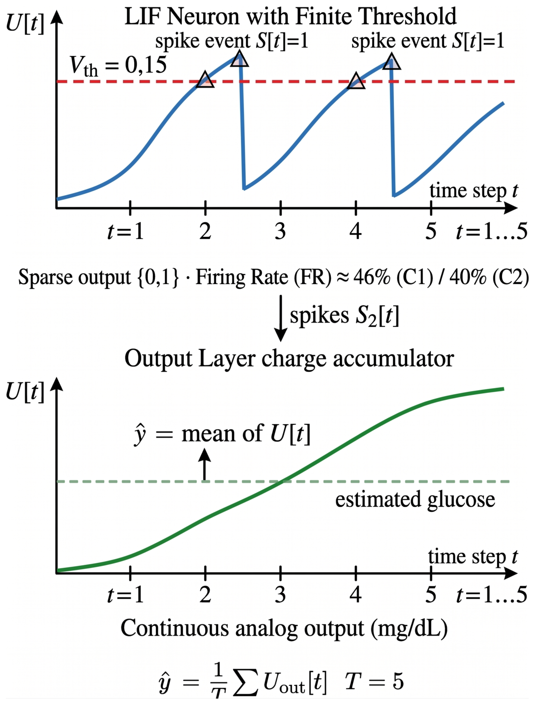
Figure 2.
Five-fold walk-forward cross-validation scheme. Each bar represents a patient’s time series split into training (blue), validation (orange) and unused period (gray). Fold 5 (★), with an 80%/20% split, is the principal reported result; the others provide statistical robustness estimates. All patients are present in both the training and validation sets of each fold.
Figure 2.
Five-fold walk-forward cross-validation scheme. Each bar represents a patient’s time series split into training (blue), validation (orange) and unused period (gray). Fold 5 (★), with an 80%/20% split, is the principal reported result; the others provide statistical robustness estimates. All patients are present in both the training and validation sets of each fold.
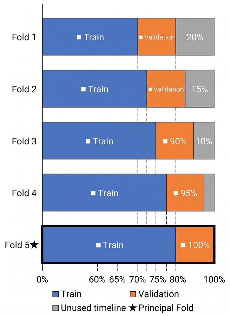
Figure 3.
LIF neuron dynamics in the two architectural configurations. Top—hidden layers (, ): the potential rises until it crosses the threshold, fires a spike (, orange triangles) and undergoes subtractive reset, producing sparse output. Bottom—output layer (, , no reset): the potential accumulates continuously and its temporal mean directly represents the estimated glucose in mg/dL.
Figure 3.
LIF neuron dynamics in the two architectural configurations. Top—hidden layers (, ): the potential rises until it crosses the threshold, fires a spike (, orange triangles) and undergoes subtractive reset, producing sparse output. Bottom—output layer (, , no reset): the potential accumulates continuously and its temporal mean directly represents the estimated glucose in mg/dL.
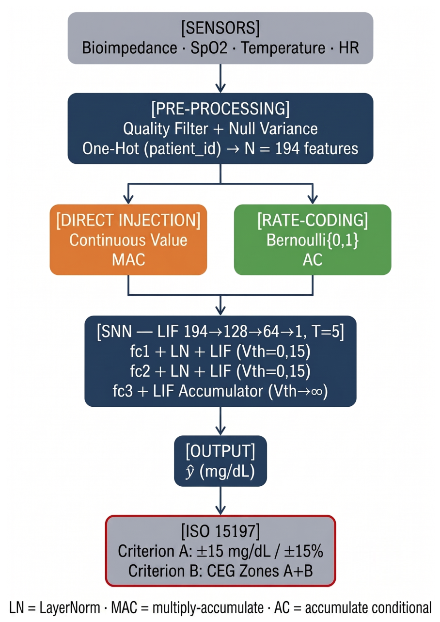
Figure 4.
Consensus Error Grid (ISO 15197:2013) of the Direct Injection variant () in fold 5: 100% of samples in Zones A+B.
Figure 4.
Consensus Error Grid (ISO 15197:2013) of the Direct Injection variant () in fold 5: 100% of samples in Zones A+B.
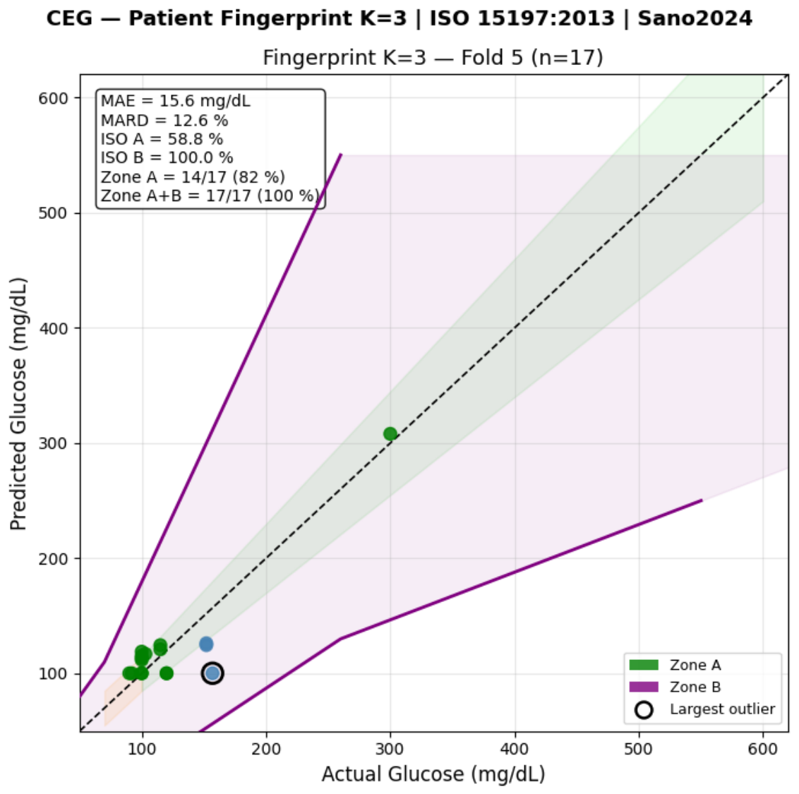
Figure 5.
Consensus Error Grid (ISO 15197:2013) of the Rate-Coding variant () in fold 5. The sparse encoding shows a slight clinical-safety degradation (ISO B = 98.8% averaged over folds) relative to direct injection (Figure 4).
Figure 5.
Consensus Error Grid (ISO 15197:2013) of the Rate-Coding variant () in fold 5. The sparse encoding shows a slight clinical-safety degradation (ISO B = 98.8% averaged over folds) relative to direct injection (Figure 4).
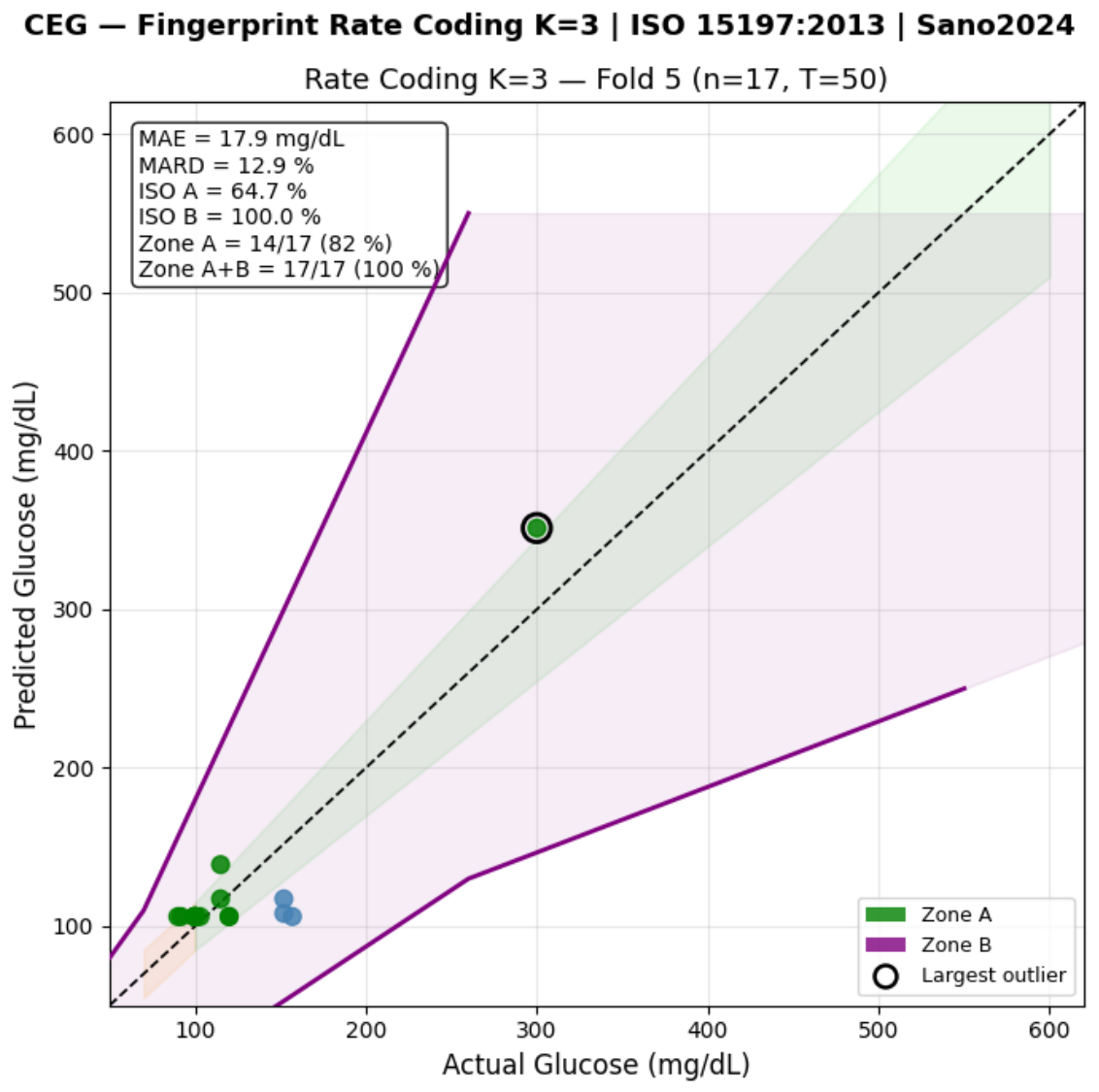

Table 1.
Cohorts derived from the 98-patient/717-measurement base.
| Cohort | Pat. | Meas. | Use in the Study |
|---|---|---|---|
| Base (preliminary) | 98 | 717 | Classification, SVR, encoding |
| sano2024 | 29 | 336 | Champion; importance; transfer (source) |
| 2024 broad (sensor) | 66 | 573 | Scalability |
| ICU2025 | 29 | 126 | Transfer (target) |
Table 2.
Overview of patient-calibration strategies on the 29-patient cohort (mean ± SD, 5 folds). All use end-to-end LIF regression with direct injection, except the last (rate-coding).
Table 2.
Overview of patient-calibration strategies on the 29-patient cohort (mean ± SD, 5 folds). All use end-to-end LIF regression with direct injection, except the last (rate-coding).
| Strategy | MAE (mg/dL) | MARD (%) | ISO A (%) | ISO B (%) |
|---|---|---|---|---|
| No calibration | 24.6 | 32.3 | 95.1 | |
| Offset () | 14.3 | 66.2 | 100 | |
| One-hot | 11.4 | 79.4 | 100 | |
| Fingerprint (injection) | 11.4 | 64.3 | 100 | |
| Fingerprint (rate-coding) | 13.5 | 75.1 | 98.8 |
Table 3.
The two embeddable fingerprint variants, each at its best K (mean ± SD, 5 folds; , 33,793 parameters).
Table 3.
The two embeddable fingerprint variants, each at its best K (mean ± SD, 5 folds; , 33,793 parameters).
| Metric | Direct Injection () | Rate-Coding (, ) |
|---|---|---|
| L1 encoding | Analog (MAC) | Bernoulli (AC) |
| MAE (mg/dL) | ||
| RMSE (mg/dL) | ||
| MARD (%) | 11.4 | 13.5 |
| R2 | 0.648 | 0.561 |
| ISO A (%) | 64.3 | 75.1 |
| ISO B—CEG (%) | 100 | 98.8 |
| Timesteps/inference | 5 | 50 |
Table 4.
Permutation importance (ΔMAE, mg/dL) of clinical features in two regimes—29-patient cohort. Global ranking position in parentheses.
Table 4.
Permutation importance (ΔMAE, mg/dL) of clinical features in two regimes—29-patient cohort. Global ranking position in parentheses.
| Clinical Feature | No History (Pointwise) | With History (Temporal) |
|---|---|---|
| Sex | (#1) | (#128) |
| Age | (#2) | (#26) |
| Diabetes type | (#3) | (#4) |
| BMI | (#28) | (#10) |
Table 5.
Permutation importance in the temporal model (29-patient cohort, fold 5, ). ID: identity (one-hot); C: clinical; S: sensor.
Table 5.
Permutation importance in the temporal model (29-patient cohort, fold 5, ). ID: identity (one-hot); C: clinical; S: sensor.
| Feature | Type | Rank | ΔMAE (mg/dL) |
|---|---|---|---|
| patient_24b… | ID | #1 | 6.80 |
| patient_394… | ID | #2 | 4.34 |
| maxled3 | S | #3 | 1.74 |
| diabetes type | C | #4 | 1.55 |
| bmi | C | #10 | 0.53 |
| age | C | #26 | 0.12 |
| sex | C | #128 |
Table 6.
Cross-cohort transfer—fingerprint trained on sano2024, evaluated on ICU2025.
| Scenario | MAE (mg/dL) | ISO B (%) |
|---|---|---|
| Intra-cohort (sano2024) | 100 | |
| Direct training on ICU | 88.3 | |
| Zero-shot transfer sano→ICU | 117.6 | 53.7 |
Table 7.
Comparison with the predecessor work (Cruz Castañeda and Bertemes Filho, 2024). SNN values refer to walk-forward 5-fold cross-validation (mean) over the full glycemic range.
Table 7.
Comparison with the predecessor work (Cruz Castañeda and Bertemes Filho, 2024). SNN values refer to walk-forward 5-fold cross-validation (mean) over the full glycemic range.
| Aspect | CatBoost (2024) | SNN (This Work) |
|---|---|---|
| Inference location | Cloud (CLL) | Edge (MCU) |
| R2 (5-fold mean) | 0.31 | 0.65 (0.83 fold 5) |
| RMSE (mg/dL) | 27.97 | |
| ISO 15197 validation | Not reported | Yes (Crit. A and B) |
| Latency under load | up to 3737 ms | local (no network) |
| Failure under load (50 users) | 11.46% | — |
| Embedded footprint | n/a (cloud) | ≈131 KB |
Disclaimer/Publisher’s Note: The statements, opinions and data contained in all publications are solely those of the individual author(s) and contributor(s) and not of MDPI and/or the editor(s). MDPI and/or the editor(s) disclaim responsibility for any injury to people or property resulting from any ideas, methods, instructions or products referred to in the content. |
© 2026 by the authors. Licensee MDPI, Basel, Switzerland. This article is an open access article distributed under the terms and conditions of the Creative Commons Attribution (CC BY) license (http://creativecommons.org/licenses/by/4.0/).
Copyright: This open access article is published under a Creative Commons CC BY 4.0 license, which permit the free download, distribution, and reuse, provided that the author and preprint are cited in any reuse.


