

Submitted:
22 July 2026
Posted:
23 July 2026
You are already at the latest version
Abstract
Prioritizing cows for closer observation around calving is important for livestock management, but reliable same-day calving detection from behavior alone remains challenging. We examine whether daily 06:00–06:00 behavior summaries derived from ear-tag accelerometers can support strictly causal, calving-oriented triage in grazing cattle. Because birth annotations provide only daily-resolution supervision, we frame the task as weakly supervised day-level risk assessment rather than precise event timing. Therefore, we train a compact weakly supervised multilayer-perceptron daily-risk model using an exactly-one likelihood over a two-day candidate window comprising the day before birth and the recorded day of birth. The model uses current behavior summaries, deviations from cow-specific causal behavior baselines for the current and previous retained days, a history-gap variable, and missingness indicators. We evaluate the model using cow-grouped nested cross-validation on data from 134 calving cows and 4,891 cow-days. At the primary base operating point, pooled out-of-fold predictions show a measurable but modest signal, with F1 score 0.277, MCC 0.244, AUPRC 0.231, and candidate-window detection 47.0%. Comparator methods recover similar signals with different detection–burden trade-offs: a supervised positive-bag random forest improves F1 score and candidate-window detection, but increases non-candidate false-alert burden. A higher-threshold Alert state reduces the retained non-candidate false-alert rate to 0.0121, but lowers recall to 0.194. Applying the frozen deployment model to an independent non-calving cohort yields low daily Watch/Alert rates but non-negligible cow-level exposure. Overall, daily behavior summaries are better suited to lightweight herd-level risk stratification and human-in-the-loop monitoring than to reliable standalone calving detection.
Keywords:
ear-tag accelerometer
; cattle
; calving monitoring
; weakly supervised learning
; decision support
1. Introduction
Timely supervision around calving is important for both animal welfare and farm management. Accurate birth-date information is also valuable for herd recording and genetic evaluation, including age adjustment of performance traits [1]. Delayed or missed intervention during abnormal parturition can increase the risk of dystocia-related complications, calf morbidity and mortality, postpartum health disorders, and adverse production and fertility outcomes [2,3,4,5]. These risks have motivated sustained interest in automated calving-monitoring technologies that help producers identify animals requiring closer observation during this critical period [4,6]. Proposed approaches include temperature sensors, tail-mounted devices, activity and rumination monitors, localization systems, accelerometers, and broader multi-sensor platforms, each offering a different balance among informativeness, practicality, and operational complexity [5,6].
Most existing cattle studies focus on dairy or relatively intensive settings, where high-frequency behavioral or physiological streams support calving-onset, calving-date, or time-to-calving prediction over horizons ranging from several days to only a few hours before calving [7,8,9,10,11,12,13]. For example, Rutten et al. [7] combined activity, rumination, ear temperature, and expected calving date to predict the start of calving in dairy cows; Krieger et al. [8] studied an ear-attached accelerometer in dairy cows; Miller et al. [9] evaluated animal-mounted tail and behavior-monitoring sensors in beef and dairy cattle and found that tail-sensor data alone provided useful time-to-calving prediction; and Liseune et al. [11] used sequential multivariate behavioral sensor data and deep learning to predict calving within windows from 24 h to 1 h. Other work evaluates complementary sensing configurations, including indoor localization with neck- and leg-mounted accelerometers for calving and estrus detection [14], and automated tail-movement monitoring combined with rumination time and behavioral observations for identifying calving time [15]. Collectively, these studies show that behavioral change around calving is informative, consistent with observational evidence of reduced rumination and feeding around parturition [16,17]. However, many existing systems target short-horizon onset prediction, rely on specialized sensing or close-range infrastructure, or are evaluated in management contexts that differ substantially from broad-acre grazing operations.
Small-ruminant parturition monitoring provides closely related evidence that wearable sensors can capture pre-parturition activity and behavioral changes relevant to lambing or kidding detection [18,19,20]. Recent deployment-aware studies have also considered how sampling rate, history-window length, model complexity, and sensor configuration affect parturition-detection performance in sheep and goats [21,22]. These studies reinforce the practical value of resource-aware wearable monitoring in grazing and extensive production settings. However, many of these studies use higher-frequency sensor streams, shorter decision windows, or more temporally detailed parturition labels than the daily cattle behavior summaries available in the present calving study.
This distinction becomes especially important when moving from intensive dairy environments to extensive grazing and rangeland systems. In such settings, labor is often limited, animals are spatially dispersed, and sensing solutions must remain lightweight, durable, and easy to integrate into routine management. Among the more relevant studies in extensive systems, García García et al. [23] investigated calving detection from GNSS-collar data in beef cows grazing on rangelands, while Wang et al. [24] proposed a two-stage machine-learning pipeline for rangeland cattle using a low-power IoT platform that combines GNSS and tri-axial accelerometers. In the latter study, the authors first used an autoencoder with time encoding to flag anomalous behavior and then applied a random-forest classifier to distinguish calving-related anomalies from other anomalies. That work is close to our target domain in its extensive-management focus, but it uses richer real-time raw sensor streams and frames the task primarily as anomaly-driven event detection. By contrast, we start from daily behavior summaries derived from ear-tag accelerometers and ask a more constrained deployment-oriented question: given only the information available up to the current day, can we produce a useful same-day calving-oriented triage signal?
This change in temporal resolution alters the learning problem. Once behavior is aggregated into daily 06:00–06:00 summaries, the input no longer represents calving as a sharply timed event. The recorded day of birth (DoB) may align imperfectly with the most informative behavioral day, especially when parturition occurs near the aggregation boundary. The resulting day-level label is therefore intrinsically uncertain relative to the behavioral window. Rather than treating this mismatch as incidental noise, we incorporate it into the problem formulation. The nature of this task connects it to weakly supervised and multiple-instance learning: each calving cow provides a small candidate set of plausible event days, but the available daily-resolution label does not identify which day contains the strongest calving-related behavioral expression [25].
This perspective also clarifies how our work differs from prior calving-prediction studies. We do not aim to provide precise hour-level onset prediction, retrospective localization of the calving event, or high-resolution alarms from raw multimodal streams. Instead, we investigate what calving-relevant information can be inferred from deployment-friendly daily behavior summaries that may already be available from scalable ear-tag monitoring systems, and how such information can support practical triage rather than exact event detection. Ear-tag accelerometers are attractive in this context because they fit naturally within routine livestock-monitoring workflows, and accelerometers more broadly are among the most widely used wearable sensors for ruminant behavior analysis [26,27,28]. Recent studies have shown that ear-tag accelerometers can support automated rumination detection and broader behavior prediction [29,30], and that accelerometer-derived behavior profiles can support livestock behavior forecasting and missing-data imputation with modern sequence models [31]. Importantly for calving-oriented monitoring, accelerometer-derived rumination patterns also change around parturition [17]. These observations suggest that daily summaries derived from ear-based sensing may retain useful reproductive-state information, even if they are too coarse for precise event timing.
Accordingly, we evaluate whether daily 06:00–06:00 behavior summaries derived from ear-tag accelerometers can support strictly causal, calving-oriented triage in grazing cattle. Our primary model is a compact multilayer perceptron (MLP) that outputs a daily calving-risk score from a strictly causal feature representation. This representation includes raw daily behavior summaries, current and previous-retained-day deviations from cow-specific causal behavior baselines, a history-gap variable, and missingness indicators. We handle ambiguous day-level supervision explicitly through a weakly supervised exactly-one formulation and evaluate the resulting scores together with simple deployment-oriented triage rules. To place this formulation in context, we compare it with a weak exactly-one logistic-regression model, supervised positive-bag classifiers trained on the same primary feature representation, and simple causal deviation-threshold rule methods. We also report supporting ablations over raw-only, deviation-only, raw-plus-deviation, lagged-deviation, and longer-history feature variants, together with sensitivity analyses for missingness handling, candidate-window definition, and operating-threshold selection.
We focus on a strictly causal deployment setting in which each daily prediction must be made without future information or retrospective relabeling. The framework converts daily risk estimates into Low, Watch, and Alert states intended to support practical observation and inspection decisions under field conditions. To further characterize operational burden, we also apply the frozen exported model to an independent non-calving cohort collected during a separate estrus-monitoring study, treating this analysis as an out-of-domain burden check rather than as a matched calving-specificity validation. More specifically, we make the following contributions:
- We formulate calving-oriented monitoring under daily behavioral aggregation as a strictly causal, weakly supervised, day-level triage problem, where the candidate window includes the day before birth and the recorded DoB.
- We propose an exactly-one weakly supervised likelihood over the candidate window and use it to train a compact MLP on a strictly causal feature set comprising daily behavior summaries, current and previous-retained-day baseline-referenced behavior deviations, a history-gap variable, and missingness indicators.
- We evaluate the proposed model using cow-grouped nested cross-validation on a dataset comprising 134 calving cows and 4,891 cow-days, and benchmark it against a weak exactly-one logistic-regression model, supervised positive-bag classifiers, and deviation-based rule methods.
- We map daily risk scores from the trained MLP to a three-state Low/Watch/Alert triage output using base thresholds selected only from training data and prespecified triage rules, and quantify the resulting trade-off among precision, candidate-window detection, and false-alert burden.
- We perform an out-of-domain burden check by applying the frozen deployment model to an independent non-calving cohort, while explicitly discussing the interpretive limits of this analysis.
- We delineate the operating ceiling imposed by daily aggregation, weak labels, and dependence on upstream behavior classification, and identify sensing and supervision upgrades likely needed for autonomous calving detection.
2. Data
We describe the two datasets used in this study, the available reproductive annotations, and the preprocessing steps used to construct model-ready daily behavior records. Both datasets are represented as daily 06:00–06:00 behavior summaries derived from ear-tag accelerometer readings.
2.1. Main Calving Study
We use a primary dataset collected during a field trial at Nindooinbah1, a commercial seedstock cattle operation near Beaudesert in the Scenic Rim Region of Queensland, Australia, from 21 October to 1 December 2025. The retained 06:00–06:00 behavioral days span 22 October to 30 November 2025. The trial enrolled 181 Angus, Brangus, and Ultrablack cows managed under commercial field conditions that included grazing and feedlot components (see Figure 1).
Each animal wore a CERES RANCHER ear-tag2 containing a triaxial accelerometer. An upstream behavior-classification pipeline first predicted behavior at finer temporal resolution using the classifier described by Arablouei et al. [32], and then aggregated the predicted labels into fixed 06:00–06:00 behavioral days. For each cow-day, the available summary contains the total daily duration of grazing, walking, ruminating, resting, and a residual “other” class for behavior not assigned to those four categories. We express behavior summaries as daily hours, with the five behavior durations summing approximately to 24 h for each retained cow-day. We use these 06:00–06:00 daily summaries as the only behavioral inputs for all subsequent feature construction and risk modeling.
2.2. Calving Annotations
For each cow in the main study, we use the field-recorded DoB. This annotation anchors the event at daily resolution, but it does not identify the exact time of parturition within the 06:00–06:00 behavioral day used for modeling. In practice, calving rounds occurred once daily in the morning, at times that could vary, so a calf recorded on a given DoB may have been born up to approximately 24 h earlier. As a result, the daily summary most affected by calving may plausibly correspond either to the recorded DoB or to the preceding behavioral day.
To make this uncertainty explicit, we treat the calving label as weak at the day level and define the candidate calving window as the two-day set , comprising the day before birth and the recorded DoB, as illustrated in Figure 2. This choice is part of the problem formulation rather than a post hoc relabeling rule, reflecting the mismatch between field-recorded calving event dates and fixed daily behavior aggregation windows.
This day-level ambiguity is also consistent with practical field recording in grazing systems, where calving dates are typically established from routine observation or farm records rather than exact time-stamped event annotations. Additional uncertainty may arise from delayed calf discovery or the timing of inspection rounds, which further supports treating the day assignment as weak at 24 h resolution.
2.3. Preprocessing and Retained Analysis Set
We screened daily behavior summaries for availability and quality before modeling. We retained only behavioral days with at least 95% expected prediction-window coverage and excluded days with more than 16 h classified as resting. The first rule removes days with insufficient sensor coverage, which can occur when an ear tag stops operating or transmitting data. In this trial, such interruptions were rare and often associated with battery depletion caused by continuous transmission of high-volume raw accelerometer data over an LTE network as part of research data collection. This raw-data streaming mode is not required for routine deployment, where substantially smaller behavior-summary outputs would be transmitted instead. The second rule removes days with implausibly high resting time, which may occur when a device was not yet deployed, had been removed from the animal, or was no longer recording representative behavior, including after animal mortality.
These day-level quality-control steps also affected cow-level inclusion. Although the field trial enrolled 181 cows, some cows had no retained daily behavior records that were useful for the present calving-monitoring analysis after annotation alignment and preprocessing. We therefore restricted the modeling dataset to cows with usable retained behavioral data for the analysis period. We did not exclude any additional cows merely because early history-dependent features were unavailable.
Some early retained cow-days had insufficient prior history to compute all temporal features used later in the model. We retained these records rather than discarding them and handled unavailable derived values during model training using missingness-aware preprocessing.
After preprocessing, the retained analysis dataset includes 134 calving cows and 4,891 cow-days, corresponding to an average of 36.5 analyzed days per cow. The default candidate window contributes 268 candidate-window cow-days, and the remaining 4,623 retained cow-days are non-candidate days used to estimate off-window false-alert burden. These non-candidate records comprise 1,232 cow-days before the candidate window and 3,391 cow-days after the candidate window. Of all retained cow-days, 4,355 have complete continuous components for the primary feature set defined in Section 3.4, and 536 have at least one unavailable history-dependent component but remain in the analysis.
2.4. Independent Non-Calving Cohort for Burden Assessment
To examine how the learned calving-oriented signal behaves outside the original calving cohort, we also use an independent non-calving cohort from a separate estrus-monitoring study in grazing cattle at the CSIRO Chiswick Research Station, Armidale, NSW, Australia [32]. No cows calved during this experiment. After alignment to the daily 06:00–06:00 behavior summaries used in this study, the retained external scoring dataset comprises 31 cows and 1,547 scored cow-days, spanning behavior-day dates from 31 January 2025 to 7 May 2025.
As in the main study, each cow has daily 06:00–06:00 summaries of grazing, walking, ruminating, resting, and other behavior. We do not use the external dataset for model training, model selection, threshold tuning, or recalibration. Instead, we apply the final deployment model, trained on the full calving development dataset, unchanged, to the external daily behavior summaries. This analysis quantifies out-of-domain score and triage-output burden in a separate non-calving cohort, rather than estimating estrus-detection performance or matched calving specificity.
2.5. Ethics and Animal Care
We collected all data under approved institutional animal-care procedures. Farm staff managed the animals according to standard farm practices. The study team attached the ear-tags carefully and in accordance with relevant animal-welfare guidelines to minimize disturbance and discomfort. After deployment, data retrieval did not require repeated animal handling because sensor data was transferred through Bluetooth gateways and the LTE network. The CSIRO Livestock Animal Ethics Committee approved the main calving study under Animal Research Authority (ARA) 25/05 and the estrus study that provided the independent non-calving cohort under ARA 24/11.
2.6. Summary of Data Used in This Study
Table 1 summarizes key statistics for the two datasets used in this study. Both datasets are represented as 06:00–06:00 daily behavior-summary records derived from ear-tag accelerometer data from grazing cattle. We use the main calving dataset for model development, internal evaluation, and operating-threshold selection. We use the independent non-calving cohort only for external scoring of the frozen deployment model and summarizing out-of-domain triage burden.
3. Methods
In this section, we define the proposed calving-monitoring pipeline, including daily behavior representation, causal baseline and lagged-deviation feature construction, weakly supervised model training, threshold selection, triage mapping, deployment implementation, and evaluation measures. Figure 3 summarizes the full pipeline.
3.1. Overview
The methodological design follows directly from the deployment setting introduced in Section 1 and the annotation structure described in Section 2. At the end of each 06:00–06:00 behavioral day, the system has access only to that cow’s current daily behavior summary and recent behavioral history. It cannot observe future days or the exact within-day time of calving. We use field-recorded reproductive annotations for training and evaluation, but not as online inputs. The resulting task is therefore a strictly causal, weakly supervised, day-level risk-assessment problem rather than a precise event-timing problem.
The proposed framework has two components. First, a weakly supervised daily-risk model maps features derived from daily behavior summaries to a calving-oriented score for each cow-day. Second, causal decision rules convert this score into an operational Low, Watch, or Alert state intended to support field monitoring. The aim is not retrospective event localization, but same-day prioritization of observation and inspection under realistic information constraints.
3.2. Daily Behavior Summaries
For cow i and behavioral day t, we use behavior predictions aggregated over a 24 h 06:00–06:00 window, indexed by the calendar date of the starting 06:00. We denote the resulting daily behavior vector by
where , , , , and are the daily durations of grazing, walking, ruminating, resting, and other behavior, respectively. We treat the other class as a residual behavior category covering predicted states not assigned to the four named behaviors.
The upstream pipeline obtains these daily summaries by first applying the classifier described by Arablouei et al. [32] to 5.12 s windows, and then aggregating the predicted labels over each 24 h behavioral day. We use this classifier only as an upstream source of standardized daily behavior summaries. The calving-oriented model developed here operates entirely at daily resolution.
Our calving-monitoring approach does not rely on the raw daily summaries alone. Instead, it augments the current-day behavior profile with causal deviation-from-baseline values, previous-day deviation values, a history-gap variable, and missingness indicators. This design reflects both the biological motivation for the problem and the practical need to track behavioral changes in each cow relative to its own recent behavior rather than a population-level average.
3.3. Causal Behavioral Baselines
For each cow i, behavior class , and behavioral day t, we construct a cow-specific causal baseline using historical observations from a fixed lookback window of W days preceding day t. Let denote the component of the daily behavior vector corresponding to behavior class b. The baseline window spans days to , subject to data availability. In this study, we use .
We define the set of available historical values within this window as
Let denote the number of valid historical observations. Sorting the elements of in ascending order yields the order statistics
To reduce the influence of short-term anomalies while retaining as many usable historical values as possible, we compute the causal baseline using an adaptive trimmed mean:
Figure 4 illustrates this causal baseline construction for a single behavior class.
Using this baseline, we define the behavioral deviation for cow i, behavior class b, and day t as
If the baseline is missing because of insufficient historical data (), the corresponding deviation is also marked as missing. We propagate these missing values through the feature pipeline and explicitly encode them using binary missingness indicators in the downstream model.
To provide descriptive intuition for the baseline-referenced feature design, Figure 5 aligns daily deviation summaries by recorded DoB and summarizes the resulting distributions across cows. We use this retrospective visualization only to motivate the feature construction. At deployment, the model does not observe future information or aligned event time. Despite substantial between-cow variability, the aligned deviations reveal a coherent peri-calving pattern, most notably a pronounced decrease in rumination around the candidate window , together with smaller shifts in grazing, resting, walking, and other behaviors. These descriptive patterns support the use of cow-specific deviation-from-baseline features rather than reliance on absolute daily behavior summaries alone.
3.4. Primary Strictly Causal Behavioral Features
Let
denote the deviation vector for cow i on retained 06:00–06:00 behavioral day t, where each component represents the departure of a daily behavior duration from its cow-specific causal baseline. Because these baselines are constructed using only historical summaries, the resulting features remain strictly causal. Calendar dates are used only to index these behavioral days and preserve day-level spacing when computing baselines and history gaps.
Our primary feature representation is
where is the current daily behavior vector, is the current deviation vector, and is the deviation vector from the cow’s previous retained behavioral day. The scalar records the elapsed number of days between the current and previous retained records. If no prior retained record exists, both and are marked as missing before imputation.
The binary vector records feature missingness, with indicators for the five components of , the five components of , and the scalar . Each entry is set to 1 if the corresponding feature is missing before imputation and 0 otherwise. Thus, comprises 16 continuous variables and 11 binary indicators, yielding a processed model-input dimension of 27 after concatenation.
This design integrates absolute daily behavior durations, current deviations from baseline, previous retained-day deviations, and missingness bookkeeping into a single strictly causal representation. Conceptually, it allows the downstream model to account for absolute behavior levels, recent cow-specific departures from baseline, and the availability of the short history needed to form those comparisons. We adopt this configuration as the primary feature set because it is informative while remaining computationally compact for deployment.
For completeness, we also evaluate several alternative causal feature sets as ablations. To keep the main text focused on the primary representation, we define and compare these alternatives in Appendix A.
3.5. Weakly Supervised Daily-Risk Model
The daily labels in our calving dataset are weak rather than exact. Farm staff checked for calving once daily in the morning, at times that could vary, hence the recorded DoB reflects the day on which the calf was observed rather than an exact parturition timestamp. Because the data pipeline also aggregates behavior predictions over fixed 06:00–06:00 windows, the recorded DoB does not identify which behavioral day is most closely aligned with the calving event. Therefore, we define the candidate calving window for cow i in relative-day coordinates as
where day denotes the 06:00–06:00 behavioral day preceding the recorded DoB and day 0 denotes the 06:00–06:00 behavioral day indexed by the recorded DoB. The central modeling assumption is that one of these two behavioral days contains the latent calving event, although the training data does not identify which one.
Let denote the model logit for cow i on relative day t, where is the strictly causal feature vector and represents the model parameters. The corresponding day-level score is
where is the logistic sigmoid function. We interpret as a calving-compatibility score: higher values indicate that the behavior on day t is more consistent with the latent calving day under the weak-supervision formulation. During deployment, these scores are computed causally for each cow-day and then mapped to operational monitoring states.
For training and evaluation, we treat all retained scored days outside the candidate window as non-candidate examples. We do not impose an exclusion zone around . Consequently, near-event days outside remain in the analysis as non-candidate days. Let denote the set of retained non-candidate days for cow i, and let
denote the corresponding set of retained non-candidate cow-days across the analyzed herd .
To model the latent assignment within , we use an exactly-one weakly supervised likelihood. Under an independent Bernoulli scoring model for the candidate days, the probability that exactly one candidate day is positive for cow i is
For the two-day candidate window , this reduces to
This likelihood reflects the annotation ambiguity in our setting: the recorded DoB and fixed 06:00–06:00 aggregation identify a two-day candidate window, but not which of the two behavioral days contains the latent calving event.
The exactly-one formulation is deliberately conservative. A standard positive-bag or at-least-one multiple-instance learning formulation allows both candidate days to receive high scores. Such a formulation may be appropriate for broader periparturient-risk tracking, but it is less aligned with our immediate objective of deciding whether a specific daily summary warrants same-day management attention. Therefore, we use the exactly-one formulation as the primary weakly supervised model and treat its output as a behavioral compatibility score rather than a calibrated probability of calving.
The model training objective is the joint negative log-likelihood
where is a numerical stabilizer and controls the penalty on non-candidate days. The first term encourages the model to assign a high score to exactly one day in each candidate window, while the second term suppresses elevated scores on retained non-candidate days. At inference, the fitted model is applied sequentially to produce a daily risk-score stream, which is then mapped to Low, Watch, and Alert management states.
3.6. Model Architecture and Training
To map the causal feature representation to a day-level calving-compatibility score, we use a compact feed-forward neural network, namely a multilayer perceptron (MLP) with one hidden layer. Let denote the preprocessed model input constructed from . The model output is
where is the logistic sigmoid function, and are the hidden-layer and output-layer weights, and and are the corresponding biases. This architecture provides a parsimonious nonlinear scorer that can capture interactions among daily behavior durations, baseline-referenced deviations, and missingness indicators without introducing excessive capacity relative to the available sample size.
We compute using a strict data-isolation protocol. Missing values in the continuous features are imputed using medians computed only from the active training fold. The imputed continuous features are then standardized using the corresponding training-fold means and standard deviations, after which we append the 11 binary missingness indicators unchanged. This allows the model to distinguish unavailable history from observed values near the imputed median, which is especially important during the initial days of a cow’s retained time series when lagged or baseline-derived features are causally undefined.
We estimate the trainable parameters by minimizing the weakly supervised objective defined in Section 3.5 using the Adam optimizer [33] with a learning rate of and weight decay of . We train each model for up to 600 epochs, with early stopping after 80 epochs without improvement in the training objective. Given the moderate size of the training data, we use full-batch optimization rather than stochastic mini-batching to obtain stable gradient updates.
We determine the hidden-layer width using the automatic rule , where is the number of continuous non-mask input features. For the primary feature representation , this gives . We tune the non-candidate-day penalty weight over within the cow-grouped nested cross-validation procedure described in Section 3.7. We select the operating threshold separately using the procedure described in Section 3.9.
3.7. Cross-Validation
We obtain the results on the calving dataset using cow-grouped nested cross-validation, so that all days from a given animal remain in the same fold. This prevents information leakage across days from the same individual and ensures that each held-out fold represents unseen animals rather than unseen days from animals already observed during training.
Specifically, we use four outer folds for held-out evaluation and three inner folds within each outer training split. Within this nested structure, all preprocessing steps, including median imputation and standardization, are fitted using training data only, and the non-candidate-day penalty weight and operating threshold are selected without access to the corresponding held-out outer-fold animals. This design provides a cleaner estimate of how the proposed system would behave when applied to new cows under the same deployment setting.
We use this cow-grouped nested cross-validation protocol for all results based on the main calving dataset. We do not cross-validate the independent non-calving estrus cohort. Instead, we use it only as an external scoring check of the frozen calving-oriented Watch/Alert tool.
3.8. Comparator Methods
To evaluate the utility of the weakly supervised exactly-one formulation and the nonlinear MLP parameterization, we compare the primary model with three classes of comparator methods using the same retained cow-days. First, we include a weak exactly-one logistic-regression comparator. It uses the same primary feature representation and exactly-one weak-supervision likelihood as the MLP, but replaces the hidden-layer network with a linear logistic score. This comparator separates the contribution of the weak-supervision formulation from the contribution of the nonlinear hidden-layer parameterization. We tune its non-candidate-day penalty weight over and select its operating threshold within the same cow-grouped inner cross-validation framework used for the primary model.
Second, we train standard supervised classifiers on the primary feature representation, treating both days in the candidate window as positive instances and all retained non-candidate days as negative instances. This replaces the latent event-day assignment objective with ordinary binary classification on the same causal inputs, providing a direct reference for assessing whether explicitly modeling event-day uncertainty improves the learned daily-risk score. We evaluate logistic regression, random forest, and XGBoost classifiers. For each classifier type, hyperparameters and operating thresholds are selected within the cow-grouped inner cross-validation loop, with final predictions obtained on the held-out outer folds. For logistic regression, we tune the regularization strength over . For random forest, we use 100 trees and evaluate all combinations of maximum depth in and minimum leaf size in . For XGBoost, we evaluate all combinations of , learning rate in , and maximum depth in , while fixing both row and column subsampling at . We keep these grids deliberately compact to limit overfitting given the modest number of animals available for grouped evaluation.
Third, we evaluate simple, unlearned causal rules derived from current behavioral deviations. Let denote the current deviation after missing values are imputed using the training-split median and subsequently standardized using the training-split mean and standard deviation for behavior channel b. This preprocessing follows the same strict data-isolation protocol used for the learned models, but is applied only to the current deviation features required by the heuristic rules. We define three rule scores: a rumination-drop score,
a directional peri-calving deviation score,
and a maximum absolute-deviation score,
where denote grazing, walking, ruminating, resting, and other, respectively. The directional rule captures the descriptive peri-calving pattern of reduced rumination together with possible increases in walking or resting, without requiring a learned classifier. Each heuristic produces a continuous daily score, with its operational threshold selected within the same inner cross-validation structure. These rules are not intended as optimized production systems. Rather, they provide transparent references for assessing whether the learned models justify their additional complexity over simple deviation-threshold heuristics.
3.9. Risk-Score Thresholding and Triage States
After model training, each retained cow-day receives a causal daily score . Because the system is designed for observation prioritization rather than autonomous calving declaration, we treat as a relative ranking score rather than a calibrated probability. Let denote the most recent previously scored retained behavioral day for cow i. All thresholding and triage operations are applied independently within each cow’s scored time series.
We first select a base operating threshold within the training portion of each outer fold using the candidate grid . We choose the threshold that maximizes the inner-validation F1 score, breaking ties first in favor of the lower retained non-candidate false-alert rate and then, if needed, the higher Matthews correlation coefficient (MCC). The F1 criterion provides a transparent default balance between precision and recall without requiring a deployment-specific cost model, while the tie-breaks favor lower off-window burden and deterministic selection. In deployment, this base threshold can be adjusted to match inspection capacity and risk tolerance.
During model training and evaluation, threshold selection never uses held-out outer-fold test data. For reproducibility, each model or comparator receives its own fold-specific base threshold selected using only the corresponding outer-training data through the inner-validation procedure.
Beyond direct thresholding of the raw score at , we also consider two diagnostic operating rules to separate the effects of score magnitude and temporal post-processing: a balanced rising rule, which requires and , and a quiet-3 rule, which requires and suppresses repeated alerts after recent alert-eligible scored records.
For the final operational output, we map the continuous score to three triage states relative to the fold-specific base threshold : Low, Watch, and Alert. The intermediate Watch state distinguishes lower-confidence upward score movements from higher-confidence Alert events that warrant immediate closer inspection. The daily states are defined as follows:
- Low: neither the Watch nor the Alert condition is satisfied.
-
Watch:This state flags days where the score is moderately elevated and strictly increasing relative to the previous scored retained behavioral day. If no previous scored record is available, the rising condition is false.
- Alert:provided that no alert-eligible record has occurred among the preceding three scored daily behavioral records for the same cow. This quiet-3 rule acts as a refractory mechanism that suppresses duplicate alerts during sustained high-score periods, reducing operational alert burden without changing the underlying score sequence.
When both conditions are satisfied, Alert takes precedence over Watch. Operationally, a Watch designation prompts heightened observation, whereas an Alert prompts immediate physical inspection.
The multipliers 0.9 and 1.2 are pragmatic default choices for this dataset rather than biological constants. In deployment, they can be adjusted along with to reflect local inspection capacity and risk tolerance. We examine sensitivity to these multiplier choices in Appendix C.
3.10. Performance Evaluation Measures
We evaluate the proposed method at two complementary levels. First, at the day level, we assess whether positive outputs concentrate on the ambiguous calving candidate days rather than on retained non-candidate days. Because the exact latent calving day within the candidate window is unobserved, day-level thresholded metrics treat both days in as candidate positives. These metrics therefore measure candidate-day enrichment rather than exact within-window calving-day localization. For binary outputs, we report precision, recall, F1 score, and MCC. Precision and recall characterize the false-alert–coverage trade-off of the alert stream, F1 provides a compact summary of that trade-off, and MCC is included because it uses all four entries of the confusion matrix and remains informative under the strong class imbalance induced by the small number of candidate-window days. To complement these threshold-dependent measures, we report the area under the precision–recall curve (AUPRC) for the raw daily scores. AUPRC provides a threshold-free summary of ranking quality under class imbalance, whereas the threshold-dependent measures characterize performance at the default operating point used for reproducible evaluation. We do not emphasize overall accuracy because, under the strong class imbalance in this dataset, it would be dominated by the much larger number of retained non-candidate cow-days.
Second, because the intended use case is operational triage rather than exact day assignment, we report cow-level detection and false-alert burden summaries. Candidate-window detection is the proportion of calving cows for which at least one positive output occurs in . For thresholded outputs, the false-alert rate is the proportion of retained non-candidate scored cow-days with a positive output. Because retained non-candidate days include both pre-candidate and post-candidate days, Appendix B reports a secondary diagnostic that separates the pooled false-alert burden into pre- and post-candidate components. Thus, candidate-window detection summarizes operational sensitivity at the cow level, whereas the false-alert rate summarizes off-window burden at the cow-day level.
This distinction is especially relevant for the weak exactly-one formulation. The exactly-one likelihood encourages the model to concentrate risk on one day within the two-day candidate window, whereas day-level recall treats both days in as positives. As a result, day-level recall is conservative for this model class: a cow can be operationally detected even if only one of the two candidate days is flagged. Therefore, we retain standard day-level performance measures for comparability across methods, but interpret candidate-window detection as the more deployment-aligned sensitivity measure.
When interpreting practical usefulness, we place the greatest weight on the combination of candidate-window detection and false-alert burden. A method with modest day-level discrimination may still be useful if it concentrates alerts into a small number of actionable inspection opportunities, whereas a method with slightly stronger internal classification scores but frequent off-window firing is less attractive operationally.
3.11. Deployment Implementation
The final deployment pipeline uses the same strictly causal preprocessing, risk-scoring, and triage logic as the development pipeline. After fitting the final model on the full calving dataset, we store the feature-wise imputation medians, scaling parameters, trained risk-model weights and biases, base threshold, and default Watch/Alert rules. For the frozen deployment model used in the independent non-calving estrus-cohort analysis, we use the primary feature representation in (1) and the same training protocol as in the nested cross-validation analysis. The hidden width is set by the predefined rule, giving for the 16 continuous non-mask inputs. We use weight decay , learning rate , a maximum of 600 epochs, and patience 80. We set for this frozen full-data model because it was the modal value selected across the four outer folds for the primary representation, occurring in three of the four nested cross-validation runs. We then retrain the final model on all retained calving-study data using this value. We set the stored base threshold to , the mean of the four outer-fold selected base thresholds for the primary feature set. This frozen deployment model has 262 trainable parameters and is used only for the independent non-calving cohort burden check. All reported internal calving-study performance estimates come from the cow-grouped nested cross-validation procedure.
For each cow i and each new 06:00–06:00 behavioral day t, deployment proceeds as follows:
- Compute the daily behavior summary .
- Construct the causal baseline-referenced deviation , retrieve the previous scored-record deviation , and compute the history-gap variable .
- For each unavailable derived component, impute its numeric value using the stored training-set median and set the corresponding missingness indicator to denote unavailable history.
- Apply the stored preprocessing transformation and evaluate the trained model to obtain the daily score .
- Convert into the corresponding Low, Watch, or Alert state using the default deployment rules.
This design preserves strict causality and keeps development-time evaluation consistent with online use. The missingness indicators serve only to distinguish unavailable history from observed temporal context, not to introduce additional behavioral information. As a result, the system can score the earliest retained days for each cow while still indicating when baseline or lagged features are unavailable.
4. Results
We organize the experimental results around the intended operational deployment of the proposed method. First, we report the cross-validated performance of the daily-risk model and its derived causal operating rules, and compare the primary weakly supervised MLP with a weak exactly-one logistic-regression model, supervised positive-bag classifiers, and heuristic rule-based methods. Second, we analyze the threshold-free and event-aligned behavior of the risk scores to clarify the constraints behind the observed operating trade-offs. Third, we summarize sensitivity to alternative feature sets, with full ablations deferred to the appendix. Finally, we evaluate the operational burden of the frozen deployment model through an out-of-domain check on an independent non-calving cohort.
Unless specified otherwise, we obtain the primary internal calving-study results by pooling held-out predictions across the four outer folds of the cow-grouped nested cross-validation protocol described in Section 3.7. We provide fold-level summaries, reported as mean ± standard deviation across outer folds, in Appendix D. Given the modest number of calving events and the four-fold cross-validation structure, we treat these evaluations as descriptive operating-point and burden analyses rather than formal hypothesis tests. Consequently, we do not report p-values or claim statistical superiority between methods. We report the external non-calving burden check separately and do not use it for model selection, threshold tuning, or recalibration.
4.1. Risk Model and Triage Operating Rules
We use the strictly causal representation in Eq. (1) to generate a daily calving-oriented risk score. For each outer fold, the raw-score operating threshold is selected using only the corresponding training data through the inner-validation procedure described in Section 3.9. We then apply the selected fold-specific threshold to the held-out predictions from that outer fold and pool the resulting predictions across folds for evaluation. Table 2 summarizes the internal out-of-fold performance of the base-thresholded raw score, the deployment-oriented operating rules, and the hard Alert state from the three-state triage output.
Applying the fold-selected base threshold directly to the raw daily-risk score achieves day-level precision, recall, F1 score, and MCC of , , , and , respectively. The corresponding AUPRC is , and the false-alert rate on retained non-candidate cow-days is . At the cow level, the model produces at least one positive day within the candidate window for of cows. These values indicate that the score contains useful peri-calving information, but direct base-thresholding does not yield a sufficiently clean or sensitive same-day detector.
The causal operating rules mainly shift this trade-off rather than changing it qualitatively. The balanced rising rule stays close to the base-thresholded score, with precision , recall , MCC , candidate-window detection of , and a false-alert rate of . The more conservative quiet-3 rule reduces the false-alert rate from to , but recall decreases to and candidate-window detection to .
The three-state triage formulation provides the cleanest strict inspection trigger. The hard Alert state reaches day-level precision of and reduces the false-alert rate on retained non-candidate cow-days to . This comes at the cost of lower recall () and lower candidate-window detection (). Therefore, we interpret the triage output as a prioritization signal: it provides a cleaner alert stream for follow-up checks, but it does not remove the sensitivity limitation inherent in the daily behavior signal.
4.2. Comparator-Method Performance
Table 3 compares three groups of alternatives to the primary weak exactly-one MLP. The weak-likelihood comparators isolate modeling choices within the weak-supervision framework: the weak at-least-one MLP keeps the same one-hidden-layer architecture but replaces the exactly-one candidate-window likelihood with an at-least-one likelihood, whereas the weak exactly-one LR keeps the exactly-one likelihood but uses a linear logistic score. The supervised positive-bag comparators treat both candidate-window days as positive and test whether standard classifiers can recover a useful day-level peri-calving risk signal. The rule-based comparators use causal deviation-derived scores motivated by the descriptive peri-calving behavior patterns.
Within the weak-likelihood group, the weak at-least-one MLP gives higher recall, F1 score, MCC, AUPRC, and candidate-window detection than the weak exactly-one MLP, but with a higher false-alert rate on retained non-candidate cow-days. This result suggests that allowing both candidate-window days to receive high scores can recover a stronger peri-calving risk signal, but with a less event-specific supervision model and slightly higher off-window burden. The weak exactly-one LR achieves higher precision and a lower false-alert rate than the weak exactly-one MLP, but at the cost of lower recall, AUPRC, and candidate-window detection. This pattern suggests that the compact nonlinear MLP improves sensitivity to the peri-calving signal relative to a linear exactly-one model, while retaining a moderate false-alert burden.
Among the supervised positive-bag comparators, random forest gives the strongest overall operating point, with the highest recall, F1 score, MCC, and candidate-window detection in this group. XGBoost gives a similar but slightly weaker operating point, while positive-bag LR gives a competitive F1 score but lower candidate-window detection than the tree-based positive-bag methods. All positive-bag comparators produce higher false-alert rates on retained non-candidate cow-days than the weak exactly-one MLP. These results indicate that positive-bag supervision can recover a useful day-level risk signal, but with a different detection–burden trade-off from the exactly-one formulation. This distinction is important when comparing the exactly-one model with positive-bag classifiers: the latter are free to assign high scores to both candidate days, whereas the exactly-one model is explicitly encouraged to select one dominant day within the window. Appendix B further decomposes the pooled retained non-candidate false-alert rates in Table 2 and Table 3 into pre-candidate and post-candidate components.
The rumination-drop rule captures some peri-calving signal and gives candidate-window detection slightly above that of the weak exactly-one MLP, but it also produces substantially more non-candidate alerts. The directional peri-calving rule, although aligned with the descriptive rumination, walking, and resting patterns, is less competitive and increases off-window burden. The maximum absolute-deviation rule performs worst across most measures. Overall, these comparisons support interpreting the primary weak exactly-one MLP as a parsimonious and event-aligned deployment model with a balanced detection–burden trade-off, rather than as a model that uniformly dominates every comparator across all scalar criteria.
4.3. Threshold-Free and Event-Aligned Score Behavior
Figure 6 shows the precision–recall curve for the pooled out-of-fold raw daily calving-risk scores produced by the primary weakly supervised MLP. The curve provides a threshold-free view of the pattern seen in Table 2: the model has useful ranking ability, but the trade-off under strong class imbalance is steep. Precision falls quickly as recall increases beyond the modest operating region used for triage. The marked base operating point and hard Alert operating point show how the triage policy trades sensitivity for a lower false-alert burden.
Event-aligned score plots explain this behavior more directly. Figure 7 shows the pooled out-of-fold raw daily scores for individual cows as an event-aligned heatmap. Each row corresponds to one cow, and cows are sorted by their maximum raw score within the candidate window . The heatmap shows that peri-calving score elevations are uneven across cows, with clear candidate-window responses for some animals and weak or diffuse responses for others. This heterogeneity helps explain why candidate-window detection remains modest even though the model captures useful peri-calving information on average.
Figure 8 shows the corresponding event-aligned strip plot for the raw daily scores. The shaded vertical band marks the candidate window . The plot shows a modest upward shift near the candidate window, especially in the upper tail, but the score distributions remain broad and substantially overlapping across days. This supports the same conclusion as the thresholded performance and burden measures: the model provides a weak-to-moderate daily triage signal rather than a sharply separated event detector.
4.4. Feature-Set Sensitivity
Appendix A compares the primary feature representation in Eq. (1) with six alternative strictly causal representations. The results show that the daily-behavior-only representation is clearly weaker, whereas adding deviation-from-baseline features substantially improves the operating trade-off. Among the deviation-based representations, no single feature set dominates all metrics. The primary representation remains competitive and provides a useful balance between candidate-window detection and false-alert burden, while some alternative variants improve specific measures at the cost of others. In particular, longer-history variants can improve precision or candidate-window detection in some cases, but they do not provide a clearly better deployment-oriented balance. The appendix also reports pooled AUPRC values, showing that the stronger feature sets are relatively close in threshold-free ranking quality. This highlights the need to account for both candidate-window detection and operational false-alert burden during practical model evaluation, rather than relying solely on AUPRC.
4.5. Missingness Sensitivity
Appendix E reports a complete-case, no-mask sensitivity analysis. In this analysis, we retain only cow-day records with fully available continuous components for each feature set and remove the explicit missingness indicators. This changes both the evaluated records and the feature representation, because early retained records with unavailable baseline-derived or lagged-history components are discarded. In particular, some candidate-window days are lost, so these results are not directly comparable to the main missingness-aware analysis.
The complete-case results broadly support the main conclusions. For the primary representation in Eq. (1), removing incomplete records and missingness indicators increases day-level F1 from to and MCC from to , but reduces the retained candidate-window cow-days from 268 to 236 and lowers candidate-window detection from to . AUPRC also decreases slightly, from to . Among the complete-case feature sets, the primary representation gives the strongest F1/MCC trade-off and the lowest false-alert rate among the non-raw representations, whereas other variants trade these gains against lower candidate-window detection or higher false-alert burden. Because the complete-case formulation discards early-history records and changes the evaluated population, we retain the all-row missingness-aware formulation as the primary analysis and deployment model.
4.6. Candidate-Window Sensitivity
Appendix F reports a candidate-window sensitivity check motivated by uncertainty in daily event timing. We retrain the weakly supervised MLP under alternative candidate-window definitions using the same primary feature set, optimization settings, and hyperparameter search space as in the primary experiment. This is a retraining sensitivity analysis: model fitting, inner-fold hyperparameter selection, and threshold selection are repeated under each candidate-window definition.
The results show that wider candidate windows increase cow-level candidate-window detection. Detection increases from for the primary window to for , for , and for . However, this apparent gain comes with weaker day-level operating performance and higher false-alert burden. The primary window gives the strongest F1/MCC trade-off () and the lowest false-alert rate (). In contrast, the wider windows have lower MCC values (, , and ) and higher false-alert rates (, , and , respectively). Thus, the candidate-window definition changes the balance among performance measures. Wider windows improve apparent cow-level detection, but they also increase off-window burden. The candidate window therefore remains the more conservative operating compromise for a daily triage tool.
4.7. Triage-Policy Sensitivity
Appendix C reports sensitivity to the default Watch and Alert multipliers around the selected base threshold. These analyses are motivated by the farm-specific nature of inspection burden and evaluate how the learned daily-risk score behaves under different operating policies.
When the Watch multiplier is held at its default value of , increasing the Alert multiplier from to reduces the hard-Alert false-alert rate from to , but lowers candidate-window detection from to . Precision increases overall, from at multiplier to at multiplier , although the change is not strictly monotone across all intermediate settings. The default Alert setting lies near the middle of this trade-off, with precision , candidate-window detection , and a false-alert rate of .
Similarly, when the Alert multiplier is held at , increasing the Watch multiplier from to reduces the Watch-or-Alert false-positive rate on retained non-candidate cow-days from to , while candidate-window detection decreases from to . The default Watch setting gives an intermediate combined-stream false-positive rate of and candidate-window detection of . These patterns support treating the default triage policy as a reproducible study operating point rather than as a universal deployment recommendation.
4.8. External Burden Check on an Independent Non-Calving Cohort
We apply the final deployment model, trained on the full calving dataset, unchanged, to the independent non-calving estrus cohort. This external analysis uses the frozen deployment model with a 27-dimensional preprocessed input, hidden-layer width , 262 trainable parameters, and base threshold . We do not use external data for training, feature selection, threshold tuning, or recalibration. Because the estrus cohort comes from a different site, season, and study objective, we interpret it as an out-of-domain burden check rather than a matched specificity validation. The retained non-candidate cow-days within the calving cohort provide a within-cohort specificity-oriented check, summarized by the false-alert rate. The external estrus cohort complements this internal check by applying the frozen triage policy to separate non-calving animals.
The independent non-calving estrus dataset contains 31 cows and 1,547 scored cow-days. After applying the frozen deployment model, we find that the external calving-oriented scores are generally low: the median is , and the 95th percentile is , both below the base threshold . As summarized in Table 4, the model produces 33 Watch days and 8 Alert days across all scored cow-days in the estrus dataset, corresponding to state-day rates of and , respectively.
Nevertheless, cow-level exposure is not negligible: across their scored records in the estrus dataset, of cows receive at least one Watch state and receive at least one Alert state. Thus, although daily Watch/Alert output remains limited in this out-of-domain cohort, repeated scoring over time can still expose a meaningful fraction of cows to at least one triage state. These results should therefore not be interpreted as evidence of low cow-level exposure or matched calving specificity. A proper specificity analysis would require matched non-calving animals from the same environment, management regime, season, and breed composition as the calving cohort.
Overall, the results support using the model as a lightweight triage aid rather than as a standalone same-day calving detector.
5. Discussion
Our results place a clear boundary around the operational claims that can be supported by daily 06:00–06:00 behavioral summaries. These summaries contain useful signal associated with the periparturient period, but the underlying behavioral shift is diffuse rather than sharply event-specific. Consequently, the model is better suited to herd-level management, where it can rank cow-days by relative calving risk and help direct observation effort across a group, than to individual-level autonomous decision making. The empirical evidence does not support treating its output as a dependable declaration that a specific cow has calved within the corresponding 24 h behavioral window.
We interpret the results in Table 2 and Table 3 in this context. The primary feature representation in Eq. (1) provides a compact and competitive deployment-oriented operating point among the evaluated strictly causal feature sets, supporting the value of cow-specific baseline deviations and short-term temporal context beyond raw daily behavior summaries alone. The comparator results further show that simpler supervised and heuristic alternatives capture part of the same peri-calving signal, particularly through rumination decline and tree-based positive-bag classification. The tree-based positive-bag comparators achieve stronger values for some scalar performance measures than the weakly supervised MLP, but they also yield higher false-alert rates on retained non-candidate days.
Therefore, we view the tree-based positive-bag models as important benchmarks rather than as the preferred deployment architecture. If the objective were solely to optimize internal classification metrics such as pooled F1, MCC, AUPRC, or candidate-window coverage, these models would be attractive. However, for daily triage, we favor the exactly-one weakly supervised MLP because it aligns directly with the latent-day supervision, provides a cleaner false-alert trade-off at the selected operating point, and exports to a parsimonious 262-parameter scoring model. By contrast, tree ensembles rely on many learned leaves, split thresholds, and implementation branches. This choice reflects deployment parsimony and the desired false-alert trade-off, rather than a claim that the weakly supervised MLP strictly dominates all comparators across all scalar performance measures.
The candidate-window sensitivity analysis reveals a similar pattern. Broader weak-supervision windows increase cow-level candidate-window detection, but they also increase non-candidate alert burden. This reinforces that the practical challenge is not discrimination alone, but the operational balance of the resulting alert stream. The deployment-oriented rules shift this balance by reducing nuisance alerts and increasing precision, but they cannot remove the underlying precision–recall trade-off. The pre/post false-alert diagnostic in Appendix B further shows that pooled burden is not always distributed uniformly around the candidate window, particularly for simple rule-based deviation baselines. This distinction matters operationally because pre-candidate false alerts are more directly relevant to prospective inspection workload than post-candidate alerts. Although the hard Alert state has lower alert burden and higher precision than direct base-threshold output, its recall and candidate-window detection remain too low for standalone calving detection.
The out-of-domain check on the independent non-calving estrus cohort further supports this interpretation. The frozen deployment model maintains a low daily Alert rate in this cohort, indicating that it does not simply produce frequent, unselective alerts when applied to new behavioral records. However, cow-level exposure remains non-trivial when scoring is repeated over time: a meaningful fraction of cows receive at least one Alert across their scored records.
Because the external cohort differs from the calving cohort in environment, management regime, season, and breed composition, this analysis is not a matched specificity control study. Therefore, we treat it strictly as an out-of-domain check of raw score behavior and operational alert burden. It should not be interpreted as definitive evidence of universal calving specificity or as a guarantee of acceptable farm-level burden across commercial deployment settings.
5.1. Factors Limiting Operating Performance
Several characteristics of the problem likely contribute to the observed performance ceiling. First, daily aggregation introduces unavoidable temporal coarseness relative to the calving event itself. Parturition may occupy only a fraction of a 24 h behavioral window, and its main behavioral signature can be split unevenly across adjacent behavioral days depending on its timing relative to the 06:00 boundary. Consequently, candidate days can contain heterogeneous mixtures of pre-calving, peri-calving, and post-calving behavior.
Second, the operational supervision is inherently weak. The recorded DoB provides a useful field anchor, but it does not identify the exact behavioral day to which the strongest calving-related signal should be assigned. Although the latent-day formulation partially addresses this misalignment, it cannot recover discriminatory information that is absent from the annotations or blurred by daily aggregation.
Third, the available inputs are restricted to behavior-only summaries. Calving, estrus, illness, handling, management stressors, and device-related anomalies can all alter daily behavior durations in partially overlapping ways. This overlap limits calving-specific discrimination when more distinct physiological signals, positional data, or higher-frequency behavioral streams are unavailable. In addition, cow-level factors such as maternal age, parity, and previous calving experience may influence both the expression of peri-calving behavior and the likelihood of calving difficulty. These factors were not explicitly modeled in the current analysis, and therefore remain potential unmeasured contributors to variation in operating performance.
A related limitation is the direct dependence of all model inputs on the upstream behavior classifier. Around calving, maternal behavior may become atypical, and unusual postures or movement patterns could plausibly increase error in the underlying behavior-recognition system. These errors can propagate into the daily summaries, either diluting genuine calving-related changes or generating spurious deviations. Because the current analysis does not include either a comparator built directly from raw accelerometer features or ground-truth behavior labels from the peri-calving period for evaluating the upstream behavior classifier, we cannot separate calving-model error from upstream behavior-classification error. Therefore, we treat this error-propagation pathway as a threat to validity rather than dismissing it as a negligible preprocessing issue or assuming that upstream behavior classification is error-free.
Finally, the data available in this study do not include an ideal specificity benchmark under matched field conditions. The non-candidate days within the calving dataset provide an important internal check of off-window false alerts and underpin the reported false-alert-rate estimates. However, because this dataset is centered on cows that calved, it does not fully represent ordinary non-calving monitoring periods. A stronger operational validation would include larger numbers of matched non-calving animals observed under the same environment, management regime, season, and breed composition as the calving cohort. This distinction matters because false-alert burden in deployment depends not only on days around known calving events, but also on longer periods during which no calving occurs.
5.2. Implications for Feature Design and Deployment
Our feature-set comparisons support a practical but conservative conclusion regarding feature design. Raw daily behavior summaries alone have limited predictive utility, whereas baseline-referenced deviations improve the signal. Adding a short lag of these deviation features yields the best operating balance among the evaluated causal representations, while longer-history variants remain competitive without providing a clearly superior deployment trade-off. This pattern suggests that a compact representation of current behavior profile, current deviations from cow-specific recent baselines, and immediately preceding deviations captures much of the exploitable information in these daily summaries.
This finding is useful for field deployment because it argues against unnecessary model complexity. At the same time, the comparator results show that higher F1 score and candidate-window detection rate from more flexible tree-based models can come at the cost of increased false-alert burden. The deployment weakly supervised calving-risk MLP uses only 27 preprocessed inputs, 9 hidden units, and 262 trainable parameters, hence once daily behavior summaries are available, online scoring is lightweight (see Appendix G for the corresponding deployment-complexity summary). The primary operational outputs are the continuous daily risk score and the corresponding Low–Watch–Alert triage states. Missingness indicators remain useful internally because they tell the model which baseline-derived or lagged features were unavailable, and they can support diagnostics and auditing. However, operationally, the system is best viewed as a risk-stratification tool based on the daily score and Low/Watch/Alert states, rather than as a binary declaration that calving has occurred.
From a farm-management perspective, this distinction shapes how the model should be integrated into daily routines. A Watch state could justify closer observation during routine management rounds, whereas an Alert state could prompt a targeted physical inspection or integration with other information available to staff. The continuous calving-oriented risk score can also help rank animals when labor is constrained, and the collective risk profile across the herd may be more informative for allocating observation effort than any single cow-day score in isolation. Conversely, treating the daily risk score or triage state as a definitive calving declaration would overstate the empirical evidence and could create misplaced confidence in missed or ambiguous cases.
Acceptable triage burden can vary across commercial operations. On farms where animals are already visually assessed during routine management, a small set of ranked model-driven checks may be useful. In more labor-constrained settings, even occasional false Alert states may be too costly. The multiplier sensitivity analysis confirms that threshold selection is a policy trade-off rather than a fixed biological boundary: more conservative Alert multipliers reduce false-alert burden but also reduce candidate-window detection. Therefore, the default thresholds used in this study should be interpreted as reproducible study operating points rather than universal deployment recommendations. A production system should expose the underlying risk score and allow the Watch/Alert policy to be adjusted according to local inspection capacity, the consequences of missed or delayed calving intervention, and the availability of corroborating information.
5.3. Limitations and Future Directions
The performance limits observed in this study are largely governed by the information available to the model. First, the temporal resolution of the behavior summaries is restricted to daily aggregates rather than sub-daily intervals, and the calving annotations identify only the date on which each calf was first observed, rather than the exact time of parturition. Second, the external analysis serves as an out-of-domain burden check rather than a calibrated, population-matched specificity benchmark. Third, the default Watch/Alert multipliers are not optimized against an explicit economic utility or labor-cost function. Finally, because the calving-risk model is downstream of the behavior classifier, systematic errors or domain shifts in the upstream behavior-recognition stage can propagate into the final risk score and triage state.
Future work should prioritize the collection of more precise calving annotations, finer temporal behavior summaries, larger validation cohorts containing both calving and matched non-calving animals, and additional sensor data streams, rather than only incremental refinement of similar daily-summary classifiers. Richer and higher-resolution data can help distinguish calving-specific signatures from broader reproductive, metabolic, or management-driven behavioral variation. Under the current data and annotation constraints, we consider lightweight human-in-the-loop risk triage to be the most scientifically useful deployment of the proposed approach.
6. Conclusions
We address a deliberately constrained deployment question: whether daily 06:00–06:00 behavioral summaries derived from ear-tag accelerometers can support strictly causal, calving-oriented monitoring in grazing cattle. The results support this use case only in a qualified sense. The summaries contain useful peri-calving signal, but the signal is diffuse rather than sharply event-specific. Among the evaluated weakly supervised MLP feature representations, the primary representation provides a competitive and deployment-oriented detection–burden trade-off, supporting the value of cow-specific baseline deviations and short-term temporal context. The weak exactly-one logistic-regression comparator suggests that the nonlinear hidden-layer parameterization improves sensitivity relative to a linear model trained with the same exactly-one weak-supervision likelihood. However, the supervised positive-bag comparators show that standard tree-based classifiers can recover a comparable, and in some measures slightly stronger, day-level risk signal, albeit with a higher non-candidate false-alert burden. Crucially, the behavioral signal is not sufficiently sharp or specific to support reliable standalone same-day calving detection from daily behavior durations alone.
Consequently, in this work, we present a parsimonious risk-stratification framework rather than an autonomous event detector. Operationally, the final deployment model produces a daily calving-oriented risk score and maps it to Low, Watch, or Alert triage states, making it suitable for prioritizing animal observation alongside human judgment and other herd-side information. External scoring on an independent non-calving cohort produces a low daily alert rate, but repeated daily scoring still exposes a non-negligible fraction of cows to at least one alert. Therefore, we interpret this analysis as an out-of-domain burden check rather than evidence of universal calving specificity. Substantial gains in calving-specific decision support will likely require more precise calving-event timing, finer-resolution behavioral summaries, population-matched non-calving cohorts, and multimodal sensing.
Author Contributions
R.A. led all aspects of the study except raw data collection. B.D. contributed to data collection and software development. N.B. contributed to data collection and annotation. D.D. and J.M. contributed to data collection. A.I. contributed to conceptualization, data collection, writing—review and editing, and project administration. All authors have read and agreed to the published version of the manuscript.
Funding
This research was financially supported by CERES TAG LTD.
Institutional Review Board Statement
The animal study protocols were approved by the CSIRO Livestock Animal Ethics Committee under Animal Research Authorities 25/05 and 24/11.
Informed Consent Statement
Not applicable.
Data Availability Statement
Data can be made available on request.
Conflicts of Interest
The authors declare no conflicts of interest. CERES TAG LTD provided financial support for this research, and Embeint Pty Ltd provided technical assistance. None of the authors has any employment, financial, ownership, advisory, or other relationship with either organisation. Neither organisation had any role in the design of the study; the collection, analysis, or interpretation of the data; the preparation of the manuscript; or the decision to publish the results.
Acknowledgments
We thank CSIRO staff Troy Kalinowski and Dominic Niemeyer for their technical support, and the Nindooinbah farm staff, especially station manager Nathanael McGhee, for their assistance with trial operations. We are also grateful to CERES TAG LTD for financial support and to Embeint Pty Ltd for technical assistance.
Abbreviations
The following abbreviations are used in this manuscript:
| AUPRC | Area under the precision–recall curve |
| CSIRO | Commonwealth Scientific and Industrial Research Organisation |
| DoB | Day of birth |
| GNSS | Global Navigation Satellite System |
| IoT | Internet of Things |
| LR | Logistic regression |
| LTE | Long-Term Evolution |
| MCC | Matthews correlation coefficient |
| MLP | Multilayer perceptron |
| PR | Precision–recall |
Appendix A. Feature-Set Sensitivity
Here, we provide additional detail for the feature-set sensitivity analysis summarized in Section 4.4. We define alternative strictly causal feature representations and report their pooled held-out operating performance, including the base thresholds selected within the nested cross-validation procedure. This analysis focuses on sensitivity to feature representation and is separate from the complete-case missingness analysis reported in Appendix E.
Our primary feature representation, introduced in Section 3.4, is
where denotes the raw daily behavior profile, and denote the current and previous-retained-day deviations from cow-specific causal baselines, denotes the history-gap variable, and contains the corresponding missingness indicators. We use the shorthand ydd for this feature representation. To assess whether the main results and conclusions depend strongly on this representation, we evaluate six additional related strictly causal feature sets:
where and denote the previous and second-previous retained behavioral days for cow i, respectively. For each feature set, includes the missingness indicators associated with the baseline-derived, lagged, and history-gap components present in that representation.

Table A1.
Feature-set sensitivity for the weakly supervised daily-risk MLP. Performance measures are computed from pooled held-out outer-fold predictions. AUPRC is threshold-free, whereas the remaining performance measures use fold-selected operating thresholds. False-alert rate is the proportion of retained non-candidate cow-days with a positive output. The selected base threshold is reported as mean ± standard deviation across the four outer folds. Within each outer-training split, is selected from by maximizing inner-validation F1 score, with ties broken first in favor of the lower retained non-candidate false-alert rate and then, if needed, the higher MCC.
Table A1.
Feature-set sensitivity for the weakly supervised daily-risk MLP. Performance measures are computed from pooled held-out outer-fold predictions. AUPRC is threshold-free, whereas the remaining performance measures use fold-selected operating thresholds. False-alert rate is the proportion of retained non-candidate cow-days with a positive output. The selected base threshold is reported as mean ± standard deviation across the four outer folds. Within each outer-training split, is selected from by maximizing inner-validation F1 score, with ties broken first in favor of the lower retained non-candidate false-alert rate and then, if needed, the higher MCC.
| Feature set |
Basis dim. |
Processed dim. |
Selected |
Prec. | Rec. | F1 | MCC | AUPRC | Det. in |
False-alert rate |
|---|---|---|---|---|---|---|---|---|---|---|
| y | 5 | 5 | 0.118 | 0.134 | 0.125 | 0.071 | 0.090 | 0.209 | 0.0584 | |
| d | 6 | 12 | 0.246 | 0.287 | 0.265 | 0.220 | 0.210 | 0.478 | 0.0510 | |
| yd | 11 | 17 | 0.363 | 0.228 | 0.280 | 0.255 | 0.235 | 0.403 | 0.0231 | |
| dd | 11 | 22 | 0.375 | 0.213 | 0.271 | 0.252 | 0.220 | 0.410 | 0.0205 | |
| ydd | 16 | 27 | 0.323 | 0.243 | 0.277 | 0.244 | 0.231 | 0.470 | 0.0294 | |
| ddd | 16 | 32 | 0.308 | 0.254 | 0.278 | 0.242 | 0.218 | 0.493 | 0.0331 | |
| yddd | 21 | 37 | 0.391 | 0.220 | 0.282 | 0.263 | 0.231 | 0.440 | 0.0199 |
The results in Table A1 show that baseline-referenced features are important for useful daily calving-risk estimation. The model using only y has limited discriminative power and provides the weakest operating performance. Adding current deviations substantially improves performance, and adding lagged deviations changes the detection–burden balance in useful but nonuniform ways.
Among the stronger deviation-based representations, no feature set dominates all metrics. The yd representation gives the highest pooled AUPRC, while yddd gives the highest precision, F1 score, MCC, and lowest false-alert rate, but with lower recall and candidate-window detection than ydd. The ddd representation gives the highest candidate-window detection, but with a higher false-alert rate and lower AUPRC. The primary ydd representation therefore remains a reasonable deployment-oriented compromise: it is compact, includes raw behavior and one retained-day deviation history, and provides competitive F1/MCC with moderate candidate-window detection and false-alert burden.
The precision–recall curves in Figure A1 provide the corresponding threshold-free comparison across all evaluated feature representations. The curves show that the higher-performing variants have broadly similar ranking performance, while the raw daily-behavior profile alone is clearly weaker. This supports the interpretation from Table A1: baseline-referenced deviations are the main source of improvement, whereas adding deviation history beyond the previous retained behavioral day does not provide a clear overall deployment advantage in the present setting.
Figure A1.
Precision–recall curves for pooled out-of-fold raw daily calving-risk scores produced using the evaluated feature representations, including the primary ydd representation. The curves provide a threshold-free comparison of feature-set variants under strong day-level class imbalance, with average precision values shown in the legend.
Figure A1.
Precision–recall curves for pooled out-of-fold raw daily calving-risk scores produced using the evaluated feature representations, including the primary ydd representation. The curves provide a threshold-free comparison of feature-set variants under strong day-level class imbalance, with average precision values shown in the legend.
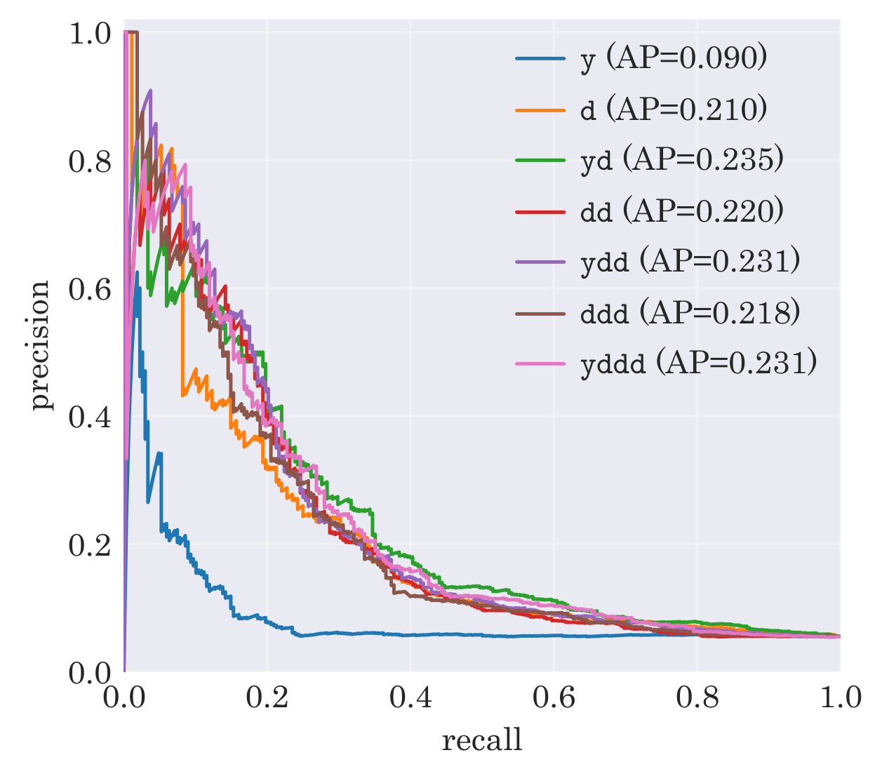
Appendix B. Pre- and Post-Candidate False-Alert Diagnostics
The main operating-rule analysis in Section 4.1, the comparator-method analysis in Section 4.2, and the feature-set sensitivity analysis in Appendix A report false-alert burden over all retained non-candidate cow-days. This pooled burden measure is appropriate for reproducible model comparison, but the retained non-candidate set includes days both before and after the calving candidate window. These two subsets have different operational interpretations: pre-candidate false alerts represent prospective inspection burden before calving, whereas post-candidate alerts may partly reflect residual behavioral disturbance after parturition.
Therefore, we provide a secondary diagnostic that separates the retained non-candidate false-alert rate into pre-candidate and post-candidate components. This split is not used for model or threshold selection. Let denote the relative day from the recorded DoB for cow i. For the default calving candidate window , let
denote the retained non-candidate cow-days before and after the candidate window, respectively. For , we compute the corresponding pre- and post-candidate false-alert rates as
where denotes a positive output under the evaluated threshold or operating rule. The pooled retained non-candidate false-alert rate used in Table 2, Table 3, and Table A1 is obtained by replacing with in the same expression. In the retained analysis set, , , and . Table A2 reports this diagnostic split for all evaluated weak-MLP feature representations and operating rules, and Table A3 reports the corresponding split for the primary weakly supervised MLP and the considered comparator methods.
Table A2.
Pre- and post-candidate false-alert diagnostics for all evaluated weak-MLP feature representations and operating rules. The base-threshold rule applies the fold-selected threshold directly to the raw daily-risk score. Rates are day-level percentages over retained non-candidate cow-days. The denominators are 1,232 pre-candidate cow-days, 3,391 post-candidate cow-days, and 4,623 retained non-candidate cow-days for all rows. This split is diagnostic only and is not used for model or threshold selection.
Table A2.
Pre- and post-candidate false-alert diagnostics for all evaluated weak-MLP feature representations and operating rules. The base-threshold rule applies the fold-selected threshold directly to the raw daily-risk score. Rates are day-level percentages over retained non-candidate cow-days. The denominators are 1,232 pre-candidate cow-days, 3,391 post-candidate cow-days, and 4,623 retained non-candidate cow-days for all rows. This split is diagnostic only and is not used for model or threshold selection.
| Feature set | Rule | (%) | (%) | (%) |
|---|---|---|---|---|
| y | Base threshold | 3.25 | 6.78 | 5.84 |
| y | Balanced rising | 2.76 | 4.45 | 4.00 |
| y | Quiet-3 | 1.38 | 2.12 | 1.93 |
| y | Triage Alert | 0.08 | 0.03 | 0.04 |
| d | Base threshold | 2.52 | 6.05 | 5.10 |
| d | Balanced rising | 2.19 | 4.84 | 4.13 |
| d | Quiet-3 | 1.62 | 3.21 | 2.79 |
| d | Triage Alert | 0.89 | 2.09 | 1.77 |
| yd | Base threshold | 1.46 | 2.62 | 2.31 |
| yd | Balanced rising | 1.46 | 2.01 | 1.86 |
| yd | Quiet-3 | 1.30 | 1.47 | 1.43 |
| yd | Triage Alert | 0.49 | 0.83 | 0.74 |
| dd | Base threshold | 2.60 | 1.86 | 2.05 |
| dd | Balanced rising | 2.60 | 1.86 | 2.05 |
| dd | Quiet-3 | 2.44 | 1.68 | 1.88 |
| dd | Triage Alert | 0.81 | 0.56 | 0.63 |
| ydd | Base threshold | 4.14 | 2.51 | 2.94 |
| ydd | Balanced rising | 4.06 | 2.51 | 2.92 |
| ydd | Quiet-3 | 3.90 | 2.06 | 2.55 |
| ydd | Triage Alert | 1.87 | 0.97 | 1.21 |
| ddd | Base threshold | 3.65 | 3.18 | 3.31 |
| ddd | Balanced rising | 3.49 | 3.18 | 3.27 |
| ddd | Quiet-3 | 3.25 | 2.60 | 2.77 |
| ddd | Triage Alert | 1.79 | 1.30 | 1.43 |
| yddd | Base threshold | 2.19 | 1.92 | 1.99 |
| yddd | Balanced rising | 2.19 | 1.89 | 1.97 |
| yddd | Quiet-3 | 2.11 | 1.62 | 1.75 |
| yddd | Triage Alert | 1.14 | 0.65 | 0.78 |
Table A3.
Pre- and post-candidate false-alert diagnostics for the primary weak exactly-one MLP and comparator methods. Rates are day-level percentages over retained non-candidate cow-days. The denominators are fixed across rows: 1,232 pre-candidate cow-days, 3,391 post-candidate cow-days, and 4,623 retained non-candidate cow-days. This split is diagnostic only and is not used for model or threshold selection.
Table A3.
Pre- and post-candidate false-alert diagnostics for the primary weak exactly-one MLP and comparator methods. Rates are day-level percentages over retained non-candidate cow-days. The denominators are fixed across rows: 1,232 pre-candidate cow-days, 3,391 post-candidate cow-days, and 4,623 retained non-candidate cow-days. This split is diagnostic only and is not used for model or threshold selection.
| Method | (%) | (%) | (%) |
|---|---|---|---|
| Weak exactly-one MLP | 4.14 | 2.51 | 2.94 |
| Weak at-least-one MLP | 4.46 | 2.68 | 3.16 |
| Weak exactly-one logistic regression | 2.11 | 2.30 | 2.25 |
| Positive-bag logistic regression | 6.74 | 5.10 | 5.54 |
| Positive-bag random forest | 6.33 | 4.63 | 5.08 |
| Positive-bag XGBoost | 4.14 | 4.36 | 4.30 |
| Rumination-drop rule | 2.52 | 6.25 | 5.26 |
| Peri-calving directional rule | 4.22 | 12.12 | 10.02 |
| Maximum absolute current-deviation rule | 5.36 | 15.48 | 12.78 |
For the primary ydd representation, Table A2 shows that the hard Alert rule produces lower day-level false-alert rates after the candidate window than before it. The base-threshold output shows the same direction, with a higher pre-candidate than post-candidate false-alert rate. Across feature sets, the diagnostic split does not change the main conclusion that stricter operating rules substantially reduce off-window burden.
In Table A3, the rule-based baselines show noticeably higher post-candidate false-alert rates, whereas the weak learned models and positive-bag classifiers show more balanced pre- and post-candidate false-alert burden. This pattern suggests that simple deviation rules are more susceptible to broader post-parturition behavioral disturbance, while learned models are less dominated by this post-candidate response. The weak exactly-one and at-least-one MLPs both have higher pre-candidate than post-candidate false-alert rates, indicating that their pooled burden is not driven primarily by post-candidate firing. Overall, the pre/post split is diagnostic rather than decisive: it clarifies where false alerts occur relative to the candidate window, while the primary burden measure remains the pooled retained non-candidate false-alert rate used in the main comparisons.
Appendix C. Triage-Policy Sensitivity
We next examine sensitivity to the operating policy used to map the learned daily-risk score to Watch and Alert triage states. In these analyses, we vary the default triage multipliers after the raw daily-risk scores have been generated. Table A4 reports results for different values of the Alert multiplier while holding the Watch multiplier fixed at , whereas Table A5 reports results for different values of the Watch multiplier while holding the Alert multiplier fixed at . The default Alert-multiplier results correspond to the hard Alert state reported in Table 2. In contrast, the default Watch-multiplier results correspond to the combined lower-confidence Watch-or-Alert stream, so they are not expected to match the hard Alert results.
To keep these policy-sensitivity summaries comparable with the results in Table 2, we report the values of the same core threshold-dependent performance measures: precision, recall, F1, MCC, candidate-window detection, false-alert or false-positive rate, and cow-level exposure. Because these sweeps vary only the operating multipliers applied to the same underlying daily-risk score, threshold-free AUPRC is unchanged and is reported once for the raw score in Table 2. The sweeps characterize the trade-off between candidate-window coverage, early warning, and false-alert burden around the default policy. They are not intended to define or optimize a farm-specific cost function. Cow-level exposure columns report proportions of cows, and false-alert or false-positive rates are computed over retained non-candidate cow-days.
Table A4.
Sensitivity of the hard Alert state to the Alert multiplier, with the Watch multiplier fixed at . Candidate-window detection is the proportion of calving cows with at least one Alert in . False-alert rate denotes the proportion of retained non-candidate cow-days with an Alert. The final column reports the proportion of cows with at least one Alert across their retained scored records.
Table A4.
Sensitivity of the hard Alert state to the Alert multiplier, with the Watch multiplier fixed at . Candidate-window detection is the proportion of calving cows with at least one Alert in . False-alert rate denotes the proportion of retained non-candidate cow-days with an Alert. The final column reports the proportion of cows with at least one Alert across their retained scored records.
|
Alert multiplier |
Precision | Recall | F1 | MCC | Detection in |
False-alert rate |
Cows with Alert |
|---|---|---|---|---|---|---|---|
| 1.0 | 0.314 | 0.201 | 0.245 | 0.217 | 0.403 | 0.0255 | 0.813 |
| 1.1 | 0.397 | 0.201 | 0.267 | 0.254 | 0.403 | 0.0177 | 0.731 |
| 1.2 | 0.481 | 0.194 | 0.277 | 0.282 | 0.388 | 0.0121 | 0.649 |
| 1.3 | 0.481 | 0.138 | 0.214 | 0.237 | 0.276 | 0.0087 | 0.470 |
| 1.4 | 0.569 | 0.108 | 0.182 | 0.232 | 0.216 | 0.0048 | 0.358 |
Table A5.
Sensitivity of the combined Watch-or-Alert positive stream to the Watch multiplier, with the Alert multiplier fixed at . Precision, recall, F1, MCC, candidate-window detection, and false-positive rate refer to the combined positive stream. Candidate-window detection is the proportion of calving cows with at least one Watch-or-Alert output in . False-positive rate denotes the proportion of retained non-candidate cow-days with a Watch-or-Alert output. The final column reports the proportion of cows with at least one Watch-only output across their retained scored records, excluding hard Alert days.
Table A5.
Sensitivity of the combined Watch-or-Alert positive stream to the Watch multiplier, with the Alert multiplier fixed at . Precision, recall, F1, MCC, candidate-window detection, and false-positive rate refer to the combined positive stream. Candidate-window detection is the proportion of calving cows with at least one Watch-or-Alert output in . False-positive rate denotes the proportion of retained non-candidate cow-days with a Watch-or-Alert output. The final column reports the proportion of cows with at least one Watch-only output across their retained scored records, excluding hard Alert days.
|
Watch multiplier |
Precision | Recall | F1 | MCC | Detection in |
False-positive rate |
Cows with Watch-only |
|---|---|---|---|---|---|---|---|
| 0.8 | 0.241 | 0.287 | 0.262 | 0.216 | 0.552 | 0.0526 | 0.754 |
| 0.9 | 0.271 | 0.261 | 0.266 | 0.225 | 0.507 | 0.0407 | 0.619 |
| 1.0 | 0.322 | 0.239 | 0.274 | 0.241 | 0.463 | 0.0292 | 0.470 |
The Alert-multiplier sweep in Table A4 illustrates the expected burden–sensitivity trade-off: stricter Alert thresholds reduce the false-alert rate and generally increase precision, but they also reduce recall and candidate-window detection. The Watch-multiplier sweep in Table A5 shows that the lower-confidence combined Watch-or-Alert stream can be made more or less permissive without changing the underlying daily-risk score. Together, these findings reinforce the main-text recommendation that deployment should expose the raw risk score and allow users to adjust the triage policy according to local inspection capacity and risk tolerance.
Appendix D. Comparator-Method Fold-Level Summaries
Table A6 reports fold-level mean ± standard deviation performance summaries for the primary weak exactly-one MLP and the comparator methods in Table 3. These summaries are computed across the four held-out outer folds and are intended to describe fold-to-fold variation rather than to support formal significance claims from our relatively small dataset. In Table 3, we pool held-out predictions before computing each performance measure. In Table A6, we compute the same performance measures separately within each fold and then report their mean and standard deviation across folds. As a result, the fold-level summaries need not exactly match the pooled values in Table 3, especially for measures that depend on fold composition, score ranking, thresholding, or cow-level aggregation. Learned methods use inner-fold hyperparameter and threshold selection, so each row represents a complete four-fold evaluation for that method.
Table A6.
Fold-level mean ± standard deviation for the primary weak exactly-one MLP and comparator methods. Performance measures are computed separately on each outer test fold and then summarized across the four folds. These summaries complement the pooled out-of-fold values in Table 3. Learned methods use inner-fold hyperparameter and threshold selection, so each row represents a complete four-fold evaluation for that method.
Table A6.
Fold-level mean ± standard deviation for the primary weak exactly-one MLP and comparator methods. Performance measures are computed separately on each outer test fold and then summarized across the four folds. These summaries complement the pooled out-of-fold values in Table 3. Learned methods use inner-fold hyperparameter and threshold selection, so each row represents a complete four-fold evaluation for that method.
| Method | Day-level measures | Operational measures | |||||
|---|---|---|---|---|---|---|---|
| Precision | Recall | F1 | MCC | AUPRC | Detection in |
False- alert rate |
|
| Weak exactly-one MLP | |||||||
| Weak at-least-one MLP | |||||||
| Weak exactly-one LR | |||||||
| Positive-bag LR | |||||||
| Positive-bag random forest | |||||||
| Positive-bag XGBoost | |||||||
| Rumination-drop rule | |||||||
| Directional peri-calving rule | |||||||
| Max-absolute-deviation rule | |||||||
Appendix E. Missingness Sensitivity: Complete-Case Modeling Without Masks
The feature-set sensitivity results in Appendix A retain all eligible cow-day records and use explicit missingness indicators for unavailable baseline-derived or lagged-history components. As a complementary sensitivity check, we repeat the feature-set ablation under a complete-case, no-mask formulation: for each feature set, we retain only records with fully available continuous components and remove the explicit missingness indicators. This complete-case setting differs from the main analysis in two important ways: it discards cow-day records with unavailable baseline-referenced or lagged-history features and changes both the retained evaluation set and the feature representation. In particular, some candidate-window cow-days are lost under this stricter requirement, so the resulting cow-level detection summaries are not directly comparable to those from the main missingness-aware analysis. The aim of this ablation is therefore not to define an alternative main model, but to assess whether the main conclusions depend materially on the missingness-aware treatment of incomplete early-history records.
Table A7.
Complete-case, no-mask missingness ablation for all feature sets. Each row uses only cow-days with fully available continuous components for the corresponding feature set, and explicit missingness indicators are removed. False-alert rate denotes the proportion of retained non-candidate cow-days with a positive output.
Table A7.
Complete-case, no-mask missingness ablation for all feature sets. Each row uses only cow-days with fully available continuous components for the corresponding feature set, and explicit missingness indicators are removed. False-alert rate denotes the proportion of retained non-candidate cow-days with a positive output.
| Feature set |
Cow-days | Candidate cow-days |
Prec. | Rec. | F1 | MCC | AUPRC | Det. in |
False-alert rate |
|---|---|---|---|---|---|---|---|---|---|
| y | 4,891 | 268 | 0.118 | 0.134 | 0.125 | 0.071 | 0.090 | 0.209 | 0.0584 |
| d | 4,489 | 248 | 0.252 | 0.226 | 0.238 | 0.197 | 0.143 | 0.381 | 0.0391 |
| yd | 4,489 | 248 | 0.272 | 0.278 | 0.275 | 0.232 | 0.228 | 0.433 | 0.0436 |
| dd | 4,355 | 236 | 0.280 | 0.246 | 0.262 | 0.223 | 0.209 | 0.425 | 0.0362 |
| ydd | 4,355 | 236 | 0.358 | 0.246 | 0.291 | 0.264 | 0.223 | 0.425 | 0.0252 |
| ddd | 4,221 | 225 | 0.293 | 0.258 | 0.274 | 0.237 | 0.248 | 0.418 | 0.0350 |
| yddd | 4,221 | 225 | 0.256 | 0.222 | 0.238 | 0.199 | 0.196 | 0.366 | 0.0363 |
As shown in Table A7, the complete-case analysis broadly supports the main conclusions. For the primary ydd representation, removing incomplete cow-day records and missingness indicators increases day-level F1 from to and MCC from to , while reducing the retained candidate-window cow-days from 268 to 236. Candidate-window detection decreases from in the main missingness-aware analysis to in the complete-case analysis, and AUPRC decreases slightly from to . Among the complete-case variants, ydd gives the strongest F1/MCC trade-off and the lowest false-alert rate among the non-raw feature sets. The yd representation gives slightly higher candidate-window detection, and ddd gives the highest AUPRC, but neither improves the overall deployment-oriented balance relative to ydd. Because the complete-case formulation discards early-history records and changes the evaluated population, we retain the all-row missingness-aware ydd formulation as the primary analysis and deployment model.
Appendix F. Candidate-Window Sensitivity
We examine sensitivity to the weak-supervision window used during model training. For each candidate-window definition, we rerun the weakly supervised MLP training and cow-grouped nested cross-validation using the primary ydd feature set, the same optimization settings, and the same hyperparameter search space. Thus, model fitting, inner-fold hyperparameter selection, and threshold selection are repeated under each candidate-window definition, rather than applying a post hoc relabeling to existing scores. The case provides the primary-window reference under the same retraining workflow.
Table A8.
Retrained candidate-window sensitivity for the weakly supervised MLP. Each row is a separate cow-grouped nested cross-validation run using the same primary feature set, optimization settings, and hyperparameter search space but a different candidate-window definition. Here, denotes the candidate-window definition used in that row, and false-alert rate denotes the proportion of retained non-candidate cow-days with a positive output.
Table A8.
Retrained candidate-window sensitivity for the weakly supervised MLP. Each row is a separate cow-grouped nested cross-validation run using the same primary feature set, optimization settings, and hyperparameter search space but a different candidate-window definition. Here, denotes the candidate-window definition used in that row, and false-alert rate denotes the proportion of retained non-candidate cow-days with a positive output.
| Candidate window |
Candidate cow-days |
Precision | Recall | F1 | MCC | AUPRC | Detection in |
False-alert rate |
|---|---|---|---|---|---|---|---|---|
| 398 | 0.265 | 0.229 | 0.245 | 0.184 | 0.224 | 0.619 | 0.0563 | |
| 268 | 0.323 | 0.243 | 0.277 | 0.244 | 0.231 | 0.470 | 0.0294 | |
| 402 | 0.294 | 0.259 | 0.275 | 0.215 | 0.225 | 0.649 | 0.0557 | |
| 532 | 0.250 | 0.244 | 0.247 | 0.156 | 0.225 | 0.716 | 0.0895 |
Table A8 shows that broader candidate windows increase cow-level candidate-window detection, but they do not improve the deployment-oriented operating trade-off. The pre-calving window increases detection to , but reduces F1 and MCC to and , respectively, and increases the false-alert rate to . The window gives the closest F1 to the primary window ( versus ) and the highest recall among the four settings, but its MCC is lower () and its false-alert rate is almost twice as high ( versus ). The widest window, , gives the highest candidate-window detection (), but has the weakest MCC () and the highest false-alert rate ().
Overall, these results support as the primary candidate-window convention for the daily triage setting. Wider windows make cow-level detection easier by construction and can recover more animals within the expanded event window, but they also shift the model toward lower thresholds and higher off-window burden. The primary window therefore provides the cleaner operating compromise among the evaluated definitions.
Appendix G. Deployment Computational and Memory Complexity
We consider deployment of the final model using the primary feature representation in Eq. (1). The deployed model uses a single hidden layer with width , determined by the automatic hidden-width rule , where is the number of continuous non-mask input features. For the primary representation, , giving . Excluding upstream behavior classification and daily 06:00–06:00 aggregation, the online scoring and triage procedure is lightweight in both computation and memory.
Let denote the number of behavior channels and the causal baseline window. Once the daily behavior summary is available, feature construction requires the baseline-referenced deviation vector , the previous-retained-day deviation vector , the history-gap variable , and the associated missingness indicators. In the primary representation, the continuous part contains 16 values: five raw behavior summaries, five current deviations, five previous-retained-day deviations, and one history-gap variable. The processed model input consists of these 16 continuous values plus 11 missingness indicators for the baseline-derived, lagged, and history-gap components, giving a full input dimension of .
A direct implementation of the causal baseline calculation scans at most stored daily behavior values per cow-day before applying the robust baseline rule. If the robust summary is implemented by sorting, this requires at most five short sorts, each over a window of length no greater than 14, followed by five trimmed-mean calculations. The remaining feature-construction operations are also small: five current-deviation calculations, five previous-retained-day deviation lookups, one history-gap update, and 11 missingness-flag assignments. Rolling maintenance of the baseline statistics could reduce the fixed-window scan further, but even the direct implementation is negligible at this scale.
The deployed scoring model is a one-hidden-layer multilayer perceptron. With processed inputs and hidden units, the hidden layer uses input–hidden weights and 9 hidden biases. The output layer uses 9 hidden–output weights and one output bias. Therefore, the total number of trainable parameters is .
A single forward pass requires 243 input–hidden multiplications, 243 corresponding additions or bias accumulations, 9 nonlinear activations, 9 hidden–output multiplications, 9 corresponding additions or bias accumulations, and one final sigmoid transformation. Thus, scoring one cow-day requires only 252 multiplications, approximately 252 additions, 9 hidden activations, and one sigmoid evaluation.
The runtime memory requirement is also modest. For each cow, a direct implementation needs the most recent daily summaries for behavior classes, corresponding to 70 scalar behavior values. It also stores the previous deviation vector of length 5, the previous scored-day risk score for the balanced-rising rule, and a few Boolean or integer state variables for the quiet-window rule and missingness bookkeeping. Even using 64-bit floating point values, the core numeric state is well below 1 kB per cow before ordinary software-container overhead. The model itself stores only 262 parameters, corresponding to about 1 kB in 32-bit floating point or about 2 kB in 64-bit floating point.
The practical operational outputs are the raw daily risk score and the resulting triage state. The base-threshold, balanced-rising, and quiet-window flags are useful diagnostic intermediates, but they do not need to be exposed as separate end-user outputs.
References
- Kang, J.; Weik, F.; Sanderson, N.; Robertson, D.; Archer, J.A. Using foetal age estimates to substitute birth date recording in beef cattle evaluations. Proceedings of the Proceedings of the Association for the Advancement of Animal Breeding and Genetics 2023, Vol. 25, 126–129. [Google Scholar]
- Dematawewa, C.M.B.; Berger, P.J. Effect of dystocia on yield, fertility, and cow losses and an economic evaluation of dystocia scores for Holsteins. J. Dairy Sci. 1997, 80, 754–761. [Google Scholar] [CrossRef] [PubMed]
- Lombard, J.E.; Garry, F.B.; Tomlinson, S.M.; Garber, L.P. Impacts of dystocia on health and survival of dairy calves. J. Dairy Sci. 2007, 90, 1751–1760. [Google Scholar] [CrossRef] [PubMed]
- Saint-Dizier, M.; Chastant-Maillard, S. Methods and on-farm devices to predict calving time in cattle. Vet. J. 2015, 205, 349–356. [Google Scholar] [CrossRef] [PubMed]
- Szenci, O. Accuracy to predict the onset of calving in dairy farms by using different precision livestock farming devices. Animals 2022, 12, 2006. [Google Scholar] [CrossRef] [PubMed]
- Crociati, M.; Sylla, L.; De Vincenzi, A.; Stradaioli, G.; Monaci, M. How to predict parturition in cattle? A literature review of automatic devices and technologies for remote monitoring and calving prediction. Animals 2022, 12, 405. [Google Scholar] [CrossRef] [PubMed]
- Rutten, C.J.; Kamphuis, C.; Hogeveen, H.; Huijps, K.; Nielen, M.; Steeneveld, W. Sensor data on cow activity, rumination, and ear temperature improve prediction of the start of calving in dairy cows. Comput. Electron. Agric. 2017, 132, 108–118. [Google Scholar] [CrossRef]
- Krieger, S.; Oczak, M.; Lidauer, L.; Berger, A.; Kickinger, F.; Öhlschuster, M.; Auer, W.; Drillich, M.; Iwersen, M. An ear-attached accelerometer as an on-farm device to predict the onset of calving in dairy cows. Biosyst. Eng. 2019, 184, 190–199. [Google Scholar] [CrossRef]
- Miller, G.A.; Mitchell, M.; Barker, Z.E.; Giebel, K.; Codling, E.A.; Amory, J.R.; Michie, C.; Davison, C.; Tachtatzis, C.; Andonovic, I.; et al. Using animal-mounted sensor technology and machine learning to predict time-to-calving in beef and dairy cows. Animal 2020, 14, 1304–1312. [Google Scholar] [CrossRef] [PubMed]
- Keceli, A.S.; Catal, C.; Kaya, A.; Tekinerdogan, B. Development of a recurrent neural networks-based calving prediction model using activity and behavioral data. Comput. Electron. Agric. 2020, 170, 105285. [Google Scholar] [CrossRef]
- Liseune, A.; Van den Poel, D.; Hut, P.R.; van Eerdenburg, F.J.C.M.; Hostens, M. Leveraging sequential information from multivariate behavioral sensor data to predict the moment of calving in dairy cattle using deep learning. Comput. Electron. Agric. 2021, 191, 106566. [Google Scholar] [CrossRef]
- Vázquez-Diosdado, J.A.; Gruhier, J.; Miguel-Pacheco, G.G.; Green, M.; Dottorini, T.; Kaler, J. Accurate prediction of calving in dairy cows by applying feature engineering and machine learning. Prev. Vet. Med. 2023, 219, 106007. [Google Scholar] [CrossRef] [PubMed]
- Yang, L.; Zhao, J.; Ying, X.; Lu, C.; Zhou, X.; Gao, Y.; Wang, L.; Liu, H.; Song, H. Utilization of deep learning models to predict calving time in dairy cattle from tail acceleration data. Comput. Electron. Agric. 2024, 225, 109253. [Google Scholar] [CrossRef]
- Benaissa, S.; Tuyttens, F.A.M.; Plets, D.; Trogh, J.; Martens, L.; Vandaele, L.; Joseph, W.; Sonck, B. Calving and estrus detection in dairy cattle using a combination of indoor localization and accelerometer sensors. Comput. Electron. Agric. 2020, 168, 105153. [Google Scholar] [CrossRef]
- Giaretta, E.; Marliani, G.; Postiglione, G.; Magazzù, G.; Pantò, F.; Mari, G.; Formigoni, A.; Accorsi, P.A.; Mordenti, A. Calving time identified by the automatic detection of tail movements and rumination time, and observation of cow behavioural changes. Animal 2021, 15, 100071. [Google Scholar] [CrossRef] [PubMed]
- Schirmann, K.; Chapinal, N.; Weary, D.M.; Vickers, L.; von Keyserlingk, M.A.G. Short communication: Rumination and feeding behavior before and after calving in dairy cows. J. Dairy Sci. 2013, 96, 7088–7092. [Google Scholar] [CrossRef] [PubMed]
- Chang, A.Z.; Fogarty, E.S.; Swain, D.L.; García-Guerra, A.; Trotter, M.G. Accelerometer derived rumination monitoring detects changes in behaviour around parturition. Appl. Anim. Behav. Sci. 2022, 247, 105566. [Google Scholar] [CrossRef]
- Smith, D.; McNally, J.; Little, B.; Ingham, A.; Schmoelzl, S. Automatic detection of parturition in pregnant ewes using a three-axis accelerometer. Comput. Electron. Agric. 2020, 173, 105392. [Google Scholar] [CrossRef]
- Turner, K.E.; Sohel, F.; Harris, I.; Ferguson, M.; Thompson, A. Lambing event detection using deep learning from accelerometer data. Comput. Electron. Agric. 2023, 208, 107787. [Google Scholar] [CrossRef]
- Gonçalves, P.; Marques, M.R.; Nyamuryekung’e, S.; Jorgensen, G.H.M. Small ruminant parturition detection based on inertial sensors—A review. Animals 2024, 14, 2885. [Google Scholar] [CrossRef] [PubMed]
- Ferreira, J.; Gonçalves, P.; Antunes, M. A two-stage approach for lambing detection. Smart Agric. Technol. 2025, 12, 101438. [Google Scholar] [CrossRef]
- Ramos, H.; Gonçalves, P.; Corujo, D.; Antunes, M. A machine learning-based wearable system for automated detection of sheep parturition events using accelerometer data. Comput. Electron. Agric. 2026, 248, 111784. [Google Scholar] [CrossRef]
- García García, M.J.; Maroto Molina, F.; Pérez Marín, C.C.; Pérez Marín, D.C. Potential for automatic detection of calving in beef cows grazing on rangelands from Global Navigate Satellite System collar data. Animal 2023, 17, 100901. [Google Scholar] [CrossRef] [PubMed]
- Wang, Y.; Perea, A.; Cao, H.; Bakir, M.; Utsumi, S. A two-stage machine learning approach for calving detection in rangeland cattle. Agriculture 2025, 15, 1434. [Google Scholar] [CrossRef]
- Ilse, M.; Tomczak, J.M.; Welling, M. Attention-based deep multiple instance learning. Proc. Proc. 35th Int. Conf. Mach. Learn. PMLR 2018, Vol. 80, Proceedings of Machine Learning Research, 2127–2136. [Google Scholar]
- Riaboff, L.; Shalloo, L.; Smeaton, A.F.; Couvreur, S.; Madouasse, A.; Keane, M.T. Predicting livestock behaviour using accelerometers: A systematic review of processing techniques for ruminant behaviour prediction from raw accelerometer data. Comput. Electron. Agric. 2022, 192, 106610. [Google Scholar] [CrossRef]
- Wang, L.; Arablouei, R.; Alvarenga, F.A.; Bishop-Hurley, G.J. Classifying animal behavior from accelerometry data via recurrent neural networks. Comput. Electron. Agric. 2023, 206, 107647. [Google Scholar] [CrossRef]
- Arablouei, R.; Bishop-Hurley, G.J.; Bagnall, N.; Ingham, A. Cattle behavior recognition from accelerometer data: Leveraging in-situ cross-device model learning. Comput. Electron. Agric. 2024, 227, 109546. [Google Scholar] [CrossRef]
- Chang, A.Z.; Fogarty, E.S.; Moraes, L.E.; García-Guerra, A.; Swain, D.L.; Trotter, M.G. Detection of rumination in cattle using an accelerometer ear-tag: A comparison of analytical methods and individual animal and generic models. Comput. Electron. Agric. 2022, 192, 106595. [Google Scholar] [CrossRef]
- Arablouei, R.; Wang, L.; Phillips, C.; Currie, L.; Yates, J.; Bishop-Hurley, G. In-situ animal behavior classification using knowledge distillation and fixed-point quantization. Smart Agric. Technol. 2023, 4, 100159. [Google Scholar] [CrossRef]
- Eckhardt, R.; Arablouei, R.; Ingham, A.; McCosker, K.; Bernhardt, H. Livestock behaviour forecasting via generative artificial intelligence. Smart Agric. Technol. 2025, 11, 100987. [Google Scholar] [CrossRef]
- Arablouei, R.; Do, B.; Bagnall, N.; McNally, J.; Bishop-Hurley, G.; Ingham, A. Lightweight on-animal behavior classification and estrus detection in grazing cattle via ear-tag accelerometers. Smart Agric. Technol. 2026, 13, 101851. [Google Scholar] [CrossRef]
- Kingma, D.P.; Ba, J. Adam: A method for stochastic optimization. In Proceedings of the International Conference on Learning Representations (ICLR), 2015. [Google Scholar]
Figure 1.
Representative grazing cattle from the field setting used for the main calving study. The study uses daily behavior summaries derived from ear-tag accelerometers to evaluate day-level calving-oriented monitoring under practical grazing-system conditions.
Figure 1.
Representative grazing cattle from the field setting used for the main calving study. The study uses daily behavior summaries derived from ear-tag accelerometers to evaluate day-level calving-oriented monitoring under practical grazing-system conditions.
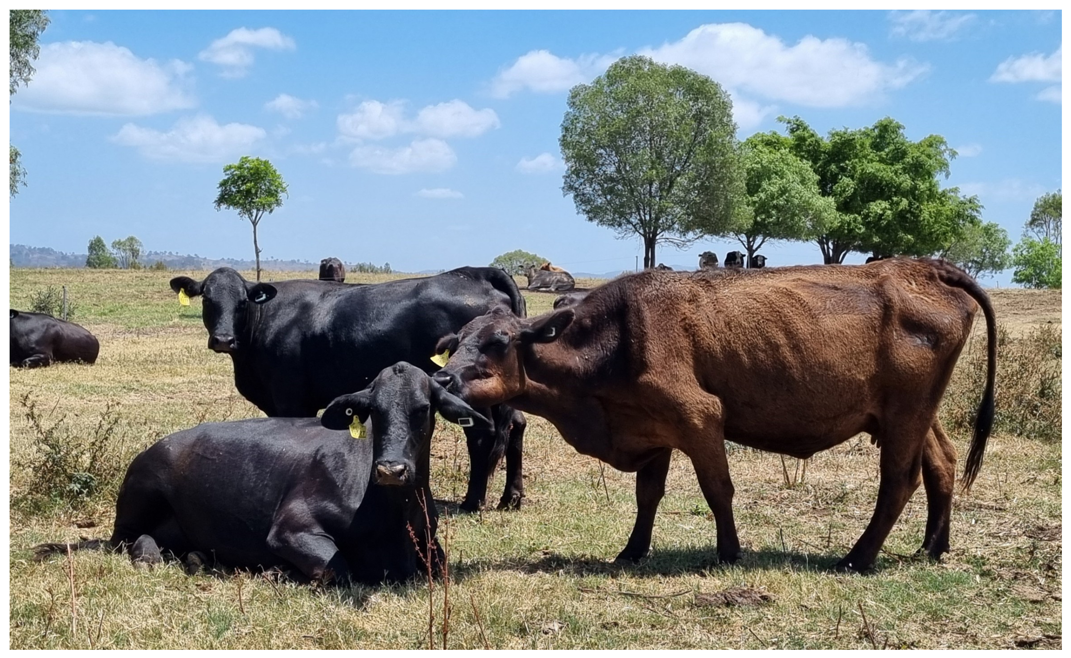
Figure 2.
Schematic of the daily candidate-window formulation. The pipeline aggregates behavior predictions into fixed 06:00–06:00 days, while the field annotation records only the DoB. Thus, the weakly supervised model treats the positive day as latent within the two-day candidate set , rather than assigning the label to a single observed day by assumption.
Figure 2.
Schematic of the daily candidate-window formulation. The pipeline aggregates behavior predictions into fixed 06:00–06:00 days, while the field annotation records only the DoB. Thus, the weakly supervised model treats the positive day as latent within the two-day candidate set , rather than assigning the label to a single observed day by assumption.
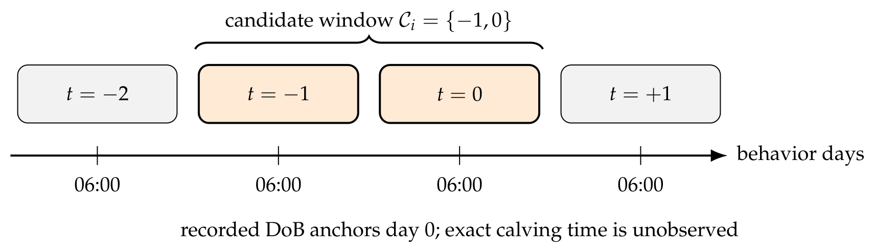
Figure 3.
Overview of the proposed strictly causal calving-oriented monitoring framework. The pipeline converts ear-tag accelerometer readings into daily behavior summaries, constructs causal behavior-history features, scores each cow-day with a weakly supervised daily-risk model, and maps the resulting score to Low, Watch, and Alert triage states.
Figure 3.
Overview of the proposed strictly causal calving-oriented monitoring framework. The pipeline converts ear-tag accelerometer readings into daily behavior summaries, constructs causal behavior-history features, scores each cow-day with a weakly supervised daily-risk model, and maps the resulting score to Low, Watch, and Alert triage states.
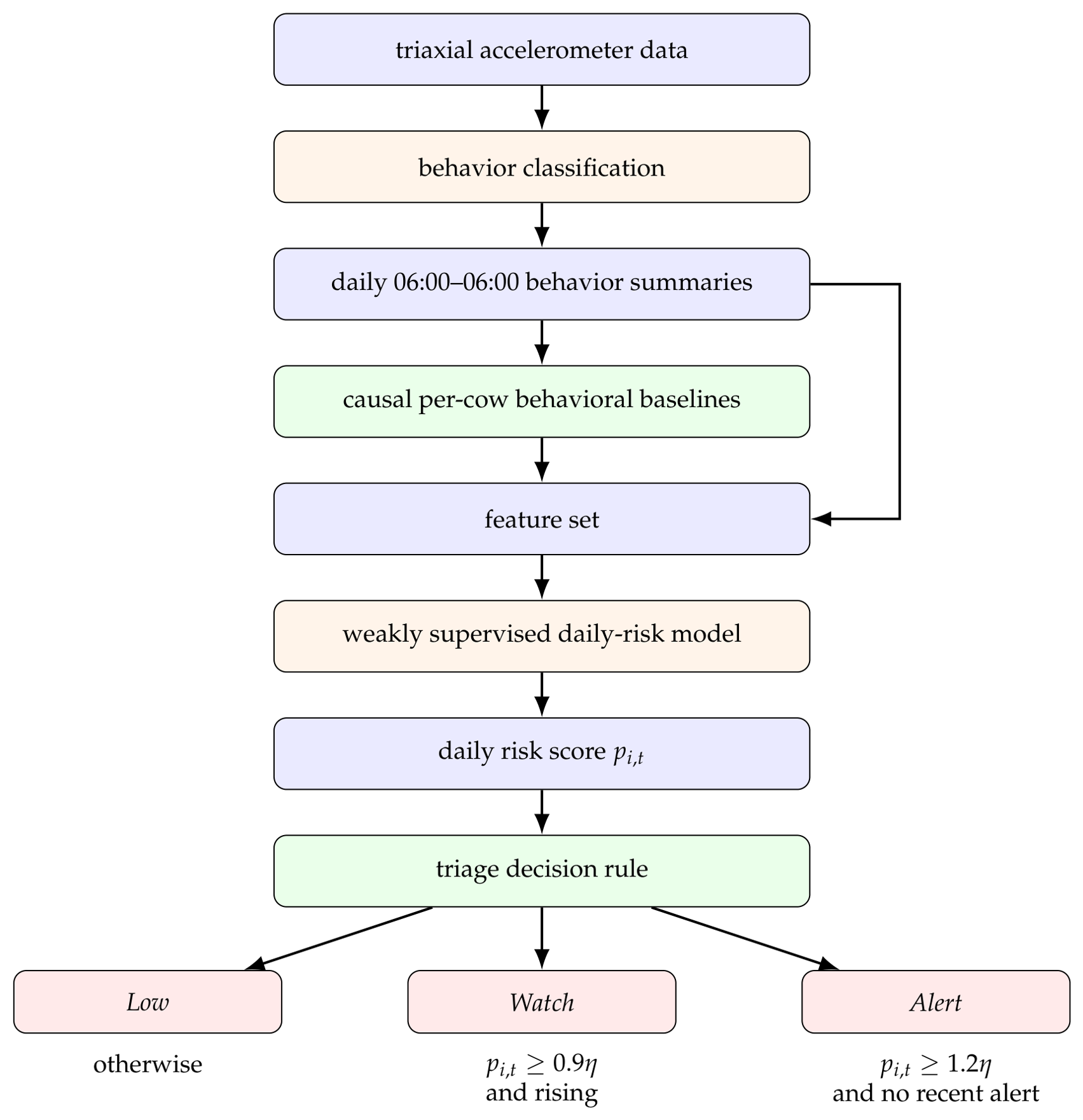
Figure 4.
Illustration of the causal hybrid baseline for one cow and one behavior class b. The baseline for day t uses only available historical values from the window , and the deviation feature is defined as the current daily value minus this cow-specific baseline.
Figure 4.
Illustration of the causal hybrid baseline for one cow and one behavior class b. The baseline for day t uses only available historical values from the window , and the deviation feature is defined as the current daily value minus this cow-specific baseline.
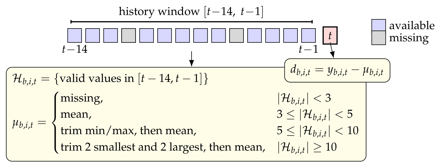
Figure 5.
Descriptive event-aligned summaries of baseline-referenced daily behavior deviations for the five behavior classes used in this study. Bars show medians and error bars show interquartile ranges across cows with available data at each relative day. The shaded vertical band marks the candidate window relative to the recorded DoB. This retrospective visualization motivates the deviation-from-baseline feature design but is not used as an online model input.
Figure 5.
Descriptive event-aligned summaries of baseline-referenced daily behavior deviations for the five behavior classes used in this study. Bars show medians and error bars show interquartile ranges across cows with available data at each relative day. The shaded vertical band marks the candidate window relative to the recorded DoB. This retrospective visualization motivates the deviation-from-baseline feature design but is not used as an online model input.
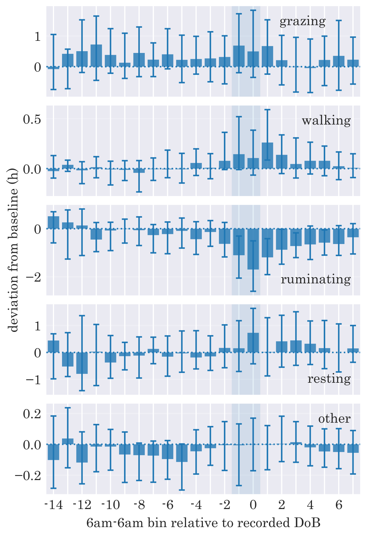
Figure 6.
Precision–recall curve for pooled out-of-fold raw daily-risk scores from the primary weakly supervised MLP. The curve is computed by sweeping a single threshold over the pooled raw scores and provides a threshold-free view of the precision–recall trade-off under strong day-level class imbalance. The markers show the evaluated operating points: the fold-selected base-threshold output used for the raw-score row in Table 2 and the stricter hard Alert output used in the triage policy. Because these operating points use fold-specific selected thresholds, and the hard Alert point also includes the deployment triage rule, the markers are not constrained to lie exactly on the pooled single-threshold PR curve.
Figure 6.
Precision–recall curve for pooled out-of-fold raw daily-risk scores from the primary weakly supervised MLP. The curve is computed by sweeping a single threshold over the pooled raw scores and provides a threshold-free view of the precision–recall trade-off under strong day-level class imbalance. The markers show the evaluated operating points: the fold-selected base-threshold output used for the raw-score row in Table 2 and the stricter hard Alert output used in the triage policy. Because these operating points use fold-specific selected thresholds, and the hard Alert point also includes the deployment triage rule, the markers are not constrained to lie exactly on the pooled single-threshold PR curve.
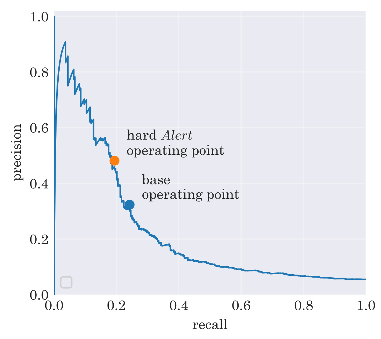
Figure 7.
Event-aligned heatmap of pooled out-of-fold raw daily-risk scores from the primary weakly supervised MLP. Each row corresponds to one cow and each column to a 06:00–06:00 behavioral day relative to the recorded DoB. Cows are ranked by their maximum score over the candidate window . Blank cells indicate unavailable cow-day scores. The figure highlights heterogeneous peri-calving score elevations across cows.
Figure 7.
Event-aligned heatmap of pooled out-of-fold raw daily-risk scores from the primary weakly supervised MLP. Each row corresponds to one cow and each column to a 06:00–06:00 behavioral day relative to the recorded DoB. Cows are ranked by their maximum score over the candidate window . Blank cells indicate unavailable cow-day scores. The figure highlights heterogeneous peri-calving score elevations across cows.
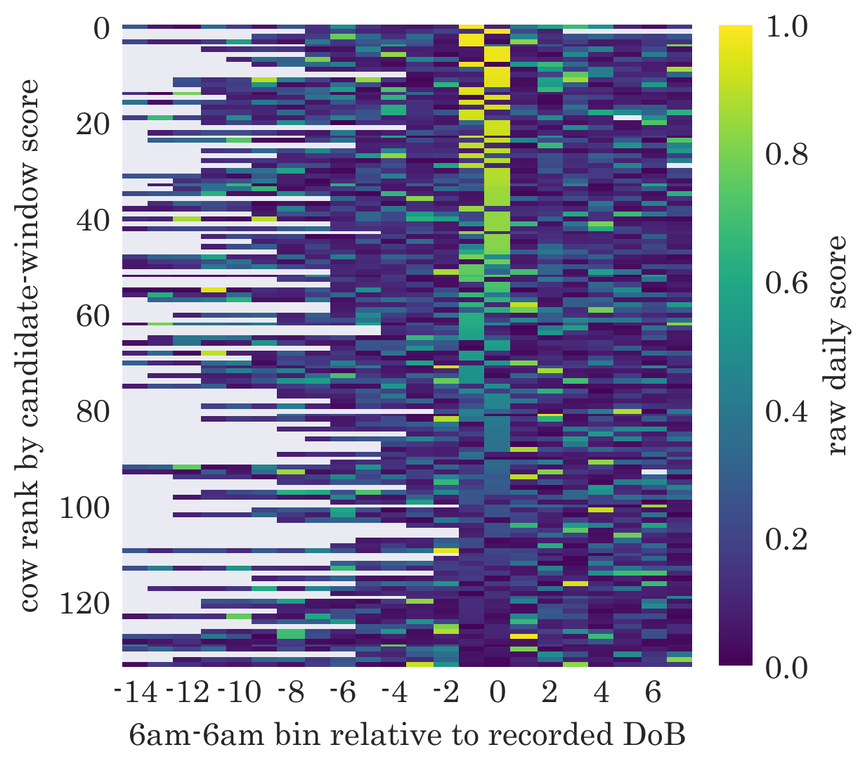
Figure 8.
Event-aligned strip plot of pooled out-of-fold raw daily-risk scores from the primary weakly supervised MLP. Points represent individual scored cow-days, aligned by 06:00–06:00 behavioral day relative to the recorded DoB. The solid line shows the median score, the translucent band shows the interquartile range, and the shaded vertical region marks the candidate window . The plot shows a modest upward shift in scores around the candidate window, with substantial overlap between candidate and surrounding non-candidate days.
Figure 8.
Event-aligned strip plot of pooled out-of-fold raw daily-risk scores from the primary weakly supervised MLP. Points represent individual scored cow-days, aligned by 06:00–06:00 behavioral day relative to the recorded DoB. The solid line shows the median score, the translucent band shows the interquartile range, and the shaded vertical region marks the candidate window . The plot shows a modest upward shift in scores around the candidate window, with substantial overlap between candidate and surrounding non-candidate days.
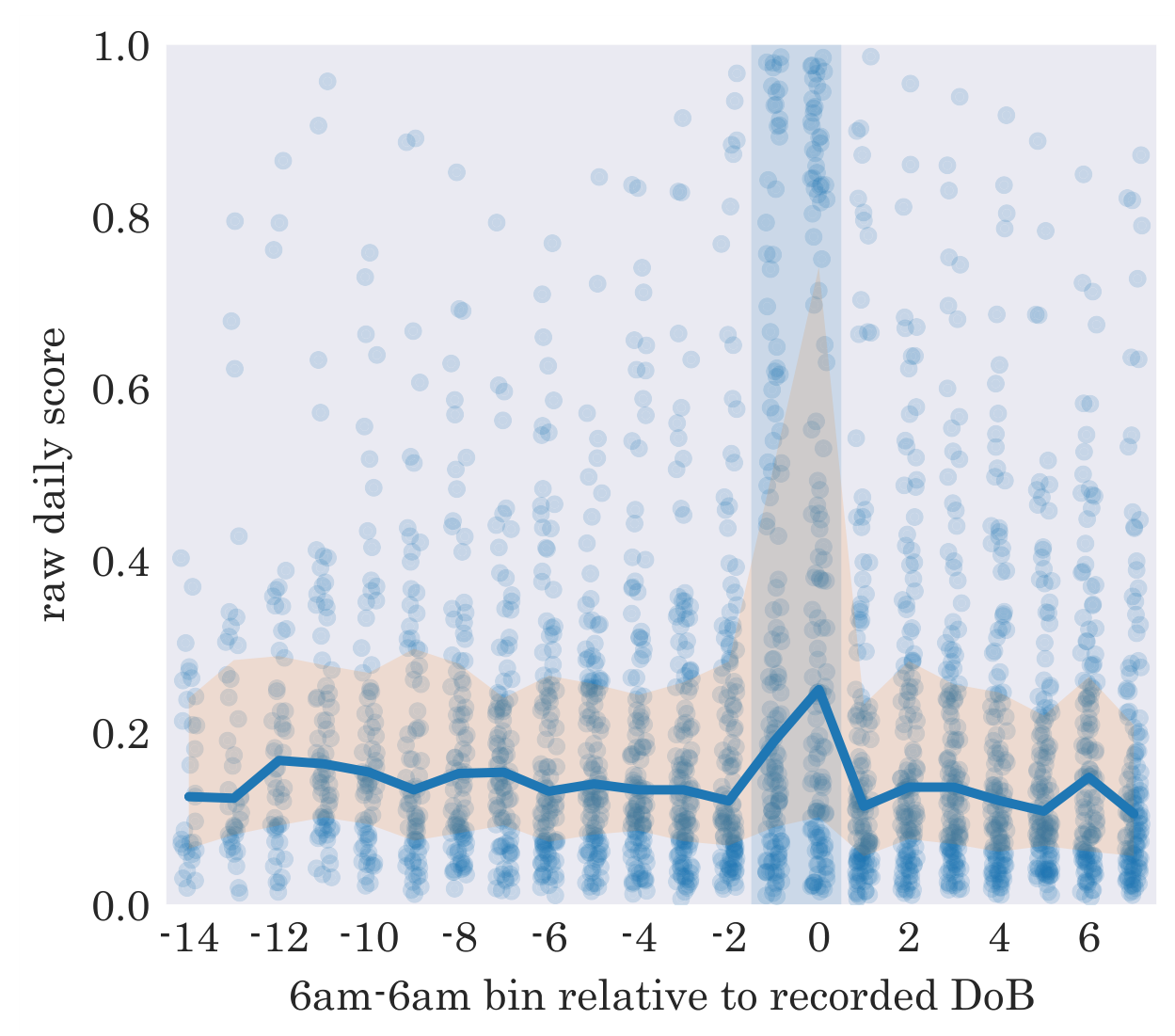
Table 1.
Key statistics for the daily behavior-summary datasets. Both datasets are represented as 06:00–06:00 cow-day records with five behavior classes: grazing, walking, ruminating, resting, and other. The independent non-calving cohort is used only for frozen-model scoring and triage-burden analysis.
Table 1.
Key statistics for the daily behavior-summary datasets. Both datasets are represented as 06:00–06:00 cow-day records with five behavior classes: grazing, walking, ruminating, resting, and other. The independent non-calving cohort is used only for frozen-model scoring and triage-burden analysis.
| Main calving study | Independent non-calving cohort | |
|---|---|---|
| behavior-day date range | 22 Oct 2025 – 30 Nov 2025 | 31 Jan 2025 – 7 May 2025 |
| cows retained for analysis | 134 | 31 |
| scored cow-days | 4,891 | 1,547 |
| mean analyzed days per cow | 36.5 | 49.9 |
| calving candidate-window cow-days | 268 | — |
| non-candidate cow-days retained | 4,623 | — |
| cow-days with complete primary features | 4,355 | — |
| cow-days with incomplete primary features | 536 | — |
Table 2.
Internal evaluation of the primary daily-risk model and the deployment-oriented operating rules derived from it. Values are computed from pooled held-out outer-fold predictions. Precision, recall, F1, and MCC are threshold-dependent day-level performance measures, whereas AUPRC summarizes the raw daily scores without thresholding. The base-threshold row applies the fold-selected threshold directly to the raw daily-risk score, whereas the operating-rule rows apply additional causal post-processing to the same score. Detection in is a cow-level candidate-window measure. False-alert rate denotes the proportion of retained non-candidate cow-days with a positive output. The triage row reports the hard Alert state only.
Table 2.
Internal evaluation of the primary daily-risk model and the deployment-oriented operating rules derived from it. Values are computed from pooled held-out outer-fold predictions. Precision, recall, F1, and MCC are threshold-dependent day-level performance measures, whereas AUPRC summarizes the raw daily scores without thresholding. The base-threshold row applies the fold-selected threshold directly to the raw daily-risk score, whereas the operating-rule rows apply additional causal post-processing to the same score. Detection in is a cow-level candidate-window measure. False-alert rate denotes the proportion of retained non-candidate cow-days with a positive output. The triage row reports the hard Alert state only.
| Operating rule | Day-level measures | Operational measures | |||||
|---|---|---|---|---|---|---|---|
| Precision | Recall | F1 | MCC | AUPRC | Detection in | False-alert rate | |
| Base threshold | 0.323 | 0.243 | 0.277 | 0.244 | 0.231 | 0.470 | 0.0294 |
| Balanced rising | 0.322 | 0.239 | 0.274 | 0.241 | — | 0.463 | 0.0292 |
| Quiet-3 | 0.314 | 0.201 | 0.245 | 0.217 | — | 0.403 | 0.0255 |
| Triage Alert | 0.481 | 0.194 | 0.277 | 0.282 | — | 0.388 | 0.0121 |
Table 3.
Internal comparison of the primary weakly supervised MLP and comparator methods on the primary feature set. Values are computed from pooled held-out outer-fold predictions. For learned methods, threshold-dependent metrics are computed from thresholded raw daily-risk scores. The weak exactly-one logistic regression (LR) uses the same exactly-one weak-supervision likelihood as the primary MLP but with a linear logistic score. The weak at-least-one MLP uses the same one-hidden-layer architecture class as the primary MLP but replaces the exactly-one candidate-window likelihood with an at-least-one likelihood. The positive-bag LR, random forest, and XGBoost methods are supervised comparators that treat both candidate-window days as positive. Rule methods use causal deviation-derived scores with thresholds selected using the same inner-validation structure. Detection in is cow-level candidate-window detection.
Table 3.
Internal comparison of the primary weakly supervised MLP and comparator methods on the primary feature set. Values are computed from pooled held-out outer-fold predictions. For learned methods, threshold-dependent metrics are computed from thresholded raw daily-risk scores. The weak exactly-one logistic regression (LR) uses the same exactly-one weak-supervision likelihood as the primary MLP but with a linear logistic score. The weak at-least-one MLP uses the same one-hidden-layer architecture class as the primary MLP but replaces the exactly-one candidate-window likelihood with an at-least-one likelihood. The positive-bag LR, random forest, and XGBoost methods are supervised comparators that treat both candidate-window days as positive. Rule methods use causal deviation-derived scores with thresholds selected using the same inner-validation structure. Detection in is cow-level candidate-window detection.
| Method | Day-level measures | Operational measures | |||||
|---|---|---|---|---|---|---|---|
| Precision | Recall | F1 | MCC | AUPRC | Detection in |
False- alert rate |
|
| Weak exactly-one MLP | 0.323 | 0.243 | 0.277 | 0.244 | 0.231 | 0.470 | 0.0294 |
| Weak at-least-one MLP | 0.324 | 0.261 | 0.289 | 0.254 | 0.252 | 0.507 | 0.0316 |
| Weak exactly-one LR | 0.358 | 0.216 | 0.270 | 0.247 | 0.204 | 0.418 | 0.0225 |
| Positive-bag LR | 0.251 | 0.321 | 0.282 | 0.237 | 0.219 | 0.470 | 0.0554 |
| Positive-bag random forest | 0.281 | 0.343 | 0.309 | 0.266 | 0.232 | 0.545 | 0.0508 |
| Positive-bag XGBoost | 0.276 | 0.284 | 0.280 | 0.238 | 0.230 | 0.470 | 0.0430 |
| Rumination-drop rule | 0.250 | 0.302 | 0.274 | 0.228 | 0.214 | 0.515 | 0.0526 |
| Directional peri-calving rule | 0.157 | 0.321 | 0.211 | 0.159 | 0.117 | 0.493 | 0.1002 |
| Max-absolute-deviation rule | 0.111 | 0.276 | 0.159 | 0.098 | 0.091 | 0.455 | 0.1278 |
Table 4.
External triage-output burden of the frozen calving-oriented deployment model on the independent non-calving estrus cohort, reported as out-of-domain Watch/Alert output rather than as a matched calving-specificity estimate.
Table 4.
External triage-output burden of the frozen calving-oriented deployment model on the independent non-calving estrus cohort, reported as out-of-domain Watch/Alert output rather than as a matched calving-specificity estimate.
| Measure | Watch | Alert |
|---|---|---|
| State days | 33 | 8 |
| State-day rate | 2.13% | 0.52% |
| Cows with at least one state day | 54.8% | 22.6% |
Disclaimer/Publisher’s Note: The statements, opinions and data contained in all publications are solely those of the individual author(s) and contributor(s) and not of MDPI and/or the editor(s). MDPI and/or the editor(s) disclaim responsibility for any injury to people or property resulting from any ideas, methods, instructions or products referred to in the content. |
© 2026 by the authors. Licensee MDPI, Basel, Switzerland. This article is an open access article distributed under the terms and conditions of the Creative Commons Attribution (CC BY) license (http://creativecommons.org/licenses/by/4.0/).
Copyright: This open access article is published under a Creative Commons CC BY 4.0 license, which permit the free download, distribution, and reuse, provided that the author and preprint are cited in any reuse.


