

Submitted:
21 July 2026
Posted:
23 July 2026
You are already at the latest version
Abstract
We present a simulation with two isolated computers (“Alice” and “Bob”) generating coincident events with independently randomized measurement settings. The underlying model is fully deterministic and yields CHSH violations up to S ≈ 3, despite satisfying the operational requirements of loophole-free Bell experiments. The effect arises from a system of mutually exclusive observables combined with a protocol for handling missing detections. Surprisingly, injecting random values can strengthen rather than suppress observed violations, especially in the case of measurement-induced counter-correlations. Furthermore, we argue that pairwise measurements with alternative settings impose a monogamy-like constraint on quantum event structures. Predicted Bell violations, though natural in such systems, cannot be observed without correcting displaced events.
Keywords:
quantum correlations
; entanglement
; loophole-free
; bell test
1. Introduction
Joint measurements produce joint distributions, even in the case of mutually exclusive variables. This makes it challenging to determine if measurement outcomes reflect objective relationships or induced patterns. In the case of pairwise detection, the well-known solution is to run a Bell test [1,2]. For example, non-commuting quantum variables are expected to violate Bell-type inequalities, because they lack objective global joints [3]. Entangled quanta can be forced to produce coincident events, but output pairings are still incompatible with each other [4]. In contrast, when all the relevant observables are sampled together, pairwise measurements become subsets of the induced global distribution. Bell violations are no longer possible. In quantum theory, this limitation is closely related to the phenomenon of monogamy [5], which was recently shown to have a combinatorial interpretation [6]. Nonetheless, as will be shown below, it is still possible to verify the absence of objective local coincidences in this case. Using a system of mutually exclusive observables and a protocol that replaces missing events with random binary outcomes, we demonstrated strong Bell violations in a loophole-free simulation with isolated computers.
There is a surprising gap between Bell’s theorem and Bell experiments with randomized settings. Bell violations require incompatible coefficients that must be able to manifest in real experiments [7]. Yet loophole-free protocols [8−11] demand that every observable of Alice be available for pairing with both observables of Bob, and vice versa. As a result, pairwise measurements are effectively replaced by pairwise sampling over quadruple combinations. Bell-violating pairwise structures become inaccessible, even when they are present in the underlying physical system. The challenge is therefore not to generate violations, but rather to recover them from the counter-correlations introduced by the measurement protocol itself. As will be shown below, this can be achieved by filtering out displaced events with coincidence windows, while injecting random outputs instead. Coincidentally, this technique was already applied in real experiments to close the detection loophole [12−14]. Yet, contrary to common assumptions, random replacement does not just attenuate input correlations. It can also diminish the effects of protocol-induced recombination and thereby reveal suppressed violations.
To investigate the effects of different measurement schemes on output correlations, we chose a classical system with sequential properties. This is the same “wheel of fortune” set-up that was previously used to study quantum monogamy [6]. As shown in Section 3, this mechanism enables a visual representation of several patterns of coincidence that can emerge from a single flow of mutually exclusive events. The toy model makes it easy to understand why maximal Bell violations arise in pairwise measurements. It also illustrates why this structure is destroyed when observations are embedded within quadruple combinations, and why it can be partially recovered by replacing missing events with random values. This mechanism became the basis for a simulated Bell experiment involving two independent computers (Section 4). Consistent with the operational requirements of loophole-free Bell tests, measurement settings were chosen independently and at random at each station. Every trial was retained in the analysis, including cases in which an event failed to appear within the coincidence window. Missing events were assigned random binary values, thereby preserving the full sample while eliminating information about displaced coincidences. The resulting data exhibited a strong violation of the Clauser-Horne-Shimony-Holt (CHSH) inequality [15], reaching values of approximately S =3, well above the classical bound of S = 2 and even exceeding the Tsirelson limit S=2√2 associated with quantum entanglement.
2. Conceptual Overview
The fundamental problem of modern studies on quantum entanglement is that mathematical and ontological definitions of Locality are inconsistent with each other. In plain language, an observable A can be described as local if it is physically independent from other observables (B, C, etc.). The challenge is to define this independence in testable statistical terms. John Bell started his analysis with the principle that physical independence corresponds to statistical conditional independence [1,2]. An observed event is local if its probability does not depend on the settings for a remote observation: P(A|a,b)=P(A|a) and P(B|b,a)=P(B|b). This entails that two events are physically independent if their joint probability is conditionally separable, by virtue of some common prior cause:
where A and B represent local measurement outcomes, a and b are local measurement settings, and λ represents the shared local hidden variable or initial state. At this stage of analysis, ontological Locality is practically synonymous with statistical Separability. Yet, joint measurements produce separable distributions by default. Isolated detectors generate distinct streams of output values that are automatically separated. Hence, there are no meaningful instances of inseparability at the level of observed pairs. Instead, the question of separability becomes important as a counterfactual concept. In a system with three observables A, B, and C, do we have separability for (B,C) when we measure (A,B)? In other words, is observable B separable from both A and C? In this system with three observables, the same criterion must apply to all the variables. Hence, three conditions must be true at the same time:
Yet here we arrive at a very counter-intuitive fact. Given that A is separable from B, while B is separable from C, and C from A, as part of a single system, does global separability follow?
Intuitively, it feels like the answer should be “of course yes”, but the set of three equations (2)−(4) is not mathematically equivalent to equation (5). This has important conceptual consequences. For any observable A, separability from B and C is directly relevant for the question of Locality, yet separability between B and C is irrelevant. Thus, switching to the stronger condition (5) is a step away from questions about Locality. This is now a question about Simultaneous Realism [16], since the condition can only hold if all the three observables are jointly distributed. Nonetheless, it is this relationship (5) that is needed to derive Bell’s inequality, as shown by Fine in 1982 [3].
It has taken a long time to realize this, but the set of three conditions (2)-(4) cannot be used to derive any testable benchmarks. Popescu and Rohrlich showed in 1994 that maximal Bell violations can be non-signaling [17]. More recently, Raymond-Robichaud has demonstrated the equivalence between non-signaling and local realist physical theories [18,19]. Ergo, Local Causality cannot be questioned even if pairwise correlations exceed the known limits of quantum theory. It may seem that Signaling is a macroscopic property and that individual events can still display metaphysical influences that average out. Yet, such assumptions are not necessary. Already in 1962, Vorob’ev demonstrated the possibility of pairwise consistency for systems without joint distributions [20]. This is particularly true for closed cycles of pairwise measurements (such as AB-BC-CA), as used in typical Bell experiments [6,16,21,22]. In other words, it is possible to have strong violations of Bell’s inequality, even when overlapping measurements are consistent at the event level – a direct marker of classical Locality. Instead, the reason for Bell violations can be found in the absence of global joint distributions for mutually exclusive properties.
When Bell’s Theorem is interpreted strictly in terms of its original text, quantum-like correlations are very hard to explain. It seems that one of the core assumptions of causal analysis (Locality, Realism, or Statistical Independence) must be abandoned. This reading, however, rests on the assumption that all relevant properties exist simultaneously with jointly defined values [3]. When properties are mutually exclusive and emerge one at a time, the situation changes. Observables can now be combined across contexts without the constraints of simultaneous observables. Incompatible pairwise correlations become locally possible, even in classical systems [6]. Furthermore, exclusive properties cannot be real at the same time, but this is not an ontological defect. They can simply emerge from sequential, system-level transformations, like a piece of clay that can assume different shapes, one after another. Bell violations in this setting do require a formal correlation between measurement settings and effective hidden variables. Yet this dependence does not imply a violation of statistical independence in the sense of global pre-arrangement. In scenarios with mutually exclusive properties, a measurement choice must be followed by an adequate transformation in the targeted system, to enable the observation. The causal arrow therefore runs from the setting choice to the hidden variable, not the other way around [16]. There is no metaphysical impact on observers’ freedom of choice, and there is no need for superdeterministic or retrocausal assumptions.
The limitations of Bell’s argument were questioned by numerous authors. Several lines of study have recently converged on Incompatibility as a justified source of Bell violations [4, 7, 21−36]. Unfortunately, these efforts didn’t change the mainstream narrative, because they couldn’t pass the “litmus test”. A loophole-free CHSH experiment requires random choices for Alice and Bob. It is now common knowledge that causal theories cannot predict violations in this case, even allowing for mutually exclusive properties. Yet, quantum experiments did produce such violations, both in the original demonstration of Aspect [37], and in the recent more stringent attempts [8−11]. Accordingly, it is quite a puzzle that Bell experiments require metaphysical interpretations, even though Bell violations by themselves do not. The goal of this contribution is to propose a solution in light of the latest theoretical developments. Quantum monogamy is a relatively new concept [38−40]. It defines the limit of entanglement distribution and is mostly relevant for quantum communication protocols with multiple parties [5]. Though, it also implies that quantum theory cannot predict Bell violations for experiments with global measurements [6], including the tests that require randomized settings for CHSH protocols. These new considerations change the assessment of loophole-free Bell experiments. As will be shown below, observed violations are sufficiently explained by the statistics of incompatible variables with partially neutralized counter-correlations.
3. Anatomy of a Bell experiment
Consider a spinning table, similar to the prop in the TV game “Wheel of Fortune”, as shown in Figure 1a. The surface is divided into 8 sectors and the same four markers (A1, B1, A2 and B2) are arranged in order on each half of the table. By convention, blue sectors correspond to “+” values and green sectors correspond to “−” values. An essential feature of this set-up is that only one sector is treated as “real” at a time, and only when it passes under the tip of the fixed arrow. This makes it impossible to have instantaneous coincidences between different observables. Instead, the events can be recorded one by one, as the sectors pass under the arrow, and coincidences can be collected across time. The rules of combination can be chosen arbitrarily, but one of them is particularly relevant for this discussion. We can choose to pair any “Alice” event (A1 or A2) with any “Bob” event (B1 or B2) based on their closest proximity in time. Yet, as it turns out, all the Alice events are already flanked by different Bob events and vice versa. Therefore, all the possible combinations between A and B can be made consistently, without contradictions at the event level, simply by making overlapping pairwise measurements (Figure 1b). The mechanism is transparent, since the pattern is always on display and no sectors can change values during the game. This is a classical system. Nonetheless, the cycle of events compresses into a Mobius strip pattern, in terms of four observables [6], as shown in Figure 2a. This arrangement (with three maximal correlations and one anti-correlation) directly mirrors the maximal algebraic contradiction of the CHSH inequality, proving that a purely classical temporal sequence can encode the topological equivalent of a Popescu-Rohrlich box [17].
Since the goal is to use this set-up for a simulation, let us clarify the details. The standard way to derive the expectation value E(X,Y) for a pairwise measurement with binary variables x and y is to take the difference between identical coincidences (“+ +” or “− −”) and opposite coincidences (“+ −” or “− +”) as a fraction of the total number of trials:
In this case, we have three pairs of observables (A1-B1, B1-A2 and A2-B2) that can only coincide with “+ +” or “− −” values, as they are always adjacent on the same half of the table. Accordingly,
In contrast, the last combination (A1-B2) can only happen across opposite halves of the spinning table, leading to exclusive coincidences with opposite values:
These coefficients can be analyzed with the CHSH inequality [15]:
Plugging in the corresponding values, we get:
This is a straightforward demonstration that maximal Bell violations are possible locally, as part of single classical systems, without any hint of anomalous behavior. The implication is that Bell violations are also possible with two identical synchronized wheels, no matter how far from each other. As long as Alice and Bob record all the events in order, with time stamps, the outcome is the same as if they read their events from a single table. The expected result is also a maximal Bell violation (Figure 2a). It is important to note that this is not some kind of statistical trick. This is a natural property of our system with mutually exclusive qualities, demonstrated with exhaustive measurements that don’t disturb the flow in any way. The argument for non-locality would be very strong if such consistent patterns were mathematically impossible. Yet, all the known proofs in this regard rely on narrow definitions of “Local Realism” that consider only systems with jointly distributed variables [16].
Another interesting thing to note is that the same flow of events can be sectioned in different ways. In particular, we can also attempt to read four events at the same time, instead of just two. As shown in Figure 1d, this leads to a radically different pattern of coincidence. In any group of four events (such as 1-2-3-4), three pairs are adjacent (1-2, 2-3 and 3-4), but the fourth pair must be combined across the group, using the first and the last event (1-4). This means that all the events are paired on the same half of the “wheel of fortune”, changing the sign of the correlation between A1 and B2. In a nutshell, we get a global joint distribution, and Bell violations are no longer possible:
Accordingly, mutually exclusive properties have a very special feature. The same objective flow of events, measured exhaustively and without bias, produces different patterns of correlation, depending on the chosen rule of analysis (Figure 2a & 2b). This is a very recent discovery that also demystifies the nature of quantum monogamy [6]. As it is now known, maximal quantum entanglement is non-distributive, meaning that Bell violations are possible with two observations at a time, but not with three or more [5,38,39,40]. The strange implication is that two quantum projections can have different coefficients of correlation for the same measurement, depending on how many other projections are detected in parallel. How can Alice quanta and Bob quanta know whether Charlie is also measuring (or not measuring) another quantum at a remote location? The answer is that no magic is needed. Mutually exclusive properties do not have unique coefficients of correlation. The number of joint observables changes the overall pattern of correlation, when it is put together at the analysis stage [6]. In other words, this “loss of entanglement” is just a combinatorial effect, without corresponding objective transformations.
This conclusion is particularly useful for the analysis of Bell experiments with random measurement settings. In order to exclude the hypothetical communication that is required for cheating with compatible properties [12−14], Alice and Bob are no longer allowed to report the full flow of events from their spinning wheels. Instead, they must only make measurements at discrete moments in time, while sampling all the possible combinations for balanced distributions. This means that the synchronized wheels for Alice and Bob must stop at the same time, for consistent detection, but scan all the possibilities over time. The problem is that they are required to make random choices between alternative settings in each trial. Ergo, four events must be considered after a single point of reference, even if only two are selected for the record. In other words, pairwise measurements are replaced with pairwise sampling over clusters of four events. This procedure imposes a joint-distribution structure that eliminates the Bell-violating pattern present in the underlying sequence. By extension, a loophole-free quantum Bell experiment must also sample four observables at the same time, forcing the manifestation of quantum monogamy.
To calculate the new correlation pattern, given the loophole-free set-up, we must consider 8 possible stopping points, numbered 0 through 7 in Figure 1a. Four consecutive events are included for consideration in each trial, such that every possible combination of observables is detected in non-adjacent arrangements ¼ of the trials, on average. Accordingly, ¼ of the coincident pairs will act against the natural pattern. In particular:
while
This leads to
In other words, the measurement scheme pushes one quarter of events out of their natural order of pairwise combination, as shown in Figure 1d, and this is enough to prevent Bell violations. Yet, knowing that the perturbed pairs are no longer in their narrow coincidence window, we can take measures to counterbalance this effect. A window of coincidence can be chosen to be just wide enough to include only objectively consecutive events. When coincidences are unnatural, the second event in time will be excluded, as it will always fall out. If it was acceptable to discard these trials, then maximal Bell violations would be recovered. Yet, this remedy is ruled out by the “loophole-free” protocol. Instead, every iteration must be counted without exception, while injecting random values instead of the missing events. Surprisingly, the effect of this procedure is to reduce the impact of induced counter-correlations by up to 50%. The displaced quarter of combinations will no longer act against the natural pattern, but will simply have no effect. Hence,
while
This means that the new outcome will be:
This description holds for the full system, comprising 8 possible patterns associated with possible stopping points (T0-T7) of the wheel-of-fortune. A simplified visual illustration, associated with just the stopping point T0 is shown in Figure 2c, in order to reveal the intuitive structure of the described mechanism.
To sum up, Alice and Bob are forced to make random choices, all the iterations are counted, 1/8 of the events are replaced with random values, yet the result is still a large violation of the CHSH inequality. It is instructive to note that the proportion of random events can be diminished at will, if some late events are included as they are, outside of the window of coincidence (Table 1). Notably, reducing the proportion of injected random values to 1/16 of the total number of events entails S=2.5. Further reducing it to 1/32 is also a violation with S=2.25. In short, any detectable proportion of random events allows for a significant Bell violation, with sufficiently numerous iterations. In the limit, Bell violations become impossible only if the proportion of random events is zero. Yet this is not a “loophole” that can be meaningfully closed. Either the measurement scheme is free of missing events and Bell violations are impossible, or these events are allowed into the mix to neutralize the negative effect of experimental design. In a manner of speaking, injected randomness is “the test”, because this is the element that separates physical systems according to their objective properties.
4. Simulation Methodology
The “wheel-of-fortune” set-up for a CHSH experiment is very transparent. The same pattern with 8 events is repeated over and over, making it easy to understand why Bell violations are possible, why the measurement scheme prevents them, and why they are partly recovered with injected random outcomes. This is why we chose this set-up for a simulated Bell experiment with two independent computers. The first step is to create a list of instructions for a predetermined number of iterations. The same list is generated in parallel by the two simulations (as detailed in the “alice.py” and “bob.py” files). The second step is to create random number generators for each step, enabling Alice and Bob computers to choose free settings (a1 or a2 and b1 or b2). The output of each simulation is a list of chosen settings for each iteration, with corresponding values and time stamps from the generated input list. If two computers are not available, the two simulations can be run on the same computer, at different times. Finally, the two output lists are processed by a moderator program (as prescribed in the “combine.py” file). The function of the moderator is to validate all the pairs with consecutive events, and to inject random values for the events that fall out of the coincidence window. This happens, on average, ¼ of the time for any possible combination between Alice and Bob, when the measurement scheme forces coincidences between remote events. The final list of valid events is separated into four bins, for correlation analysis. With a relatively low number of trials (10,000 in our tests), results can be achieved quickly on modern personal computers, or in the cloud. The entire scheme is deterministic and easy to visualize. Therefore, the final result is not in question. Increasing the number of iterations can only increase ergodicity, making the outcome even more precise.
A real-life Bell experiment with two “wheels of fortune” would require Alice and Bob to have a pseudo-random protocol for coordinated detections. The actuators for the two tables must always stop at identical positions, in synch, while covering all the 8 positions with equal probability over time. Every iteration is intended to sample the four sectors that follow immediately after the chosen stopping point, enabling Alice and Bob to pick one pair at random. Given our goal to produce a didactic simulation, the priority was to make the process easy to read. Therefore, we chose to make a straightforward list of 8 possible settings in their natural order, while writing down the values of the four sectors that follow every stopping point.

Table 2.
Input instructions shared by Alice and Bob for any of the 8 possible positions.
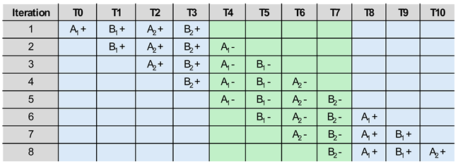 |
For an experiment with N=10000, this cycle must be repeated 1250 times. As a result, Alice and Bob generate identical copies of the input list, with pre-assigned values for all observables in each trial. (Though, we skipped the B values in Alice’s list, and the A values in Bob’s list, to simplify analysis). The next stage is to allow Alice and Bob to make random selections for each iteration. In practice, this means that they get to keep the values of the chosen observables (as prescribed by the random number generators) and ignore the other possible outcomes. After running the two simulations independently, the output lists are recombined by the moderator, effectively producing a reduced version of the input spreadsheet. For example, a cycle of 8 trials might look like this:
Table 3.
Possible output combinations for a full cycle of 8 input conditions.
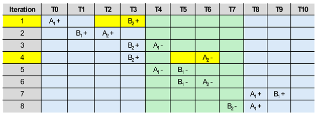 |
The two highlighted iterations (#1 and #4) contain distorted combinations. The two events of each pair are not consecutive on the table and therefore express pseudo-coincidences from different truncated windows. As a partial remedy, one of the two events (usually, the latest in time) must be subsequently deleted and replaced with a random binary value. All the other combinations are accepted as valid. This is an essential novelty of the presented model. In previous contributions to this topic, random events were treated as noise that can only weaken input correlations. Yet, our simulation is an ideal experiment where missing events arise exclusively from induced counter-correlations. Therefore, random events increase the observed correlations by restoring the input patterns that would otherwise be suppressed.
The final list of validated coincidences must be separated into four bins, according to the four types (A1-B1, A2-B1, A2-B2 and A1-B2). These dedicated lists can then be used to calculate the coefficients of correlation and to test the CHSH inequality. It is important to note that our moderator program (combine.py) performs no active coordination during the measurement phase. The scripts running on Alice and Bob execute completely in isolation, verifying that the physical events are Ontologically Local. The moderator's role is strictly passive, replicating the temporal coincidence-matching calculations performed by real-world laboratory computers post-experiment. Because the cyclic input structure is deterministic, repeated random seeds are not required to establish the asymptotic mechanism. They are useful, however, for quantifying finite-sample fluctuations arising from the independent setting randomizers and the replacement procedure. We therefore performed 5,000 independent simulations of 10,000 trials each. The mean CHSH value was S=3.0007, with a between-run standard deviation of 0.0265. The central 95% of individual runs fell between S=2.9484 and S=3.0521, and every run exceeded the local CHSH bound of 2. The four mean correlation coefficients approached +0.75,+0.75,+0.75, and −0.75, respectively. Increasing the number of trials reduced the standard deviation approximately as , while the mean converged to the analytically predicted value S=3.
The simulations were performed as described, using the code available in this public repository on GitHub: https://github.com/gmardari-owr/bell-experiment-two-computers. The repository contains the Python scripts, example input data, and instructions to reproduce the results.
5. Discussion
Mutually exclusive properties have many unexpected features. By default, they cannot coincide with each other as part of a single physical system. They can only be combined after the fact, across contexts, in fluid ways. Therefore, they cannot have objective coefficients of correlation. Instead, a single flow of events can be used to derive several patterns of pseudo-coincidence (or “subjective coincidence”), depending on the rule of combination. In the case of four observables, as needed for a CHSH experiment, it is possible to switch from compatible patterns (without Bell violations) to incompatible patterns of correlation (with Bell violations), simply by changing the number of events that are counted at the same time. As seen on the “wheel of fortune” set-up above, pairwise combinations can be fully consistent and still generate maximal Bell violations. Quadruple detections prevent the observation of such patterns, without any associated change in objective behavior. This shows that quantum monogamy can be explained as a combinatorial effect, without “spooky action at a distance”. Surprisingly, loophole-free experiments hide this process “behind the curtain”, since they require four events to be considered at each step, even if only two are recorded. This means that entangled quanta can violate the CHSH inequality, but cannot express this ability with ideal loophole-free protocols. Instead, they can only do so in real tests [8−11], where missing events are an essential feature. We invite the authors of these experiments to review their raw (unfiltered) time-tag data and to test the connection between injected randomness and observable coefficients of correlation.
Metaphorically speaking, Bell experiments are like riddles with several clues missing. For a long time, it was not known that quantum entanglement was monogamous (and therefore unable to produce loophole-free violations in ideal conditions). Likewise, it was not known that injected randomness can increase the likelihood of a Bell violation in realistic experiments. More importantly, it was not widely known that mathematical definitions of Locality were excessively narrow, expressing instead the ontological qualities of Simultaneous Realism. Convincing solutions did not seem possible for a long time, because all the missing clues had to be found at the same time. Nonetheless, for those looking for a silver lining, this can also be seen as a story in which two wrongs make one right. The founders of quantum mechanics were puzzled by non-commuting variables [41,42]. Do quantum momentum and position exist at the same time, or is this just an experimental appearance? John Bell discovered the right tool for a definitive answer, but framed it as a question about Locality. Because of this mistake, experimental loopholes received extraordinary attention, preventing the misinterpretation of quantum behavior. Then, loophole-free experiments were also mistaken for definitive tests of Locality, and thereby enabled the discovery of targeted effects from injected randomness. As a result, we now have a reliable tool for testing the nature of quantum non-commutativity, given the demonstrated ability to distinguish between genuine and spurious violations of the CHSH inequality. The unexpected conclusion is that non-commutativity and Causal Locality are compatible concepts. In other words, it is fair to interpret quantum theory as both correct and incomplete.
In conclusion, we discovered a programmable mechanism that produces strong CHSH violations in a simulated Bell experiment with two independent computers. Our model does not rely on communication between stations, but on the interaction between mutually exclusive observables and the protocol used to handle missing events. The implication is that Bell inequalities, contextuality, monogamy, and loophole-free experimental protocols have more subtle relationships than commonly understood. More broadly, this result highlights the need to examine how measurement procedures themselves can influence the statistical structures used to characterize physical systems.
Acknowledgements
France Čop wrote the code for the simulation but humbly declined to be listed as a co-author.
Code and data availability
The full code, example data, and instructions to reproduce the results are openly available on GitHub: https://github.com/gmardari-owr/bell-experiment-two-computers. The archived version used in this paper has DOI: https://doi.org/10.5281/zenodo.21246897.
References
- Bell, J. S. On the Einstein-Podolsky-Rosen Paradox. Physics 1964, 1, 195. [Google Scholar] [CrossRef]
- Bell, J. S. Speakable and Unspeakable in Quantum Mechanics; Cambridge, 1987. [Google Scholar]
- Fine, A. Joint distributions, quantum correlations, and commuting observables. J. Math. Phys. 1982, 23, 1306. [Google Scholar] [CrossRef]
- Cetto, A. M.; Valdés-Hernández, A.; de la Peña, L. On the Spin Projection Operator and the Probabilistic Meaning of the Bipartite Correlation Function. Found. Phys. 2020, 50, 27. [Google Scholar]
- Dhar, H. S.; Pal, A. K.; Rakshit, D.; Sen (De), A.; Sen, U. Monogamy of Quantum Correlations - A Review. In Lectures on General Quantum Correlations and their Applications; Fanchini, F., Soares Pinto, D., Adesso, G., Eds.; Springer, 2017. [Google Scholar]
- Mardari, G. N. Quantum Monogamy with Predetermined Events. Quantum Rep. 2025, 7, 62. [Google Scholar] [CrossRef]
- Khrennikov, A. Bell-Boole Inequality: Nonlocality or Probabilistic Incompatibility of Random Variables? Entropy 2008, 10, 19. [Google Scholar] [CrossRef]
- Hensen, B.; et al. Loophole-free Bell inequality violation using electron spins separated by 1.3 kilometres. Nature 2015, 526, 682. [Google Scholar] [CrossRef] [PubMed]
- Giustina, M.; et al. Significant-loophole-free test of Bell's theorem with entangled photons. Phys. Rev. Lett. 2015, 115, 250401. [Google Scholar] [CrossRef] [PubMed]
- Shalm, L. K.; et al. A strong loophole-free test of local realism. Phys. Rev. Lett. 2015, 115, 250402. [Google Scholar] [CrossRef] [PubMed]
- Rosenfeld, W.; et al. Event-Ready Bell Test Using Entangled Atoms Simultaneously Closing Detection and Locality Loopholes. Phys. Rev. Lett. 2017, 119, 010402. [Google Scholar] [CrossRef] [PubMed]
- Pearle, P. M. Hidden-Variable Example Based upon Data Rejection. Phys. Rev. D. 1970, 2, 1418. [Google Scholar] [CrossRef]
- Larsson, J._A. Bell's Inequality and Detector Inefficiency. Phys. Rev. A 1998, 57, 3304. [Google Scholar] [CrossRef]
- Larsson, J. Loopholes in Bell inequality tests of local realism. J. Phys. A 2014, 47, 424003. [Google Scholar] [CrossRef]
- Clauser, J. F.; Horne, M. A.; Shimony, A.; Holt, R. A. Proposed Experiment to Test Local Hidden-Variable Theories. Phys. Rev. Lett. 1969, 23, 880. [Google Scholar] [CrossRef]
- Mardari, G.N. Quantum Correlations in Classical Systems. Quantum Rep. 2026, 8, 35. [Google Scholar] [CrossRef]
- Popescu, S.; Rohrlich, D. Quantum Nonlocality as an Axiom. Found. Phys. 1994, 24, 379. [Google Scholar] [CrossRef]
- Raymond-Robichaud, P. The equivalence of local-realistic and no-signaling theories. Preprint 2017, arXiv:quant. [Google Scholar] [CrossRef]
- Raymond-Robichaud, P. L’équivalence entre le local-réalisme et le principe de non-signalement. PhD Thesis, Université de Montréal, 2017. Available online: https://papyrus.bib.umontreal.ca/xmlui/handle/1866/20497.
- Vorob’ev, N. N. Consistent Families of Measures and Their Extensions. Teor. Ver. Prim. 1962, 7, 153. [Google Scholar] [CrossRef]
- Hess, K.; Philipp, W. A Possible Loophole in the Theorem of Bell. Proc. Natl. Acad. Sci. USA 2001, 98, 14224. [Google Scholar] [CrossRef] [PubMed]
- Hess, K.; Philipp, W. Bell’s Theorem: Critique of Proofs with and without Inequalities. AIP Conf. Proc. 2005, 750, 150. [Google Scholar] [CrossRef]
- la Pena, L. de; Cetto, A. M.; Brody, T. A. On hidden variable theories and Bell’s inequality. Lett. Nuovo Cim. 1972, 5, 177. [Google Scholar] [CrossRef]
- Nieuwenhuizen, T. M.; Spicka, V.; Mehmani, B.; Aghdami, M. J.; Khrennikov. A. Y. (eds): Beyond the Quantum; World Scientific, 2007. [Google Scholar]
- Nieuwenhuizen, T. M. Is the contextuality loophole fatal for the derivation of Bell Inequalities? Found. Phys. 2011, 41, 580. [Google Scholar]
- Khrennikov, A. Beyond Quantum; Pan Stanford Publishing, 2014. [Google Scholar]
- Jung, K. Violation of Bell's Inequality: Must the Einstein Locality Really be Abandoned? J. Phys. Conf. Ser. 2017, 880, 012065. [Google Scholar] [CrossRef]
- Khrennikov, A. Get Rid of Nonlocality from Quantum Physics. Entropy 2019, 21, 806. [Google Scholar] [CrossRef] [PubMed]
- Hess, K. A. Critical Review of Works Pertinent to the Einstein-Bohr Debate and Bell’s Theorem. Symmetry 2022, 14, 163. [Google Scholar] [CrossRef]
- Mardari, G. N. Experimental Counterexample to Bell’s Locality Criterion. Entropy 2022, 24, 1742. [Google Scholar] [CrossRef] [PubMed]
- Cetto, A.M. Electron Spin Correlations: Probabilistic Description and Geometric Representation. Entropy 2022, 24, 1439. [Google Scholar] [CrossRef] [PubMed]
- De Raedt, H.; Katsnelson, M. I.; Jattana, M. S.; Mehta, V.; Willsch, M.; Willsch, D.; Michielsen, K.; Jin, F. Einstein–Podolsky–Rosen–Bohm Experiments: A Discrete Data Driven Approach. Ann. Phys. 2023, 453, 169314. [Google Scholar] [CrossRef]
- Geurdes, H. Bell’s Theorem and Einstein’s Worry about Quantum Mechanics. J. Quant. Inf. Sci. 2023, 13, 131. [Google Scholar] [CrossRef]
- Kupczynski, M. Quantum nonlocality: How does Nature do it? Entropy 2024, 26, 1. [Google Scholar] [CrossRef] [PubMed]
- De Raedt, H.; Katsnelson, M. I.; Jattana, M. S.; Mehta, V.; Willsch, M.; Willsch, D.; Michielsen, K.; Jin, F. Can Foreign Exchange Rates Violate Bell Inequalities? Ann. Phys. 2024, 469, 169742. [Google Scholar] [CrossRef]
- Kay, A. F. Escape from Shadow Physics; Basic Books: NY, 2024. [Google Scholar]
- Aspect, A.; Dalibard, J.; Roger, G. Experimental test of Bell’s inequalities using time-varying analyzers. Phys. Rev. Lett. 1982, 49, 1804. [Google Scholar] [CrossRef]
- Coffman, V.; Kundu, J.; Wootters, W. K. Distributed entanglement. Phys. Rev. A 2000, 61, 052306. [Google Scholar] [CrossRef]
- Koashi, M.; Winter, A. Monogamy of quantum entanglement and other correlations. Phys. Rev. A 2004, 69, 022309. [Google Scholar] [CrossRef]
- Osborne, T. J.; Verstraete, F. General Monogamy Inequality for Bipartite Qubit Entanglement. Phys. Rev. Lett. 2006, 96, 220503. [Google Scholar] [CrossRef] [PubMed]
- Einstein, A.; Podolsky, B.; Rosen, N. Can Quantum-Mechanical Description of Physical Reality Be Considered Complete? Phys. Rev. 1935, 47, 777. [Google Scholar] [CrossRef]
- Bohr, N. Can Quantum-Mechanical Description of Physical Reality Be Considered Complete? Phys. Rev. 1935, 48, 696. [Google Scholar] [CrossRef]
Figure 1.
“Wheel of fortune” toy model for the study of incompatible properties. Several patterns of subjective coincidence can be extracted from a single record of events. (a) The same cycle of 8 mutually exclusive outcomes is repeated continuously, as the table spins under a fixed arrow. Rotation can stop at any of the 8 possible markers (0−7), enabling “at will” measurements with random settings. (b) Overlapping pairwise measurements across time that can produce maximal CHSH violations. (c) A scheme with quadruple detections produces an automatic rearrangement into a pattern without violations.
Figure 1.
“Wheel of fortune” toy model for the study of incompatible properties. Several patterns of subjective coincidence can be extracted from a single record of events. (a) The same cycle of 8 mutually exclusive outcomes is repeated continuously, as the table spins under a fixed arrow. Rotation can stop at any of the 8 possible markers (0−7), enabling “at will” measurements with random settings. (b) Overlapping pairwise measurements across time that can produce maximal CHSH violations. (c) A scheme with quadruple detections produces an automatic rearrangement into a pattern without violations.
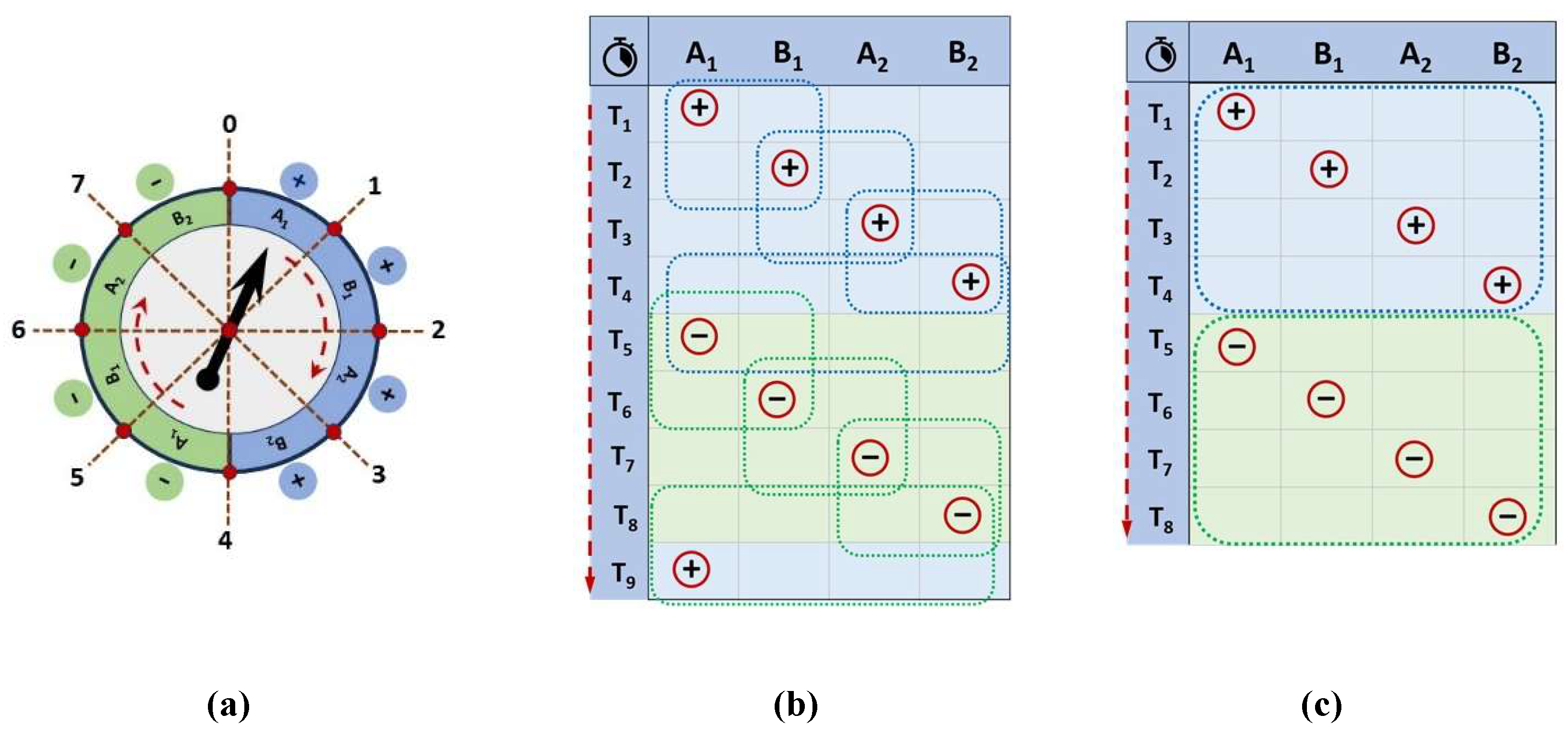
Figure 2.
Visual illustration of possible correlation patterns in different measurements scenarios with mutually exclusive properties. (a) Overlapping pairwise measurements can produce a Möbius strip pattern with three correlations and one anti-correlation. Maximal Bell violations (S=4) are possible. (b) Global measurements introduce a counter-correlation that breaks off the crossover connections between A1 and B2. Bell violations become impossible (S≤2). (c) Coincidence windows can identify displaced events. Random replacement produces a 50-50 mixture between the two possible patterns, revealing suppressed violations up to S=3.
Figure 2.
Visual illustration of possible correlation patterns in different measurements scenarios with mutually exclusive properties. (a) Overlapping pairwise measurements can produce a Möbius strip pattern with three correlations and one anti-correlation. Maximal Bell violations (S=4) are possible. (b) Global measurements introduce a counter-correlation that breaks off the crossover connections between A1 and B2. Bell violations become impossible (S≤2). (c) Coincidence windows can identify displaced events. Random replacement produces a 50-50 mixture between the two possible patterns, revealing suppressed violations up to S=3.
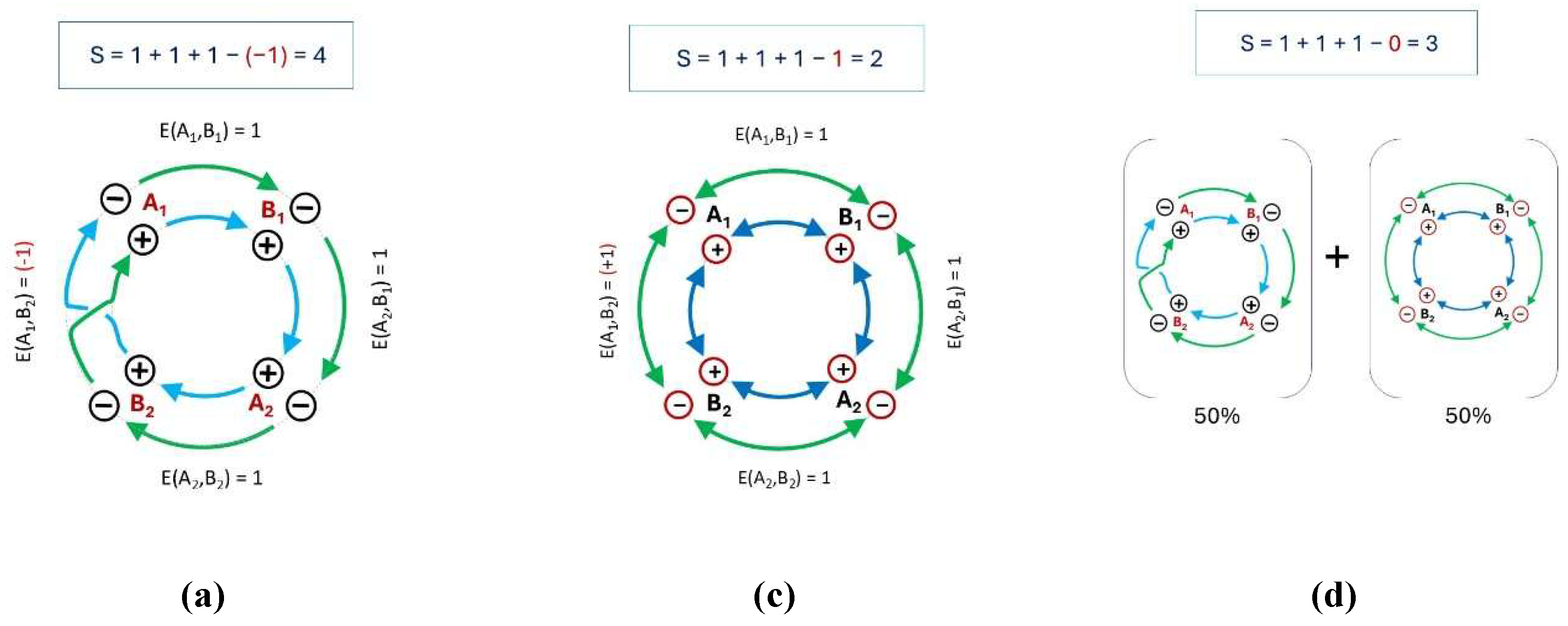
Table 1.
Effect of replaced missing events on loophole-free Bell violations.
| Proportion of Corrected Outcomes | Resulting CHSH Value (S) | Violation Level |
| 0 | None (Monogamy Bound) | |
| 1/32 (~3.1%) | Moderate Violation | |
| 1/16 (~6.2%) | Strong Violation | |
| 1/8 (~12.5%) | Super-Quantum Violation |
Disclaimer/Publisher’s Note: The statements, opinions and data contained in all publications are solely those of the individual author(s) and contributor(s) and not of MDPI and/or the editor(s). MDPI and/or the editor(s) disclaim responsibility for any injury to people or property resulting from any ideas, methods, instructions or products referred to in the content. |
© 2026 by the authors. Licensee MDPI, Basel, Switzerland. This article is an open access article distributed under the terms and conditions of the Creative Commons Attribution (CC BY) license (http://creativecommons.org/licenses/by/4.0/).
Copyright: This open access article is published under a Creative Commons CC BY 4.0 license, which permit the free download, distribution, and reuse, provided that the author and preprint are cited in any reuse.


