

Submitted:
22 July 2026
Posted:
22 July 2026
You are already at the latest version
Abstract
This study evaluates the effects of sampling interval and averaging period on the assessment of extreme mean wind speeds for structural design, focusing on correction factors for the standard meteorological observations that are archived for more than 35,000 stations around the globe. A literature review reveals insights and flaws in past works that influenced the design of the two phases of the study. The first phase uses 2-minute mean wind speeds at 1-minute intervals over, typically, 20 years from 642 well-exposed stations distributed over the contiguous USA that are averaged to the World Meteorological Organization standard ten-minute and hourly means. Informed by the first stage results, which confirms good representation by the Weibull distribution with a von Karman autocorrelation, the second phase uses simulated 1,000-year timeseries to investigate the parameters governing the effects, which are: sampling interval, averaging period, integral timescale of the autocorrelation, and the return period of the extremes. The effects of these four parameters, in any combination, consolidate into a single analytical equation with empirically calibrated coefficients which is a good match well to the empirical analysis of the first phase, when using the appropriate integral time scale.
Keywords:
sampling interval
; averaging period
; extremes
; timeseries simulation
; Weibull distribution
; von Karman autocorrelation
; integral time scale
; mixed wind climate
1. Introduction
Extreme wind speeds for the design of structures are typically assessed by extreme-value analysis (EVA) of wind speeds observed at 10m above ground level in flat open country and embodied into codes of practice and other design guidance, e.g. as in [1]. The accuracy of these empirical assessments depends on many factors, including the characteristics of the anemometers, their exposure in terms of upwind roughness changes and their density over the geographical region. More recently, synoptic-scale wind speeds have been deduced at the surface from the atmospheric pressure fields of reanalysis models [2], again at hourly intervals, developed from the pioneering study by [3] – a methodology that resolves issues of geographical cover.
Most anemometers are situated at airports, reporting mean and maximum gust speed and direction over a 10-minute period at hourly or, latterly, ½-hourly intervals to the World Meteorological Organization (WMO) standards. Reports are archived for more than 35,000 stations around the globe in the US National Centers for Environmental Information (NCEI) Global Hourly, Integrated Surface Data (ISD), dataset DS3505 1. These standard reports are under-sampled (disjoint), as they omit the wind speeds occurring in the 50, or 20, minutes between the reports. Some meteorological authorities also make contiguous observations, e.g. mean and maximum gust values over a one-hour period at hourly intervals, so that no gust speeds are lost but it is still possible to miss a higher average wind speed that spans across intervals. The WMO standards (FM12 SYNOP and FM15 METAR) report wind speed in integer knots (1kn = 0.5144ms-1) and directions in 10° increments but, to accommodate speeds in other units, DS3505 archives speeds in integer 0.1ms-1 increments (e.g. 20kn is archived as 103). Contiguous hourly-mean observations for the UK are available in the Met Office MIDAS Open database hosted by the Centre for Environmental Data Analysis 2. Starting in 1998 at a few stations and implemented at more than 800 stations by 2004, the US Automated Surface Observation System (ASOS) provides observations of the 2' mean and the maximum 5" gust speed and direction at 1' intervals in the ISD dataset DS6405 3 and is currently the only readily accessible dataset sampled at such a high rate.
National and international codes of practice differ in their definition of extreme wind speeds for the design of structures. The UK was the first to move to a probabilistic basis with the introduction of a 3-second gust speed with a 50-year return period [4] on the basis that gust speeds were thought to be less affected by ground roughness than mean speeds. However, extreme gust speeds are much more likely than mean speeds to include high-value artefacts and just one artefact per year can dominate the EVA [5]. With the development of an atmospheric boundary layer model for heterogeneous terrain [6], allowing reliable exposure corrections for mean speeds, the UK moved to hourly-mean speeds applied with a gust factor model for gust speeds [7]. Development of the Eurocodes led to the adoption of 10-minute mean wind speeds [8] as the datum which aligns with the WMO observational standards. Each of these different definitions remain in force somewhere around the globe.
This present study focuses on two principal issues: a) the effect of averaging period and b) the effect of sampling interval on the assessment of extreme mean wind speeds, specifically on , the -year return speed averaged over time . Resolving the first issue enables transformation of values between averaging periods and resolving the second issue allows underestimates of peak speeds to be corrected. The essence of these issues is illustrated in Figure 1 which presents typical 5h traces of: (a) and (b) , running mean wind speed at intervals by the ◯ (circle) symbols. Note that wind speed units are maintained in the original observed WMO standard of knots (1kn = 0.5144ms-1) throughout this study to avoid unit conversion bias [5]. For the running mean in (a), contiguous sampling at intervals is shown by the thin (red) line, and disjoint sampling at intervals by the thick (blue) line. It is evident that the disjoint samples miss the central peak speed as well as the short-duration (mesoscale) peak at minute 63, while the contiguous samples slightly underestimate these peaks. For the running mean in (b), the short-duration peak is suppressed by the running mean and contiguous sampling at intervals underestimates the central peak by a larger amount. In sampling a continuous timeseries the probability of missing a peak is controlled by the relative timescale, defined here as the disjoint sampling ratio:
Hence represents disjoint sampling, contiguous sampling, and over-sampling. For the ASOS DS6405 -interval wind speeds, and , which are the closest to continuous that can be achieved with the ASOS observations.
The remainder of this paper is organized as follows: §2 is a review and discussion of relevant previous studies; informing §3 which describes the models, methods and data used in the two stages of this study; §4 presents the results of each stage with relevant discussion, and finally; §5 assembles and discusses the conclusions of the study which are summarized by the bullet points in §6.
2. Review of Previous Studies
Previous studies of these issues are reviewed chronologically to take account of insights and flaws that are addressed, or not, by later studies:
1. In [9] a new wind map was proposed for Italy for to the Eurocode standard. This was based on EVA of for 42 stations at intervals and for 27 stations at intervals, corrected for exposure. Preliminary studies suggested that the 3-hour interval underestimates in the range 5% to 10%;
2. In [1], proposing a new zonal wind map for Germany, a factor of was applied to transform from hourly-mean observations, , into the Eurocode standard ten-minute mean, , without revealing the source of this value. The study included thunderstorm downbursts and gust fronts in addition to the synoptic scale windstorms, fitting only the (least reliable) far-right tail of the EVA distribution of this mixture to evaluate the dominant component in any given location. The study proposed an optimum sample size, , defining the rank of lowest observation as given by . This resulted in fewer fitted observations than recommended by [10] for the XIMIS EVA method, but was necessary to isolate the dominant component of the mixed wind climate;
3. The [3] study was the first to derive extreme wind speeds at the surface from maps of sea-level atmospheric pressure and was the inspiration for the rapid development of this technique into using re-analysis models, e.g., [2]. 489 individual storms with a central pressure below 970mbar were selected to represent the most intense storms affecting Europe between 1953 and 1995. Geostrophic wind speeds in time steps over a 0.5° interval grid covering Europe were evaluated by linear interpolation between the 6h-interval maps over the lifetime of each storm. 50-year return geostrophic speeds were estimated by the peaks-over-threshold (POT) method and transformed to surface wind speeds using the geostrophic drag law. The principal advantage of this approach is that the surface wind speed is predicted everywhere in the field to the same resolution, which is particularly valuable where anemometer stations are sparse;
4. Study [11] focused on the principal issues of the present study: empirically through observations and theoretically when modelled as a Gaussian Markov chain. Empirical assessments of averaged speeds at 5 locations in Denmark and 3 locations in the Arabian Gulf were made in terms of the mean of the observed annual maxima. Attenuation factors were evaluated for sample intervals from to and for averaging periods, , over the same range – apparently assuming the two effects to be mutually independent. Evaluating their empirical fits to the relevant averaging times and sample intervals indicates that the factor for from is , compared with 1.06 from [1], and that sample intervals underestimate yearly maxima by 3.1% and intervals by 6.0%. The principal deficiency of the Markov model is that each new value depends only on the previous value, whereas wind speeds have a memory of previous values over several hours, as expressed by the integral timescale, , of their autocorrelation
5. Study [12] addressed three issues: 1 – The starting wind speed of anemometers; 2 – The appropriate extreme-value distribution; and 3 – The averaging time and sampling interval between observations. The first issue was demonstrated to have no significant effect on extremes and, in any case, the starting speed of the latest generation of fast-response cup-anemometers is very much improved and is effectively zero for sonic anemometers. While debate over the second issue continues, the argument against asymptotic models and in favor of the sub-asymptotic, or “penultimate” form of the Fisher-Tippet Type 1 (FT1), or Gumbel distribution is demonstrated by the latter’s effectiveness in the XIMIS method [10,13]. Hence the only third issue of averaging time and sampling interval is relevant to the present context. The empirical analysis was similar to [11], starting with mean wind speeds at hourly intervals, re-sampling at longer intervals, 2, 3, 4, 6, 8, 12 and 24h, then extrapolating a regression fit back to contiguous intervals. They claimed that intervals represent the theoretical limit value, but this neglected the underestimation of continuous running averages by contiguous averages illustrated in Figure 1. They concluded that the correction factor to contiguous average speeds from , and intervals was 1.03, 1.05 and 1.08, respectively;
6. Study [14] was the first to exploit the interval observations in DS6405, comparing hourly means from interval, average, DS6405 data to the mean from DS3505 at hourly intervals at 8 US stations. It claimed an 8% – 38% overestimate of by DS3505 “due to large discrepancies” in DS3505. The DS3505 observations for these stations are typical hourly reports compiled from the DS6405 data over the averaging period, between and before each hour, so are averages and not averages, as was assumed. One principal contribution to the overestimates is therefore the missing transformation factor [1]. Another is that the average includes mesoscale convective events which are suppressed by the average. The short observation period of 14 years leads to inherent overestimation of by EVA due to statistical variance. These effects do not explain the largest overestimates, but EVA is notoriously susceptible to any high-valued artefacts in the record. The “extensive QA/QC process” of this study was not explained but needed to have been rigorous, as in [5]. Additional procedures have since been developed to identify and correct frequent artefacts particular to the ASOS DS6405 data [15]. The study gave the first estimate for the slight increase in the rolling hourly average (continuous) over the block hourly average (contiguous) of 2% – 3%;
7. Study [16] used Monte-Carlo simulations of Weibull parents by the [17] method, using the probability density and spectrum obtained from DS6405 data at each of 6 stations in central USA to obtain simulated records of 18,000y because “the combined effect of the sample size and disjunct sampling cannot be well understood by only using one set of data with limited years of observation”. The locations were chosen to avoid hurricane contributions, and the observations were stripped of thunderstorm events indicated by the DS3505 “present weather” codes. The study claimed that the Gaussian Markov chain model in [11] overpredicted the effect of disjunct sampling for averages at large sample intervals. It predicted that the factor from intervals to contiguous intervals is , and to intervals is (where the latter can be regarded to be effectively a continuous running average). The study concluded that the effect of disjunct sampling depends only on the disjoint ratio, (Equation 1);
8. Study [18] reviewed the previous studies, above, and concluded that none were “satisfactory and reliable”, being particularly critical of the Gaussian process and zero-memory Markov assumptions in [11] and of the accuracy of the extrapolation to contiguous sampling in [12]. The study used contiguous average wind speeds at 117 stations across Germany to calibrate a closed-form equation relating yearly maxima, , to disjoint samples, confined specifically to synoptic storms, of the form:
where is the correction factor, and are empirical values to be fitted. Two issues with Equation (2) are that the datum for was , contiguous not continuous, and the boundary conditions as (continuous) are not met. In calibrating Equation (2) it was assumed that the average eliminated contributions from thunderstorm events, but their influence is only reduced. The fitted values had no geographical correlation, leading to and as being applicable to the whole of Germany, with . Other useful values emerged from the data, including the Weibull shape factor which is comparable to UK values [19];
The chronologically evolving estimates of the transformation factors and for , summarised in Table 1, show consistent trends, but inconsistent values. Having critically reviewing earlier work, the values of proposed by [18] are considerably larger. A third relevant timescale is absent from all the previous studies: the integral timescale, , derived from the autocorrelation, , by integration or by fitting an appropriate model. This may account for the variation in values for the same between locations in different wind climates.
Most of the previous studies focus on synoptic-scale events. By including the annual and daily harmonics in the spectra, the simulation in [16] by the [17] spectral method raises a fundamental issue. Spectra are formed by an integral-average through time which also removes all phase information, so that simulations generated using [17] method are forced to be stationary and so the harmonics are resolved homogeneously through time as cycles of constant amplitude and unknown phase. The phase of the fundamental harmonics can be deduced from the physics, but not the Oort and Taylor [20] sidebands that represent the seasonal modulation of the diurnal cycles. This creates anomalies in the simulated timeseries, including negative velocities at night in periods of relative calm, as the diurnal cycles have the same amplitude at all wind speeds. This is incompatible with the current understanding that each wind climate is caused by several meteorological mechanisms which, when examined in a seasonal-diurnal analysis, resolve into a disjoint mixture of phase-locked, amplitude-modulated random components [21,22]. By working in the time domain, so preserving phase, only the Harris methodology is currently capable of simulating the seasonal-diurnal components of a disjoint mixture [23].
3. Materials and Methods
The present study addressed the issues empirically by analyzing observations, and parametrically by analyzing long-period simulations, using the ASOS parameters: averages and sampling intervals as the datum, while taking due account of insights gathered from the earlier studies. All analyses of this study were implemented in the R statistical computing language, Version 4.4.1 (https://cran.r-project.org/).
3.1. ASOS Observations
The ASOS observations from 2000-2003 to 2023 at intervals for the 642 well-exposed stations across the contiguous USA (CONUS) in Figure 2, were downloaded from the ISD dataset DS6405. The stations were all at airports and are identified by their unique International Civil Aviation Organization (ICAO) 4-letter codes, e.g. KBOS for Boston, Logan International Airport. Following the approach of [24] and earlier studies, observations that might have come from hurricanes were removed over the three-day period centered on landfall, initially just at stations in the landfall States. Owing their rarity, hurricanes and tropical cyclones are assessed separately from other synoptic-scale storms, in terms of their characteristics as a class and their likelihood of occurrence derived from observations of their tracks [25]. This methodology has been recently extended to assess the action of severe North Atlantic depressions across Europe [26]. Secondly, all the convective gust events >20kn and non-meteorological artefacts from the [27] dataset of classified convective gust events were removed over the period centered on the peak speed, so as to retain only the synoptic class. The later EVA analysis exposed potential non-synoptic artefacts remained at only 74 of the 642 stations, all of which were examined manually, and confirmed artefacts were removed as reported in §3.4.
The standard and averaging was applied to the interval observations by a running block-average, after which the observations were re-sampled at , and intervals. Re-sampling was repeated in subsets offset by intervals to maximise the available information in the observations. For example, provided 60 subsets of observations for analysis, albeit mutually correlated.
3.2. Autocorrelations and Integral Timescales
Autocorrelations (non-dimensional) and autocovariances (dimensional) are tolerant of missing observations, whereas Fourier transformations for the spectra are not. Here the autocovariances were evaluated up to a maximum lag of 2 years after resampling at intervals to limit the computational overheads. Accounting for leap years by the average of 356.25 days per year, exactly 2 years ensured an integer number of ½-daily cycles and two whole annual cycles, ensuring that the integral timescales, , were effectively the same with or without inclusion of the daily/annual harmonics.
Example results for KBOS, Boston, MA, are shown in Figure 3(a) for the first 10 days and (b) for the whole 2 years of lags. Figure 3(c) shows the autocovariance after removal of the harmonics by heterodyning [28], together with the best regression fits to the von Karman (vK) autocorrelation model, with its fixed 5/3 decay constant, and the bandwidth-limited pink noise (BLPN) model, introduced in [23] as a “universal replacement” for vK, since this allows for a variable decay constant and the limited bandwidth set by the averaging time, . Both models are good fits to the observed autocovariance and are virtually indistinguishable in the rapid decay towards the origin, justifying the use of the simpler vK model in §3.5. This provided three estimates for the integral timescale, , which are mutually consistent, but around half the value found by [28] in the UK.
The integral timescale, , is the scaling factor for time that normalizes the autocorrelation function with respect to time lag, and the corresponding spectrum with respect to frequency, into standard expressions. Neither of the other two time-dimensioned parameters, and , are timescales in the conventional sense. The observation period, , sets the population of independent peaks available for EVA, so controls the statistical variance of the results. The return period, , is just a convenient proxy for the annual probability of exceedance, , i.e., .
3.3. Weibull Analysis
The classic Weibull analysis of the observed wind speeds is relevant because the index, , controls the rate of convergence of extremes to the FT1 distribution [29]. The scale and index parameters of the Weibull distribution:
were estimated by regression after linearization to:
Following [30], , is the cumulative probability of after removal of calms. The classical Weibull plot of against derives from the slope and from the intercept of a linear fit to Equation 4. The example in Figure 4(a) for Boston, MA, happens to be an excellent fit, helped by the 60-fold increase in observations at 1’ intervals as opposed to the more typical 60’ intervals, and the reduction in statistical variance this provides. But not all stations fitted quite this well. Figure 4(b) shows the probability density function (PDF) of for all stations at each of the averaging periods, with the corresponding ensemble mean, , and standard deviation, .
3.4. Extreme-Value Analysis
XIMIS [10] was adopted as the EVA method in this study because [13] recently demonstrated it to be the most reliable of the available methods for this context. XIMIS allows for incomplete convergence to the FT1 [29] distribution, for left-censoring of the peaks, for inverse variance weighting of the fit, and for preconditioning to maximize convergence to the penultimate FT1 model:
Here, is the reduced variate [29], is the mode, is the dispersion, and the convergence index is the index of the parent Weibull distribution [10].
Following experience over the last two decades in the use of XIMIS for supervised fitting, the left-censoring threshold was set to admit a maximum of 50 ranks (2½ times the observation period), but not more than half of the independent peaks. This allowed automated fitting to proceed unsupervised, which was essential given the huge number of fits required. The independent peaks in each subset were selected as the largest value occurring in the period between up/down-crossings of the mean speed, as illustrated in Figure 5, following the principle introduced by Davenport [31] in his adaption of the communication theory of Rice [32]. This predicts that there is one, and only one, statistically independent peak value between each successive up-crossing of the mean. As in [33], the running 100s mean was used to clearly define the mean-crossings. The Boston example in Figure 5 (a) illustrates the integer knot values of the reported mean, contrasting with the fractional values in (b) for the Rayleigh simulation. Figure 5(b) demonstrates the action of ensuring independence from adjacent peaks, showing that the secondary peaks either side of the highest are excluded because they occur between the same mean-crossings. The smaller peaks within their own mean-crossing periods on either side contribute, although they may subsequently be excluded by the left-censoring threshold of XIMIS.
XIMIS was applied at all ASOS stations for and , using: a) the station values of ; b) and 1.8, the means from Figure 4(b); and c) , the Rayleigh value [34]. Figure 6 shows example XIMIS analyses for at KBOS, Boston, MA, as classical Gumbel plots, . The ranked peaks for each fitted sub-set are shown by the + (red) symbols, the ensemble mean for each ranked subset by the ◯ symbols and their fit by XIMIS with by the thick curve. The outer chained curves are the 5%/95% confidence limits for the individual values, and the thin (red) curves are the 5%/95% confidence limits for values predicted from the fit. In the left-hand chart for there is only one subset, so + and ◯ are coincident, but in the right-hand chart there are 60 subsets. The most volatile fits are for and because there is only one subset, so no ensemble to average. 74 stations (~12%) had outliers above the 95% confidence limit and, as recommended by Gumbel [29], these were individually checked. Most cases were found due to erroneous values, convective gusts <20kn, or events that evaded the quality control procedure, so that they were excluded from analysis. This left 20 valid single outliers (~3% of the stations) for due to short-duration (mesoscale) events, reducing them to 5 single outliers (~1% of the stations) for as the additional averaging suppressed these events. These were retained to be addressed by the inverse variance weighting of XIMIS.
Ensemble averages were compiled of the mode and dispersion parameters in Equation (5) and of evaluated from the individual fits for each subset. As Equation (5) is linear in terms of each parameter value raised to the same index, , it follows that , allowing to be evaluated for any other return period from , and the associated .
3.5. Simulation Method
The principal role of the second stage simulation was to examine the issues parametrically, using very long simulated time series to minimize statistical variance, and to evaluate how the parameters scale. Available simulation methods were the two time-domain methods of Harris: [35] for Rayleigh (), [36] for Weibull with general index, and the more generalized spectral method of Nichols et al [17]. The choice need to keep the overall computation time within practical limits, requiring a compromise between best representation and speed. The Rayleigh method is the fastest, matching the target parameters in a single pass and its index, , lies within the upper quartile for the ASOS stations, Figure 4(b). The computation time using either of the other methods would have been prohibitive. A secondary role of the simulation was to investigate the case of zero averaging period, , which is impossible from station observations as all include some degree of averaging.
Simulations of 1,000 years of wind speed were generated by the Rayleigh [35] simulation method at intervals for vK autocorrelations with a range of integral timescales, This method exploits the fact that a Rayleigh timeseries, may be formed as the orthogonal resultant of two Gaussian timeseries and that linear operations on Gaussian timeseries remain Gaussian, e.g., when applying an autoregressive (AR) filter. The required autocorrelation was evaluated, then transformed into AR filter coefficients by the Yule-Walker equations [37] which, when applied to the two Gaussian random timeseries, resulted in a Rayleigh-distributed timeseries with vK autocorrelation with the desired timescale, . The same initial Gaussian streams were used to simulate each different timescale and averaging period to allow direct comparison between simulations and for compatibility with the empirical ASOS data. The simulation produced values normalized to unity mean.
Although the 1,000-year period was shorter than the 18,000 years used by [16], it proved quite adequate for the purpose, and allowed sub-division into independent observation periods, y, 20y, 50y and 100y to emulate the range of observations found in practice, additional to the correlated sets. For example, with y and , typical of DS3505 data, there were 50 independent sets, each of 60 correlated subsets for EVA, requiring 3,000 XIMIS fits.
4. Results
4.1. ASOS Observations
4.1.1. Integral Timescales
The integral timescale, , is the time-domain scaling factor for any given autocorrelation function. Figure 7 presents the relevant results of the ASOS autocorrelation analysis as color-mapped contour maps of CONUS, where: (a) for vK and (b) for BLPN show that the integral timescale, , has a consistent geographical pattern with most variation in the high-topography western ⅓ of the USA and along the Gulf coast. Figure 3(c) showed an excellent match between vK and BLPN autocovariances for Boston, which is typical for all stations, with Figure 7(c) showing <10% difference overall and <2% difference over the eastern ⅔ of the USA. The BLPN decay constant, Figure 7(d) shows a similar pattern, but shows a gradient with latitude over the eastern ⅔.
Figure 8 investigates the BLPN decay index at stations east and west of longitude −100°. In (a) the PDFs are seen to separate into two distinct, but overlapping, distributions where the mean for the east stations is indistinguishable from the vK value of 5/3 but is significantly lower for the west stations. Note that each distribution shows a ripple matching the mode of the other, indicating some ‘leakage’ either side of longitude −100°. In (b), the quantile-quantile (Q-Q) plot shows a very small correlation between integral timescale and decay index, and that the difference between the all-station mean, 1.53, and the vK value is small compared with the range of scatter. Note that the four station values in the top left corner of (b) were taken to be invalid outliers and were excluded from the contour maps in Figure 7.
4.1.2. Weibull Parameters of Parent Wind Speeds
The Weibull index values are relevant to justify using the Rayleigh simulations with . The PDFs in Figure 4(b) show that the ensemble mean, for all stations, increases with averaging period, . This is interpreted as progressive elimination of shorter duration events as increases. The average includes contributions from the micrometeorological range of the atmospheric boundary layer (ABL) spectrum [38] which are progressively eliminated by the and averages which define the boundaries of the mesoscale range, the so-called Spectral Gap, so the residual mesoscale components for are eliminated by Even so, with only synoptic-scale components, , which is still less than the ideal Rayleigh value predicted by Offset Elliptical Normal (OEN) model theory [19,39]. However, the synoptic-scale wind speed remains a mixture of disjoint components, typically cyclonic and anticyclonic systems. Figure 11 of [13] demonstrates how the index of a single Weibull distribution will present in the range for a disjoint mixture of two Rayleigh components, depending on their relative frequency. The ranges of the PDFs in Figure 4(b) are much greater than the differences in .
Figure 9(a) maps the geographical distribution of , showing lower values in the eastern and western ⅓ and higher values in the middle. The pattern for is not shown because it is virtually identical (with 98% correlation and 0.042 standard error). In Figure 9(b), the Q-Q plot for , the regression slope (solid line) matches the corresponding ratio of in Figure 4(b), and the dashed lines are the 5%/95% confidence limits on the standard error. The high correlation and small standard error indicate that this observed geographical variation is real.
4.1.3. Extreme Wind Speeds
The previous assessment of the reliability of EVA [13], showed XIMIS to be the most reliable when the index, , in Equation (4) takes a fixed value, i.e. when using a two-parameter fit instead of a three-parameter fit, because fitting with as a free parameter is poorly conditioned. But the question remains, which value? The geographical variation of station values in Figure 9(a) is inconvenient when seeking a universal solution for mapping, and their mean values depend on averaging period, . The Rayleigh value is convenient in allowing direct comparisons with the Harris simulation model [35] of §3.2 but, more importantly, because that is predicted by the theory of the OEN model [19,39] and is expected to control the curvature of an OEN mixture distribution in the upper tail.
This question was resolved pragmatically by correlating for the individual station indices and the ensemble-mean for all stations, using the Rayleigh values as the datum in the Q-Q plots, Figure 10. In all cases the correlation coefficient, , was unity to the fourth decimal place and the fitted slope is ~0.6% above unity. While the index, , controls the curvature of the Gumbel plot, it also affects the mode and dispersion value which, for , rotates the fitted curve around a point close to , making less sensitive to .
Figure 11 maps the 1-minute interval, 10-minute and hourly average, 50y-return wind speeds across CONUS from the ASOS 1-minute interval observations, exposing the geographical variation. Although equivalent to design maps in codes and regulations, these maps are not intended to be used as such because the contributions of hurricanes are omitted and the “special zones” in the US code [40] are represented only when a station lies within the zone, e.g. KCTB, Cut Bank, MT for interior Chinook winds. However, Figure 11 bears no direct relationship to the design 3-second gust values in the US code [40] because these are dominated by thunderstorm downbursts over most of CONUS [41] and by gusts in hurricanes along the Gulf and eastern coasts [25] which are outside the scope of this study.
4.1.4. Disjoint Sampling Factor
The disjoint sampling factors, , of each of and sampling intervals were estimated by using the ASOS sampling interval as the datum, i.e. , as proxy for true continuous data, leaving the consequences of this choice to be addressed later. Table 2 lists , the ensemble-mean values for all 642 ASOS stations, with their standard deviations, for the 50-year return period.
The expectation from [16] is that values of for all averaging periods should collapse together in terms of the disjoint ratio, . Figure 12 tests this expectation for and , in which the error bands indicate the 5%−95% confidence limits of the Gauss error function (erf) for each . Values of decrease with increasing return period, while the error bands become wider. The collapse progresses from acceptable for in (a) to very poor for in (c), indicating that is not the sole controlling parameter and that other timescale ratios must be relevant, e.g. . For comparison with [16], the thick (green) curve in each chart represents the model Equation (6) fitted to the ASOS data by optimization. This differs from Equation (2) in transforming to nominally continuous , and converges properly to as .
Empirical values for the coefficients and are listed in Table 3. For the intervals examined, Equation (6) gives = 1.050 for ½-hourly, 1.072 for hourly, and 1.113 for 3-hourly observations. The [16] value from hourly to intervals is 1% lower, but is based on only 6 ASOS stations in a N-S line around −100° longitude.
Most of the earlier studies considered only the transformation to (contiguous), at which = 1.026 for ½-hourly, 1.047 for hourly, and 1.088 for 3-hourly observations. The value is in the upper quartile of the range suggested by [9]. The [11] values 1.03 for hourly and 1.06 for 3-hourly are both lower. The corresponding [12] values, 1.03, 1.05, and 1.08 respectively, match to the second decimal place. The [16] value for hourly is only 0.7% lower. The curve from the [18] formula for cuts diagonally across this study’s model in Figure 12(b) close to the hourly interval, so their hourly value is 3% higher and the 3-hourly value 5% higher.
The model values in Figure 12 for , at for and at for are first order estimates of the error of using as a proxy datum for true continuous data. These factors, in Table 4, could be used to adjust the empirical estimates and to refit the model iteratively, but are too small for this to be worthwhile.
The error bands in Figure 12 represent the statistical variance of EVA set by the available observation periods, 20 years, but which may contain some geographical dependence on climate. This is tested by mapping in Figure 13, where: (a) for all stations shows some high and low values confined to, but interpolated around, individual stations, indicating probable statistical outliers; (b) culls all values outside the erf 5%−95% confidence limits, revealing a small east-west gradient.
4.1.5. Averaging Period Factor
The factor for averaging period, , can be directly estimated from the ratio of observations in strong winds over a given threshold, or else by comparing predicted extreme speeds at a given return period. Using the first approach, ensemble averages of all ASOS stations are listed in Table 5 for a range of threshold speeds and and . The population is very large for the lower thresholds, so there the statistical variance is small, and the standard deviations chiefly represent geographical variation. The population decreases rapidly above ~50kn, and for >60kn where the statistical variance is comparable to the geographic variance. Of most relevance is the factor to transform from hourly to 10-minute averages, and, using the second approach on the XIMIS estimates for , the ensemble average was 1.117±0.0461 for all stations, reducing to 1.112±0.0368 when 5%/95% confidence outliers were removed, and this corresponds to a threshold speed between 50-60kn in Table 5. The [1] value = 1.06, adopted into the Eurocode, has only half the increment above unity indicated by the ASOS data. Unpublished data for Marham, UK, indicates a lower value, = 1.054, identical to [11]. This suggests that the synoptic scales of CONUS windstorms are about half that of the Atlantic depressions that dominate European extremes, and are compatible with the integral timescales in Figure 7 which are about half that found in the UK [28].
Figure 14 maps the station values of the factor, for : (a) for all stations and (b) for values within the erf 5%/95% confidence limits. This also reveals a small east-west gradient.
4.2. Rayleigh Simulation and EVA
4.2.1. Implementation
The Rayleigh 1000-year simulations enabled a detailed analysis of the parameters that governed the empirical ~20-year ASOS results using 50 times more data, leading to a substantial reduction in statistical variance. The fixed value of lies in the upper quartile of the observed ASOS range, and its suitability as the datum is confirmed later. Observation periods: , 20, 50 and 100 years; integral timescales: , 6, 12, 24 and 48 hours; sampling intervals , 10, 30, 60 and 180 minutes, and averaging periods, 2, 10, 15, 20, 30, 40, 60, 80 and 120 minutes, covered the ranges expected in practice.
4.2.2. Simulated Autocorrelations and Integral Timescales
The [35] and [17] methods produce instantaneous samples at 1-hour intervals when no averaging period is built into the respective target autocorrelation or spectrum. In a spectrum, the characteristic indicator of this is that the spectrum approaches the upper Nyquist frequency limit horizontally, since higher frequencies are aliased by reflection about this limit, as is evident in Figure 1 of [42]. In an autocorrelation, the characteristic indicator is its slope at zero lag – infinite (a cusp) when instantaneous, but zero (horizontal) when averaged. This is illustrated in Figure 15(a), showing the first of lags for & and target . The decay of the autocorrelation moves to higher lags, raising the simulated by an increment somewhat smaller than , so the effect is more obvious at small , Figure 15(b), than at large , Figure 15(c). Averaging was achieved by simulating instantaneously at 1-minute intervals, then applying a running block-average filter with timescale . The simulated values for each combination of parameters are presented in Table 6. Note that the simulated values for match the target within 5% and the effect of is of the same close order.
4.2.3. 50-Year Return Normalized Wind Speed
XIMIS was applied to each combination of with , producing multiple subsets of annual mode, , and dispersion, , as described in §3.5. For example, and produced 100 independent sets of 180 correlated subsets, yielding 18,000 estimates, whereas and produced only 10 independent single subsets. Ensemble averaging of the subsets ensured that the full 1,000-year record was employed in every combination to minimize analysis variance. As expected, dependence on observation period, , proves to be minimal, as illustrated in Table 7 for contiguous 10-minute averages, . Here, it is seen that values for the four observation periods are identical up to the fourth significant figure over the range of integral length scales, . This confirms that an ensemble of shorter observation periods is just as effective as one long observation period over the same record length, as previously suggested by [43] and endorsed by [44]. Consequently, values were further ensemble-averaged for all , reducing the combination of parameters from four to three.
4.3. Rayleigh Disjoint Sampling Factor
4.3.1. Dependence on Disjoint Sampling Ratio and Timescale Ratio
Figure 16 presents examples of against evaluated for three values of timescale ratio, , and the datum return period, , in the same format as Figure 12. Here, (a) and (c) show the single set of and values that occur at the lowest and the highest evaluated . Both (a) and (c) are well outside the range encountered in practice but ensure that the practical range is covered. In the middle of the practical range, (b) for , contains four sets of and that collapse together.
The fits to Equation (6), shown by the thick (red) curves, was made in two stages:
• Stage 1 – Optimization of coefficients and produced a stable trend with nearly constant for , with 3 or 4 sets of and , but the single sets gave a high level of off-trend scatter.
• Stage 2 –Coefficient in Equation (6) controls scale whereas controls shape, so by fixing the value of at its median value in the stable range, , the shape of the curve was fixed and was re-optimised.
• The model fit in (a) for is poor, but this example represents a long averaging period with a very short integral timescale, implying ~2/3 of the windspeed fluctuations are filtered out, a combination which never occurs in practical observations. Conversely, all fits for are good, as in (b) and (c).
Figure 17 shows that the fitted values of collapse onto the power-law curve:
with a remarkable lack of scatter. This allowed the disjoint sampling factor, , to be evaluated for any combination of , and through the and ratios, as plotted over the practical field of observations on the contour chart, Figure 18.
Annotations A to H in Figure 18 represent observational parameters found in DS3505 and other national databases. For integral timescale , typical of the UK and Europe: A = means at intervals; B = means at intervals; C = means at intervals; D = means at intervals. For , typical of the USA ASOS observations: E = means at intervals; F = means at intervals; G = means at intervals; H = means at intervals. It is probably no coincidence that A and D lie on the same contour, each pair related exactly by , , and also for E and H, but the reason for this is presently obscure.
4.3.2. Dependence on Return Period
A benefit of adopting the median shape coefficient, , in Equation (6) is then that for other values of are related to each other, and to the datum , by a single scale factor. On plotting the excess over unity, , in Figure 19(a) for all combinations of , and against the corresponding datum values, the results for each collapse onto a straight line through the origin, again with very little scatter. Values of the scale factor, defined by:
collapse in Figure 19(b) to an almost perfect onto a straight line when plotted against , to give the empirical fit:
4.3.3. Analytical Model
Equations (6)-(9) combine to give a single empirical analytical expression for which incorporates all the Rayleigh simulation parameters:
Figure 20 tests the fidelity of Equation (10) against the simulation values from which it was derived. The small prediction error of ~0.4% is mostly from the statistical variance of the simulation, with a small contribution from the fit to Equation (7). There are >2,000 values in this plot, so the ~20 visible outliers represent only ~1%.
4.4. Rayleigh Averaging Period Factor
4.4.1. Derivation
Following the experience of the ASOS analysis in §4.1.5, the mean-over-threshold approach was discarded in favor of evaluation only from the Rayleigh simulation extremes, focusing on the factor required to translate between the standard values: , , at the datum 50y return period. As presented in Figure 21, transformation of the ordinate, , into , linearised the results as far as possible before fitting the quadratic expression:
The fits are excellent, with unity correlations to the third decimal place. The coefficients D – F in Equation (11) are given in Table 8. This evaluation permits direct comparison with earlier studies. The two horizonal dashed lines represent the value from [1] for Germany and from [11] for Denmark. The latter’s integral timescale values for 5 Danish sites, is comparable with [28] for Boscombe Down, UK, so that both these earlier estimates of initially appear conservative against this study’s value, . However, this comparison lacks the additional factor needed to transform from hourly to continuous samples, , which brings the combined factors for to for .
The narrow focus of this evaluation is justified because can alternatively be derived directly from the model for , Equation (10) over the full range of simulated parameters, due to the identities:
for any given constant values of and . This is verified for the case of contiguous hourly-mean speeds, , by Table 9 where the differences in value, which represent the overall model fitting variance, remain <1% except for the shortest timescale.
4.4.2. Contiguous Hourly Means to Continuous -Means
As averages are the dominant datum for codes and regulations where convective gusts are not dominant, e.g. Europe [8], one principal need is to transform older, contiguous, averages into continuous averages. It follows that transforming sampled hourly means to continuous means requires two steps: a) for averaging period, ; then b) for sampling interval . The combined transformation factors for over the ranges of and are given in Table 10, derived through Equation (12) by:
with evaluated in minutes, not hours.
From this it is seen that the previously proposed range, 1.054 – 1.06 for , underestimates by 2% – 2.5% through neglecting the effect of hourly sampling but are adequate for ½-hourly sampling.
5. Discussion
5.1. Variability of the Sampling Interval Factor
It is appropriate to comment on the lack of scatter in the fits shown in Figure 17 and Figure 19 and 21, which the casual reader might think is too good to be true. The asymptote of the upper tail of the FT1 extreme-value distribution is the exponential distribution, towards which exponential parents converge very, very quickly [29] (and conversely Gaussian parents converge very, very slowly). The XIMIS method exploits this rapid convergence by pre-conditioning the wind speed to be exponential, by transforming to in Equation (3), ensuring the most rapid possible rate of convergence to the asymptote. A defining characteristic of the asymptotic FT1 is that it maintains constant dispersion and shape, with only a linear shift to the mode in terms of . The reduction in statistical variance in using a long, 1000-year, simulation is the same for any given whether this is treated as a single 1000-year record or as the ensemble average of ten 100-year records in this study. Taken together, these characteristics ensure very good fits with minimal scatter.
While the sampling interval factor, , scales by , as shown by [16], the ASOS observations and the Rayleigh simulation demonstrate that it also depends on the integral timescale – scaling by , and also on the risk of exceedance – scaling by . This means that a single value of is only appropriate for regions where the wind climate and the integral scale, , are effectively geographically constant. In nature, the wind climate is a mixture of meteorological processes, each with different timescales, so that the single-process Rayleigh model is appropriate at return-periods high enough to exclude the other processes. Where more than one process compete for the extreme at the relevant return period, typically , the mixture must first be sorted into its individual components [45,46], when the model will apply to each component.
Equation (10) describes how the f-factors scale, but the values it provides are derived from the datum Rayleigh index, This leaves the question of how sensitive these empirical coefficients are to other Weibull index values. As all the coefficients scale time while the index scales probability, the answer was anticipated to be “not by much”. This expectation is supported by the first-stage ASOS results which show identical trends and similar values within the error limits, but was confirmed by the additional sensitivity analysis reported in Appendix A. It would be instructive to repeat these calibrations using a simulation that accurately reproduces the seasonal-diurnal modulation of the mixture components of differing wind climates, e.g. as represented by the OEN mixture model [23].
5.2. Revisiting the ASOS Observations
Climatic conditions vary considerably across the CONUS as indicated by the major Köppen-Geiger climate classes [47], resulting in a mixture of synoptic-scale components acting in geographically-varying proportions, in addition to the convective gust and hurricane components excluded from this study. The major Köppen-Geiger climate classes shown in Figure 22 indicate that CONUS can be roughly divided into three major climatic zones:
1. West – Stations west of -100° longitude: principally Tundra and Desert classes, , except along the Pacific coast;
2. Northeast – Stations east of -100° longitude and north of 38.5° latitude: Cold class, ;
3. Southeast – Stations east of -100° longitude and south of 38.5° latitude: Temperate class, ;
whereas for the mixture of all zones.
Figure 23 compares the ensemble-average at ASOS stations for the datum DS3505 1-hour sampling interval against the Rayleigh model predictions in a Q-Q plot, over the range of for all stations and for each zone. In all cases of , the values match well for , but lie progressively below the 1:1 line as increases. This is consistent with the increasing influence of the EV dispersion parameter which is elevated by the higher statistical variance in the ASOS estimates at short observation periods, i.e., the cause of this discrepancy is probably in the observations rather than in the model. The same trend occurs in (a) for at all stations but shifted above the 1:1 line. Examining by zone, (b) shows a good match for but the values shift upwards progressively as the climate classes become warmer through (c) and (d). The principal difference between and is that the former admits additional mesoscale contributions, while the latter excludes them, and so their dominant mixture components are different. The progression from (b) to (d) is thought to reflect the increasing influence of thermally driven mesoscale components in the warmer climate zones that are not suppressed by the average. The integral timescales associated with these additional mesoscale components will be shorter than the values for the observed mixture.
By assuming the mesoscale components dominate the extremes for , the corresponding values of for the best fits to Equation (10) were estimated by optimization, as shown in Figure 24. The optimized fit for the western Tundra/Desert zone stations is only marginally different, indicating a good match with the observed . The very good fits for the northeastern Cold and southeastern Temperate zone stations correspond to lower values of , giving weight to the assumption that mesoscale components dominate in these zones. Applying this finding in practice would require prior knowledge of the value of corresponding to the dominant component when a mixture cannot be separated into its components, implying that a methodology to establish the dominant needs to be developed.
A conclusion can be drawn from this that the averaging period, as used in the wind code for Europe [8], is unsatisfactory in that it neither includes nor excludes mesoscale convective gusts completely. It seems sensible that 3s gusts should be used in locations where convective gust events dominate, as it is for CONUS [40]. Whereas hourly-means, with a gust factor approach, should be used where synoptic-scale storms dominate, as it was previously for the United Kingdom [7]. Like for CONUS, the climate types vary across the countries covered by the Eurocode [8] and, while this already allows for special zones in alpine regions, it would be sensible also to adopt a maximum gust approach to the thunderstorm-dominated regions of Italy [48].
6. Conclusions
• There can be no global constant value for the disjoint sampling interval factor, , owing to its dependence on climate, although a single value may be appropriate for regions where does not vary significantly.
• The variability of previous estimates is primarily due to climatic differences between study regions.
• The model for the disjoint sampling factor, , Equation (10), is appropriate when a single climate component is dominant, or when a mixture has been separated into its constituent components.
• Equation (10) is universal in the sense that, because it includes the effects of averaging time and probability of exceedance, the model for the averaging factor, , may be derived from it by Equation (12).
• The model for the combined averaging-sampling factor, , given by Equation (13), is for a Weibull index (Rayleigh), which is expected to be appropriate for the dominant synoptic-scale component of a mixed wind climate.
• The sensitivity analysis (Appendix A) indicates that impact of index, , over its observed range, is small.
• The model implies that the ten-minute mean and hourly-mean extremes in the ASOS observations for CONUS stations east and west of –100° longitude come from different mixture components, each characterized by a different integral timescale.
• A method to estimate the dominant timescale for extremes of a mixed wind climate needs to be developed.
Funding
This research received no external funding.
Data Availability Statement
The ASOS data used in this study are downloadable from NCEI at: https://www.ncei.noaa.gov/data/automated-surface-observing-system-one-minute-pg1/access/. The most up to date analysis and reporting R scripts to replicate this study, and the processed data in Rdata files, may be obtained on application to wind@njcook.uk.
Conflicts of Interest
The author declares no conflicts of interest.
Nomenclature
The following nomenclature is used in this manuscript:
| Dispersion parameter in XIMIS model | |
| Transformation factor: for and for | |
| Rank of extremes in descending order from largest, | |
| Sample size | |
| Observation period | |
| Cumulative probability, | |
| Return period (mean recurrence interval) of extreme | |
| Integral timescale | |
| Averaging period | |
| Sampling interval | |
| Mode parameter in XIMIS model | |
| Wind speed (in knots, 1kn = 0.5144ms-1) | |
| Shape factor (index) of the Weibull distribution and XIMIS model | |
| Disjoint sampling ratio = sampling interval / averaging period = | |
| Timescale ratio = integral timescale / averaging period = | |
| Annual probability of exceedance | |
| Correlation coefficient | |
| Autocorrelation of at time lag | |
| Accents and brackets | |
| Functional dependence, e.g. for 50y-return -mean wind speed | |
| Ensemble average | |
| Indicates change to a new value, e.g. | |
| Mean, average through time | |
Note: As and are dimensionless ratios, both numerator and denominator must use the same time dimensions: i.e., for and ,
Abbreviations
The following abbreviations are used in this manuscript:
| ABL | Atmospheric boundary layer |
| ACF | Autocorrelation function |
| AR | Autoregressive (filter) |
| ASOS | Automated Surface Observation System |
| BLPN | Bandwidth-limited pink noise (autocorrelation model) |
| CONUS | The contiguous United States of America |
| erf | Gauss error function |
| EVA | Extreme-value analysis |
| FT1 | Fisher-Tippet Type 1 (Gumbel) extreme-value distribution |
| ISD | Global Hourly, Integrated Surface Data |
| NCEI | US National Centers for Environmental Information |
| OEN | Offset Elliptical Normal model |
| Probability density function | |
| POT | Peaks over threshold |
| Q-Q | Quantile-quantile (plot) |
| vK | von Karman (autocorrelation model) |
| WMO | World Meteorological Organization |
| XIMIS | Extended Improved Method of Independent Storms |
Appendix A. Sensitivity to the Weibull index,
The model proposed in this study is based on 1000-year Rayleigh-distributed simulations, i.e. Weibull with datum index , whereas Figure 4(b) indicates this lies in the upper quartile of values for the ASOS observations, which are contained within the range . The question arises: how do differences from the datum index affect the model in terms of the shape of the autocorrelation and its integral time scale, , and the preconditioning index of the XIMIS method?
Figure A1.
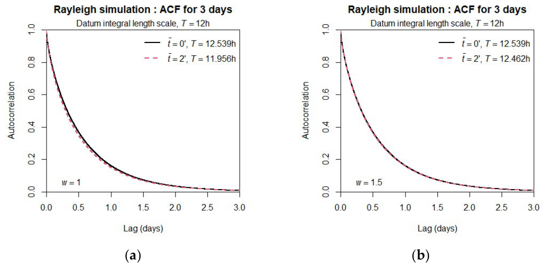
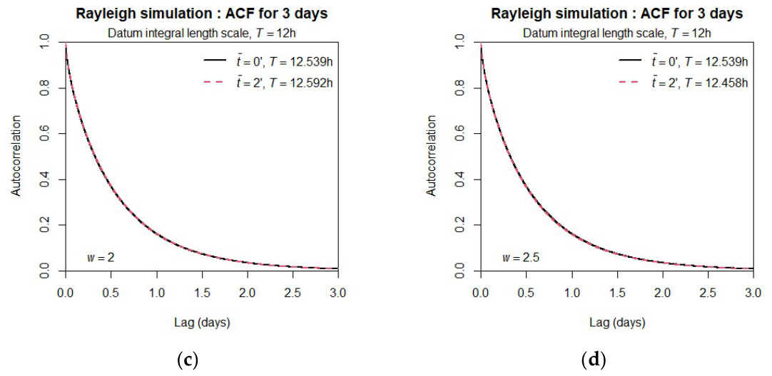
Sensitivity of autocorrelation to Weibull index, w. The solid black curves are the target vK autocorrelations and the dashed red curves are the simulated values. (a) . (b) .5. (c) . (d) .
Figure A1.
Sensitivity of autocorrelation to Weibull index, w. The solid black curves are the target vK autocorrelations and the dashed red curves are the simulated values. (a) . (b) .5. (c) . (d) .
A.1. Autocorrelations
The sensitivity of the autocorrelation was tested by transforming the simulated 2-minute mean wind speeds for the target timescale, h to a range of index values by: , then recomputing the autocorrelation and . The results in Figure A1 indicate that the differences in the autocorrelation are very small and only distinguishable from the target in (a) for . Accordingly, the corresponding variation in is also very small. This indicates that the more complicated Harris simulation method for a general index [36] may not be necessary in practice.
A.2. XIMIS
Sensitivity to the XIMIS preconditioning index was tested by refitting the , h simulation of normalized wind speed extremes over the same range of . The results in Table A1 confirm the long-known trend of wind speed decreasing with increasing [34]. The value corresponding to the mean ASOS index (highlighted in bold), w=1.7, is 1.5% higher than for the datum value of the simulation and the value by the standard Gumbel analysis [29] is ~6% higher.

Table A1.
Sensitivity of the normalized 50-year return 10-minute mean wind speed, , to the XIMIS preconditioning index, .
Table A1.
Sensitivity of the normalized 50-year return 10-minute mean wind speed, , to the XIMIS preconditioning index, .
| 1 | 1.5 | 1.7 | 2 | 2.5 | |
| 12.20±0.47 | 11.70±0.42 | 11.64±0.40 | 11.47±0.38 | 11.22±0.35 |
References
- Kasperski, M. A New Wind Zone Map of Germany. J. Wind Eng. Ind. Aerodyn. 2002, 90, 1271–1287. [Google Scholar] [CrossRef]
- Raffaele, L.; Bruno, L.; Colucci, E. Reanalysis-Based Mesoscale Wind Maps for the Design of Structures and Infrastructures with an Application to Italy. J. Wind Eng. Ind. Aerodyn. 2024, 253, 105844. [Google Scholar] [CrossRef]
- Miller, C. A Once in 50-Year Wind Speed Map for Europe Derived from Mean Sea Level Pressure Measurements. J. Wind Eng. Ind. Aerodyn. 2003, 91, 1813–1826. [Google Scholar] [CrossRef]
- BSI Code of Basic Data for the Design of Buildings, CP3 ChV, Loading, Part 2 Wind Loads; British Standards Institute: Milton Keynes, 1970.
- Cook, N.J. Detecting Artefacts in Analyses of Extreme Wind Speeds. Wind Struct. 2014, 19, 271–294. [Google Scholar] [CrossRef]
- Deaves, D.M. Computations of Wind Flow over Changes in Surface Roughness. J. Wind Eng. Ind. Aerodyn. 1981, 7, 65–94. [Google Scholar] [CrossRef]
- BSI Loading for Buildings. Pt.2 Code of Practice for Wind Loads, BS6399 Pt2; British Standards Institute: Milton Keynes, 1995; ISBN 978-0-580-23651-8.
- CEN Eurocode 1: Actions on Structures - Part 1-4: General Actions - Wind Actions. EN 1991-1-4:2005; European Committee for Standardization: Brussels, 2005.
- Ballio, G.; Lagomarsino, S.; Piccardo, G.; Solari, G. Probabilistic Analysis of Italian Extreme Winds : Reference Velocity and Return Criterion. Wind Struct. 1999, 2, 51–68. [Google Scholar] [CrossRef]
- Harris, R.I. XIMIS, a Penultimate Extreme Value Method Suitable for All Types of Wind Climate. J. Wind Eng. Ind. Aerodyn. 2009, 97, 271–286. [Google Scholar] [CrossRef]
- Larsén, X.G.; Mann, J. The Effects of Disjunct Sampling and Averaging Time on Maximum Mean Wind Speeds. J. Wind Eng. Ind. Aerodyn. 2006, 94, 581–602. [Google Scholar] [CrossRef]
- Chiodi, R.; Ricciardelli, F. Three Issues Concerning the Statistics of Mean and Extreme Wind Speeds. J. Wind Eng. Ind. Aerodyn. 2014, 125, 156–167. [Google Scholar] [CrossRef]
- Cook, N.J. Reliability of Extreme Wind Speeds Predicted by Extreme-Value Analysis. Meteorology 2023, 2, 344–367. [Google Scholar] [CrossRef]
- Gibbons, M.; Sifton, V.; Kilpatrick, J.; Hussain, S. McNamara K Effect of Selective Sampling of Wind Speeds on Parent and Extreme Distributions; Porto Alegre, Brazil, 2015. [Google Scholar]
- Cook, N.J. Curating the TD6405 Database of 1-Min Interval Wind Observations across the USA for Use in Wind Engineering Studies. J. Wind Eng. Ind. Aerodyn. 2022, 224, 104961. [Google Scholar] [CrossRef]
- Si Han Li Effect of Disjunct Sampling on Calibration of Design Wind Speed. JWEIA 2018, 183, 283–294. [CrossRef]
- Nichols, J.M.; Olson, C.C.; Michalowicz, J.V.; Bucholtz, F. A Simple Algorithm for Generating Spectrally Colored, Non-Gaussian Signals. Probabilistic Eng. Mech. 2010, 25, 315–322. [Google Scholar] [CrossRef]
- Picozzi, V.; Akbaba, A.; Avossa, A.M.; Ricciardelli, F. Correction of Historical Records to Improve the Reliability of Design Wind Speeds. Eng. Struct. 2022, 265, 114473. [Google Scholar] [CrossRef]
- Harris, R.I.; Cook, N.J. The Parent Wind Speed Distribution: Why Weibull? J. Wind Eng. Ind. Aerodyn. 2014, 131, 72–87. [Google Scholar] [CrossRef]
- Oort, A.H.; Taylor, A. ON THE KINETIC ENERGY SPECTRUM NEAR THE GROUND. Mon. Wea. Rev. 1969, 97, 623–636. [Google Scholar] [CrossRef]
- Cook, N.J. A Statistical Model of the Seasonal-Diurnal Wind Climate at Adelaide. Aust. Meteorol. Oceanogr. J. 2015, 65, 206–232. [Google Scholar] [CrossRef]
- Cook, N.J. Parameterizing the Seasonal–Diurnal Wind Climate of Rome: Fiumicino and Ciampino. Meteorol. Appl. 2020, 27. [Google Scholar] [CrossRef]
- Cook, N.J. Implications of the OEN Mixture Model of the Mean Wind Vector for the Generation of Synthetic Timeseries and for the Assessment of Extremes. J. Wind Eng. Ind. Aerodyn. 2021, 208, 104424. [Google Scholar] [CrossRef]
- Lombardo, F.T.; Zickar, A.S. Characteristics of Measured Extreme Thunderstorm Near-Surface Wind Gusts in the United States. J. Wind Eng. Ind. Aerodyn. 2019, 193, 103961. [Google Scholar] [CrossRef]
- Vickery, P.J.; Masters, F.J.; Powell, M.D.; Wadhera, D. Hurricane Hazard Modeling: The Past, Present, and Future. J. Wind Eng. Ind. Aerodyn. 2009, 97, 392–405. [Google Scholar] [CrossRef]
- Priestley, M.D.K.; Stephenson, D.B.; Scaife, A.A.; Bannister, D.; Allen, C.J.T.; Wilkie, D. Return Levels of Extreme European Windstorms, Their Dependency on the NAO, and Potential Future Risks; Atmospheric, Meteorological and Climatological Hazards, 2023 .
- Cook, N.J. Automated Classification of Gust Events in the Contiguous USA. J. Wind Eng. Ind. Aerodyn. 2023, 234, 105330. [Google Scholar] [CrossRef]
- Harris, R.I. The Macrometeorological Spectrum—a Preliminary Study. J. Wind Eng. Ind. Aerodyn. 2008, 96, 2294–2307. [Google Scholar] [CrossRef]
- Gumbel, E.J. Statistics of Extremes; Columbia Univ. Press: New York, NY, 1958; ISBN 978-0-231-02190-6. [Google Scholar]
- Takle, E.S.; Brown, J.M. Note on the Use of Weibull Statistics to Characterize Wind-Speed Data. J. Appl. Meteor. 1978, 17, 556–559. [Google Scholar] [CrossRef] [PubMed]
- Davenport, A.G. Note on the Distribution of the Largest Value of a Random Function with Application to Gust Loading. Proc. Inst. Civ. Eng. 1964, 28, 187–196. [Google Scholar] [CrossRef]
- Rice, S.O. Mathematical Analysis of Random Noise. Bell Syst. Tech. J. 1944, 23, 282–332. [Google Scholar] [CrossRef]
- Cook, N.J. On Extracting Independent Peak Values from Correlated Time Series for Assessing Extremes. J. Wind Eng. Ind. Aerodyn. 2017, 170, 274–282. [Google Scholar] [CrossRef]
- Cook, N.J. Towards Better Estimation of Extreme Winds. J. Wind Eng. Ind. Aerodyn. 1982, 9, 295–323. [Google Scholar] [CrossRef]
- Harris, R.I. A Simulation Method for the Macro-Meteorological Wind Speed and the Implications for Extreme Value Analysis. J. Wind Eng. Ind. Aerodyn. 2014, 125, 146–155. [Google Scholar] [CrossRef]
- Harris, R.I. A Simulation Method for Macro-Meteorological Wind Speeds with a Forward Weibull Parent Distribution of General Index. J. Wind Eng. Ind. Aerodyn. 2017, 171, 202–206. [Google Scholar] [CrossRef]
- Box, G.E.P.; Jenkins, G.M.; Reinsel, G.C. Time Series Analysis: Forecasting and Control, 3rd ed.; Prentice Hall: Englewood Cliffs (N.J.), 1994; ISBN 978-0-13-060774-4. [Google Scholar]
- van der Hoven, I. Power Spectrum of Horizontal Wind Speed in the Frequency Range from 0.0007 to 900 Cycles per Hour. J. Meteor. 1957, 14, 160–164. [Google Scholar] [CrossRef]
- Cook, N.J. The OEN Mixture Model for the Joint Distribution of Wind Speed and Direction: A Globally Applicable Model with Physical Justification. Energy Convers. Manag. 2019, 191, 141–158. [Google Scholar] [CrossRef]
- ASCE Minimum Design Loads and Associated Criteria for Buildings and Other Structures, ASCE 7-22; American Society of Civil Engineers: Reston, 2021; ISBN 978-0-7844-8349-7.
- Cook, N.J. Extreme Convective Gusts in the Contiguous USA. Meteorology 2024, 3, 281–309. [Google Scholar] [CrossRef]
- Torrielli, A.; Repetto, M.P.; Solari, G. The Annual Rate of Independent Events – A Key Interpretation for Traditional Extreme Value Distributions of Wind Velocity. Wind Energy 2022, 25, 1188–1202. [Google Scholar] [CrossRef]
- Harris, R.I. Discussion of “The Annual Rate of Independent Events for the Analysis of Extreme Wind Speed” By Alessio Torrielli, Maria Pia Repetto & Giovanni Solari. J. Wind Eng. Ind. Aerodyn. 2017, 164, 174–178. [Google Scholar] [CrossRef]
- Torrielli, A.; Repetto, M.P.; Solari, G. Response to the Further Discussion on “The Annual Rate of Independent Events for the Analysis of Extreme Wind Speed, by N. Cook.”. J. Wind Eng. Ind. Aerodyn. 2018, 174, 464–465. [Google Scholar] [CrossRef]
- Gomes, L.; Vickery, B.J. Extreme Wind Speeds in Mixed Wind Climates. J. Wind Eng. Ind. Aerodyn. 1978, 2, 331–344. [Google Scholar] [CrossRef]
- Cook, N.J.; Harris, R.I.; Whiting, R. Extreme Wind Speeds in Mixed Climates Revisited. J. Wind Eng. Ind. Aerodyn. 2003, 91, 403–422. [Google Scholar] [CrossRef]
- Beck, H.E.; McVicar, T.R.; Vergopolan, N.; Berg, A.; Lutsko, N.J.; Dufour, A.; Zeng, Z.; Jiang, X.; Van Dijk, A.I.J.M.; Miralles, D.G. High-Resolution (1 Km) Köppen-Geiger Maps for 1901–2099 Based on Constrained CMIP6 Projections. Sci. Data 2023, 10, 724. [Google Scholar] [CrossRef] [PubMed]
- Arul, M.; Kareem, A.; Burlando, M.; Solari, G. Machine Learning Based Automated Identification of Thunderstorms from Anemometric Records Using Shapelet Transform. J. Wind Eng. Ind. Aerodyn. 2022, 220, 104856. [Google Scholar] [CrossRef]
Figure 1.
Continuous, contiguous and disjoint sampling at KSLN – Salina, KS, over the 5h period centered on the maximum recorded mean between 2000 and 2023. (a) 10-minute mean wind speeds, . (b) Hourly-mean wind speeds, .
Figure 1.
Continuous, contiguous and disjoint sampling at KSLN – Salina, KS, over the 5h period centered on the maximum recorded mean between 2000 and 2023. (a) 10-minute mean wind speeds, . (b) Hourly-mean wind speeds, .
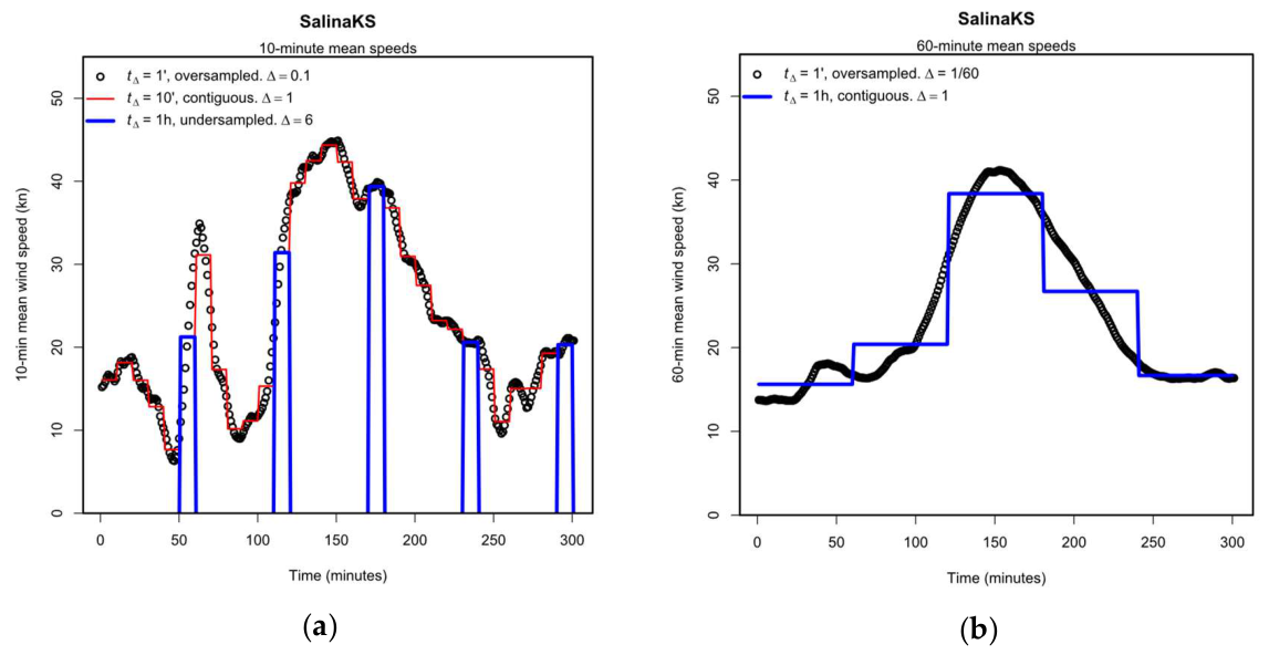
Figure 2.
Locations of WMO exposure category 1 and 2 ASOS stations across CONUS used in this study. The background color scale indicates the geographical density in stations per 1° square.
Figure 2.
Locations of WMO exposure category 1 and 2 ASOS stations across CONUS used in this study. The background color scale indicates the geographical density in stations per 1° square.
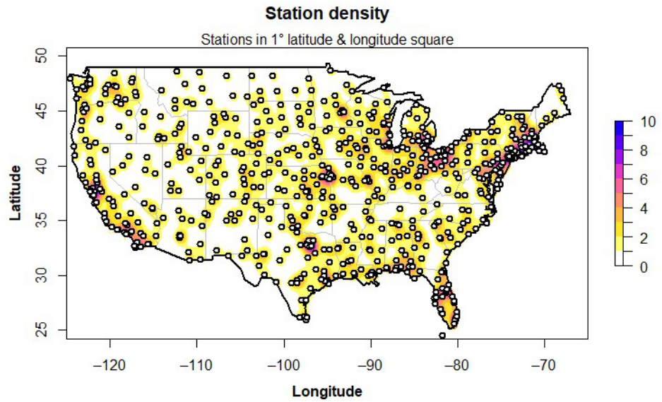
Figure 3.
Example autocovariance for KBOS, Boston MA. (a) Observed, first 10 days. (b) Observed, full 2 years. (c) Synoptic component after heterodyning.
Figure 3.
Example autocovariance for KBOS, Boston MA. (a) Observed, first 10 days. (b) Observed, full 2 years. (c) Synoptic component after heterodyning.
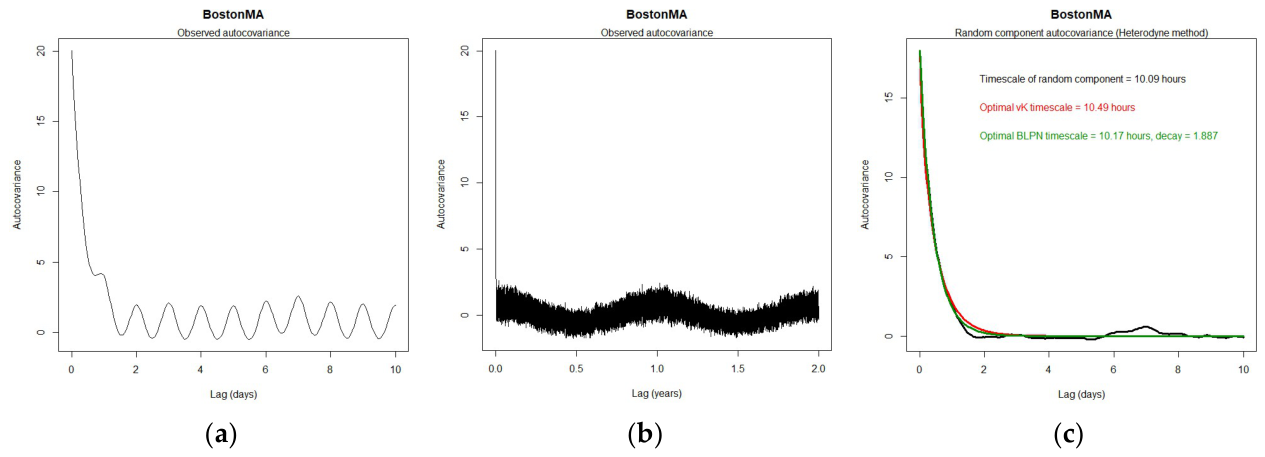
Figure 4.
Weibull analysis of time-averaged wind speed at KBOS, Boston, MA. (a) Weibull plot for . (b) PDF of for , and .
Figure 4.
Weibull analysis of time-averaged wind speed at KBOS, Boston, MA. (a) Weibull plot for . (b) PDF of for , and .
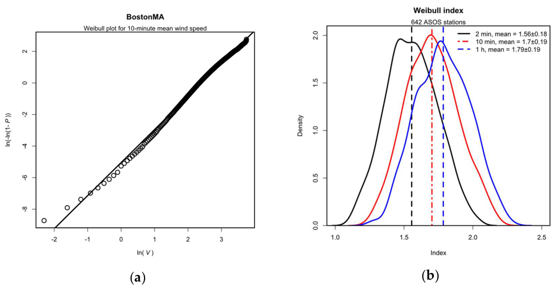
Figure 5.
Locating peaks between up/down-crossings of the mean using the averaged wind speed. (a) KBOS, Boston, MA. (b) Rayleigh simulation.
Figure 5.
Locating peaks between up/down-crossings of the mean using the averaged wind speed. (a) KBOS, Boston, MA. (b) Rayleigh simulation.
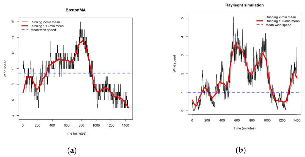
Figure 6.
XIMIS analysis for average wind speeds at KBOS, Boston, MA. (a) . (b) . (c) . Key: + subset peaks; ◯ ensemble peaks; central thick curve – fit to ensemble; chained curves – 5%-95% confidence limits for subset peaks; thin (red) curves – 5%-95% confidence limits for fit.
Figure 6.
XIMIS analysis for average wind speeds at KBOS, Boston, MA. (a) . (b) . (c) . Key: + subset peaks; ◯ ensemble peaks; central thick curve – fit to ensemble; chained curves – 5%-95% confidence limits for subset peaks; thin (red) curves – 5%-95% confidence limits for fit.
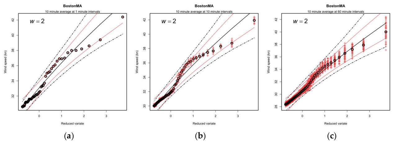
Figure 7.
ASOS stations. Geographical variation of autocorrelation. (a) Distribution of vK integral timescale, (h). (b) Distribution of BLPN integral timescale, (h). (c) Difference of timescales of vK from BLPN (%). (d) BLPN decay index.
Figure 7.
ASOS stations. Geographical variation of autocorrelation. (a) Distribution of vK integral timescale, (h). (b) Distribution of BLPN integral timescale, (h). (c) Difference of timescales of vK from BLPN (%). (d) BLPN decay index.
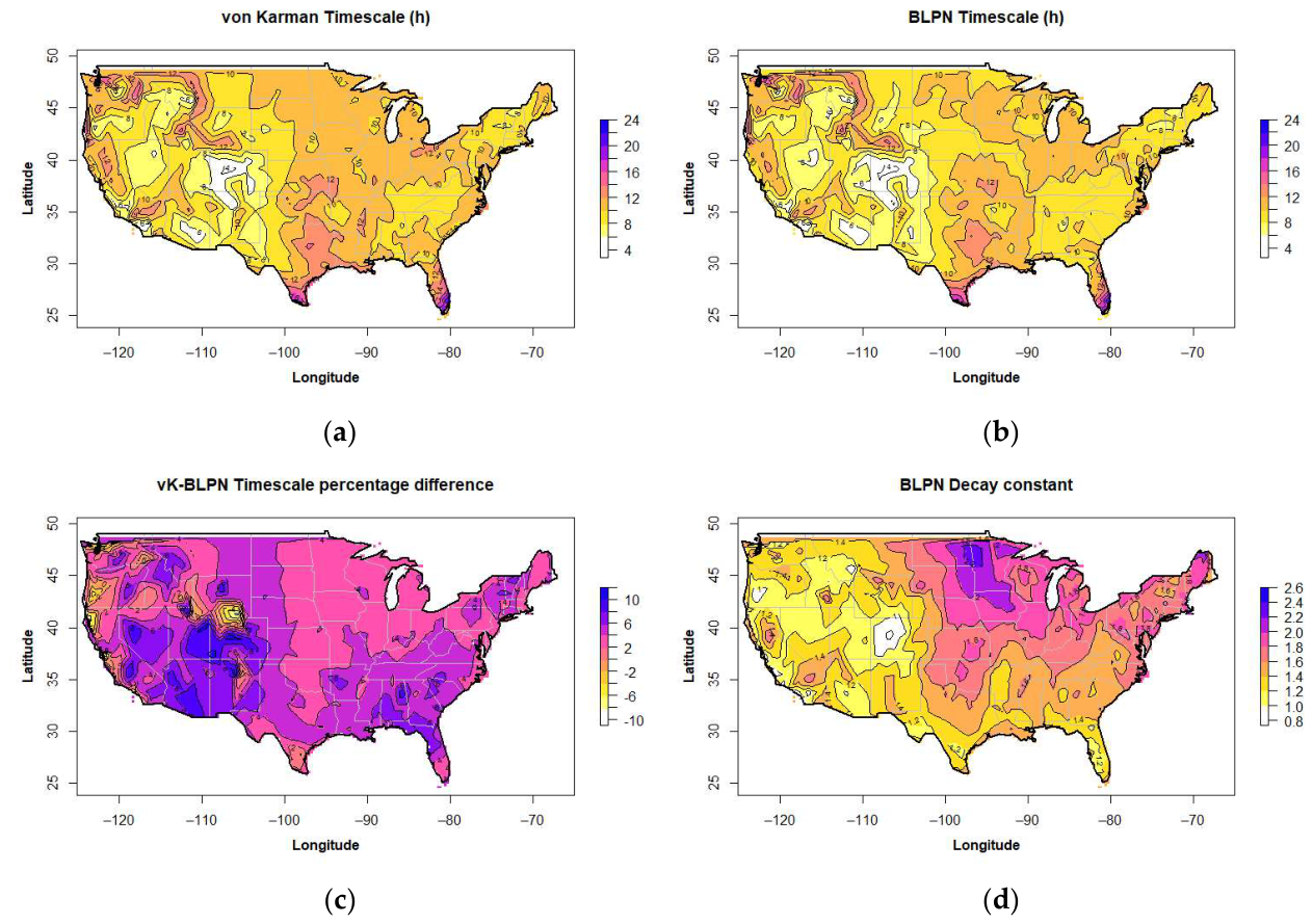
Figure 8.
ASOS stations, BLPN model decay index. (a) PDF of decay index, east/west of longitude −100°. (b) Q-Q plot of integral timescale and decay index.
Figure 8.
ASOS stations, BLPN model decay index. (a) PDF of decay index, east/west of longitude −100°. (b) Q-Q plot of integral timescale and decay index.
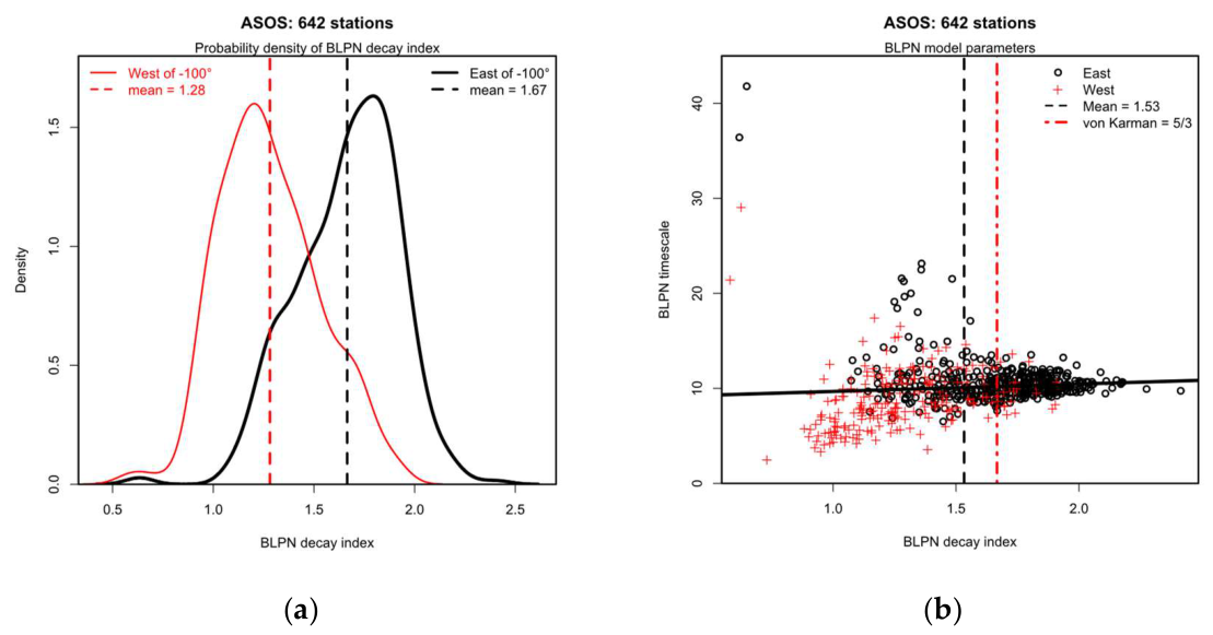
Figure 9.
ASOS stations. Geographical distribution and standard error of the Weibull index. (a) Distribution of Weibull index, . (b) Q-Q plot for with 5%/95% confidence limits (dashed lines).
Figure 9.
ASOS stations. Geographical distribution and standard error of the Weibull index. (a) Distribution of Weibull index, . (b) Q-Q plot for with 5%/95% confidence limits (dashed lines).
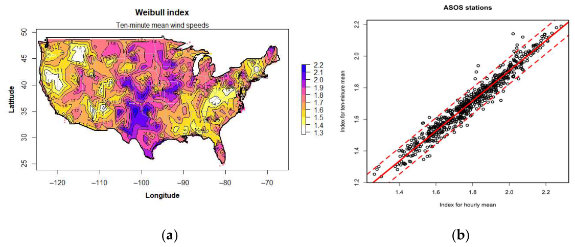
Figure 10.
ASOS stations. Q-Q plots of 50y-return mean wind speed,
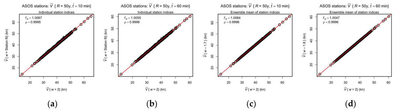
Figure 11.
ASOS stations. 50-year return mean wind speed from 1-minute interval observations. (a) 10-minute average wind speed (kn). (b) Hourly average wind speed (kn).
Figure 11.
ASOS stations. 50-year return mean wind speed from 1-minute interval observations. (a) 10-minute average wind speed (kn). (b) Hourly average wind speed (kn).
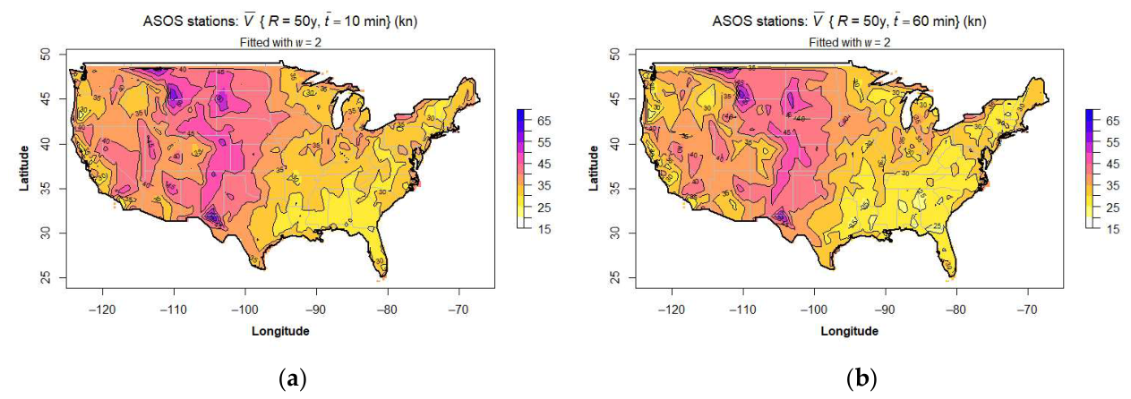
Figure 12.
Sampling transformation factors, , to 1-minute intervals. (a) Annual maxima, . (b) 50-year return period, . (c) 1000-year return period,
Figure 12.
Sampling transformation factors, , to 1-minute intervals. (a) Annual maxima, . (b) 50-year return period, . (c) 1000-year return period,
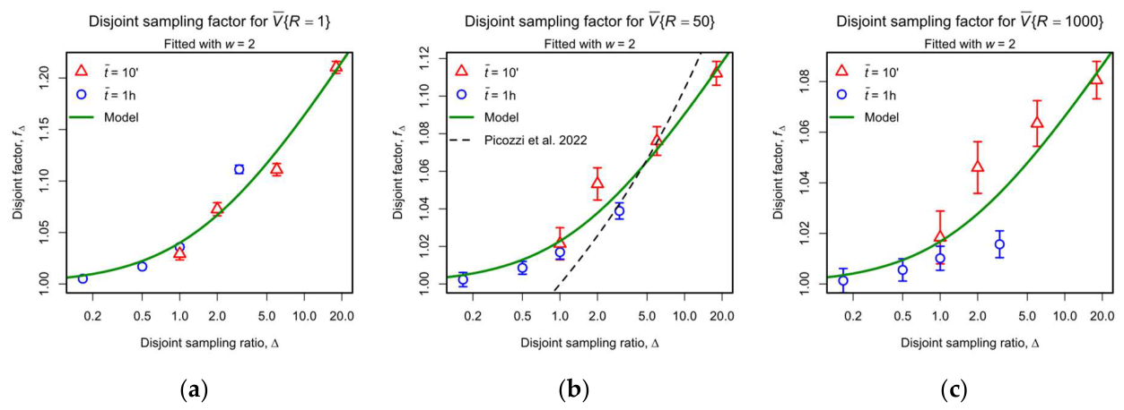
Figure 13.
ASOS stations, sampling transformation factor, for . (a) All ASOS stations. (b) ASOS stations within 5%−95% confidence limits.
Figure 13.
ASOS stations, sampling transformation factor, for . (a) All ASOS stations. (b) ASOS stations within 5%−95% confidence limits.
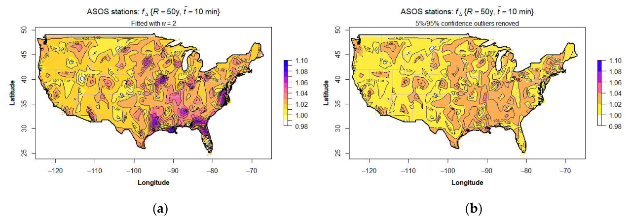
Figure 14.
ASOS stations. Averaging period transformation factor, , for . (a) All ASOS stations. (b) ASOS stations within 5%−95% confidence limits.
Figure 14.
ASOS stations. Averaging period transformation factor, , for . (a) All ASOS stations. (b) ASOS stations within 5%−95% confidence limits.
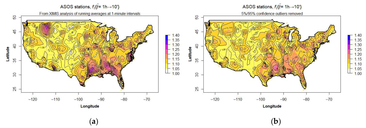
Figure 15.
Rayleigh simulations: example autocorrelations and integral time scales. (a) ACF near the origin for target . (b) ACF for target . (c) ACF for target . The key in (b,c) includes the values of achieved for each simulation.
Figure 15.
Rayleigh simulations: example autocorrelations and integral time scales. (a) ACF near the origin for target . (b) ACF for target . (c) ACF for target . The key in (b,c) includes the values of achieved for each simulation.
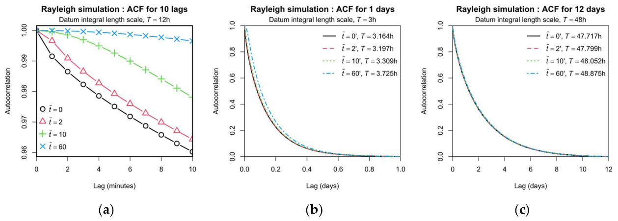
Figure 16.
Disjoint sampling factor, . (a) Smallest . (b) Typical . (c) Largest .
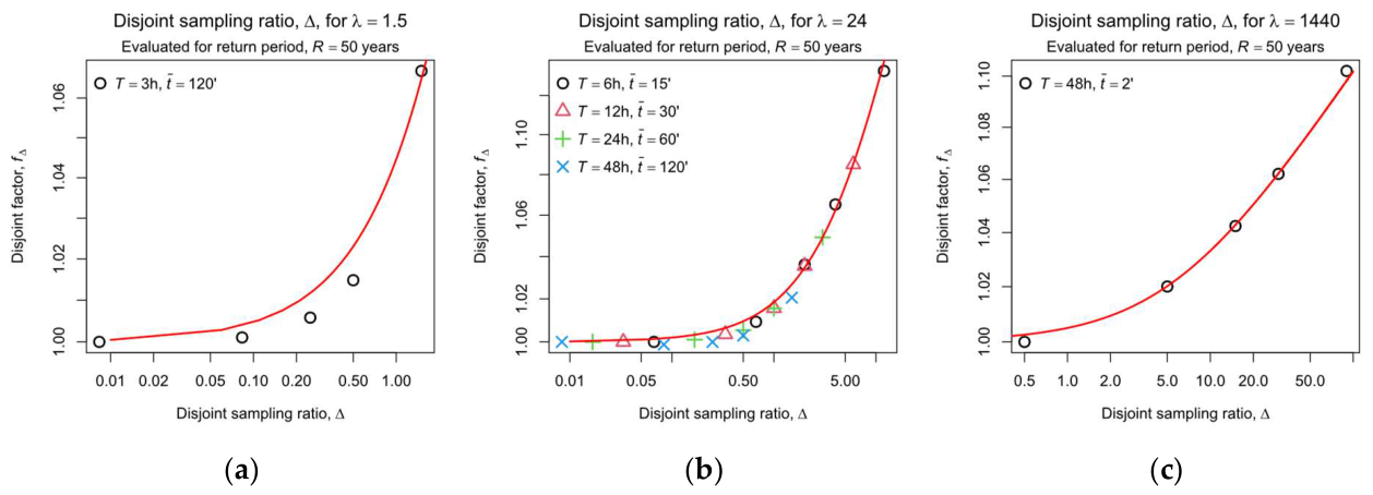
Figure 17.
Rayleigh model for coefficient in Equation (6) for and
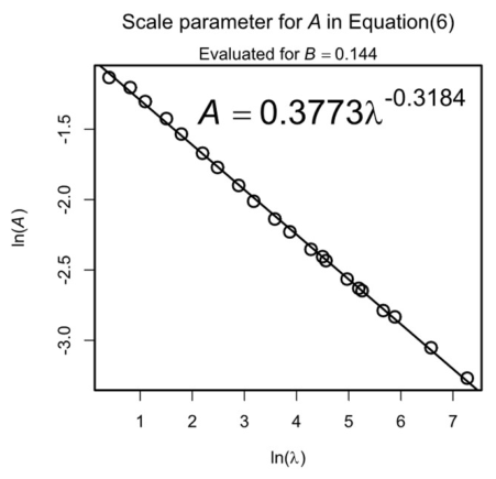
Figure 18.
Rayleigh model for the disjoint sampling factor, . See text for key to annotations A to H.
Figure 18.
Rayleigh model for the disjoint sampling factor, . See text for key to annotations A to H.
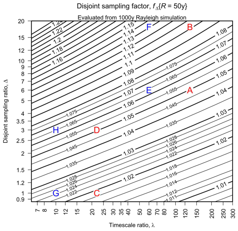
Figure 19.
Dependence of Rayleigh disjoint sampling factor . on return period. (a) Excess over unity, . (b). Adjustment factor, C, for .
Figure 19.
Dependence of Rayleigh disjoint sampling factor . on return period. (a) Excess over unity, . (b). Adjustment factor, C, for .
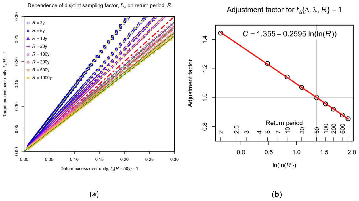
Figure 20.
Fidelity of Equation (10) for .
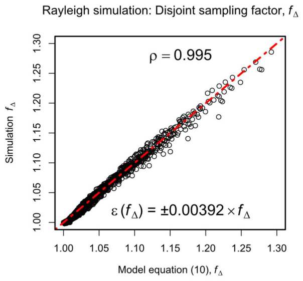
Figure 21.
Dependence of averaging period factor, , on sampling interval, , and integral timescale, , at the datum return period, .
Figure 21.
Dependence of averaging period factor, , on sampling interval, , and integral timescale, , at the datum return period, .
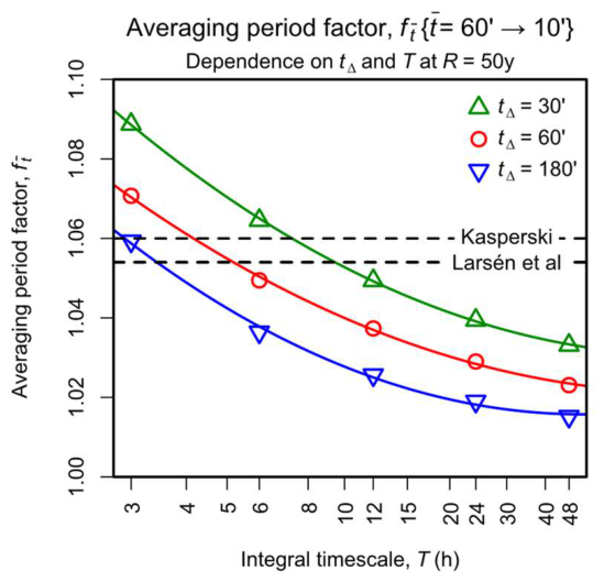
Figure 22.
Major Köppen-Geiger climate classes for CONUS, sourced from [47].
Figure 22.
Major Köppen-Geiger climate classes for CONUS, sourced from [47].
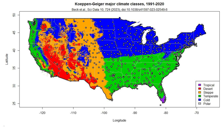
Figure 23.
ASOS sampling interval factor, , for compared with Rayleigh model predictions. (a) All stations. (b) Western stations. (c) Northeastern stations. (d) Southeastern stations.
Figure 23.
ASOS sampling interval factor, , for compared with Rayleigh model predictions. (a) All stations. (b) Western stations. (c) Northeastern stations. (d) Southeastern stations.
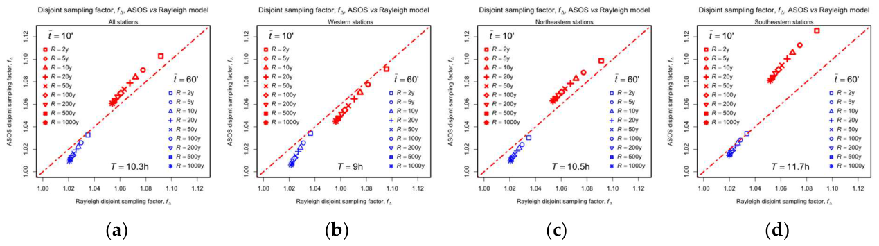
Figure 24.
ASOS sampling interval factor, , for and with optimised for ten-minute means. (a) All stations. (b) Western stations. (c) Northeastern stations. (d) Southeastern stations.
Figure 24.
ASOS sampling interval factor, , for and with optimised for ten-minute means. (a) All stations. (b) Western stations. (c) Northeastern stations. (d) Southeastern stations.
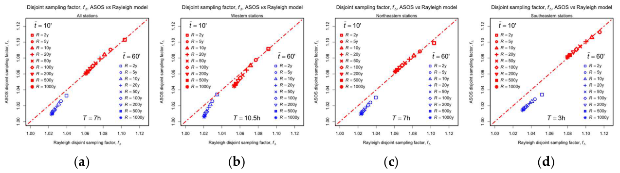
Table 1.
Factors for from previous studies.
| Study | Factor | ||
| [9] | 18 | 1.05 – 1.10 | |
| [1] | 1 | 1.06 | |
| [11] |
|
1 6 18 |
1.054 1.031 1.06 |
| [12] |
|
3 6 18 |
1.03 1.05 1.08 |
| [16] | 6 | 1.04 | |
| [18] |
|
6 18 |
1.076 1.142 |
Table 2.
ASOS: Disjoint sampling factors, , to 1-minute sample intervals for years.
| Observed | ||||
| Station w | 1.021±0.0169 | 1.052±0.0294 | 1.074±0.0368 | 1.105±0.0533 |
| Mean w | 1.021±0.0169 | 1.052±0.0293 | 1.074±0.0369 | 1.106±0.0531 |
| Rayleigh w | 1.021±0.0164 | 1.053±0.0286 | 1.076±0.0359 | 1.112±0.0516 |
| (b) 1. hour mean wind speeds. | ||||
| Observed | ||||
| Station w | 1.002±0.00744 | 1.008±0.0118 | 1.016±0.0182 | 1.035±0.0365 |
| Mean w | 1.002±0.00741 | 1.008±0.0117 | 1.016±0.0181 | 1.036±0.0362 |
| Rayleigh w | 1.002±0.00723 | 1.009±0.0114 | 1.017±0.0176 | 1.039±0.0352 |
Table 3.
Coefficients in Equation (6) for
| A | B | |
| R = 1 year | 0.08329 | 0.6617 |
| R = 50 years | 0.04397 | 0.6820 |
| R = 1000 years | 0.03215 | 0.6857 |
Table 4.
First-order adjustment factors to from to truly continuous, .
| R = 1 year | 1.00499 | 1.00085 |
| R = 50 years | 1.00290 | 1.00050 |
| R = 1000 years | 1.00213 | 1.00037 |
Table 5.
Averaging factor for averaging period, , from the running average wind speed over threshold.
Table 5.
Averaging factor for averaging period, , from the running average wind speed over threshold.
| Threshold (kn) | |||
| 10 | 1.02±0.011 | 1.06±0.023 | 1.03±0.013 |
| 20 | 1.03±0.017 | 1.08±0.039 | 1.04±0.021 |
| 30 | 1.04±0.020 | 1.10±0.057 | 1.06±0.032 |
| 40 | 1.06±0.018 | 1.13±0.064 | 1.07±0.036 |
| 50 | 1.07±0.017 | 1.18±0.071 | 1.10±0.048 |
| 60 | 1.10±0.050 | 1.25±0.137 | 1.13±0.060 |
Table 6.
Rayleigh simulations: integral timescales, (h).
| Target | ||||
| 3.16 | 3.20 | 3.31 | 3.72 | |
| 6.32 | 6.36 | 6.50 | 6.98 | |
| 12.54 | 12.59 | 12.76 | 13.33 | |
| 24.84 | 24.91 | 25.12 | 25.81 | |
| 47.72 | 47.80 | 48.05 | 48.88 |
Table 7.
Rayleigh simulation: Ensemble averaged 50-year return, contiguous 10-minute average wind speed (kn).
Table 7.
Rayleigh simulation: Ensemble averaged 50-year return, contiguous 10-minute average wind speed (kn).
| 12.865 | 12.555 | 12.072 | 11.592 | 11.062 | |
| 12.860 | 12.546 | 12.069 | 11.593 | 11.059 | |
| 12.860 | 12.542 | 12.068 | 11.593 | 11.059 | |
| 12.859 | 12.541 | 12.068 | 11.595 | 11.059 |
Table 8.
Coefficients in Equation (11) evaluated for
| D | E | F | |
| 1.9659 | -0.8529 | 0.1945 | |
| 1.8142 | -0.7231 | 0.1648 | |
| 1.9770 | -0.9205 | 0.2203 |
Table 9.
Evaluations of
| Derivation | |||||
| Simulation | 1.071 | 1.050 | 1.037 | 1.029 | 1.023 |
| Equation (11) | 1.070 | 1.050 | 1.037 | 1.028 | 1.023 |
| Equation (12) | 1.056 | 1.045 | 1.036 | 1.029 | 1.024 |
Table 10.
Evaluations of for transforming contiguous hourly-means to continuous -means.
| 1.091 | 1.073 | 1.058 | 1.047 | 1.037 | |
| 1.155 | 1.124 | 1.099 | 1.079 | 1.063 | |
| 1.298 | 1.237 | 1.190 | 1.152 | 1.121 |
| 1 | |
| 2 | |
| 3 |
Disclaimer/Publisher’s Note: The statements, opinions and data contained in all publications are solely those of the individual author(s) and contributor(s) and not of MDPI and/or the editor(s). MDPI and/or the editor(s) disclaim responsibility for any injury to people or property resulting from any ideas, methods, instructions or products referred to in the content. |
© 2026 by the author. Licensee MDPI, Basel, Switzerland. This article is an open access article distributed under the terms and conditions of the Creative Commons Attribution (CC BY) license.
Copyright: This open access article is published under a Creative Commons CC BY 4.0 license, which permit the free download, distribution, and reuse, provided that the author and preprint are cited in any reuse.


