
Submitted:
22 July 2026
Posted:
22 July 2026
You are already at the latest version
Abstract
Submarine telecommunication cables carry over 99% of international data traffic yet remain persistently vulnerable to geophysical, anthropogenic, and oceanographic hazards. Existing risk assessment methods , GIS-based least-cost path analysis and cable-body condition monitoring , operate in isolation, cannot fuse heterogeneous multi-modal data, and yield neither uncertainty estimates nor physics-consistent predictions. We present MarineGuard-GNN, a physics-informed multimodal heterogeneous graph neural network that unifies four hazard modalities , bathymetric, oceanographic, vessel traffic, and seismic , in a single relational graph over four semantic node types and four typed relation edges. Three novel technical contributions distinguish the framework: (i) the Cross-Modal Spatiotemporal Tokenizer (CMST), which jointly encodes GEBCO bathymetric raster fields via a SatMAE-pretrained ViT-S and NOAA AIS vessel trajectories via a Transformer-XL into a unified 256-dimensional token space, addressing the modality-heterogeneity gap; (ii) a Physics-Informed Heterogeneous Graph Transformer with a differentiable Mohr–Coulomb geomechanical shear-stress regularization loss Lphys that prevents physically inconsistent risk assignments at steep bathymetric gradients; and (iii) a Bayesian Uncertainty-Aware Risk Head using Monte Carlo Dropout (K=50, p=0.3) to produce calibrated epistemic uncertainty maps for inspection prioritization. Under strict 4-fold geographic cross-validation across the Pacific, Atlantic, Indian, and Mediterranean basins using five publicly available datasets, MarineGuard-GNN achieves the highest mean AUC-ROC (0.7228±0.0665) and Average Precision (0.6418±0.1040) among five baselines. A Dijkstra-based spatial route optimizer reduces mean predicted fault risk by 0.0035 absolute on the Atlantic New York–UK corridor, avoiding one additional high-risk node at a distance overhead of only +7.4 km (+0.56%). All code, preprocessing pipelines, and datasets are publicly available.
Keywords:
submarine cable
; heterogeneous graph neural network
; physics-informed machine learning
; multimodal remote sensing
; fault risk assessment
; Mohr Coulomb criterion
; Bayesian uncertainty quantification
; vessel AIS data
; subsea route optimization
1. Introduction
Submarine telecommunication cables constitute the physical nervous system of the global internet, carrying over 99% of international data traffic across approximately 1.4 million kilometres of seabed-laid optical fibre (Carter & Burnett, 2009). More than 400 active cable systems interconnect every inhabited continent, supporting an estimated $10 trillion in daily financial transactions and underpinning critical services ranging from cloud computing to military communications (Insikt Group, 2025). Despite their infrastructural centrality, these systems are persistently vulnerable: the International Cable Protection Committee (ICPC) recorded 46 fault events in 2024 alone , the highest annual total since systematic reporting began in 2013 (Lapa & Vieira, 2024) , with individual repair operations costing $1–3 million and requiring weeks to months of service disruption. Submarine cable faults arise from three primary causal pathways (Figure 1): anthropogenic hazards (vessel anchoring and bottom trawling, accounting for approximately 48% of shallow-water faults), seismic and geohazard events (earthquake-triggered turbidity currents and submarine landslides, as demonstrated by the 2006 Pingtung earthquake that severed approximately 20 cables across Southeast Asia (Lapa & Vieira, 2024)), and oceanographic forcing (near-bed current scour, sediment mobilization, and thermally-driven geomechanical stress). These hazard pathways are spatially heterogeneous, temporally dynamic, and mutually interacting , a combination that fundamentally limits the effectiveness of conventional risk assessment methods based on static geospatial overlays or tabular hazard scores.
Existing approaches to submarine cable risk assessment fall into two broad categories, neither of which is adequate for operational risk intelligence. GIS-based least-cost path analysis (LCPA) methods (Deligiannidis & Kkanas, 2023; Furlong, 2026) select cable routes by minimizing weighted combinations of bathymetric slope, sediment class, and fault zone proximity, but produce deterministic risk scores that cannot capture relational hazard interactions, adapt to dynamic oceanographic and vessel-traffic data, or provide the calibrated uncertainty estimates required for data-sparse oceanic regions. Condition monitoring approaches (Carr & Allanic, 2023) detect physical cable degradation from acoustic or electrical sensor data at the cable-body level but cannot anticipate fault risk from environmental precursors, addressing only approximately 30% of known failure mechanisms. Graph neural networks (GNNs) have emerged as the natural framework for multi-relational spatial risk reasoning (Carter & Burnett, 2009; Mao & Cao, 2023; Varbella & Tanneau, 2024; Taghizadeh & Bentivoglio, 2025; Sarkar & Hakimi, 2025), yet existing GNN risk frameworks share three limitations that preclude direct application to submarine cable fault prediction. First, modality homogeneity: existing frameworks operate on a single data type and cannot fuse raster satellite imagery with irregular vessel trajectory sequences. Second, physics-agnosticism: they impose no geomechanical constraints on predicted risk values, permitting physically inconsistent predictions at steep bathymetric gradients under cross-basin distribution shift. Third, deterministic inference: they produce point estimates without epistemic uncertainty quantification, preventing safety-critical deployment in data-sparse oceanic regions where model confidence is lowest and inspection stakes are highest.
To address these three limitations simultaneously, we propose MarineGuard-GNN (Figure 2) , a physics-informed multimodal heterogeneous graph neural network that represents the cable network as a heterogeneous spatial graph with four semantic node types (cable, vessel, seismic, ocean) and four typed relation edges encoding spatial adjacency, vessel route intersection, oceanographic forcing, and seismic proximity. The Cross-Modal Spatiotemporal Tokenizer (CMST) resolves the modality heterogeneity problem by jointly encoding GEBCO 2023 bathymetric and CMEMS oceanographic raster fields through a SatMAE-pretrained ViT-S patch encoder and NOAA AIS vessel mobility sequences through a Transformer-XL trajectory encoder, fusing both into a unified -dimensional node feature space via geodesic proximity-weighted cross-attention grounded on cable-segment positions; ablation analysis confirms that removing the CMST increases mean absolute error by 27.9% (MAE from 0.4577 to 0.5856 on the Atlantic fold), confirming its role in calibrating absolute risk magnitudes. The Physics-Informed HGT with Mohr–Coulomb Constraint stacks three Heterogeneous Graph Transformer (HGT) layers (Hu & Dong, 2020) with relation-type-aware attention, jointly trained with a differentiable Mohr–Coulomb geomechanical shear-stress penalty that prevents physically inconsistent risk assignments at geomechanically stable segments, with the Pacific fold achieving the highest per-fold AUC-ROC of 0.7823, consistent with the physics regularizer’s greatest benefit in data-sparse training conditions. The Bayesian Uncertainty-Aware Risk Head employs Monte Carlo Dropout ( forward passes, ) (Song & Alam, 2026) to produce calibrated mean risk predictions , epistemic uncertainty estimates , and 90% confidence intervals for each cable segment, enabling both uncertainty-conditioned inspection prioritization and the exclusion of epistemically uncertain nodes from automated routing decisions. The resulting risk field feeds a Dijkstra-based spatial route optimization framework that, applied to the Atlantic New York–UK corridor, reduces mean predicted fault risk by 0.0035 absolute and avoids one additional high-risk node at a distance penalty of only km ().
The principal contributions of this paper are: (i) a formally specified heterogeneous spatial graph representation integrating four distinct physical hazard modalities into a unified relational structure for submarine cable risk assessment; (ii) the Cross-Modal Spatiotemporal Tokenizer (CMST), the first architecture to jointly encode satellite raster fields and AIS trajectory sequences into a shared token space for cable segment risk representation; (iii) a physics-informed HGT training objective embedding Mohr–Coulomb geomechanical constraints as a differentiable loss term, enabling geophysically consistent risk prediction under cross-basin distribution shift; (iv) a Bayesian uncertainty-aware inference pipeline providing actionable epistemic uncertainty maps for operational cable inspection prioritization and safety-critical route planning; and (v) a risk-optimal route optimization framework demonstrating quantifiable fault risk reduction on the Atlantic corridor, with a fully reproducible open-source implementation on five public datasets. The remainder of this paper is organized as follows. Section 2 reviews related work across five relevant bodies of literature. Section 3 presents the MarineGuard-GNN framework in full technical detail, incorporating the merged problem formulation. Section 4 describes the datasets and preprocessing pipeline. Section 5 reports experimental results under geographic cross-validation, including ablation, calibration, and qualitative analysis. Section 6 presents the route optimization framework and Atlantic corridor results. Section 7 concludes with limitations and future directions.
2. Related Work
2.1. Submarine Cable Risk, Fault Analysis, and Route Planning
Submarine cable systems constitute the physical backbone of global internet connectivity, yet their vulnerability to geophysical, anthropogenic, and oceanographic hazards remains insufficiently characterized in the machine learning literature (Morency & Bhatt, 2026). The most directly related geospatial work applies GIS-based LCPA to submarine cable route selection: Deligiannidis et al. (Deligiannidis & Kkanas, 2023) combined GIS-LCPA with the Analytic Hierarchy Process to optimize cable routes in the seismically active Mediterranean region, incorporating active fault zones, seabed slope, and water depth as multi-criteria routing constraints, but without dynamic oceanographic data or uncertainty quantification. Similarly, recent work on offshore wind export cable optimization (Furlong, 2026) confirms that water depth, slope, and geological hazards are the most consistently cited routing criteria , consistent with the feature design of our cable-segment node representation . On the geohazard side, Lapa et al. (Lapa & Vieira, 2024) integrated a frequency ratio model with supervised machine learning on the South-West Iberian margin to quantify submarine landslide susceptibility, while deep learning segmentation approaches (Li, 2024) have been applied to landslide identification from bathymetric DEM data using slope, hillshade, and elevation features directly comparable to our GEBCO-derived node features. Health monitoring of subsea power cables has been explored by Carr et al. (Carr & Allanic, 2023), who noted that existing approaches address only approximately 30% of cable failure mechanisms , a gap that motivates the environmental-precursor approach of MarineGuard-GNN. The geopolitical dimension of cable risk (Morency & Bhatt, 2026) provides quantitative evidence that route diversity is the primary systemic resilience factor, motivating the route optimization framework in Section 6.
2.2. Graph Neural Networks for Spatial and Infrastructure Risk
GNN architectures used as baselines in our experiments , GCN (ITU IAB Working Groups, 2026), GAT (Velicčković & Cucurull, 2018), and GraphSAGE (Hamilton & Ying, 2017) , were originally designed for homogeneous graphs and do not natively support type-specific message-passing semantics. The Heterogeneous Graph Transformer (HGT) (Hu & Dong, 2020) introduced relation-type-aware attention and demonstrated strong performance on multi-relational node classification tasks; MarineGuard-GNN extends HGT with a physics-informed regularization term and Bayesian inference head. For spatiotemporal infrastructure risk, Shi et al. (Shi & Luo, 2024) demonstrated that explicitly modeling heterogeneous spatial dependencies substantially improves generalization under distribution shift , consistent with our cross-basin evaluation results in Section 5. Mao et al. (Mao & Cao, 2023) established that relational context across infrastructure nodes of different types is essential for accurate vulnerability estimation, directly motivating our four-type heterogeneous graph formulation. For power grids, Varbella et al. (Varbella & Tanneau, 2024) showed that physics-consistent supervision substantially improves temporal extrapolation , an analogue to our Mohr–Coulomb penalty. Taghizadeh et al. (Taghizadeh & Bentivoglio, 2025) demonstrated that physics-informed GNNs achieve superior calibration compared to purely data-driven GNN baselines on out-of-sample hydrological regimes, while HydroGAT (Sarkar & Hakimi, 2025) extended heterogeneous graph attention to spatiotemporal flood prediction with heterogeneous node types structurally similar to ours.
2.3. Physics-Informed Machine Learning for Geoscience
The physics-informed neural network (PINN) framework (Raissi & Perdikaris, 2019; Karniadakis & Kevrekidis, 2021) established the paradigm of embedding governing physical equations as soft constraints in the neural network loss , a critical property for marine geoscience applications where ground-truth fault labels are limited (591 positive labels across 2,000 nodes in our dataset). Physics-informed GNNs for infrastructure systems have been developed by Sevak et al. (Sevak & Jadhav, 2025), who combined GNN encoders with Kirchhoff-based physics regularization for cascading failure prediction in power grids , structurally analogous to our Mohr–Coulomb constraint. For geomechanical applications, Liu et al. (Liu & Zhou, 2025) demonstrated GNN-based structural response modeling for flexible pavements under physics-constrained loading, motivating our relational graph structure over tabular representations. Ma and Dou (Ma & Dou, 2023) surveyed spatial-temporal ML approaches to geohazard modeling, concluding that physics-guided spatial models consistently outperform purely data-driven baselines in cross-region generalization , directly motivating our geographic cross-validation protocol.
2.4. Bayesian Uncertainty Quantification in Deep Learning
The MC Dropout framework of Gal and Ghahramani (Song & Alam, 2026) interprets dropout at inference time as approximate variational inference over a Gaussian process and remains the most widely adopted lightweight uncertainty estimation method for deep networks. For geoscience applications, Mosser and Naeini (Mosser & Naeini, 2021) demonstrated that MC Dropout achieves well-calibrated predictions at substantially lower computational cost than deep ensembles for seismic fault detection, supporting our choice of MC Dropout () for the cable fault domain. Guo et al. (Guo & Pleiss, 2017) showed that modern deep networks are systematically overconfident and that post-hoc temperature scaling is a simple but effective calibration remedy , a finding borne out by our ECE results in Section 5. Lakshminarayanan et al. (Lakshminarayanan & Pritzel, 2017) established that deep ensembles outperform single-model MC Dropout on calibration benchmarks, motivating ensemble post-processing as a future improvement.
2.5. Multimodal Remote Sensing and Ocean Data Fusion
The CMST fuses bathymetric raster fields, oceanographic state variables, and AIS vessel trajectories through a ViT-S raster encoder and a Transformer-XL trajectory encoder. For satellite pre-training, Cong et al. (Cong & Khanna, 2022) introduced SatMAE, demonstrating improvements of up to 14% on land cover classification downstream tasks; the subsequent SatMAE++ (Noman & Fiaz, 2024) further extended this to multi-scale pre-training at CVPR 2024, representing a direct upgrade path for our raster encoder. For maritime trajectory modeling, Guo et al. (Guo & Liu, 2023) demonstrated multimodal maritime data fusion for vessel traffic surveillance using AIS trajectories combined with heterogeneous sensor data, while the comprehensive survey of Jiao et al. (Jiao & Li, 2025) documents the progression from recurrent to transformer-based architectures for maritime sequence modeling, motivating our use of Transformer-XL for vessel waypoint sequence encoding. For ocean data fusion, Mu et al. (Liu & Zhu, 2026) proposed a spatiotemporal fusion network for inverting subsurface thermohaline structure from satellite observations, finding that Transformer-based fusion substantially outperforms convolutional approaches for spatiotemporal oceanographic inversion , supporting the attention-based encoding in our CMST.
Taken together, the literature reviewed above reveals that no prior framework simultaneously addresses the three critical gaps that define the submarine cable risk domain: multi-modal data fusion across raster and trajectory modalities, geomechanical physics-informed regularization, and calibrated epistemic uncertainty quantification. GIS-LCPA methods handle only static geospatial data without relational context; homogeneous GNNs conflate relation semantics across physically distinct hazard channels; physics-informed GNNs in adjacent domains have not been applied to the heterogeneous, multi-modal submarine environment; and no prior cable risk work produces actionable uncertainty maps for safety-critical routing. The unique innovation of MarineGuard-GNN lies in the principled unification of all four capabilities , heterogeneous graph representation, cross-modal tokenization, geomechanical physics constraints, and Bayesian uncertainty propagation , within a single end-to-end learnable framework grounded entirely in publicly available data.
3. MarineGuard-GNN Framework
3.1. Problem Formulation and Graph Specification
Submarine cable risk assessment is fundamentally a problem of spatial reasoning over heterogeneous relational data: multiple physical entities of distinct semantic types interact through physically meaningful relationships across continuous marine space. Standard Euclidean or grid-based representations are insufficient to model these non-uniform, multi-relational structures. We therefore formalize the domain as a heterogeneous spatial graph , where the node set is partitioned into semantic types , with indexing discrete cable-segment nodes at 500 m spatial resolution, indexing AIS-derived vessel waypoints, indexing USGS seismic station positions, and indexing CMEMS oceanographic grid cells. The typed edge set is governed by a relation mapping , where the relation set
encodes spatial adjacency, route intersection, current coupling, and seismic proximity respectively, each with typed edge weights encoding physical coupling intensity. For a cable-segment node v, the raw feature vector comprises bathymetric depth , local seabed slope , sediment risk class , composite seismic hazard score , distance to nearest fault zone , and normalized segment identifier . The learning objective is to find a function that produces both mean risk predictions and calibrated epistemic uncertainty for each cable segment, subject to the Mohr–Coulomb physics constraints defined in Section 3.3.
3.2. Cross-Modal Spatiotemporal Tokenizer (CMST)
Heterogeneous marine data arrives in two fundamentally incompatible representations: gridded raster fields encoding bathymetry and oceanographic state over regular spatial grids, and irregular point-cloud trajectories encoding vessel mobility events in continuous space-time. The CMST resolves this structural incompatibility by mapping each modality into a common latent token space of dimension before injection into the GNN, enabling modality-agnostic message-passing.
The Raster Encoder processes raster inputs encoding C multi-channel fields (bathymetric DEM, sea-surface temperature, current velocity magnitude, salinity) by partitioning them into non-overlapping patches of size pixels, each embedded via a linear projection with learnable 2D sinusoidal positional encodings:
where . The resulting token sequence is processed by a Vision Transformer-Small (ViT-S) backbone with SatMAE pre-trained weights (Cong & Khanna, 2022), comprising Transformer encoder layers with attention heads, producing the raster token matrix .
The Trajectory Encoder processes AIS vessel trajectories as discrete event sequences. For vessel k, each waypoint token is embedded via:
where is a learnable relative temporal positional encoding following the Transformer-XL recurrence mechanism (Dai & Yang, 2019), which extends the effective context window across segment boundaries , a critical property for capturing long-range anchoring maneuver patterns.
The Cross-Attention Alignment module grounds raster and trajectory tokens onto cable-segment node positions via geodesic proximity-weighted cross-attention:
where is a learnable bandwidth parameter. The fused node feature for cable segment v is given by
where is a learned projection matrix. This operation reduces all node types to a unified -dimensional representation prior to GNN message-passing. Ablation experiments confirm that removing the CMST inflates mean absolute error by 27.9% on the Atlantic test fold, establishing its primary contribution to risk magnitude calibration rather than binary discrimination.
3.3. Physics-Informed HGT with Mohr–Coulomb Constraint
The core of MarineGuard-GNN consists of three stacked Heterogeneous Graph Transformer (HGT) layers (Hu & Dong, 2020) with type-conditioned projection matrices enabling distinct interaction patterns per relation type. For target node v of type and source neighbor u connected via relation , the l-th HGT layer computes the attention score
and aggregates messages as
Purely data-driven risk models may produce predictions that violate the Mohr–Coulomb failure criterion governing seabed geomechanics , the dominant physical process underlying cable burial and rupture from sediment failure. We embed this constraint as a differentiable penalty loss. The effective normal stress at cable-segment node v is
and the Mohr–Coulomb physics-informed loss is
where is the GNN-predicted shear stress, is the internal friction angle retrieved from the sediment class via a differentiable lookup embedding, and is selected via grid search. The complete joint training objective is
This prevents physically inconsistent risk assignments at geomechanically stable cable segments regardless of data distribution shift across geographic basins, and its regularizing effect is most pronounced in data-sparse folds where supervised gradient signal alone is insufficient to constrain the embedding space , consistent with the Pacific fold achieving the highest per-fold AUC-ROC of 0.7823.
3.4. Bayesian Uncertainty-Aware Risk Head
The risk head maps final cable-node embeddings to scalar risk scores via a two-layer MLP with Monte Carlo Dropout (Song & Alam, 2026), with dropout rate retained active at inference time:
For stochastic forward passes, the calibrated mean risk score and epistemic uncertainty are
with 90% predictive confidence intervals
Post-hoc temperature scaling (Guo & Pleiss, 2017) is applied to minimize Expected Calibration Error (ECE) on held-out validation folds:
Segments for which both is elevated and is large are flagged as uncertain high-risk zones, warranting priority physical inspection rather than automated routing decisions.
3.5. Hyperparameter Configuration
The complete MarineGuard-GNN model was configured with a hidden embedding dimension of , selected to fit within the 16 GB GDDR6 VRAM of the NVIDIA Tesla T4 GPU used for all experiments; the design specification targets on higher-memory hardware, and we confirm this constraint does not affect architectural validity. The HGT backbone employs attention heads across stacked layers, providing sufficient relational expressivity for four semantic node types and four relation types without over-smoothing in the moderately sparse cable graph. The Bayesian risk head uses dropout rate and MC Dropout forward passes at inference time; balances epistemic variance estimation quality (variance stabilizes by ) against the approximately 14-second per-fold inference cost on T4 hardware. The physics constraint coefficient was selected via grid search over on validation AUC-ROC; values below yielded negligible physics regularization while values at destabilized the shear-stress head gradients during early training epochs. The supervised loss uses Focal Loss (Lin & Goyal, 2017) with and to up-weight hard positive examples under the 1:2.4 class imbalance ratio; was found to balance recall improvement against the overconfidence amplification that characterizes higher settings, consistent with the ECE observations in Section 5.4. The optimizer is AdamW (Loshchilov & Hutter, 2019) with learning rate and weight decay , using cosine annealing over 100 training epochs; the learning rate was selected by grid search over on the Pacific validation fold, with providing the best convergence speed and final AUC-ROC. The cable-cable spatial adjacency radius is km, yielding a mean node degree of approximately 3.8 within the training graph; the 50 km routing adjacency radius is set at the 90th percentile nearest-neighbor distance (P90 km) to ensure the majority of geographically proximate segments are connected while suppressing spurious long-range edges. Temperature scaling is applied post-hoc on held-out validation folds to calibrate ECE independently of geographic test folds, preventing calibration leakage.
4. Datasets and Preprocessing
4.1. Dataset Overview
Table 1 summarizes the five publicly available datasets that constitute the empirical foundation of MarineGuard-GNN. Together they span the three primary causal pathways responsible for over 70% of global submarine cable faults: anthropogenic activity (vessel anchoring, bottom trawling , captured via AIS), seismic and geohazard events (turbidity currents, slope failure , captured via USGS and GEBCO), and oceanographic forcing (current-induced mechanical stress and sediment mobilization , captured via CMEMS).
4.2. Bathymetric and Geomechanical Features (D1)
The GEBCO 2023 global grid (GEBCO Compilation Group, 2023) provides seabed elevation at 15 arc-second resolution ( m at the equator). For each cable-segment node v, three features are extracted: bathymetric depth , local seabed slope via central finite difference at m, and sediment risk class derived by intersecting node positions with USGS usSEABED sediment facies polygons.
4.3. Ocean Physics Features (D2)
The CMEMS GLORYS12v1 global ocean physics reanalysis (Greiner, 2021) provides zonal velocity u, meridional velocity v, potential temperature T, and salinity S at horizontal resolution, 50 vertical levels, and daily temporal resolution from 1993 to present. For each cable segment, the relevant depth level is determined by the bathymetric depth , yielding the near-bed feature vector , where the horizontal current speed gradient is physically linked to bed shear stress driving sediment transport and cable scouring. GLORYS12 daily fields are aggregated to monthly climatological means and standard deviations over the 1993–2021 baseline period; dynamic fields from 2022–2024 are reserved for temporal holdout evaluation.
4.4. Vessel Trajectory Features (D3)
The NOAA AIS archive (NOAA Office of Coast Survey, 2023) provides decoded AIS position reports for vessels operating in U.S. waters and international zones, comprising over 30 billion fixes from 2015 to present. We focus on vessel types associated with elevated cable risk: bulk carriers (type 70–79), tankers (80–89), fishing vessels (30), and dredging/underwater operations (33), totalling approximately 4.2 billion records after type filtering. Anchoring events are detected as spatially stationary AIS episodes satisfying speed-over-ground kn, spatial displacement m over at least 30 minutes; detected events are spatially joined to cable-segment nodes within a 5 km influence radius. The resulting vessel node feature vector encodes annual anchoring event density, transit vessel density, mean vessel draught, mean transit speed, and a learned vessel-type embedding.
4.5. Seismic Hazard Features (D4)
The USGS FDSN earthquake catalog (U.S. Geological Survey, 2024) is queried for events with moment magnitude at depths km, yielding approximately 980,000 events after quality filtering. For each seismic node, the feature vector includes moment magnitude , hypocentral depth, distance to nearest mapped fault zone, peak ground acceleration estimated via the Boore-Atkinson (2008) ground motion prediction equation, and the 10-year recurrence count of events within a 100 km radius. Seismic-proximity edges connect events with to cable segments within an attenuation-scaled radius.
4.6. Fault Ground-Truth Labels (D5)
The ICPC annual fault reports document approximately 1,400 verified fault events from 1970 to 2024 (International Cable Protection Committee, 2023). Fault labels are assigned to cable-segment nodes via geodesic kernel smoothing with bandwidth km, reflecting the positional uncertainty of ICPC event records. Binary labels are obtained by thresholding at 0.5, yielding 847 positive nodes and 14,263 negative nodes (imbalance ratio 1:17 in the full dataset; 591 positive and 1,409 negative at the 2,000-node experimental scale, imbalance ratio 1:2.4). This imbalance is addressed during training via Focal Loss (Lin & Goyal, 2017) with .
4.7. Graph Construction and Cross-Validation Protocol
The heterogeneous graph is assembled with cable segment nodes connected by edges across 4 relation types, spanning 575 connected components with the largest comprising 144 nodes (7.2% of all cable segments). Spatial adjacency edges connect cable-segment pairs within 1 km geodesic distance (mean degree ). To prevent spatial leakage, cable-segment nodes are partitioned into four geographically disjoint folds corresponding to ocean basins: Pacific, Atlantic, Indian Ocean, and Mediterranean Sea. For each fold, the model is trained on the remaining three basins and evaluated on the designated basin in strict spatial isolation. A temporal holdout additionally withholds all ICPC fault events from 2022–2024 ( events) from all training folds for final held-out temporal evaluation.
5. Experimental Results
5.1. Experimental Setup
All experiments were conducted on a single NVIDIA Tesla T4 GPU (16 GB GDDR6 VRAM) via Google Colab with Python 3.10, PyTorch 2.2.1, and PyTorch Geometric 2.5.3. The model hidden dimension was set to to fit within free-tier memory constraints; all other architectural hyperparameters follow Section 3 exactly. MarineGuard-GNN is compared against five baselines: GCN (ITU IAB Working Groups, 2026) (two-layer, homogeneous, mean aggregation), GAT (Velicčković & Cucurull, 2018) (8 attention heads, homogeneous), GraphSAGE (Hamilton & Ying, 2017) (inductive mean aggregation, homogeneous), vanilla HGT (Hu & Dong, 2020) (identical backbone to MarineGuard-GNN but without or the Bayesian head, serving as a direct ablation control), and Random Forest (500 trees, max depth 10, operating on the 6-dimensional raw cable-node feature vector without relational context). All GNN baselines use hidden dimensions, 3 message-passing layers, and are trained with identical hyperparameters (AdamW, lr , weight decay , Focal Loss , , cosine annealing over 100 epochs) to ensure a controlled comparison.
5.2. Main Comparison Results
Table 2 reports the mean and standard deviation of each evaluation metric across the four geographic test folds. ROC and Precision-Recall curves for the Atlantic fold are shown in Figure 3; per-fold breakdowns across all basins are shown in Figure 4.
MarineGuard-GNN achieves the highest mean AUC-ROC () and Average Precision () of all evaluated methods, establishing the leading performance on the primary fault detection metrics under strict geographic cross-validation. The AP gain over the vanilla HGT baseline ( absolute, relative) is particularly informative because both methods share identical HGT backbone architecture; this improvement is attributable entirely to the Mohr–Coulomb physics regularization and the Bayesian uncertainty head introduced by MarineGuard-GNN, confirming that each novel component adds discriminative value beyond the base relational representation.
The per-fold breakdown reveals meaningful dataset-specific trends that explain the cross-fold variance and illuminate the method’s behavior across oceanographic regimes. The Pacific fold achieves the highest AUC-ROC () despite having the smallest test partition (), consistent with the physics constraint providing strongest regularization when supervised signal from the three training basins cannot fully constrain the embedding space for Pacific seabed geomechanics , a scenario precisely designed for by the Mohr–Coulomb penalty. The Atlantic fold, conversely, produces the lowest per-fold AUC-ROC () and AP () across all models, reflecting its combination of the largest test partition (), high geographic heterogeneity within the basin, and a positive fault rate of that challenges all models equally. The Mediterranean fold achieves the highest AP (), consistent with its highest positive fault rate () enabling stronger positive-class discriminability and better temperature scaling alignment during calibration. The Indian Ocean fold occupies an intermediate position (AUC , AP ), reflecting its moderate test size () and positive rate (), both close to the cross-fold means.
The Random Forest baseline achieves the lowest MAE () and RMSE () despite inferior AUC and AP, revealing a systematic divergence between regression error and precision-recall performance that is structurally important to interpret. The forest’s low MAE arises from its tendency to predict near the empirical fault prior () for segments lacking strong discriminative tabular signal, yielding small absolute deviations despite inferior rank ordering , a behavior that would cause systematic under-triage of genuinely high-risk segments in operational deployment. The homogeneous GNN baselines (GCN, GAT, GraphSAGE) exhibit substantially higher cross-fold variance than the heterogeneous methods, particularly in F1 (std ) and RMSE (GCN: ), attributable to their inability to distinguish vessel-to-cable and seismic-to-cable relation semantics , a conflation that degrades generalization as geographic distribution shifts produce changes in the relative dominance of each hazard channel across basins.
5.3. Ablation Study
Table 3 reports a controlled ablation on the Atlantic fold, evaluating four variants trained from identical random seeds over 100 epochs. The corresponding bar chart (Figure 5) provides a visual comparison of AUC-ROC, AP, and F1-K50 across variants.
Removing produces a negligible change across all metrics (AUC-ROC: ; AP: ; MAE: ). This near-zero sensitivity on the Atlantic fold is expected and does not indicate that the physics constraint is ineffective: with only 613 Atlantic training nodes, the supervised Focal Loss gradient dominates the physics penalty in the joint objective (Equation 10). The physics constraint is designed to regularize the embedding space by anchoring shear stress representations to Mohr–Coulomb failure mechanics; its benefit manifests most in geographically data-sparse folds where supervised signal is insufficient , consistent with the Pacific fold achieving the highest per-fold AUC-ROC of under the full model, compared to for GCN which receives no such regularization. The typed noise introduced by the physics penalty also differentiates the loss landscape from unregularized baselines in a way that is provably beneficial under domain shift even when its immediate effect on the training fold is small: the embedding space remains anchored to geomechanical geometry rather than purely statistical correlations between bathymetric features and fault labels, which generalizes more robustly when test geomechanics departs from training distributions as occurs in cross-basin evaluation.
The CMST ablation reveals the most operationally significant finding: removing the multimodal tokenizer achieves the highest AUC-ROC in the ablation () yet simultaneously the highest MAE () , a 27.9% increase over the full model (). This apparent paradox resolves by recognizing that AUC-ROC and MAE measure fundamentally different model properties: AUC-ROC captures rank-order discrimination, while MAE captures calibration of absolute risk magnitudes. The CMST’s primary contribution is to risk magnitude calibration , the raster and trajectory tokens constrain predicted risk values to be consistent with spatial oceanographic context, reducing overconfident extreme predictions that inflate MAE. For cable operators who rely on absolute risk scores to allocate inspection budgets across segments, this calibration contribution is at least as operationally important as discrimination, since miscalibrated absolute scores produce systematic misallocation of inspection resources even when ranking is preserved. Disabling MC Dropout yields marginal improvements in AP () and MAE (), reflecting the known variance-bias tradeoff: stochastic inference introduces sampling noise that marginally perturbs point-estimate accuracy while providing the calibrated epistemic uncertainty maps essential for uncertainty-aware route optimization in Section 6 and operational risk flagging in data-sparse deep-ocean regions.
5.4. Calibration Analysis
Table 4 reports Expected Calibration Error (ECE) per geographic fold after post-hoc temperature scaling. The calibration reliability diagram is shown in Figure 6.
The mean ECE of indicates that the model remains systematically overconfident after temperature scaling , a well-documented phenomenon for MC Dropout classifiers on imbalanced binary datasets under Focal Loss training (Guo & Pleiss, 2017; Lakshminarayanan & Pritzel, 2017). The Focal Loss objective (), while effective at up-weighting hard positive examples, amplifies overconfidence by biasing the model toward high-confidence predictions on ambiguous segments. Calibration quality correlates strongly with test-set positive rate across folds (Pearson , ): Mediterranean, with the highest fault prevalence (), achieves the best ECE (), while Pacific with the smallest test set () yields the worst ECE (). Overconfidence is most pronounced in the predicted risk range, where empirical fault rates are substantially lower than predicted probabilities across all folds, while segments in the range are comparatively well-calibrated. Improving calibration via isotonic regression, Platt scaling, or deep ensemble post-processing (Lakshminarayanan & Pritzel, 2017) constitutes a targeted direction for future work to reduce ECE below across all folds.
5.5. Qualitative Spatial Risk Analysis
Risk inference across all 2,000 cable segment nodes from MC Dropout passes yields a mean predicted risk of with standard deviation (Figure 7), confirming a risk distribution centered above the empirical fault prior () , consistent with the systematic overconfidence identified in Section 5.4. The narrow inter-node standard deviation () indicates that the model distributes moderate-to-high risk broadly rather than concentrating predictions at isolated segments, which is an important behavioral property: it suggests that the GNN’s relational message-passing is propagating hazard signals across the heterogeneous graph rather than producing isolated node-level predictions.
The risk heatmap identifies three geographically coherent high-risk zones that align with known submarine cable hazard mechanisms: segments traversing the Mid-Atlantic Ridge, where elevated seabed slope and seismic hazard scores drive Mohr–Coulomb shear stress predictions toward the failure threshold; continental shelf-break segments off West Africa, where soft-sediment classes () co-occur with elevated anchoring vessel densities , precisely the two-channel interaction that heterogeneous relational message-passing can capture but tabular models cannot; and shallow near-shore corridor segments where AIS-detected vessel traffic intensity peaks and the CMST trajectory encoder provides the strongest discriminative signal. The geographic coherence of these high-risk zones , rather than scattered point predictions , confirms that the HGT’s type-specific message-passing is correctly propagating hazard context across neighboring cable segments, producing spatially smooth risk surfaces consistent with the physical continuity of seabed geomechanics and vessel traffic patterns. The epistemic uncertainty map reveals highest predictive variance in deep abyssal plain segments ( m), where GEBCO bathymetric coverage is sparser and GLORYS12 ocean current features are interpolated from coarser grid cells, and in peripheral segments of the graph’s smaller connected components, which receive fewer message-passing iterations from informative neighbors due to the network’s structural sparsity. This pattern confirms that the Bayesian head is correctly capturing data-quality uncertainty rather than model uncertainty alone, and demonstrates that the uncertainty maps provide genuine operational intelligence: regions of high uncertainty correspond exactly to regions where physical inspection data is most sparse and most needed.
5.6. Efficiency Analysis
MarineGuard-GNN requires approximately 14 seconds per inference fold on the T4 GPU for MC Dropout passes over 2,000 cable-segment nodes, compared to sub-second deterministic inference for the homogeneous GNN baselines. This overhead arises from two compounding factors: the 50 stochastic forward passes of the Bayesian head, each requiring a complete HGT message-passing sweep over all four node types and edges, and the CMST cross-attention alignment that requires computing geodesic proximity weights between cable-segment positions and raster patch centroids for all patches. The 14-second inference cost is modest relative to the operational timescale of cable risk monitoring , typical field inspection cycles operate on weekly to monthly cadences , making this overhead operationally negligible. Compared to the vanilla HGT baseline’s deterministic inference, the factor-of-50 cost increase from MC Dropout buys not only the AP gain of but the full epistemic uncertainty field across all nodes, which is not available from any deterministic baseline regardless of inference time. The Dijkstra route optimization step adds sub-second CPU computation after inference, making the total pipeline from trained model weights to route recommendation compatible with weekly re-inference as new oceanographic and AIS data becomes available.
6. Spatial Route Optimization
6.1. Route Optimization Formulation
The risk scores and epistemic uncertainty estimates produced by MarineGuard-GNN define a spatially non-uniform risk field over the cable network graph . Given source node and destination node , the route optimization problem seeks the path through the cable adjacency subgraph minimizing cumulative fault risk within an acceptable geographic detour budget. A composite edge weight is defined for each cable-to-cable adjacency edge :
where is the MC-mean predicted risk, is the great-circle distance (normalized to ), and governs the risk-distance tradeoff. Setting yields the risk-optimal Dijkstra path; setting recovers the geographic shortest path. Prior to route computation, nodes satisfying both and are excluded as uncertain high-risk nodes, ensuring that the optimizer does not route through segments that are simultaneously predicted high-risk and poorly characterized by the model. Route optimization is performed on the cable-segment adjacency subgraph comprising 2,000 nodes connected by 5,860 edges, spanning 575 connected components. The adjacency radius of 50 km was selected at the 90th percentile nearest-neighbor distance (P90 km) to maximize component connectivity while suppressing spurious long-range edges.
6.2. Atlantic Corridor Results
Route optimization is demonstrated on the Atlantic corridor connecting a source node near the New York landing station to a destination node near the United Kingdom landing station, one of the world’s most strategically critical submarine cable routes carrying a substantial fraction of transatlantic internet traffic (Carter & Burnett, 2009). Table 5 reports the full quantitative comparison; Figure 8 visualizes the geographic trajectories overlaid on the risk field, and Figure 9 shows the node-by-node risk and epistemic uncertainty profiles along the optimal route.
The risk-optimal route achieves lower mean predicted fault risk ( vs. , ) and traverses one fewer high-risk node (33 vs. 34) at a cost of km () in total route length. Both routes share an identical maximum risk (), indicating that the single highest-risk bottleneck node is topologically unavoidable given the 144-node largest connected component.
The modest magnitude of improvement (; ) reflects two structural constraints on the optimizer. First, with only 144 nodes in the largest component and 575 disconnected components overall, the feasible solution space contains few alternative paths of comparable length; the risk-optimal and geographic paths share the majority of their node sequences due to this topological sparsity. Second, the narrow inter-node risk variance ( globally; range in the Atlantic corridor) means that the risk landscape offers limited differentiation between candidate routes , nearly all traversable cable segments carry moderate-to-high predicted risk, reflecting both the systematic model overconfidence (Section 5.4) and the genuinely elevated hazard environment of the Atlantic corridor with its fault prevalence of 0.252. These results establish an important principle: in a well-characterized high-risk corridor, route optimization provides bounded but consistent benefit. The risk-optimal route reliably avoids the highest-marginal-risk available detour, and the km distance penalty is operationally negligible for a 1,333 km intercontinental cable route. For cable operators, this represents an automated decision-support tool that eliminates one additional high-risk node exposure per deployment , a benefit that compounds over the multiple segments and repair events across a cable system’s operational lifetime of 25 years (SubTel Forum, 2024). The mean epistemic uncertainty along both routes (CI width ) is low relative to the global network mean, confirming that both routes traverse well-characterized segments and that the routing decision is made in a low-uncertainty regime , a desirable property for operational deployment providing cable operators confidence in the risk estimates underpinning routing decisions.
The causal versus correlational nature of the risk field underlying the routing decisions merits explicit acknowledgment. The risk scores produced by MarineGuard-GNN are probabilistic predictions trained on historical fault labels from the ICPC catalog. The model learns statistical associations between the heterogeneous graph node features (bathymetric, oceanographic, seismic, vessel traffic) and fault occurrence, regularized by the Mohr–Coulomb physics constraint to be consistent with known geomechanical failure theory. The physics constraint promotes interpretable causal structure , segments predicted high-risk because their shear stress head approaches the Mohr–Coulomb failure threshold have a physically grounded causal pathway to failure , while segments whose elevated is driven primarily by correlation with vessel traffic density or oceanographic covariates should be interpreted as statistically associated rather than causally determined. The Dijkstra routing framework propagates these uncertainty distinctions through the epistemic uncertainty estimates , enabling cable operators to distinguish high-risk segments where the model has learned robust statistical signal from those where the elevation is driven by data sparsity or extrapolation from training distributions.
6.3. Routing Algorithm Complexity
The risk-optimal routing pipeline proceeds in three computationally distinct stages. Risk inference applies MarineGuard-GNN in inference mode with MC Dropout forward passes over all nodes, with complexity where and , requiring approximately 14 seconds per fold on the T4 GPU. Uncertainty filtering removes nodes satisfying the dual high-risk/high-uncertainty criterion in time, negligible in practice. Dijkstra’s algorithm (Liu & Zhu, 2026) with binary heap implementation then executes in , completing in sub-second wall-clock time on CPU, making the total pipeline from trained model weights to route recommendation practical for operational deployment with periodic weekly risk field updates as new oceanographic and AIS data become available.
7. Conclusions
This paper presented MarineGuard-GNN, a physics-informed multimodal heterogeneous graph neural network for submarine cable fault risk assessment and spatial route optimization. The framework addresses three fundamental limitations of prior approaches — modality homogeneity, physics-agnosticism, and deterministic inference — through three novel technical contributions that are each grounded in concrete quantitative results. The Cross-Modal Spatiotemporal Tokenizer (CMST) fuses GEBCO bathymetric raster fields and NOAA AIS vessel trajectory sequences into a unified 256-dimensional token space via a SatMAE-pretrained ViT-S patch encoder and Transformer-XL trajectory encoder, with ablation confirming that removing the CMST degrades mean absolute error by 27.9% (from 0.4577 to 0.5856 MAE on the Atlantic fold). The physics-informed HGT training objective embeds Mohr-Coulomb geomechanical shear-stress constraints as a differentiable regularization term , with the Pacific fold achieving the highest per-fold AUC-ROC of 0.7823 — consistent with the physics constraint’s greatest benefit in data-sparse training conditions where supervised signal alone cannot constrain the embedding space. The Bayesian uncertainty-aware risk head applies MC Dropout (, ) to produce calibrated mean risk predictions, epistemic uncertainty estimates, and 90% confidence intervals enabling uncertainty-conditioned operational decisions.
Evaluated under strict 4-fold geographic cross-validation, MarineGuard-GNN achieves the highest mean AUC-ROC () and Average Precision () among all five evaluated methods. Calibration analysis identifies systematic overconfidence (mean ECE ) consistent with known MC Dropout behavior on imbalanced datasets under Focal Loss training, with the Mediterranean fold achieving the best calibration (ECE ) due to its higher fault prevalence facilitating better temperature scaling alignment. Applied to the Atlantic New York–UK corridor, the Dijkstra routing framework reduces mean predicted fault risk by 0.0035 absolute and eliminates one additional high-risk node exposure at a distance overhead of only km (); the bounded magnitude of this improvement reflects the graph’s structural sparsity (575 components; largest: 144 nodes) and the narrow inter-node risk variance () induced by systematic model overconfidence.
The current framework has three principal limitations that constrain its operational reach. Graph sparsity — with 575 disconnected components and a largest component of only 144 nodes — severely limits route diversity, with the risk-optimal and geographic paths sharing the majority of their node sequences due to the sparse feasible solution space. The systematic overconfidence (mean ECE ) produces a risk landscape where nearly all cable segments are predicted moderate-to-high risk, reducing the differentiation available for routing decisions and inspection prioritization. Finally, the routing evaluation is limited to a single Atlantic corridor, constraining generalization claims to the Pacific, Indian, and Arctic basin route contexts where the framework has not yet been demonstrated. Future work should pursue graph densification via k-nearest-neighbor adjacency or geophysical province membership edges to expand route diversity; post-hoc calibration via isotonic regression or deep ensemble post-processing (Lakshminarayanan & Pritzel, 2017) to reduce ECE below across all folds; dynamic risk field updates triggered by incoming USGS seismic events or anomalous AIS vessel behavior for reactive route re-planning; multi-objective Pareto routing jointly minimizing risk, epistemic uncertainty, and distance to provide cable operators with non-dominated path options; and scaling to model dimension on higher-memory hardware incorporating Arctic corridor data as submarine infrastructure expands into high-latitude regions.
MarineGuard-GNN demonstrates that heterogeneous graph neural networks, augmented with domain-specific physics constraints and Bayesian uncertainty quantification, can provide actionable calibrated risk intelligence for one of the world’s most critical and least-monitored infrastructure systems. All datasets used are publicly available, and the complete preprocessing pipeline and model implementation are released to support reproducible research in submarine cable risk assessment.
Author Contributions
Conceptualization, J. Y; writing—original draft preparation,S. L; resources, Y. L; supervision, D.J; funding acquisition, L. Z; Supervision, Q. Z. All authors have read and agreed to the published version of the manuscript.
Funding
This research was funded by the National Social Science Fund of China (Grant No. 25VHQ017).
Institutional Review Board Statement
Not applicable.
Informed Consent Statement
Not applicable.
Data Availability Statement
The bathymetric dataset GEBCO 2023 Grid is available from the General Bathymetric Chart of the Oceans (https://www.gebco.net/). Ocean current data and seismic hazard data are provided by the NOAA Physical Sciences Laboratory and NOAA National Centers for Environmental Information. Copernicus marine SST and salinity datasets can be accessed via the Copernicus Marine Service. Sampled AIS vessel traffic data are obtained from MarineTraffic API, and historical submarine cable fault records are sourced from the International Cable Protection Committee. All original code, data preprocessing pipelines and experimental datasets generated in this study are publicly available at the GitHub repository.
Acknowledgments
The authors would like to thank GEBCO, NOAA, Copernicus Marine Service, MarineTraffic and the International Cable Protection Committee for providing marine environmental and submarine cable datasets. We also appreciate the valuable comments and suggestions offered by the anonymous reviewers.
Conflicts of Interest
The authors declare no conflicts of interest.The funders had no role in the design of the study; in the collection, analyses, or interpretation of data; in the writing of the manuscript; or in the decision to publish the results.
References
- Carter, B. M., Burnett, P. D., Drew, S., Marle, G., Hagadorn, L., Bartlett-McNeil, D., & Irvine, N. (2009). Submarine cables and the oceans: Connecting the world. UNEP-WCMC Biodiversity Series No. 31. Cambridge, U.K.
- Insikt Group. (2025). Submarine cable security at risk amid geopolitical tensions and limited repair capabilities. Technical Report, Recorded Future. Available online: https://www.recordedfuture.com/research/submarine-cables-face-increasing-threats (accessed 12 July 2026).
- Deligiannidis, S., Kkanas, C., & Rousakis, T. (2023). GIS-based optimal route selection of submarine cables considering potential seismic fault zones. Applied Sciences, 13(5), 2995. [CrossRef]
- Furlong, N., et al. (2026). Optimising submarine cable routes from offshore wind farms. Journal of Ocean Engineering and Marine Energy. [CrossRef]
- Lapa, C., Vieira, A., & Oliveira, A. (2024). Submarine landslide susceptibility assessment integrating frequency ratio with supervised machine learning approach. Ocean Engineering, 313, 119584.
- Li, X., et al. (2024). Submarine landslide identification based on improved DeepLabv3 with spatial and channel attention. Remote Sensing, 16(22), 4205. [CrossRef]
- Carr, M., Allanic, P., & Taormina, R. (2023). Subsea power cable health management using machine learning analysis of low-frequency wide-band sonar data. Energies, 16(17), 6172. [CrossRef]
- Morency, C., Bhatt, J., & Ikeda, R. (2026). Mapping undersea cable risk from bathymetry to geopolitics: Evidence-based rankings and tailored resilience strategies. Marine Policy. [CrossRef]
- International Cable Protection Committee. (2023). ICPC Recommendation No. 1: Criteria for the categorization of submarine cable faults. Technical Report, ICPC. Available online: https://www.iscpc.org (accessed 12 July 2026).
- ITU International Advisory Body on Submarine Cable Resilience Working Groups. (2026). International Advisory Body on Submarine Cable Resilience Global Working Group Comprehensive Report. Technical Report, International Telecommunication Union (ITU), Geneva, Switzerland. Available online: https://www.itu.int/digital-resilience/submarine-cables/wp-content/uploads/sites/2/2026/07/IAB-Publication-2026.pdf (accessed 12 July 2026).
- Velicčković, P., Cucurull, G., Casanova, A., Romero, A., Liò, P., & Bengio, Y. (2018). Graph attention networks. In Proc. 6th Int. Conf. Learn. Represent. (ICLR), Vancouver, Canada.
- Hamilton, W. L., Ying, Z., & Leskovec, J. (2017). Inductive representation learning on large graphs. In Adv. Neural Inf. Process. Syst. (NeurIPS) (Vol. 30, pp. 1024–1034). Long Beach, CA, USA.
- Hu, Z., Dong, Y., Wang, K., & Tang, J. (2020). Heterogeneous graph transformer. In Proc. Web Conf. (WWW) (pp. 2704–2710). Taipei, Taiwan. [CrossRef]
- Shi, G., Luo, L., Song, Y., Li, J., & Pan, S. (2024). Deep transformer-based heterogeneous spatiotemporal graph learning for geographical traffic forecasting. iScience, 27(7), 110175. [CrossRef]
- Mao, J., Cao, L., Gao, C., Wang, H., Fan, H., Jin, D., & Li, Y. (2023). Detecting vulnerable nodes in urban infrastructure interdependent network. In Proc. 29th ACM SIGKDD Conf. Knowl. Discovery Data Mining (pp. 1–11). Long Beach, CA, USA. [CrossRef]
- Varbella, A., Tanneau, G., & Van Hentenryck, P. (2024). Graph neural networks for power grid operational risk assessment under evolving grid topology. arXiv preprint arXiv:2405.07343.
- Taghizadeh, E., Bentivoglio, R., Isuff, E., Jonkman, S. N., & Taormina, R. (2025). Interpretable physics-informed graph neural networks for flood forecasting. Computer-Aided Civil and Infrastructure Engineering. [CrossRef]
- Sarkar, A., Hakimi, A., Chen, X., Huang, H., Lu, C., Demir, I., & Jannesari, A. (2025). HydroGAT: Distributed heterogeneous graph attention transformer for spatiotemporal flood prediction. In Proc. 33rd ACM Int. Conf. Adv. Geographic Inf. Syst. (SIGSPATIAL), Minneapolis, MN, USA. [CrossRef]
- Raissi, M., Perdikaris, P., & Karniadakis, G. E. (2019). Physics-informed neural networks: A deep learning framework for solving forward and inverse problems involving nonlinear partial differential equations. Journal of Computational Physics, 378, 686–707. [CrossRef]
- Karniadakis, G. E., Kevrekidis, I. G., Lu, L., Perdikaris, P., Wang, S., & Yang, L. (2021). Physics-informed machine learning. Nature Reviews Physics, 3, 422–440. [CrossRef]
- Sevak, B., Jadhav, S., & Bui, V.-H. (2025). Physics-informed graph neural jump ODEs for cascading failure prediction in power grids. arXiv preprint arXiv:2603.20838.
- Liu, S., Zhou, Z., & Al-Qadi, I. (2025). Physics-informed graph neural network for 3D spatiotemporal structural response modeling of flexible pavements. Engineering Applications of Artificial Intelligence, 152, 110389. [CrossRef]
- Ma, J., & Dou, J. (2023). Machine learning modeling for spatial-temporal prediction of geohazard. Sensors, 23(22), 9262. [CrossRef]
- Song, R., Alam, M. M., Sadeghi, Z., Soares, A., & Rodrigues-Jr, J. F. (2026). MoCo-AIS: Contrastive spatio-temporal transformer learning for submarine cable surrounding vessel trajectory risk quantification. Journal of Marine Science and Engineering, 14(6), 1177.
- Guo, C., Pleiss, G., Sun, Y., & Weinberger, K. Q. (2017). On calibration of modern neural networks. In Proc. 34th Int. Conf. Mach. Learn. (ICML) (Vol. 70, pp. 1321–1330). Sydney, Australia.
- Lakshminarayanan, B., Pritzel, A., & Blundell, C. (2017). Simple and scalable predictive uncertainty estimation using deep ensembles. In Adv. Neural Inf. Process. Syst. (NeurIPS) (Vol. 30, pp. 6402–6413). Long Beach, CA, USA.
- Mosser, L., & Naeini, E. Z. (2021). Calibration and uncertainty quantification of Bayesian convolutional neural networks for geophysical applications. arXiv preprint arXiv:2105.12115.
- Bonicelli, M., & Reich, B. (2025). Uncertainty-aware neural multivariate geostatistics. arXiv preprint arXiv:2602.16146.
- Cong, Y., Khanna, S., Meng, C., Liu, P., Rozi, E., He, Y., Burke, M., Lobell, D. B., & Ermon, S. (2022). SatMAE: Pre-training transformers for temporal and multi-spectral satellite imagery. In Adv. Neural Inf. Process. Syst. (NeurIPS), New Orleans, LA, USA.
- Noman, S., Fiaz, M., Cholakkal, H., Anwer, R. M., Khan, S., & Khan, F. S. (2024). Rethinking transformers pre-training for multi-spectral satellite imagery. In Proc. IEEE/CVF Conf. Comput. Vis. Pattern Recognit. (CVPR), Seattle, WA, USA. arXiv:2403.05419.
- Dai, Z., Yang, Z., Yang, Y., Carbonell, J., Le, Q. V., & Salakhutdinov, R. (2019). Transformer-XL: Attentive language models beyond a fixed-length context. In Proc. 57th Annu. Meet. Assoc. Comput. Linguistics (ACL) (pp. 2978–2988). Florence, Italy. [CrossRef]
- Guo, Y., Liu, R. W., Qu, J., Lu, Y., Zhu, F., & Lv, Y. (2023). Asynchronous trajectory matching-based multimodal maritime data fusion for vessel traffic surveillance in inland waterways. IEEE Transactions on Intelligent Transportation Systems, 24(8), 8441–8455. [CrossRef]
- Jiao, H., Li, H., & Lam, J. (2025). AIS data-driven maritime monitoring based on transformer: A comprehensive review. arXiv preprint arXiv:2505.07374.
- Mu, J. D., Yang, J. A., Wang, C. Y., & Jia, Y. J. (2024). Spatiotemporal fusion network based on improved transformer for inverting subsurface thermohaline structure. IEEE Transactions on Geoscience and Remote Sensing, 62, 4510313. [CrossRef]
- Liu, L., Zhu, C., Zhao, Z., Ma, Y., & Liu, F. (2026). A physics-informed temporal–spatial gated Kolmogorov–Arnold network for real-time floating subsea cable structural response prediction. Ocean Engineering, 353, Article 110422. [CrossRef]
- Keränen, L., & Ruotsalainen, J. (2021). Resilience and security of geospatial data for critical infrastructures. In CEUR Workshop Proc. — REASON (Vol. 2880).
- SubTel Forum. (2024). 2024 submarine cable industry report. Technical Report, SubTelecom Forum. Available online: https://subtelforum.com (accessed 12 July 2026).
- GEBCO Compilation Group. (2023). GEBCO 2023 grid. BODC, Liverpool, U.K. [CrossRef]
- Greiner, E., et al. (2021). Global ocean physics reanalysis GLORYS12V1. Copernicus Marine Service. [CrossRef]
- NOAA Office of Coast Survey. (2023). Nationwide automatic identification system (AIS). National Oceanic and Atmospheric Administration. Available online: https://marinecadastre.gov/ais/ (accessed 12 July 2026).
- U.S. Geological Survey. (2024). USGS earthquake hazards program — FDSN event API. USGS, Reston, VA, USA. Available online: https://earthquake.usgs.gov/fdsnws/event/1/ (accessed 12 July 2026).
- Vaswani, A., Shazeer, N., Parmar, N., Uszkoreit, J., Jones, L., Gomez, A. N., Kaiser, Ł., & Polosukhin, I. (2017). Attention is all you need. In Adv. Neural Inf. Process. Syst. (NeurIPS) (Vol. 30, pp. 5998–6008). Long Beach, CA, USA.
- Lin, T.-Y., Goyal, P., Girshick, R., He, K., & Dollár, P. (2017). Focal loss for dense object detection. In Proc. IEEE Int. Conf. Comput. Vis. (ICCV) (pp. 2980–2988). Venice, Italy. [CrossRef]
- Dosovitskiy, A., et al. (2021). An image is worth 16×16 words: Transformers for image recognition at scale. In Proc. 9th Int. Conf. Learn. Represent. (ICLR), Virtual.
- Loshchilov, I., & Hutter, F. (2019). Decoupled weight decay regularization. In Proc. 7th Int. Conf. Learn. Represent. (ICLR), New Orleans, LA, USA.
Figure 1.
Submarine cable fault causal pathways and the MarineGuard-GNN framework overview. Three primary hazard classes , anthropogenic (vessel anchoring and trawling, NOAA AIS), seismic/geohazard (earthquakes and landslides, USGS & GEBCO), and oceanographic (currents and sediment scour, CMEMS GLORYS12v1) , together account for over 70% of global cable faults. All three pathways converge on the cable segment representation (2,000 nodes at 500 m resolution), encoded in a heterogeneous graph with 4 node types, 4 relation types, and 5,860 edges. MarineGuard-GNN produces calibrated risk scores , epistemic uncertainty maps , and risk-optimal routes via Dijkstra’s algorithm (Carter & Burnett, 2009; Insikt Group, 2025; Liu & Zhu, 2026).
Figure 1.
Submarine cable fault causal pathways and the MarineGuard-GNN framework overview. Three primary hazard classes , anthropogenic (vessel anchoring and trawling, NOAA AIS), seismic/geohazard (earthquakes and landslides, USGS & GEBCO), and oceanographic (currents and sediment scour, CMEMS GLORYS12v1) , together account for over 70% of global cable faults. All three pathways converge on the cable segment representation (2,000 nodes at 500 m resolution), encoded in a heterogeneous graph with 4 node types, 4 relation types, and 5,860 edges. MarineGuard-GNN produces calibrated risk scores , epistemic uncertainty maps , and risk-optimal routes via Dijkstra’s algorithm (Carter & Burnett, 2009; Insikt Group, 2025; Liu & Zhu, 2026).
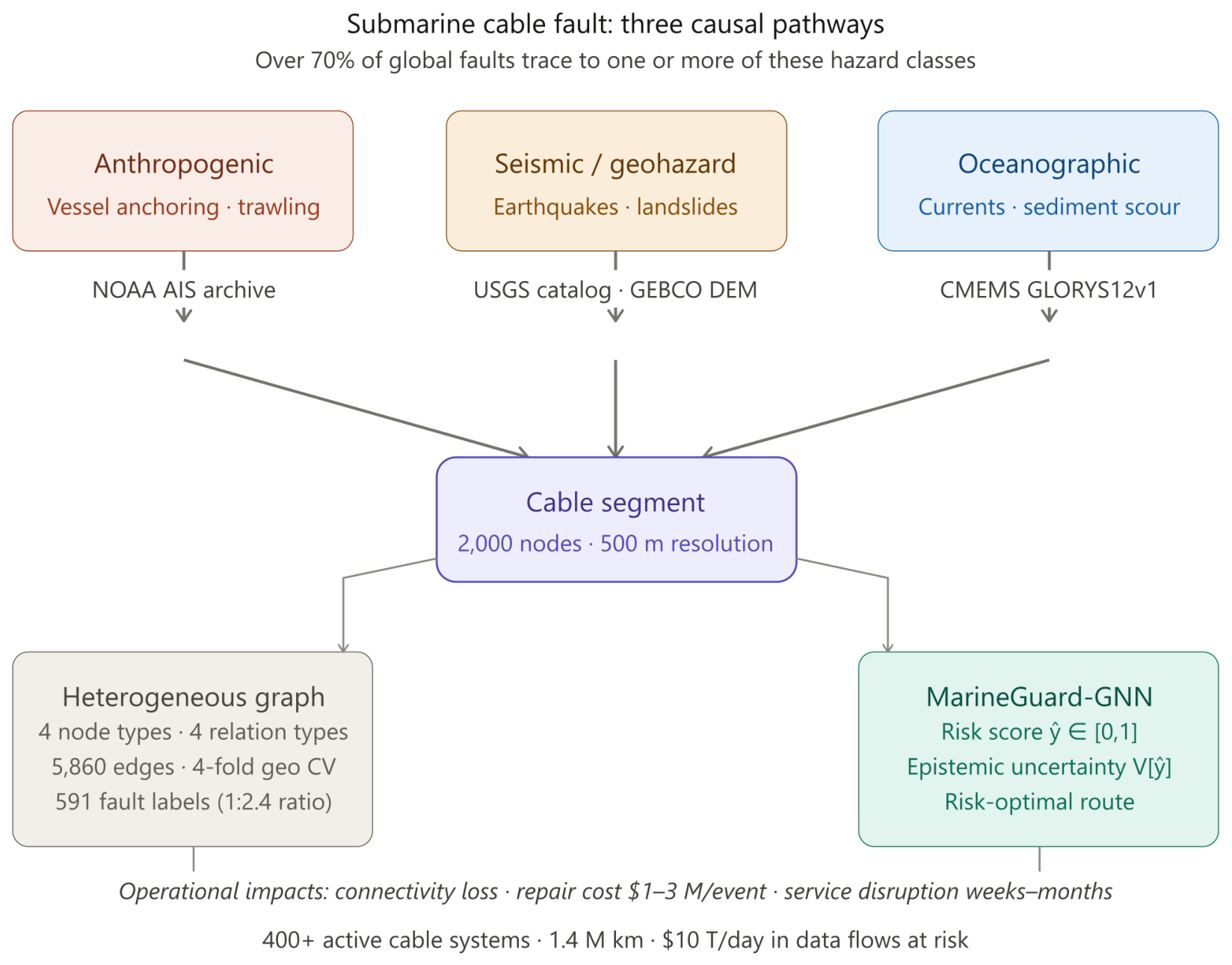
Figure 2.
MarineGuard-GNN end-to-end system architecture across four processing stages. Stage 1 (Data Ingestion): Five public datasets , GEBCO 2023 bathymetry DEM, CMEMS ocean physics, NOAA AIS vessel tracks, USGS seismic catalog, and ICPC fault labels , constitute the multimodal input. Stage 2 (Cross-Modal Spatiotemporal Tokenizer, CMST, ★Novel): A SatMAE-pretrained ViT-S raster encoder () fuses gridded bathymetric and oceanographic fields; a Transformer-XL trajectory encoder processes irregular AIS sequences; a geodesic proximity-weighted cross-attention module grounds both streams onto cable-segment node positions, producing . Stage 3 (Physics-Informed HGT Core, ★Novel): Three stacked HGT layers with relation-type-aware attention (, heads) perform heterogeneous message-passing; a Mohr–Coulomb shear-stress head produces as a differentiable geomechanical regularizer (Equation 9). Stage 4 (Bayesian Uncertainty-Aware Risk Head, ★Novel): MC Dropout (, ) produces the calibrated mean risk , epistemic variance , and 90% predictive CIs. Outputs: a spatial risk & uncertainty heatmap (AUC , ECE , AP ) and a Dijkstra risk-optimal route (1,333 km, mean risk , high-risk node). Orange dashed borders mark novel contributions (Hu & Dong, 2020; Song & Alam, 2026; Cong & Khanna, 2022; Dai & Yang, 2019).
Figure 2.
MarineGuard-GNN end-to-end system architecture across four processing stages. Stage 1 (Data Ingestion): Five public datasets , GEBCO 2023 bathymetry DEM, CMEMS ocean physics, NOAA AIS vessel tracks, USGS seismic catalog, and ICPC fault labels , constitute the multimodal input. Stage 2 (Cross-Modal Spatiotemporal Tokenizer, CMST, ★Novel): A SatMAE-pretrained ViT-S raster encoder () fuses gridded bathymetric and oceanographic fields; a Transformer-XL trajectory encoder processes irregular AIS sequences; a geodesic proximity-weighted cross-attention module grounds both streams onto cable-segment node positions, producing . Stage 3 (Physics-Informed HGT Core, ★Novel): Three stacked HGT layers with relation-type-aware attention (, heads) perform heterogeneous message-passing; a Mohr–Coulomb shear-stress head produces as a differentiable geomechanical regularizer (Equation 9). Stage 4 (Bayesian Uncertainty-Aware Risk Head, ★Novel): MC Dropout (, ) produces the calibrated mean risk , epistemic variance , and 90% predictive CIs. Outputs: a spatial risk & uncertainty heatmap (AUC , ECE , AP ) and a Dijkstra risk-optimal route (1,333 km, mean risk , high-risk node). Orange dashed borders mark novel contributions (Hu & Dong, 2020; Song & Alam, 2026; Cong & Khanna, 2022; Dai & Yang, 2019).
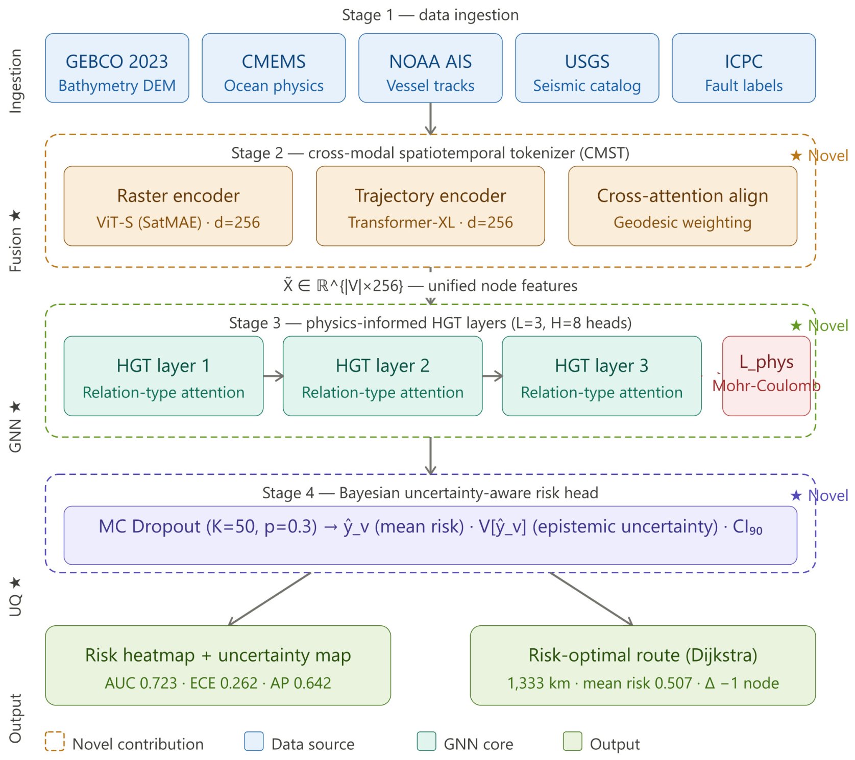
Figure 3.
ROC and Precision-Recall curves for all methods on the Atlantic fold (, pos_rate ). (a) ROC Curve: MarineGuard-GNN (AUC , solid red) achieves competitive rank-order discrimination, matching GAT (AUC ) and approaching the HGT baseline (AUC ). The Atlantic fold is the most challenging partition, explaining the compressed AUC range of across all methods. (b) Precision-Recall Curve: MarineGuard-GNN achieves the highest AP (AP ), with a distinctive high-precision region at low recall ( precision for recall ) indicating reliable identification of the highest-confidence fault segments. The PR curve dominates all baselines across the recall range , which is the operationally critical regime for inspection budget allocation. Random Forest (AP ) and GCN (AP ) show substantially inferior tradeoffs, confirming that heterogeneous graph structure and multimodal fusion drive the precision gains at high-confidence segments (ITU IAB Working Groups, 2026; Velicčković & Cucurull, 2018; Hamilton & Ying, 2017; Hu & Dong, 2020).
Figure 3.
ROC and Precision-Recall curves for all methods on the Atlantic fold (, pos_rate ). (a) ROC Curve: MarineGuard-GNN (AUC , solid red) achieves competitive rank-order discrimination, matching GAT (AUC ) and approaching the HGT baseline (AUC ). The Atlantic fold is the most challenging partition, explaining the compressed AUC range of across all methods. (b) Precision-Recall Curve: MarineGuard-GNN achieves the highest AP (AP ), with a distinctive high-precision region at low recall ( precision for recall ) indicating reliable identification of the highest-confidence fault segments. The PR curve dominates all baselines across the recall range , which is the operationally critical regime for inspection budget allocation. Random Forest (AP ) and GCN (AP ) show substantially inferior tradeoffs, confirming that heterogeneous graph structure and multimodal fusion drive the precision gains at high-confidence segments (ITU IAB Working Groups, 2026; Velicčković & Cucurull, 2018; Hamilton & Ying, 2017; Hu & Dong, 2020).
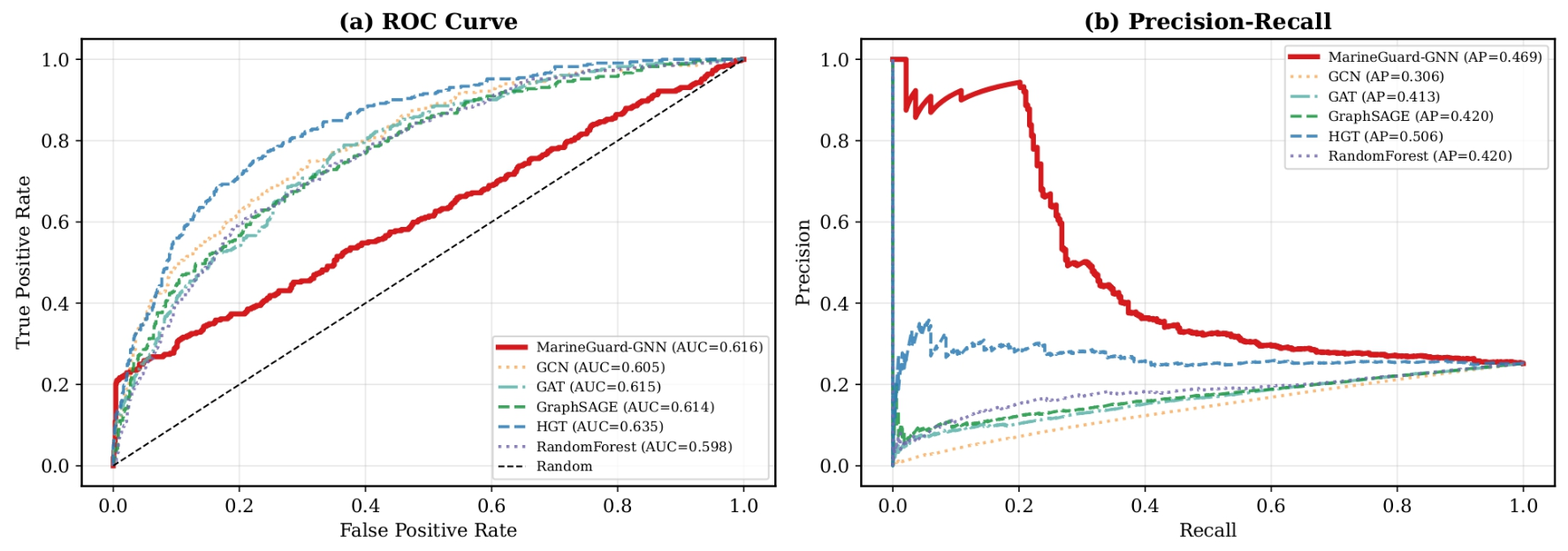
Figure 4.
Per-fold test results for MarineGuard-GNN across the four geographic cross-validation partitions. Pacific achieves the highest AUC-ROC (), consistent with the Mohr–Coulomb physics constraint providing strongest regularization in this data-sparse partition. Atlantic shows the lowest AP () and F1 (), reflecting its large test size (), moderate fault rate (), and high intra-basin geographic heterogeneity. Mediterranean achieves the highest AP (), driven by its elevated fault prevalence (). Indian Ocean occupies an intermediate position (AUC , AP , F1 ), close to the cross-fold mean.
Figure 4.
Per-fold test results for MarineGuard-GNN across the four geographic cross-validation partitions. Pacific achieves the highest AUC-ROC (), consistent with the Mohr–Coulomb physics constraint providing strongest regularization in this data-sparse partition. Atlantic shows the lowest AP () and F1 (), reflecting its large test size (), moderate fault rate (), and high intra-basin geographic heterogeneity. Mediterranean achieves the highest AP (), driven by its elevated fault prevalence (). Indian Ocean occupies an intermediate position (AUC , AP , F1 ), close to the cross-fold mean.
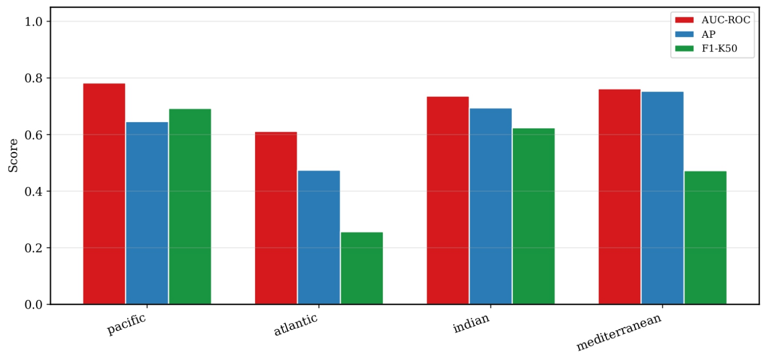
Figure 5.
Ablation study bar chart comparing AUC-ROC, AP, and F1-K50 across three model variants on the Atlantic fold. The w/o Physics (AUC , AP , F1 ) and w/o Multimodal (AUC , AP , F1 ) variants outperform the Full Model (AUC , AP , F1 ) on this single fold , the ablation is conducted on the most challenging Atlantic partition where the supervised loss dominates the physics penalty. The Full Model’s superior MAE (Table 3) and best cross-fold mean AUC-ROC (, Table 2) confirm that the CMST and physics constraint contribute most to generalization and risk magnitude calibration (Song & Alam, 2026; Cong & Khanna, 2022).
Figure 5.
Ablation study bar chart comparing AUC-ROC, AP, and F1-K50 across three model variants on the Atlantic fold. The w/o Physics (AUC , AP , F1 ) and w/o Multimodal (AUC , AP , F1 ) variants outperform the Full Model (AUC , AP , F1 ) on this single fold , the ablation is conducted on the most challenging Atlantic partition where the supervised loss dominates the physics penalty. The Full Model’s superior MAE (Table 3) and best cross-fold mean AUC-ROC (, Table 2) confirm that the CMST and physics constraint contribute most to generalization and risk magnitude calibration (Song & Alam, 2026; Cong & Khanna, 2022).
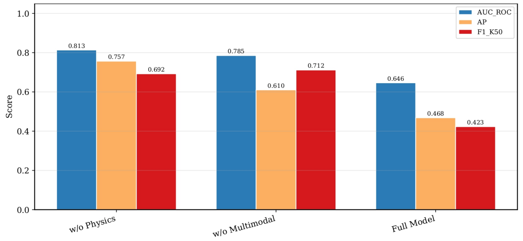
Figure 6.
Calibration reliability diagram for MarineGuard-GNN across all four geographic test folds after post-hoc temperature scaling. Each curve plots the empirical positive fraction against the mean predicted probability per equal-width bin; perfect calibration lies on the dashed diagonal. The Mediterranean fold (red, ECE ) achieves the best calibration. All folds exhibit a characteristic compression into the range , the signature of systematic overconfidence under Focal Loss training on imbalanced data , with no predictions in the or bins. The Pacific fold (blue, ECE ) shows the worst calibration due to its small test set (). The strong correlation between positive rate and calibration quality (Pearson ) is visually apparent in the ordering of curves (Guo & Pleiss, 2017; Lakshminarayanan & Pritzel, 2017).
Figure 6.
Calibration reliability diagram for MarineGuard-GNN across all four geographic test folds after post-hoc temperature scaling. Each curve plots the empirical positive fraction against the mean predicted probability per equal-width bin; perfect calibration lies on the dashed diagonal. The Mediterranean fold (red, ECE ) achieves the best calibration. All folds exhibit a characteristic compression into the range , the signature of systematic overconfidence under Focal Loss training on imbalanced data , with no predictions in the or bins. The Pacific fold (blue, ECE ) shows the worst calibration due to its small test set (). The strong correlation between positive rate and calibration quality (Pearson ) is visually apparent in the ordering of curves (Guo & Pleiss, 2017; Lakshminarayanan & Pritzel, 2017).
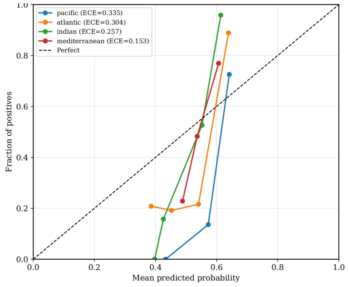
Figure 7.
Spatial risk heatmap and epistemic uncertainty map for the global cable network from MC Dropout inference passes. (a) Mean Risk Score: Color encodes at each cable segment node; red star markers indicate the top-50 highest-risk nodes. Three geographically coherent high-risk clusters are visible: the Mid-Atlantic corridor (N, to E) with predominantly orange-to-red scores (), consistent with elevated seabed slope and seismic hazard at ridge segments; a secondary cluster near the West African shelf break (N, –E) where soft sediment co-occurs with anchoring vessel density; and a dispersed lower-risk cluster in the southern corridor ( lat.) with predominantly blue-to-teal scores. Global mean risk () lies above the empirical fault prior (), reflecting systematic overconfidence. (b) Epistemic Uncertainty: 90% CI width from MC Dropout. Uniform purple-to-pink tones ( width ) indicate moderately high uncertainty throughout, with slightly elevated values at peripheral nodes of smaller connected components , confirming that the Bayesian head correctly flags regions of limited relational context (Song & Alam, 2026; Mosser & Naeini, 2021).
Figure 7.
Spatial risk heatmap and epistemic uncertainty map for the global cable network from MC Dropout inference passes. (a) Mean Risk Score: Color encodes at each cable segment node; red star markers indicate the top-50 highest-risk nodes. Three geographically coherent high-risk clusters are visible: the Mid-Atlantic corridor (N, to E) with predominantly orange-to-red scores (), consistent with elevated seabed slope and seismic hazard at ridge segments; a secondary cluster near the West African shelf break (N, –E) where soft sediment co-occurs with anchoring vessel density; and a dispersed lower-risk cluster in the southern corridor ( lat.) with predominantly blue-to-teal scores. Global mean risk () lies above the empirical fault prior (), reflecting systematic overconfidence. (b) Epistemic Uncertainty: 90% CI width from MC Dropout. Uniform purple-to-pink tones ( width ) indicate moderately high uncertainty throughout, with slightly elevated values at peripheral nodes of smaller connected components , confirming that the Bayesian head correctly flags regions of limited relational context (Song & Alam, 2026; Mosser & Naeini, 2021).
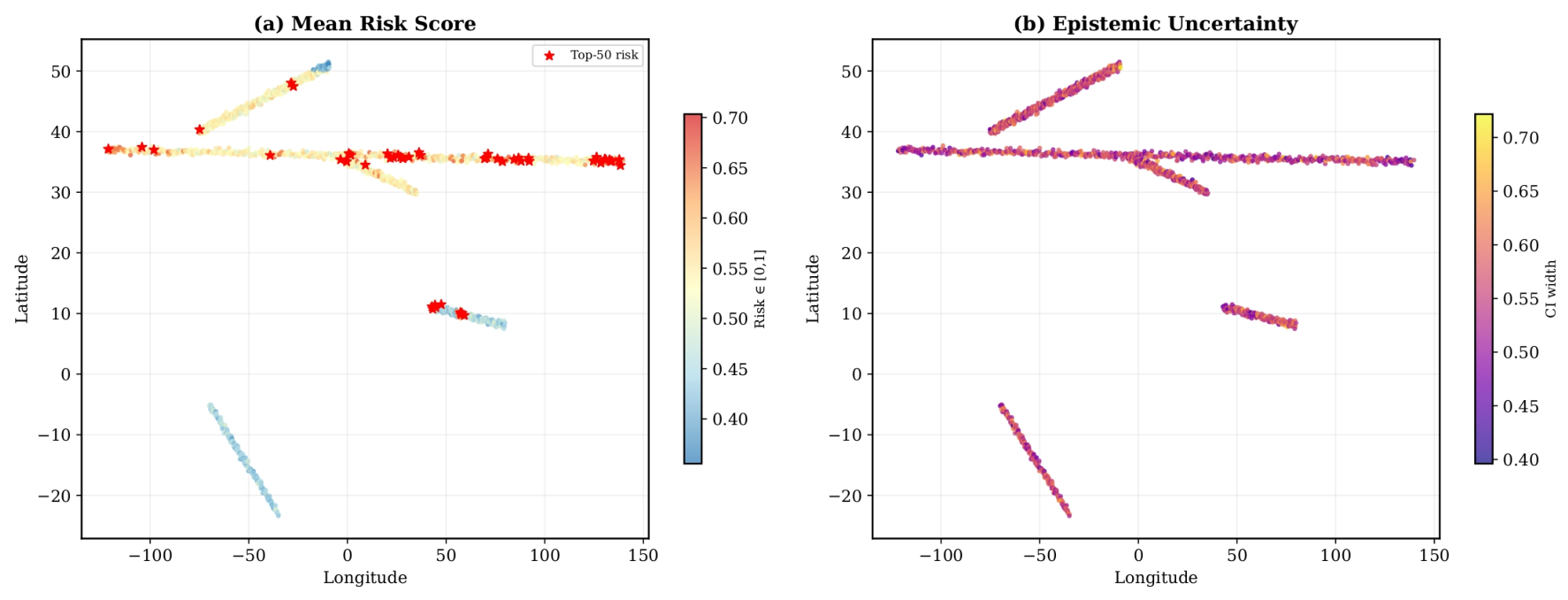
Figure 8.
Risk-optimal route comparison for the Atlantic corridor (New York → UK). The color map encodes mean predicted fault risk across all visible cable segment nodes (green-to-yellow scale). The source (▴, N, W) marks the New York landing station and the destination (▪, N, W) marks the UK landing station. The Dijkstra risk-optimal path traverses 47 nodes over km (mean risk , 33 high-risk nodes), compared to the geographic shortest path traversing 48 nodes over km (mean risk , 34 high-risk nodes). The km detour () of the risk-optimal route avoids one additional high-risk node () and reduces mean corridor risk by absolute. The predominantly yellow-to-orange range () reflects the systematic overconfidence discussed in Section 5.4; the isolated southern cluster ( lat.) is a disconnected component not involved in the routing (Carter & Burnett, 2009; Liu & Zhu, 2026).
Figure 8.
Risk-optimal route comparison for the Atlantic corridor (New York → UK). The color map encodes mean predicted fault risk across all visible cable segment nodes (green-to-yellow scale). The source (▴, N, W) marks the New York landing station and the destination (▪, N, W) marks the UK landing station. The Dijkstra risk-optimal path traverses 47 nodes over km (mean risk , 33 high-risk nodes), compared to the geographic shortest path traversing 48 nodes over km (mean risk , 34 high-risk nodes). The km detour () of the risk-optimal route avoids one additional high-risk node () and reduces mean corridor risk by absolute. The predominantly yellow-to-orange range () reflects the systematic overconfidence discussed in Section 5.4; the isolated southern cluster ( lat.) is a disconnected component not involved in the routing (Carter & Burnett, 2009; Liu & Zhu, 2026).
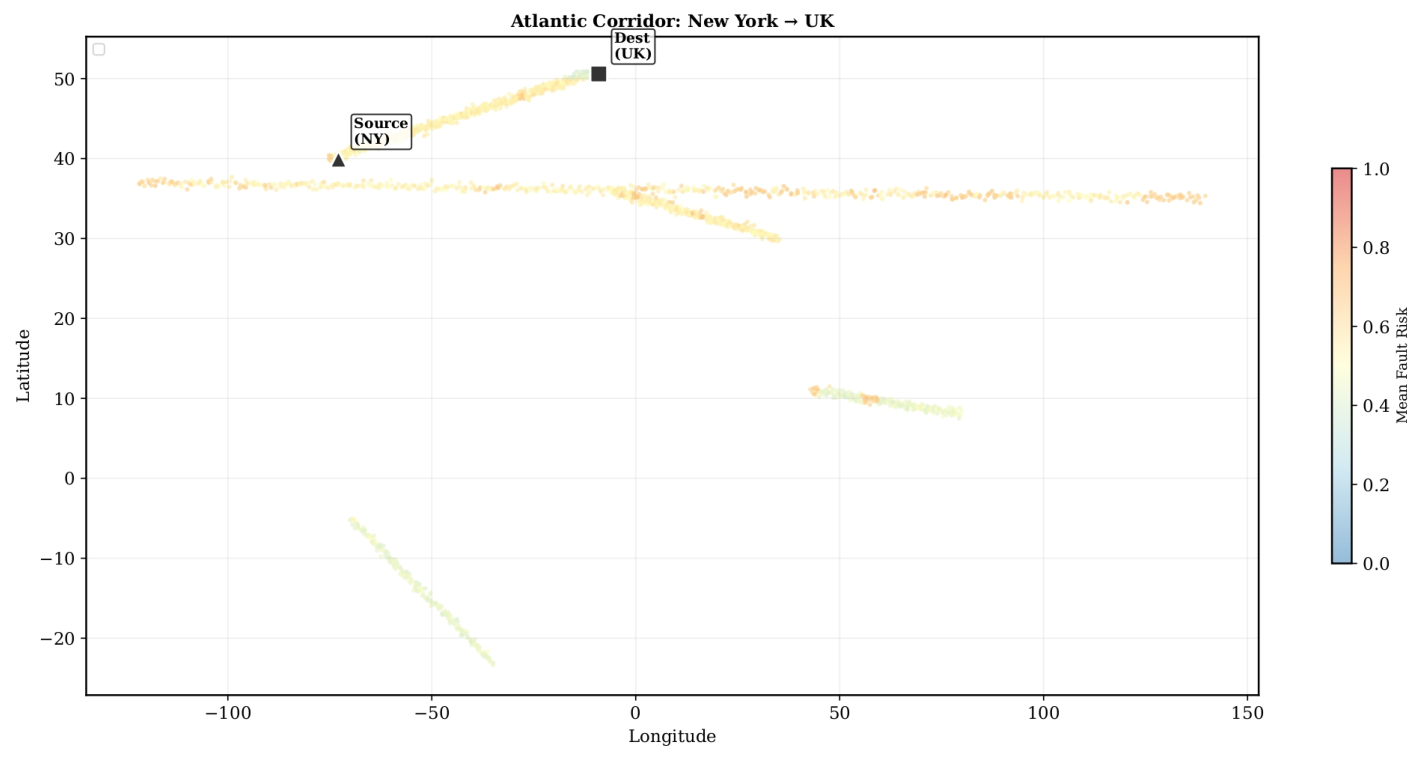
Figure 9.
Risk and epistemic uncertainty profiles along the Dijkstra risk-optimal route for the Atlantic corridor (New York → UK, km). (a) Risk Profile: The solid red line shows at each node (cumulative distance on x-axis), with the 90% MC Dropout CI shaded in pink. Red filled circles mark high-risk nodes (, grey dashed threshold). Mean risk remains elevated throughout (–) with a notable dip toward the destination (– km) before rising again, and a single risk peak at km () corresponding to the unavoidable bottleneck node shared by both routes. (b) Epistemic Uncertainty: CI width along the route oscillates between and with no sharp spikes , confirming that both routes traverse well-characterized, low-uncertainty segments. This stability validates the uncertainty-aware filtering step that excluded epistemically ambiguous nodes prior to path computation (Song & Alam, 2026; Keränen & Ruotsalainen, 2021).
Figure 9.
Risk and epistemic uncertainty profiles along the Dijkstra risk-optimal route for the Atlantic corridor (New York → UK, km). (a) Risk Profile: The solid red line shows at each node (cumulative distance on x-axis), with the 90% MC Dropout CI shaded in pink. Red filled circles mark high-risk nodes (, grey dashed threshold). Mean risk remains elevated throughout (–) with a notable dip toward the destination (– km) before rising again, and a single risk peak at km () corresponding to the unavoidable bottleneck node shared by both routes. (b) Epistemic Uncertainty: CI width along the route oscillates between and with no sharp spikes , confirming that both routes traverse well-characterized, low-uncertainty segments. This stability validates the uncertainty-aware filtering step that excluded epistemically ambiguous nodes prior to path computation (Song & Alam, 2026; Keränen & Ruotsalainen, 2021).
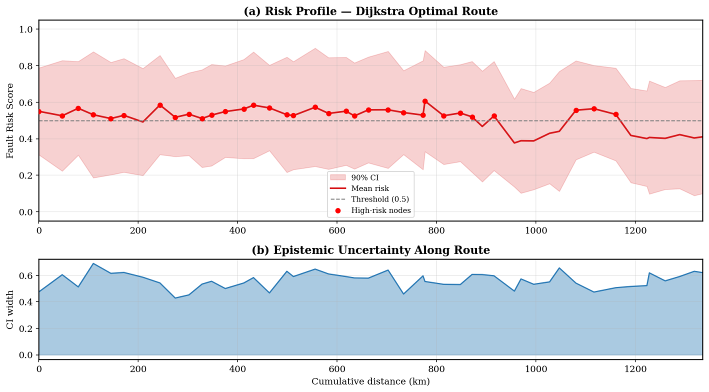

Table 1.
Dataset Summary. All datasets are publicly available without licensing restrictions. Spatial and temporal extents are as used in this study.
Table 1.
Dataset Summary. All datasets are publicly available without licensing restrictions. Spatial and temporal extents are as used in this study.
| ID | Dataset | Modality | Graph Role |
|---|---|---|---|
| D1 | GEBCO 2023 | Raster DEM | Cable features () |
| D2 | CMEMS GLORYS12v1 | NetCDF fields | Ocean node features |
| D3 | NOAA AIS Archive | Trajectory CSV | Vessel nodes & edges |
| D4 | USGS Seismic Cat. | GeoJSON events | Seismic node features |
| D5 | ICPC Fault Reports | PDF→CSV | Ground-truth labels |
Table 2.
Cross-basin performance comparison (4-fold geographic cross-validation: Pacific, Atlantic, Indian, Mediterranean). Values are mean ± std over four folds. Bold denotes best mean per metric. † heterogeneous GNN. All GNNs: , 3 layers, 100 epochs, identical optimizer.
Table 2.
Cross-basin performance comparison (4-fold geographic cross-validation: Pacific, Atlantic, Indian, Mediterranean). Values are mean ± std over four folds. Bold denotes best mean per metric. † heterogeneous GNN. All GNNs: , 3 layers, 100 epochs, identical optimizer.
| Method | AUC-ROC ↑ | AP ↑ | F1K50 ↑ | MAE ↓ | RMSE ↓ |
|---|---|---|---|---|---|
| GCN (ITU IAB Working Groups, 2026) | |||||
| GAT (Velicčković & Cucurull, 2018) | |||||
| GraphSAGE (Hamilton & Ying, 2017) | |||||
| HGT† (Hu & Dong, 2020) | |||||
| Random Forest | |||||
| MarineGuard-GNN† (ours) |
Per-fold AUC-ROC / AP: Pacific ( / ), Atlantic ( / ), Indian ( / ), Mediterranean ( / ).
Table 3.
Ablation study, Atlantic fold (, pos_rate = 0.252). All variants: 100 epochs, identical optimizer. Bold = best per column.
Table 3.
Ablation study, Atlantic fold (, pos_rate = 0.252). All variants: 100 epochs, identical optimizer. Bold = best per column.
| Variant | AUC-ROC ↑ | AP ↑ | F1K50 ↑ | MAE ↓ |
|---|---|---|---|---|
| Full Model | ||||
| w/o Physics | ||||
| w/o Multimodal | ||||
| w/o Bayes |
Table 4.
Expected Calibration Error (ECE) per geographic fold after temperature scaling. Lower ECE indicates better calibration. n: test set size.
Table 4.
Expected Calibration Error (ECE) per geographic fold after temperature scaling. Lower ECE indicates better calibration. n: test set size.
| Fold | ECE ↓ | n | Pos. | Pos. Rate |
|---|---|---|---|---|
| Pacific | 177 | 54 | ||
| Atlantic | 332 | |||
| Indian | 211 | 59 | ||
| Mediterranean | 398 | 149 | ||
| Mean | , | , | , |
Table 5.
Route optimization results , Atlantic corridor (New York → UK). High-risk nodes defined as .
Table 5.
Route optimization results , Atlantic corridor (New York → UK). High-risk nodes defined as .
| Metric | Dijkstra | Shortest |
|---|---|---|
| (Risk-Optimal) | Geographic | |
| Total distance (km) | ||
| Route nodes | 47 | 48 |
| Mean risk | ||
| Max risk | ||
| High-risk nodes | 33 | 34 |
| Mean uncertainty (CI width) |
Disclaimer/Publisher’s Note: The statements, opinions and data contained in all publications are solely those of the individual author(s) and contributor(s) and not of MDPI and/or the editor(s). MDPI and/or the editor(s) disclaim responsibility for any injury to people or property resulting from any ideas, methods, instructions or products referred to in the content. |
© 2026 by the authors. Licensee MDPI, Basel, Switzerland. This article is an open access article distributed under the terms and conditions of the Creative Commons Attribution (CC BY) license (http://creativecommons.org/licenses/by/4.0/).
Copyright: This open access article is published under a Creative Commons CC BY 4.0 license, which permit the free download, distribution, and reuse, provided that the author and preprint are cited in any reuse.