

Submitted:
21 July 2026
Posted:
22 July 2026
You are already at the latest version
Abstract
The transition to a low/non-carbon energy system requires both (i) further electrifying energy services and (ii) increasing the generation of that electricity from nonfossil fuels. We contribute to the nascent but growing literature on how energy prices impact the electrification of energy services by considering OECD country macro panel data and the electrification rates (share of energy consumption from electricity) of the residential and industrial sectors. For both sectors, we find a negative, significant, but relatively small (around -0.1 to -0.07) response for electricity prices and a positive, significant, and small (around 0.1 to 0.05) response for an index of direct use fossil fuel (e.g., coal, peat, natural gas, and oil products) prices. So, the combination of carbon taxes and encouraging renewables in electricity generation could harness both price incentives to in-crease electrification.
Keywords:
electrification
; electricity prices
; cross-price elasticity
; direct use of fossil fuels prices
; long macro-panel analysis
1. Introduction
Sustaining declining carbon emissions, i.e., decarbonizing the energy system, requires increasing both the share of energy services that are delivered via electricity and the share of nonfossil fuels used to generate that electricity [1]. Yet, there is evidence that high electricity prices (combined with fossil fuel prices that ignore carbon-based costs) discouraged households (in California) from switching to electricity for energy services like space heating, water heating, and personal mobility [2].
The current paper considers how electricity prices and the price of the direct use of fossil fuels contribute to electrification (share of energy consumption from electricity) in the residential and industrial sectors. It does so by analyzing OECD country macro panel data spanning 1978-2017 using a mean group-based estimator. For both sectors, we find a negative, significant, but relatively small (ranging from -0.1 to -0.07) response for electricity prices and a positive, significant, and small (ranging from 0.1 to 0.05) response for the direct use of fossil fuel price index.
While there is a growing literature on determining how energy prices impact the adoption of electricity services, most of this work has focused on electric vehicles (e.g., [3,4,5]). Indeed, the only paper we know of like the current paper is [6]. Huntington [6] estimated the extent to which electricity prices deterred economy-wide electrification (i.e., the share of total energy use accounted for by electricity) by analyzing OECD country macro data spanning 1980-2019. That paper calculated an electricity price coefficient that ranged from -0.3 to -0.1.
The present paper goes beyond [6] in two important ways: (i) we focus on electrification in the residential and industry sectors; and (ii) we develop a real price index of the direct use of fossil fuels in those sectors, i.e., we estimate a cross-price elasticity of electrification. Huntington [6] considered economy-wide energy prices in addition to economy-wide electricity prices; but the extent to which economy-wide energy prices are comprised of economy-wide electricity prices is determined by the electrification rate (i.e., as electrification approaches 100%, the two prices converge).
2. Materials and Methods
2.1. Dataset
We define electrification as the final electricity consumption in a sector (residential or industry) divided by the total energy consumption in that sector. These data are from the IEA’s World Energy Balances. Real GDP per capita data are from the World Bank Development Indicators. Real electricity prices are from Enerdata’s Global Energy & CO2 database. The real price index of direct use of fossil fuels (coal, peat, and oil shale; natural gas; and oil products) for each sector (residential, industry) are constructed—as standard—by weighing Enerdata’s real price data for a specific fossil fuel by that fuel’s consumption share from the IEA’s Energy Balances. Table 1 lists each variable with details on its definition and source.
The final dataset consists of two balanced panels that span 1978-2017. The availability of the price data for the direct use of fossil fuels is why the panel ends in 2017 (the other series extend to 2019). The industry panel has 25 countries, and the residential panel has 24 (because Portugal does not have the residential fossil fuel price index, it is dropped from that panel). Table 2 presents descriptive statistics. The cross-sectional dependence test (CD test) from [7] indicates a strong degree of cross-sectional correlation for all variables, and most variables have high mean correlation coefficients.
Table 3 and Table 4 display electrification data at different points in time for the residential and industry sectors, respectively, for each country in the analysis. Even among OECD countries, residential electrification can have dramatic differences. For example, current rates are particularly high for Norway and New Zealand (85 and 72%, respectively) but is only 12% for Poland. Nearly all countries have experienced growth in electrification (Poland, too, but not Germany). Yet, for several countries there has been little change either recently (since 2010), like Australia, or for some time (since 1990), like Belgium, Denmark, and New Zealand. Other countries have grown in fits like Norway, Spain, and Switzerland.
Industry electrification shows less divergence (Table 4). Norway is still particularly high at 64%, but most countries are in the 30-40% range most recently. Finland has experienced little change throughout the time period, while Austria, Japan, Norway, Sweden, and Switzerland have had little change since 1990. In the US, industry electrification peaked in 2000 and has declined since then.
Figure 1 a&b present a last look at the dataset. These figures display the individual country traces for the industry real electricity price (Figure 1a) and the industry direct use of fossil fuel real price index (Figure 1b). For most (but not all) countries the residential and industry electricity price series are highly correlated as are the residential and industry fossil fuel price indices. Thus, to economize space, only the industry price series are shown. The fossil fuel price index (Figure 1b) clearly indicates the two major international oil price spikes: first in the early-to-mid 1980s and then again in the early 2010s. For electricity prices (Figure 1a), the traces are more diverse but most/many countries experienced declining prices.
2.2. Model and Method
Following [6], we model electrification (Elec) as a function of GDP per capita (GDP) and electricity prices (elec pr):
where t represents the time dimension, i the country dimension, and εit is the error term. Additionally, we include a price index of direct fossil fuel use (ff pr). We expect electricity price to have a negative coefficient and direct fossil fuel use price—as a cross-price term—to have a positive coefficient. However, we do not expect prices to have a contemporaneous impact on electrification; so, we lag those terms. Yet, we do not have a priori knowledge on what the lag structure should be; so, for robustness we consider up to three lags (a fourth lag or greater always produced insignificant coefficients). Again, because of a lack of a priori intuition and for robustness, we consider pairs of lagged price terms sequentially (i.e., leading to three regressions).
We also allow for an individual country time trend (trend). Time trends have been suggested to approximate technology/energy efficiency improvements in energy demand models (e.g., [8,9]). Huntington [6] does not motivate the inclusion of GDP per capita other than to acknowledge that electrification is considered part of the development/economic growth process. One might hypothesize that GDP represents the resources to afford infrastructure investments that make the electrification of energy services more attractive. Such investments would be done on the individual country level. Whereas, time trends represent technological improvements that encourage/facilitate electrification that all OECD countries are likely to find accessible (e.g., via trade/transfer) even when an individual country’s GDP growth stalls.
We analyze the residential and industry sectors in separate equations, but to avoid clutter do not include any more sub-/super-scripts in Equation 1. Lastly, we take natural logs of all the variables so that their coefficients can be interpreted as elasticities.
Although we are interested in panel coefficients, we use the mean group estimator from [10] that makes the most general assumption that the individual country coefficients are different and then averages those estimations to arrive at the panel coefficients (standard errors are constructed nonparametrically). Indeed, the Pasaran and Yamagata [11] test for slope homogeneity (results not shown) confirms that mean group panel average coefficients are different from fixed effects coefficients, i.e., fixed effects would be biased.
As the CD test results reported in Table 2 suggested, residual cross-sectional dependence (CSD) could be an issue. Untreated CSD in regression residuals suggests omitted variable bias and endogeneity, and thus, biased and inconsistent estimates. This problem is typically addressed in mean group regressions by adding cross-sectional average terms. Since, international energy prices are likely to be the main source of such dependence in our model (e.g., see Figure 1b), we include one (international energy prices) cross-sectional average. Data from the IEA Real Price Index for industry and households was used to construct the term. As will be discussed/shown in the following section, adding this one cross-sectional average variable removed evidence of stronger CSD; so, to preserve degrees of freedom, we add only one cross-sectional average term.
3. Results and Discussion
Table 5 displays the regression results; the bottom rows contain diagnostic statistics. There is a concern that the CD test from [7] over-rejects weak dependence when applied to residuals; so, as a residual diagnostic, we use the bias corrected CD* test from [12]. Since weak cross-sectional dependence could not be rejected (second to last row), we employ the Maddala and Wu [13] panel unit root test to demonstrate that the residuals are stationary (last row). (The CIPS test [14] was used to demonstrate stationarity for the one case that marginally rejected weak dependence, i.e., residential electrification with three-year lags).
The electricity price coefficients are negative, always statistically significant, but relatively small—always around -0.1 for residential and always less than -0.1 (ranging from -0.08 to -0.07) for industry. The fossil fuel price coefficients are positive, usually significant, and mostly of similar (absolute) magnitude as the electricity price coefficients. These fossil fuel price coefficients ranged from 0.1 to 0.05 for residential and, when significant, from 0.09 to 0.06 for industry (depending on the lag). The time trend is positive, always significant, but even smaller in absolute magnitude. The GDP coefficient is always significant and large for industry, but it is significant for only one regression for residential. Huntington’s [6] most similar regression produced a larger electricity price coefficient of -0.3 and a smaller GDP coefficient of 0.2 (both highly statistically significant).
Huntington [6] raised the issue of endogeneity between electrification and economic growth. This endogeneity is unlikely for the residential sector but could exist for the industry sector since electricity is considered a more/the most productive form of energy. However, the GDP term in our model is aggregate output per capita and not industry output. Furthermore, for the developed OECD countries in our panel, industry’s share of GDP is rather small; e.g., it is mostly below 30%. Further still, industry’s share of GDP is negatively correlated with GDP per capita for nearly every country (Ireland and Norway are the exceptions). Huntington [6] tried to instrument for GDP using the output shares of agriculture, construction, industry, and services. Not only does this instrument seem inappropriate for our purposes (e.g., the dependent variable is electrification for industry only), it would lead to several years of lost data. Ultimately, [6] argued that for richer (i.e., OECD) countries, economic growth should cause electrification (in other words, endogeneity was not a concern). Nevertheless, for robustness, we consider two alternative specifications for the industry panel: (i) drop GDP (as did [6]); and (ii) replace contemporaneous GDP with its one-year lag to further mitigate any possible endogeneity. Those results—shown in Appendix Table A1—are mostly in concert with the results from Table 5.
5. Conclusions
Liddle and Parker [1] determined that, for the 15 countries that have sustained reductions in their per capita CO2 emissions and decoupled those emissions from GDP (i.e., their emissions and GDP are negatively associated/correlated), they decarbonized their energy systems by increasing both the share of energy services that are delivered via electricity and the share of nonfossil fuels used to generate that electricity. Yet, there is a concern that high electricity prices deter the electrification process (e.g., [2,6]). This analysis determined that electricity prices do impede the electrification process in the residential and industrial sectors by a small amount. However, the analysis also found that direct use of fossil fuel prices encourage electrification by a mostly similar small amount. Hence, there is a policy opportunity to harness these dual (albeit modest) price incentives to simultaneously encourage electrification by coupling carbon taxes with renewable inducements/subsidies (i.e., raising the price of the direct use of fossil fuels relative to the price of electricity).
Funding
This research received no external funding.
Data Availability Statement
Table 1 lists the availability/source of each variable used in the analysis. The empirical part of the paper used Stata. Specifically, the following routines were employed: xtdcce2 and xtcd2, which were developed by Jan Ditzen. xthst, which was developed by Tore Bersvendsen and Jan Ditzen. multipurt, which was developed by Markus Eberhardt.
Conflicts of Interest
The author declare no conflicts of interest.
Abbreviations
The following abbreviations are used in this manuscript:
| OECD | Organization for Economic Co-operation and Development |
| IEA | International Energy Agency |
| GDP | Gross domestic product |
Appendix A

Table A1.
Alternative specifications for industry electrification. Mean Group estimator from [10].
Table A1.
Alternative specifications for industry electrification. Mean Group estimator from [10].
| No GDP term | Lagged GDP | |||||
| GDP t-1 | 0.441*** (0.124) |
0.419*** (0.128) |
0.406*** (0.120) |
|||
| Trend | 0.014**** (0.0019) |
0.013**** (0.0018) |
0.012**** (0.0017) |
0.0064*** (0.0022) |
0.0060** (0.0024) |
0.0055** (0.0025) |
| Electricity price t-1 |
-0.759** (0.0330) |
-0.0604 (0.0371) |
||||
| Fossil fuel price index t-1 | 0.0725*** (0.0209) |
0.0837**** (0.0233) |
||||
| Electricity price t-2 |
-0.0846*** (0.0253) |
-0.0710** (0.0342) |
||||
| Fossil fuel price index t-2 | 0.0413** (0.0210) |
0.0575** (0.0236) |
||||
| Electricity price t-3 |
-0.0984*** (0.0328) |
-0.0773* (0.0405) |
||||
| Fossil fuel price index t-3 | 0.0200 (0.0278) |
0.0312 (0.0292) |
||||
| Obs | 975 | 950 | 925 | 975 | 950 | 925 |
| RMSE | 0.07 | 0.06 | 0.05 | 0.06 | 0.06 | 0.05 |
Notes: ****, ***, **, * indicate statistical significance at the 0.001, 0.01, 0.05, and 0.1 levels, respectively. Standard errors are in parentheses (constructed nonparametrically as described in [10]).
References
- Liddle, B.; Parker, S. Another look at ‘peak and decline’ carbon emissions countries: Which ones have decoupled per capita emissions from GDP and how? Glob. Environ. Change Adv. 2024, 3, 100012. [Google Scholar] [CrossRef]
- Borenstein, S.; Bushnell, J. Headwinds and Tailwinds: Implications of Inefficient Retail Energy Pricing for Energy Substitution. Environ. Energy Policy Econ. 2022, 3, 37–70. [Google Scholar] [CrossRef]
- Fei, Y.; Qin, P.; Chu, Y.; Zheng, H.; Tan-Soo, J.-S.; Zhang, X.-B. Does high gasoline price spur electric vehicle adoption? Evidence from Chinese cities. Energy Econ. 2025, 142, 108188. [Google Scholar] [CrossRef]
- Bushnell, J.; Muehlegger, E.; Rapson, D. Energy Prices and Electric Vehicle Adoption. J. Political Econ. Microecon. 2026. [Google Scholar] [CrossRef]
- Zhang, X.-B.; Xu, J.; Zheng, Y.; Sari, R.; Chu, Y. Electric vehicle adoption and energy prices: Empirical evidence from four Nordic countries. Energy Econ. 2026, 154, 109148. [Google Scholar] [CrossRef]
- Huntington, H. Do high power prices slow electrification? Some panel data evidence. Energy Policy 2025, 203, 114630. [Google Scholar] [CrossRef]
- Pesaran, M. Testing weak cross-sectional dependence in large panels. Econom. Rev. 2015, 34, 1089–1117. [Google Scholar]
- Webster, M.; Paltsev, S.; Reilly, J. Autonomous efficiency improvement or income elasticity of energy demand: does it matter? Energy Econ. 2008, 30, 2785–2798. [Google Scholar] [CrossRef]
- Hunt, L. C.; Ryan, D. L. Economic modelling of energy services: Rectifying misspecified energy demand functions. Energy Econ. 2015, 50, 273–85. [Google Scholar] [CrossRef]
- Pesaran, M.; Smith, R. Estimating long-run relationships from dynamic heterogeneous panel. J. Econom. 1995, 68, 79–113. [Google Scholar] [CrossRef]
- Pesaran, M. H.; Yamagata, T. Testing slope homogeneity in large panels. J. Econom. 2008, 142, 50–93. [Google Scholar] [CrossRef]
- Pesaran, M. H.; Xie, Y. A Bias-Corrected CD Test for Error Cross- Sectional Dependence in Panel Data Models with Latent Factors. Camb. Work. Pap. Econ. 2021, 2158. [Google Scholar]
- Maddala, G.S.; Wu, S. A comparative study of unit root tests with panel data and a new simple test. Oxf. Bull. Econ. Stat. 1999, 61(Special Issue), 631–652. [Google Scholar] [CrossRef]
- Pesaran, M. A simple panel unit root test in the presence of cross-section dependence. J. Appl. Econom. 2007, 22, 265–312. [Google Scholar] [CrossRef]
Figure 1.
a Industry electricity price (2015 US $/kWh), 1978-2017. See Table 1 for source. b Industry direct use of fossil fuel real price index, 1978-2017. See Table 1 for source.
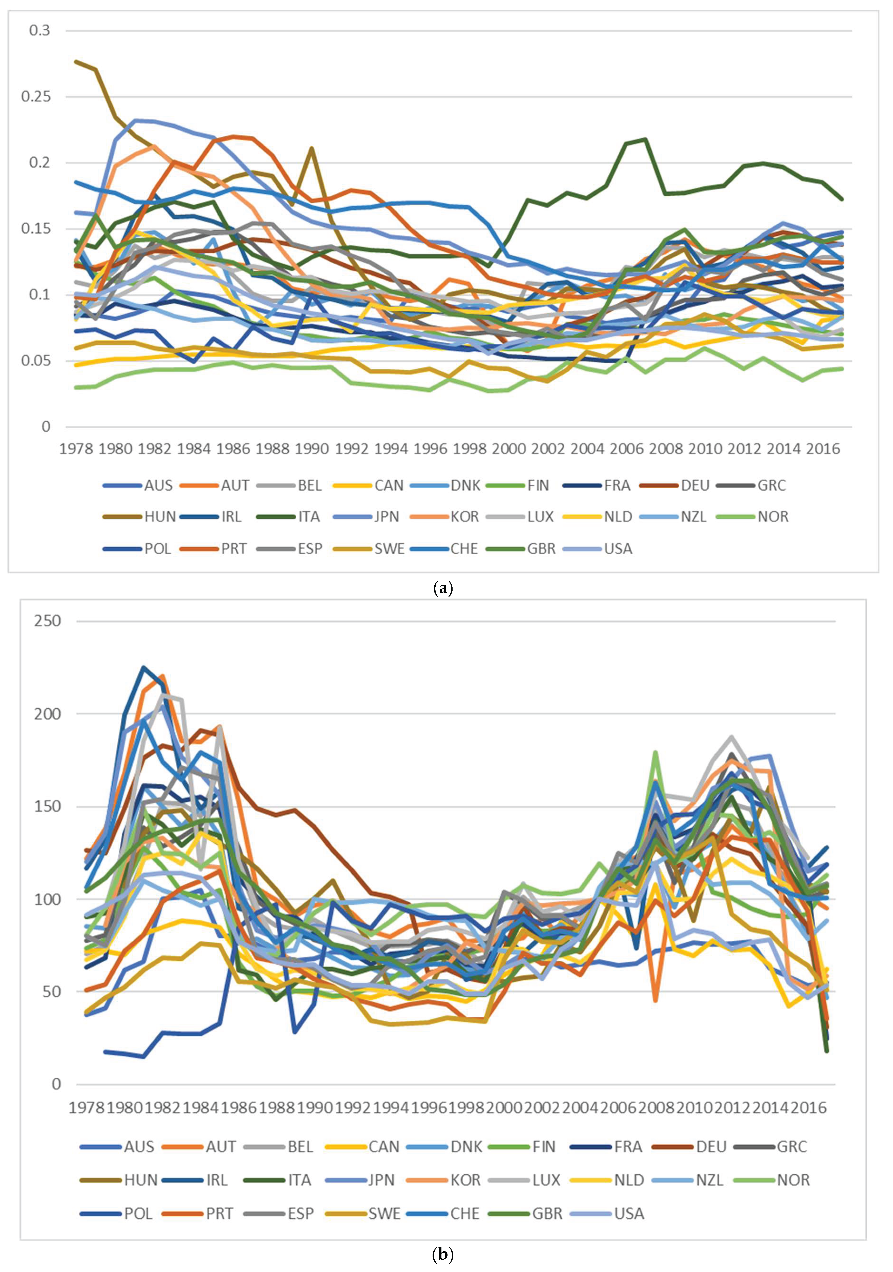
Table 1.
Variable definitions and sources used in analysis.
| Variable | Definition | Source |
| GDP | GDP per capita in constant 2015 US $ | World Bank Development Indicators https://databank.worldbank.org/source/world-development-indicators |
| R elec rt | Residential electrification rate in %: final electricity consumption in residential sector divided by total energy consumption in residential sector | IEA, World Energy Balances 2024. https://www.iea.org/data-and-statistics/data-product/world-energy-balances-highlights |
| I elec rt | Industry electrification rate in %: final electricity consumption in industry sector divided by total energy consumption in industry sector | IEA, World Energy Balances 2024. https://www.iea.org/data-and-statistics/data-product/world-energy-balances-highlights |
| R elec pr | Residential price of electricity (taxes included) in 2015 US $/kWh | Enerdata Global Energy & CO2 database. https://www.enerdata.net/research/energy-market-data-co2-emissions-database.html |
| I elec pr | Industry price of electricity (taxes included) in 2015 US $/kWh | Enerdata Global Energy & CO2 database. https://www.enerdata.net/research/energy-market-data-co2-emissions-database.html |
| R ff pr index | Residential real price index (2005) of direct use of fossil fuels (coal, peat, and oil shale; natural gas; and oil products) in residential sector | Author calculations from Enerdata price data and IEA World Energy Balance sector fuel share data. doi: 10.17632/7mp9d2dxbn.1 |
| I ff pr index | Industry real price index (2005) of direct use of fossil fuels (coal, peat, and oil shale; natural gas; and oil products) in industrial sector | Author calculations from Enerdata price data and IEA World Energy Balance sector fuel share data. doi: 10.17632/7mp9d2dxbn.1 |
Table 2.
Summary statistics and CD test from [7] with average correlation coefficients.
Table 2.
Summary statistics and CD test from [7] with average correlation coefficients.
| Variable | Mean | Std. Dev. | Min | Max | CD-test | Corr. coeff. |
| Residential panel 24 countries x 1978-2017 (960 balanced observations) | ||||||
| GDP | 35,576 | 18,879 | 3,914 | 112,418 | 98.6* | 0.939 |
| R elec rt | 29.1 | 17.6 | 4.1 | 83.7 | 75.7* | 0.721 |
| R elec pr | 0.18 | 0.06 | 0.02 | 0.34 | 13.6* | 0.129 |
| R ff pr index | 101.1 | 40.0 | 1.5 | 254.0 | 59.0* | 0.561 |
| Industry panel 25 countries x 1978-2017 (1,000 balanced observations) | ||||||
| GDP | 34,798 | 18,899 | 3,914 | 112,418 | 102.4* | 0.935 |
| I elec rt | 30.2 | 9.5 | 10.4 | 71.2 | 72.1* | 0.658 |
| I elec pr | 0.10 | 0.04 | 0.03 | 0.28 | 38.1* | 0.38 |
| I ff pr index | 96.6 | 36.3 | 14.8 | 225.1 | 68.8* | 0.628 |
Notes: * p-value < 0.001. Null hypothesis is weak cross-sectional dependence. Corr. coeff.=mean correlation coefficient. Variables in natural logs for CD-test; otherwise variable units as described in Table 1.
Table 3.
Individual country residential electrification rates over time.
| 1980 | 1990 | 2000 | 2010 | 2020 | |
| Australia | 41.2 | 44.2 | 46.3 | 50.9 | 49.6 |
| Austria | 14.8 | 17.4 | 20.3 | 21.8 | 25.0 |
| Belgium | 11.8 | 19.1 | 21.5 | 17.9 | 20.7 |
| Canada | 25.8 | 35.5 | 38.0 | 43.0 | 46.4 |
| Denmark | 11.5 | 20.8 | 21.1 | 18.2 | 21.9 |
| Finland | 15.5 | 23.5 | 33.4 | 33.9 | 39.6 |
| France | 23.4 | 21.9 | 27.3 | 31.4 | 38.0 |
| Germany | 18.0 | 18.7 | 17.2 | 19.3 | 19.3 |
| Greece | 24.5 | 25.6 | 26.9 | 33.4 | 35.8 |
| Hungary | 8.4 | 11.8 | 15.1 | 14.5 | 17.7 |
| Ireland | 17.0 | 15.3 | 20.4 | 20.5 | 23.8 |
| Italy | 11.2 | 17.4 | 19.0 | 16.9 | 18.6 |
| Japan | 38.8 | 40.5 | 44.2 | 51.4 | 51.8 |
| Korea | 4.9 | 13.3 | 20.9 | 26.8 | 28.6 |
| Luxembourg | 7.5 | 9.9 | 14.5 | 13.7 | 16.5 |
| Netherlands | 9.2 | 13.0 | 15.9 | 15.9 | 21.1 |
| New Zealand | 68.2 | 72.1 | 70.4 | 73.5 | 72.3 |
| Norway | 60.8 | 72.3 | 77.9 | 76.5 | 84.8 |
| Poland | 4.6 | 9.8 | 10.5 | 11.2 | 12.4 |
| Spain | 32.8 | 28.3 | 31.3 | 38.5 | 43.9 |
| Sweden | 22.7 | 50.1 | 49.5 | 47.8 | 51.0 |
| Switzerland | 16.1 | 22.1 | 24.9 | 26.2 | 33.6 |
| United Kingdom | 20.6 | 21.6 | 22.3 | 22.8 | 26.1 |
| United States | 28.6 | 37.9 | 38.8 | 46.0 | 48.2 |
Table 4.
Individual country industry electrification shares at different points in time.
| 1980 | 1990 | 2000 | 2010 | 2020 | |
| Australia | 15.9 | 26.3 | 27.8 | 32.0 | 30.1 |
| Austria | 24.7 | 29.5 | 29.5 | 29.7 | 31.2 |
| Belgium | 18.4 | 25.7 | 29.1 | 31.3 | 31.4 |
| Canada | 23.3 | 30.6 | 30.2 | 36.6 | 35.3 |
| Denmark | 15.8 | 27.0 | 29.4 | 30.3 | 32.6 |
| Finland | 32.8 | 30.7 | 31.8 | 32.0 | 30.0 |
| France | 19.9 | 31.3 | 35.1 | 35.3 | 36.7 |
| Germany | 21.8 | 28.1 | 35.4 | 34.6 | 33.2 |
| Greece | 23.3 | 26.1 | 26.2 | 35.0 | 40.4 |
| Hungary | 16.0 | 19.4 | 22.9 | 32.0 | 33.9 |
| Ireland | 12.7 | 21.8 | 27.2 | 29.0 | 26.0 |
| Italy | 22.6 | 28.0 | 31.9 | 36.5 | 42.1 |
| Japan | 30.9 | 34.2 | 35.2 | 35.9 | 36.7 |
| Korea | 18.9 | 24.5 | 34.2 | 40.7 | 47.5 |
| Luxembourg | 12.9 | 18.4 | 37.8 | 41.4 | 42.2 |
| Netherlands | 19.6 | 19.4 | 22.3 | 23.1 | 22.8 |
| New Zealand | 27.4 | 29.7 | 31.4 | 35.2 | 30.2 |
| Norway | 53.4 | 65.3 | 64.5 | 61.2 | 64.0 |
| Poland | 13.9 | 16.0 | 20.1 | 26.4 | 29.7 |
| Portugal | 21.2 | 22.6 | 22.3 | 27.5 | 31.1 |
| Spain | 24.7 | 28.3 | 29.9 | 30.2 | 31.5 |
| Sweden | 29.2 | 39.1 | 35.8 | 39.3 | 36.2 |
| Switzerland | 26.4 | 42.4 | 40.9 | 42.4 | 42.9 |
| United Kingdom | 19.1 | 26.9 | 28.9 | 34.4 | 34.5 |
| United States | 16.6 | 26.3 | 29.6 | 26.3 | 23.1 |
Table 5.
Regression results. Electrification rate dependent variable. Balanced data, 1978-2017. All variables in natural logs. Mean Group estimator from [10].
Table 5.
Regression results. Electrification rate dependent variable. Balanced data, 1978-2017. All variables in natural logs. Mean Group estimator from [10].
| Residential (24 countries) | Industry (25 countries) | |||||
| GDP | 0.169 (0.116) |
0.171 (0.108) |
0.270** (0.120) |
0.457*** (0.137) |
0.457*** (0.136) |
0.399*** (0.125) |
| Trend | 0.010**** (0.0020) |
0.0091**** (0.0016) |
0.0065**** (0.0017) |
0.0065*** (0.0023) |
0.0056** (0.0025) |
0.0068** (0.0026) |
| Electricity price t-1 |
-0.109* (0.0558) |
-0.0665* (0.0380) |
||||
| Fossil fuel price index t-1 | 0.111*** (0.0414) |
0.0913**** (0.0230) |
||||
| Electricity price t-2 |
-0.116** (0.0562) |
-0.0706** (0.0354) |
||||
| Fossil fuel price index t-2 | 0.0640** (0.0293) |
0.0603*** (0.0229) |
||||
| Electricity price t-3 |
-0.130** (0.0630) |
-0.0789** (0.0381) |
||||
| Fossil fuel price index t-3 | 0.0506** (0.0247) |
0.0301 (0.282) |
||||
| Observations | 936 | 912 | 888 | 975 | 950 | 925 |
| RMSE | 0.07 | 0.06 | 0.06 | 0.06 | 0.06 | 0.05 |
| CD* | 1.6 | 1.4 | 1.7* | -0.3 | -0.2 | 0.3 |
| MW/CIPS | I(0) | I(0) | I(0) | I(0) | I(0) | I(0) |
Notes: ****, ***, **, * indicate statistical significance at the 0.001, 0.01, 0.05, and 0.1 levels, respectively. Standard errors are in parentheses (constructed nonparametrically as described in [10]). Diagnostics: RMSE = root mean squared error. CD* = bias corrected CD test from [12] on residuals. The null hypothesis is weak cross-sectional dependence. MW= Maddala and Wu test [13] or CIPS= CIPS test [14] on residuals. The null hypothesis is nonstationary. I(0)=stationary.
Disclaimer/Publisher’s Note: The statements, opinions and data contained in all publications are solely those of the individual author(s) and contributor(s) and not of MDPI and/or the editor(s). MDPI and/or the editor(s) disclaim responsibility for any injury to people or property resulting from any ideas, methods, instructions or products referred to in the content. |
© 2026 by the authors. Licensee MDPI, Basel, Switzerland. This article is an open access article distributed under the terms and conditions of the Creative Commons Attribution (CC BY) license (http://creativecommons.org/licenses/by/4.0/).
Copyright: This open access article is published under a Creative Commons CC BY 4.0 license, which permit the free download, distribution, and reuse, provided that the author and preprint are cited in any reuse.


