
Submitted:
21 July 2026
Posted:
22 July 2026
You are already at the latest version
Abstract
This paper examined a machine-learning technique for classifying riverine land covers in satellite images at different times with their normalized indices. The satellite images captured a river course in Kurobe River, Japan, in November 2017 and November 2018. The machine learning technique examined in this study was RF (random forests). The riverine land covers were classified into the following classes: tree, grass, bare gravel/sand bed, and water surface. This study trained RF using satellite image features in November 2017. Then, it applied the trained RF to those in November 2018 to examine the RF applicability to new satellite images with different radiance. A permutation importance analysis tried to detect essential satellite image features between the following ones: four multispectral band components, i.e., red, green, blue, and near-infrared, as well as three normalized indices, i.e., NDVI (normalized difference vegetation index), NDWI (normalized difference water index), and BNDVI (blue NDVI). The results showed that the F-measure of RF with the three normalized indices had a higher value, 0.74, than that without them, 0.63. In addition, the permutation importance analysis of the RF classification indicated that BNDVI had the highest value among all image features. These results supported the usefulness of the normalized indices for the machine-learning-based classification of riparian land covers at different times with different radiance of satellite images.
Keywords:
river management
; land cover classification
; satellite image
; normalized indices
; random forests
; permutation importance analysis
1. Introduction
Many rivers worldwide have experienced vegetation expansion and overgrowth in the river courses for several decades [1,2,3,4,5,6,7,8,9,10,11,12]. This vegetation overgrowth tendency posed serious engineering problems in river management, such as reduced flood flow capacity due to the increased vegetation drag force and river ecosystem alterations due to the non-native vegetation invasion. Causes of vegetation overgrowth would vary in each river basin, depending on hydrological, hydraulic, geomorphological, and ecological characteristics [13,14,15,16]. Therefore, it would be of fundamental importance to continuously monitor riverine land cover changes in terms of both the flood control and ecological conservation points of view in river management. Conventionally, river monitoring has used aerial photographs by airplanes [17,18]. However, this method made it difficult to monitor the whole river system at a high frequency due to its cost and other preparations. Therefore, developing a new efficient method to monitor river courses with high frequency would be indispensable.
To monitor riverine land covers and implement river management appropriately, new remote sensing technologies have been introduced in river management, such as UAVs (unmanned aerial vehicles) and high-frequency satellites [19,20,21,22,23,24,25,26,27,28]. Since UAVs can easily acquire high-resolution images, many researchers have utilized them to classify riverine land covers. AI (artificial intelligence), such as machine learning, has also been applied to the RGB information of images to automatically detect vegetation and classify riverine land covers [19,20,21]. In recent years, satellite imagery has become readily available for riverine land covers and would be a promising method for a high-frequency classification of river systems. Moreover, using AI could improve the work efficiency and accuracy of the river land cover classification.
Previous studies that used satellite imagery to classify riverine land covers include a study that used MODIS (moderate resolution imaging spectroradiometer) imagery to analyze flooded zone changes in the middle reaches of the Yangtze River [22] and a study that created land cover maps for the wetlands in the Hudson River [23]. In addition, some studies examined riverine land covers by combining satellite imagery and machine learning [24,25,26]. However, these studies focused on land covers in whole river basins, including flood plains. There is no example of methodological development that tried to classify land covers within river channels. Moreover, these studies analyzed imagery at a specific time. They did not treat the temporal changes in riverine land covers by a single classification method, which would be helpful for river monitoring.
The authors proposed a machine learning method for classifying riverine land covers by RF (random forests) with the RGB and NIR (near-infrared) radiance information from satellite imagery and the corresponding high-resolution UAV images [27,28]. The proposed method could be applied to satellite images with different radiance information at other times. However, additional image features obtained from satellite images at the target time were required to optimize the machine learning model for a specific time [28]. It would require lots of effort because new image datasets for the new target time should be prepared in each riverine land cover to create image features for machine learning refinement.
To address this key research question, this study tried to use normalized indices, i.e., NDVI (normalized difference vegetation index), NDWI (normalized difference water index), and BNDVI (blue NDVI) for the image features of the machine learning, which would expect to overcome the radiance differences between satellite images by their normalization. This study examined the best possible combination of image features, including the normalized indices, NDVI, NDWI, and BNDVI, as well as the RGB and NIR radiance information, to obtain effective image features and classify accurate riverine land covers at different times.
2. Materials and Methods
2.1. Study Field
Figure 1 shows the elevation map of the target river basin, the Kurobe River basin. The main channel in the Kurobe River is 85 km long, and its basin area is 682 km2. The red line shown in Figure 1 is the river channel section examined in this study, where the UAV and satellite images were obtained for the machine learning application. This river channel section is located 4 – 6 km from the river mouth, where gravel riverbeds have developed with extensive vegetation overgrowth.
Table 1 summarizes the specification of the satellite and UAV images and Figure 2, Figure 3, Figure 4 and Figure 5 show the UAV and satellite images used in this study. The UAV images shown in Figure 2 and Figure 3 were taken in November 2017 and November 2018 by Momose et al. [20] with a multispectral camera of five bands (R/G/B/NIR/Red edge) in a 0.1m of spatial resolution. The target data creation areas indicated in Figure 2 and Figure 3 were used to detect true classes of riverine land covers. The satellite images in Figure 4 and Figure 5 with four bands (R/G/B/NIR) in a pixel size of 3m were used to examine a machine learning applicability. The satellite imagery used here was available to obtain daily basis at a frequency high enough for appropriate river management.
2.2. Riverine Land Cover Classification Procedure
Figure 6 shows this study's flowchart of the riverine land cover classification procedure. Based on the RGB images of the high-resolution UAV images in November 2017 and November 2018, shown in Figure 2 and Figure 3, the riverine land covers each year were detected manually to the following four true classes: water surface, bare gravel/sand bed, grass, and tree. These true classes of riverine land covers were used as the training data for machine learning and for validating classification accuracy. The true classes were coarse-grained to a pixel size of the satellite image, 3m x 3m. In addition, the datasets of image features for using machine learning were created based on the RGB and NIR data available from the satellite images. These datasets of true classes and image features in the red frames shown in Figure 2 and Figure 3 (7,991 pixels in total) were made from the portions where land covers did not change, and the land cover class was detected between the two years using the training data for machine learning. The tuned machine learning algorithm detected the land cover classes over the entire area within the red frames in Figure 4 and Figure 5 using the image feature datasets of satellite images. Finally, the classification accuracy of the four classes was verified using the permutation importance analysis.
2.3. Machine Learning Algorithm and Accuracy Evaluation Index
The machine learning algorithm used in this study was RF (Random Forests) [29]. RF is an ensemble machine learning method that combines several different decision trees [30,31]. RF can be trained efficiently by parallelization. It is characterized by fewer parameters with higher classification accuracy than other machine learning methods [29]. Moreover, it has been recently confirmed that it could classify riverine land covers with high accuracy [32].
The Python library, scikit-learn [33], was used to run the RF architecture. F-measure [34,35], the harmonic mean of Precision and Recall, was used to measure classification performance in machine learning. The formulae of the Precision, Recall, and F-measure were defined as follows:
where TP (True Positive): The number of pixels for which a land cover class in question was classified to be the true class determined by the machine learning, FP (False Positive): The number of pixels for which a land cover class out of question was classified to be the true class by the machine learning, FN (False Negative): The number of pixels for which a land cover class in question was classified to be a false class by the machine learning.
2.4. Datasets of Image Features for Developing the Machine Learning Model
Table 2 summarizes the datasets of image features to examine their usefulness for machine learning. The six cases were set up using a combination of possible image features available from the satellite images used in this study.
The dataset Case 1 consists of the raw RGB (Red, Green, and Blue) and NIR radiance bands obtained from satellite imagery in November 2017. Case 2 used the same data as Case 1 but standardized to the values between -1 and 1 based on the radiance distribution of the target areas. Case 3 consists of the normalized indices of NDVI [36], NDWI [37], and BNDVI [38], which were calculated from the following formulas:
NDVI, NDWI, and BNDVI were the normalization indices between -1 and 1 calculated using the RGB and NIR radiance values. Assuming that the effect of differences in radiance in satellite images at different times would be almost the same for all wavelengths from the RGB bands to the NIR band, the NDVI, NDWI, and BNDVI could reduce the effect of the radiance differences in their distributions.
Cases 4 and 5 consisted of the combinations of image features used in Cases 1, 2, and 3. Case 6 used the raw radiance values in RGB and NIR bands from the satellite images in November 2017 and November 2018 to obtain the riverine land cover classification with possible high accuracy. Therefore, Case 6 should be treated as a reference case to determine useful image features in the machine learning algorithm. Adding the image features of the November 2018 satellite imagery could improve the accuracy of land cover detection classification.
2.5. Importance Evaluation of Features
RF is a machine learning method that improves general decision-making ability by combining multiple decision trees. However, its structure becomes complex, and it is difficult to grasp the relationship between image features and detection accuracy.
This study used PIMP (permutation importance) to analyze the image features important for detecting riverine land cover classes. PIMP is a method for determining the image features that have a relatively large impact on the accuracy of riverine land cover classification. It compared the prediction accuracy of randomly rearranged image features in the tuned RF model with the original prediction accuracy [39,40]. Specifically, PIMP sorted only one type of image feature in the RF model, and the relative importance of the image feature was evaluated based on the amount of reduction in accuracy when sorted. The higher the importance of the image feature was, the more it contributed to the classification accuracy.
3. Results
3.1. Image Features of Riverine Land Covers
Figure 7 shows the histograms of radiance distributions in the four bands, R/G/B/NIR, in each lane cover class obtained from the satellite images in November 2017 and November 2018. Figure 8 shows similar histograms for the four normalized indices, NDVI/NDWI/BNDVI, in the land cover classes in November 2017 and November 2018.
Comparison of Figure 7 (a) with Figure 7 (b) indicates that there is no significant difference in the distribution characteristics of each image feature and the relationship between the different image features. In addition, the radiance distributions of grass and tree in Figure 7 indicated that the R/G/B bands have almost the same distributions between the grass and tree.
Comparison of the normalized indices NDVI/NDWI/BNDVI in Figure 8(a) and (b) for each land cover class confirms that the distribution characteristics of NDVI, NDWI, and BNDVI are almost identical between the two timings, November 2017 and November 2018. This result suggests that these normalized indices has reduced the influence of the strong radiance differences in the different satellite images.
3.2. RF Machine Learning Classification of Riverine Land Covers
Figure 9 shows the distributions of riverine land cover classification by the RF machine learning method with the datasets of different image features for the satellite image in November 2018. Table 3 summarizes F-measure values in Cases 1-6 for riverine land cover classification accuracy in November 2018.
In Case 1, in which the trained RF with raw RGB and NIR information in November 2017 was applied to the November 2018 satellite image, the F-measure listed in Table 3 has 0.63 for all land cover classes. It confirmed that no grass was detected in Figure 9(b). Figure 4 and Figure 5 show that the satellite images in the two timings had much different radiance characteristics, particularly of the glass and tree classes, due mainly to the atmospheric conditions. These differences in radiance characteristics between the two satellite images could have an influence on the RF learning efficiency for detecting the riverine land covers.
The result in Case 2, shown in Figure 9(c), shows that the grass and tree classes were detected with the F-measure of 0.59 and 0.54, respectively. The accuracy in Case 2 was improved compared to that in Case 1 when using the standardized RGB and NIR instead of the raw ones. However, the F-measure for all land cover classes listed in Table 3 was 0.49 since many bare gravel/ sand bed locations were misclassified as water surfaces, resulting in an F-measure of 0.48 for the bare gravel/ sand bed class.
In Case 3, using the normalized indices NDVI, NDWI, and BNDVI, the F-measure listed in Table 3 reached a high accuracy of 0.74 for all land cover classes. It suggests the usefulness of the normalized indices NDVI, NDWI, and BNDVI for detecting the grass class by the RF architecture. On the other hand, a comparison of Figure 9(d) with Figure 9(a) indicates that the RF in Case 3 was a tendency for the grass class to be misclassified to the tree class, resulting in an F-measure of 0.44 for the grass class.
The results in Cases 4 and 5, shown in Figure 9(e) and 9(f), respectively, show a large difference in classification accuracy, particularly for grass detection. In Case 4, no grass was detected using the normalized indices NDVI, NDWI, and BNDVI and the raw RGB and NIR radiance as the image features in the RF architecture, and the resultant F-measure listed in Table 3 was 0.64. Since the classification result in Case 4 was consistent with that in Case 1, the use of the raw values in the RGB and NIR radiance bands could reduce the classification ability of the RF machine learning method. On the other hand, the result in Case 5, using the normalized indices NDVI, NDWI, and BNDVI and standardized RGB and NIR, showed the highest classification accuracy among the RF models trained using only the satellite image features in 2017. The F-measure in Case 5 was 0.75 for all land cover classes. A comparison of Figure 9(f) with Figure 9(d) indicated that the normalization/standardization of all the image features in Case 5 made it possible to further improve the classification accuracy of the grass class.
In Case 6, a reference case using image features in November 2017 and November 2018 for the RF’s training data, the F-measure reached 0.80 for all land covers, as listed in Table 3. Comparison of Figure 9(f), 9(g) and 9(a) (true land covers) confirmed that the resultant land cover distributions were almost the same in Cases 1, 5, and 6. Adding the image feature information in the target satellite image, i.e., those in November 2018, helps further improve riverine land cover classification accuracy with an F-measure improvement of 0.5 for all land covers.
3.3. Permutation Importance Analysis of Image Features for RF Machine Learning
Figure 10 shows the permutation importance values of the image features in Cases 1-6 for the RF land cover classifications results in November 2018. The results in Cases 3 and 5, in which the grass and tree classification had higher accuracy with F-measures of 0.74-0.75, indicated that the blue band, i.e., BNDVI or B, had a significant contribution in classification. On the other hand, in Case 6, which was a reference case but had the highest accuracy with an F-measures of 0.80 among all cases, the result shows the significance of the NIR and R bands rather than the B band. This tendency of significance in the NIR and R bands was also found in Cases 1 and 2.
4. Discussion
4.1. Usefulness of Normalized Indices for the Grass and Tree Classification
The classification accuracy of riverine land covers shown in Table 3 strongly supports the usefulness of the normalized indices, i.e., NDVI, NDWI, and BNDVI, to improve the FR classification ability for the grass and tree classes. With the raw RGB and NIR bands in Cases 1 and 4, the trained RF could not detect the grass at all for the new satellite image of November 2018 with quite different radiance characteristics. Therefore, adding information on normalized indices could help the RF architectures significantly improve the classification ability of the grass and tree classes.
The RF trained with normalized indices in a single time (Cases 3 or 5) was inferior to the RF without normalized indices in multiple times, including the target image’s time (Case 6), by our previous study [28]. However, a key issue with our previous study [28] was that it required a great deal of effort to apply the method to many images for training. In contrast, the present RF method trained in a single time information could classify riverine land covers for satellite imagery taken at different timings. Consequently, the present RF method could be superior to the methods in previous research. In addition, regarding the requirement of classification accuracy, further discussion should be needed in the application of riverine land cover information from river management viewpoints. For example, river flood simulations should heavily depend on the accuracy of riverine land cover accuracy [28]. This is a future research work to clarify the conditions and scope of application of the present RF method to different satellite images in other rivers.
4.2. Choice of Normalized Indices for Multiple Time’s Satellite Images
Multiple band operations have frequently been used in remote sensing, utilizing satellite imagery to estimate land surface information more accurately [36]. The multiple band operations include the method of taking the difference of each band value and the method of taking the ratio of each band value. Most of the previous studies using a normalized index, such as NDVI, aimed to classify land covers at a single time point with a high accuracy [19,20,36,37]. On the other hand, this study applied the method of taking the ratios of each band, i.e., normalized indices NDVI, NDWI, and BNDVI. The usage of the normalized indices allowed the riverine land covers to be classified with high accuracy, even for multiple satellite images with different radiance values. Therefore, this study's new research development could be the proposal of the usage of normalized indices to classify land covers over multiple time points.
4.3. Potential as a River Monitoring Technology
For appropriate river management, it would be of essential importance to continuously monitor river states at a high frequency and then assess the impact of these changes on flood disaster prevention and river ecological conservation. In recent years, with the accumulation of satellite and UAV image data and the development of AI-based technology, many machine learning methods have been developed by learning large numbers of image data [41]. However, these methods require considerable effort to build a machine learning model. In addition, riverine land cover images are not as readily available as whole land cover images, making it difficult to obtain the number of images needed for machine learning. Given this situation, this study's machine learning method proposed to efficiently improve classification accuracy by devising a method to create a dataset. Countless combinations of dataset-creation methods and image features are used in machine learning. Therefore, it would be essential to consider the dataset-creation method and image features to be used according to the characteristics of the target images, the required accuracy of river land cover classification, and the critical river land covers, such as water surface, river bed material, and vegetation.
5. Conclusions
This study investigated a machine learning method to classify riverine land cover conditions in two satellite images at different timings with high accuracy. Using normalized indices that combine the RGB and NIR radiance information obtained from satellite images as image features of machine learning, this study revealed that river land covers in satellite images taken at different timings can be accurately classified. The results for applying the RF trained in 2017 to the new 2018 satellite image showed that the F1-measure, consisting of precision and recall rates, in the RF trained with the three normalized satellite indices had a higher value, 0.75, than without these normalized indices, 0.63. In particular, the normalized satellite indices improved the classification performance for grasses from zero to 0.54 in F1-measure excellently. It showed that using the normalized satellite indices made it possible to differentiate trees and grasses. Furthermore, the permutation importance analysis of the RF classification showed that the blue bands, i.e., B and BNDVI, had the highest value among all the image features, supporting the usefulness of the normalized satellite indices for the machine-learning-based classification of riverine land covers in different timings. In the future, it is necessary to apply this method to satellite images of various seasons and other rivers to verify its versatility in classifying riverine land covers at high frequency.
Author Contributions
Conceptualization, T.S., S.I. and H.M.; methodology, T.S., S.I. and H.M.; software, T.S.; validation, T.S.; formal analysis, T.S.; investigation, T.S.; resources, T.S., A.M., S.I. and H.M.; data curation, T.S.; writing—original draft preparation, T.S.; writing—review and editing, T.S., A.M., C.K., S.I. and H.M.; visualization, T.S. and A.M.; supervision, H.M.; project administration, H.M.; funding acquisition, H.M. All authors have read and agreed to the published version of the manuscript.
Funding
HM gratefully acknowledges partial support from the Japan Society for the Promotion of Science (JSPS) KAKENHI through a Grant-in-Aid for Scientific Research (No. JP25K07941).
Data Availability Statement
Not applicable.
Conflicts of Interest
The authors declare no conflict of interest.
References
- Johnson, W.C. Woodland Expansions in the Platte River, Nebraska: Patterns and Causes. Ecol. Monogr. 1994, 64, 45–84. [Google Scholar] [CrossRef]
- Piegay, H.; Salvador, P.-G. Contemporary Floodplain Forest Evolution along the Middle Ubaye River, Southern Alps, France. Glob. Ecol. Biogeogr. Lett. 1997, 6, 397–406. [Google Scholar] [CrossRef]
- Miller, K.A.; Webb, J.A.; de Little, S.C.; Stewardson, M.J. Environmental Flows Can Reduce the Encroachment of Terrestrial Vegetation into River Channels: A Systematic Literature Review. Environ. Manag. 2013, 52, 1202–1212. [Google Scholar] [CrossRef] [PubMed]
- Caruso, B.S.; Edmondson, L.; Pithie, C. Braided River Flow and Invasive Vegetation Dynamics in the Southern Alps, New Zealand. Environ. Manag. 2013, 52, 1–18. [Google Scholar] [CrossRef] [PubMed]
- Moretto, J.; Rigon, E.; Mao, L.; Picco, L.; Delai, F.; Lenzi, M.A. Channel Adjustments and Island Dynamics in the Brenta River (Italy) Over the Last 30 Years. River Res. Appl. 2014, 30, 719–732. [Google Scholar] [CrossRef]
- Reynolds, L.V.; Shafroth, P.B.; House, P.K. Abandoned Floodplain Plant Communities Along a Regulated Dryland River. River Res. Appl. 2014, 30, 1084–1098. [Google Scholar] [CrossRef]
- Carter Johnson, W. Tree Recruitment and Survival in Rivers: Influence of Hydrological Processes. Hydrol. Process. 2000, 14, 3051–3074. [Google Scholar] [CrossRef]
- Magdaleno, F.; Fernández, J.A. Hydromorphological Alteration of a Large Mediterranean River: Relative Role of High and Low Flows on the Evolution of Riparian Forests and Channel Morphology. River Res. Appl. 2011, 27, 374–387. [Google Scholar] [CrossRef]
- Miyamoto, H.; Akamatsu, Y.; Toda, Y. Current Status and Future Prospects for Research on Riverine Forest Issues. Adv. River Eng. (in Japanese with English abstract). 2013, 19, 441–446. [Google Scholar]
- Sanuki, S.; Ohishi, T.; Miwa, J. The Present State of Development of Thck Growth of Trees and Vegetation Management in Class a Rivers. Adv. River Eng. (in Japanese with English abstract). 2010, 16, 241–246. [Google Scholar]
- Kamitsuru, S.; Akamatsu, Y.; Kamiya, D.; Takemura, S. Factor Analysis for Forestation in First-Class Rivers of Chugoku District. J. Jpn. Soc. Civ. Eng. Ser. B1 (Hydraulic Engineering) 2014, 70, I_1393–I_1398. [Google Scholar] [CrossRef] [PubMed]
- Shimizu, Y.; Kobatake, S.; Arafune, T.; Okada, S. Study on the Excessive Growth of Reverine Trees in Gravel-Bed River. Proc. Hydraul. Eng. 1999, 43, 971–976. [Google Scholar] [CrossRef]
- Bendix, J.; Hupp, C.R. Hydrological and Geomorphological Impacts on Riparian Plant Communities. Hydrol. Process. 2000, 14, 2977–2990. [Google Scholar] [CrossRef]
- Glenz, C.; Schlaepfer, R.; Iorgulescu, I.; Kienast, F. Flooding Tolerance of Central European Tree and Shrub Species. For. Ecol. Manag. 2006, 235, 1–13. [Google Scholar] [CrossRef]
- Corenblit, D.; Tabacchi, E.; Steiger, J.; Gurnell, A.M. Reciprocal Interactions and Adjustments between Fluvial Landforms and Vegetation Dynamics in River Corridors: A Review of Complementary Approaches. Earth-Sci. Rev. 2007, 84, 56–86. [Google Scholar] [CrossRef]
- Miyamoto, H.; Kimura, R. Tree Population Dynamics on a Floodplain: A Tradeoff between Tree Mortality and Seedling Recruitment Induced by Stochastic Floods. Water Resour. Res. 2016, 52, 7226–7243. [Google Scholar] [CrossRef]
- Jalo, D.G.D.; Fernandez, V.M.; Tanago, M.G.D. Riparian Vegetation Encroachment in Mediterranean Rivers. Proceedings of the 12th International Symposium on Ecohydraulics (Tokyo, 2018) 2018. 2018) 2018.
- Toda, Y.; Furukawa, T.; Tsujimoto, T. Comparative Study on Long Term Change of Riparian Vegetation in Class-A Rivers in Chubu Region by Using Aerial Photographs Analysis. 2012, 18, 41–46. [Google Scholar]
- Miyamoto, H.; Momose, A.; Iwami, S. UAV Image Classification of a Riverine Landscape by Using Machine Learning Techniques. 20th EGU General Assembly, EGU2018, Proceedings from the conference held 4-13 April, Vienna, Austria; 2018; p. 5919. [Google Scholar]
- Momose, A.; Miyamoto, H.; Iwami, S.; Nagaya, T. Examination of a UAV Image Classification Method by Using Machine Learning and Wavelet Transform. J. JSCE 2021, 9, 284–290. [Google Scholar] [CrossRef] [PubMed]
- Carbonneau, P.E.; Dugdale, S.J.; Breckon, T.P.; Dietrich, J.T.; Fonstad, M.A.; Miyamoto, H.; Woodget, A.S. Adopting Deep Learning Methods for Airborne RGB Fluvial Scene Classification. Remote Sens. Environ. 2020, 251, 112107. [Google Scholar] [CrossRef]
- Li, B.; Yan, Q.; Zhang, L. Flood Monitoring and Analysis over the Middle Reaches of Yangtze River Basin Using MODIS Time-Series Imagery. In Proceedings of the 2011 IEEE International Geoscience and Remote Sensing Symposium, July 2011; pp. 807–810. [Google Scholar]
- Laba, M.; Downs, R.; Smith, S.; Welsh, S.; Neider, C.; White, S.; Richmond, M.; Philpot, W.; Baveye, P. Mapping Invasive Wetland Plants in the Hudson River National Estuarine Research Reserve Using Quickbird Satellite Imagery. Remote Sens. Environ. 2008, 112, 286–300. [Google Scholar] [CrossRef]
- Malinowski, R.; Groom, G.; Schwanghart, W.; Heckrath, G. Detection and Delineation of Localized Flooding from WorldView-2 Multispectral Data. Remote Sens. 2015, 7, 14853–14875. [Google Scholar] [CrossRef]
- Zhang, X.; Liu, L.; Chen, X.; Gao, Y.; Jiang, M. Automatically Monitoring Impervious Surfaces Using Spectral Generalization and Time Series Landsat Imagery from 1985 to 2020 in the Yangtze River Delta. J. Remote Sens. 2021, 2021, 1–16. [Google Scholar] [CrossRef]
- Puertas, O.L.; Brenning, A.; Meza, F.J. Balancing Misclassification Errors of Land Cover Classification Maps Using Support Vector Machines and Landsat Imagery in the Maipo River Basin (Central Chile, 1975–2010). Remote Sens. Environ. 2013, 137, 112–123. [Google Scholar] [CrossRef]
- Miyamoto, H.; Sato, T.; Momose, A.; Iwami, S. Riverscape Classification by Using Machine Learning in Combination with Satellite and UAV Images. EGU General Assembly Conference, 2020; p. EGU20-9428. [Google Scholar] [CrossRef]
- Sato, T.; Iwami, S.; Miyamoto, H. Flood Flow Modelling Coupled with ML-Based Land Cover Detection from UAV and Satellite River Imagery. EGU General Assembly Conference, 2022; p. EGU22-6636. [Google Scholar] [CrossRef]
- Breiman, L. Random Forests. Mach. Learn. 2001, 45, 5–32. [Google Scholar] [CrossRef]
- Breiman, L.; Friedman, J.H.; Olshen, R.A.; Stone, C.J. Classification and Regression Trees; Routledge: New York, USA, 1984. [Google Scholar]
- Thanh Noi, P.; Kappas, M. Comparison of Random Forest, k-Nearest Neighbor, and Support Vector Machine Classifiers for Land Cover Classification Using Sentinel-2 Imagery. Sensors 2018, 18, 18. [Google Scholar] [CrossRef] [PubMed]
- Sharma, R.; Pritipadmaja; Ahmad, Z.; Garg, R.D. Improving Land Cover Mapping in Riverine Environments with Machine Learning and Spectral Indices. ISPRS Ann. Photogramm. Remote Sens. Spat. Inf. Sci. 2025, X-G-2025, 813–820. [Google Scholar] [CrossRef]
- Scikit-Learn: Machine Learning in Python — Scikit-Learn 1.2.0 Documentation.
- Sasaki, Y. The Truth of the F-Measure; School of Computer Science, University of Manchester, 2007. [Google Scholar]
- Taha, A.A.; Hanbury, A. Metrics for Evaluating 3D Medical Image Segmentation: Analysis, Selection, and Tool. BMC Med. Imaging 2015, 15, 29. [Google Scholar] [CrossRef] [PubMed]
- Rouse, J.W.; Haas, R.H.; Schell, J.A.; Deering, D.W. Monitoring Vegetation Systems in the Great Plains with ERTS.; January 1 1974. 1 January.
- McFEETERS, S.K. The Use of the Normalized Difference Water Index (NDWI) in the Delineation of Open Water Features. Int. J. Remote Sens. 1996, 17, 1425–1432. [Google Scholar] [CrossRef]
- Wang, F.; Huang, J.; Tang, Y.; Wang, X. New Vegetation Index and Its Application in Estimating Leaf Area Index of Rice. Rice Sci. 2007, 14, 195–203. [Google Scholar] [CrossRef]
- Altmann, A.; Toloşi, L.; Sander, O.; Lengauer, T. Permutation Importance: A Corrected Feature Importance Measure. Bioinformatics 2010, 26, 1340–1347. [Google Scholar] [CrossRef] [PubMed]
- Gregorutti, B.; Michel, B.; Saint-Pierre, P. Correlation and Variable Importance in Random Forests. Stat. Comput 2017, 27, 659–678. [Google Scholar] [CrossRef]
- Dritsas, E.; Trigka, M. Remote Sensing and Geospatial Analysis in the Big Data Era: A Survey. Remote Sens. 2025, 17, 550. [Google Scholar] [CrossRef]
Figure 1.
Target river channel section and elevation map of the Kurobe River basin.
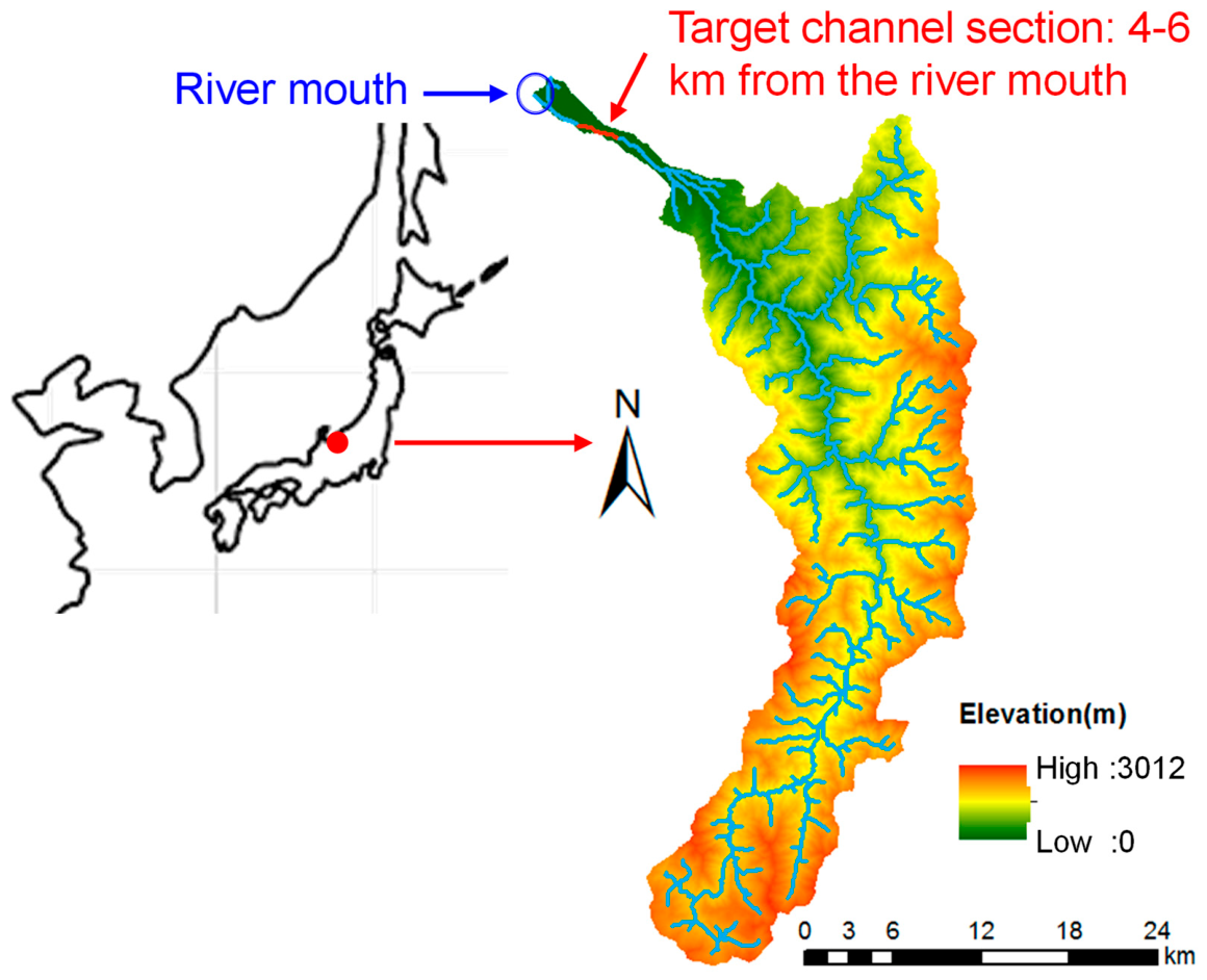
Figure 2.
UAV orthoimage in the target river section of the Kurobe River, 28th November 2017.
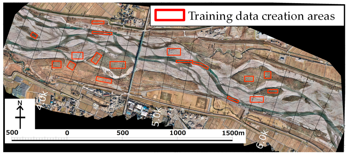
Figure 3.
UAV orthoimage in the target river section of the Kurobe River, 5th November 2018.
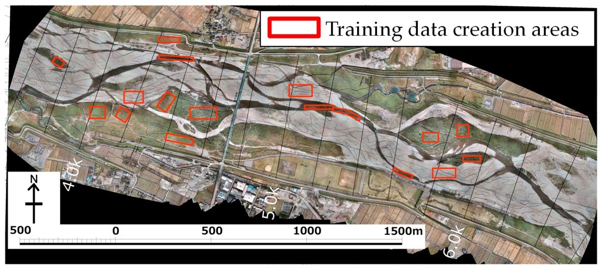
Figure 4.
Satellite image in the target river section of the Kurobe River, 7th November 2017.
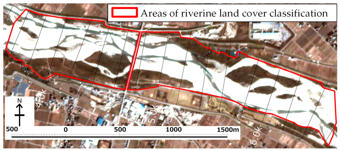
Figure 5.
Satellite image in the target river section of the Kurobe River, 8th November 2018.
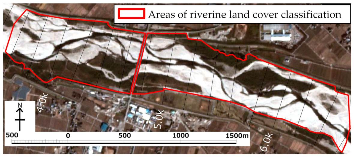
Figure 6.
Flowchart of a machine learning procedure for classifying riverine land covers.
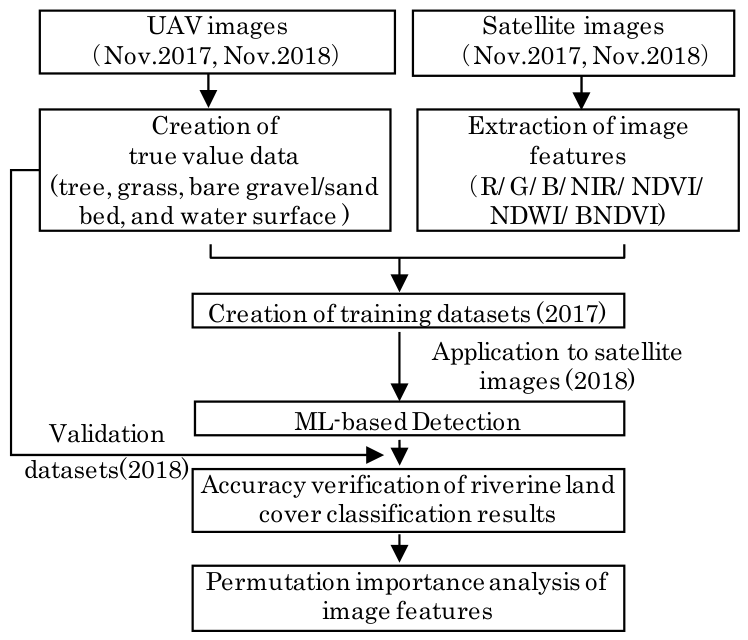
Figure 7.
Histograms of the four bands’ radiance distribution in each image feature obtained from the satellite images.
Figure 7.
Histograms of the four bands’ radiance distribution in each image feature obtained from the satellite images.
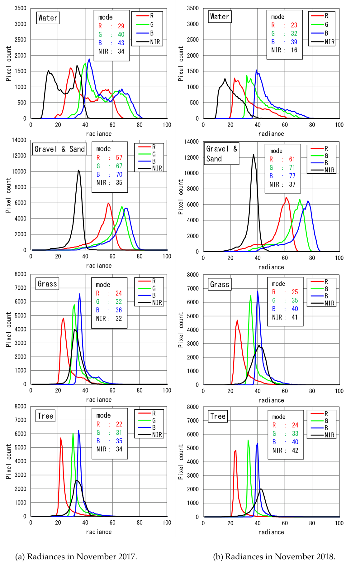
Figure 8.
Histograms of the four normalized indices in each image feature obtained from the satellite images.
Figure 8.
Histograms of the four normalized indices in each image feature obtained from the satellite images.
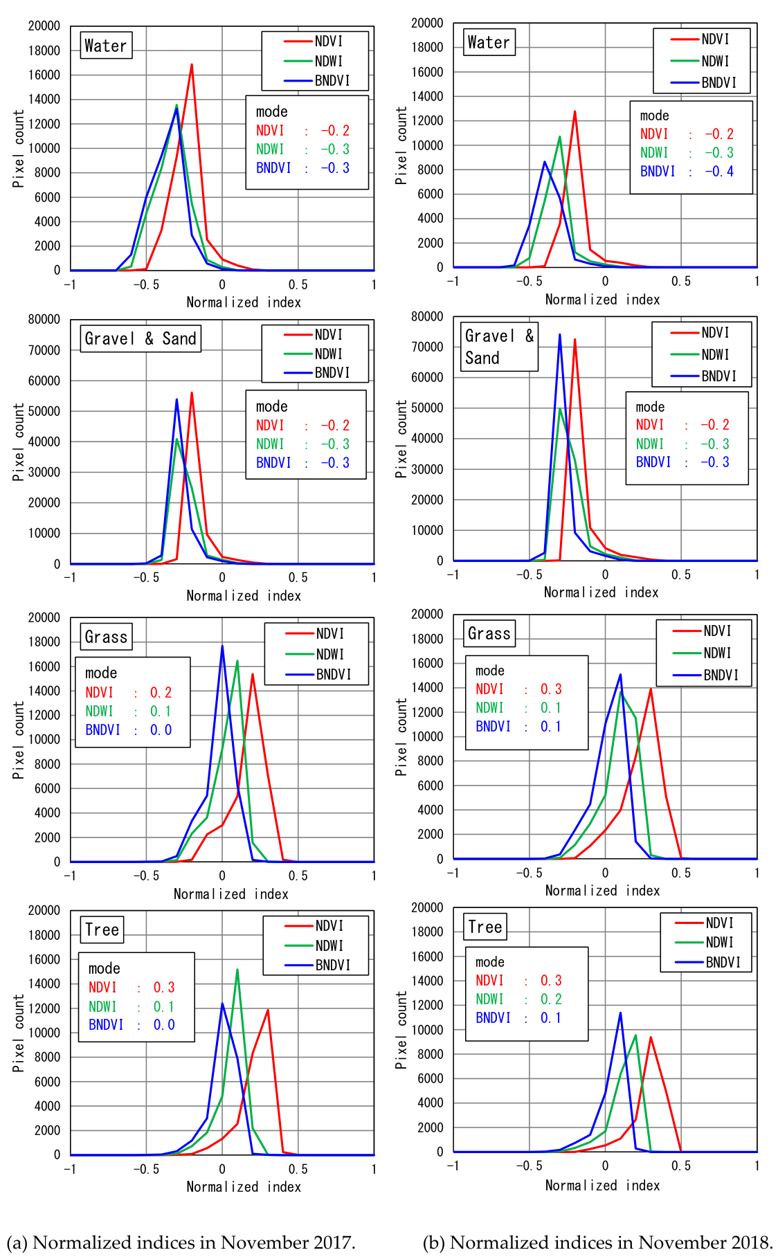
Figure 9.
Distributions of riverine land cover classification by the RF machine learning method for the satellite image in November 2018.
Figure 9.
Distributions of riverine land cover classification by the RF machine learning method for the satellite image in November 2018.
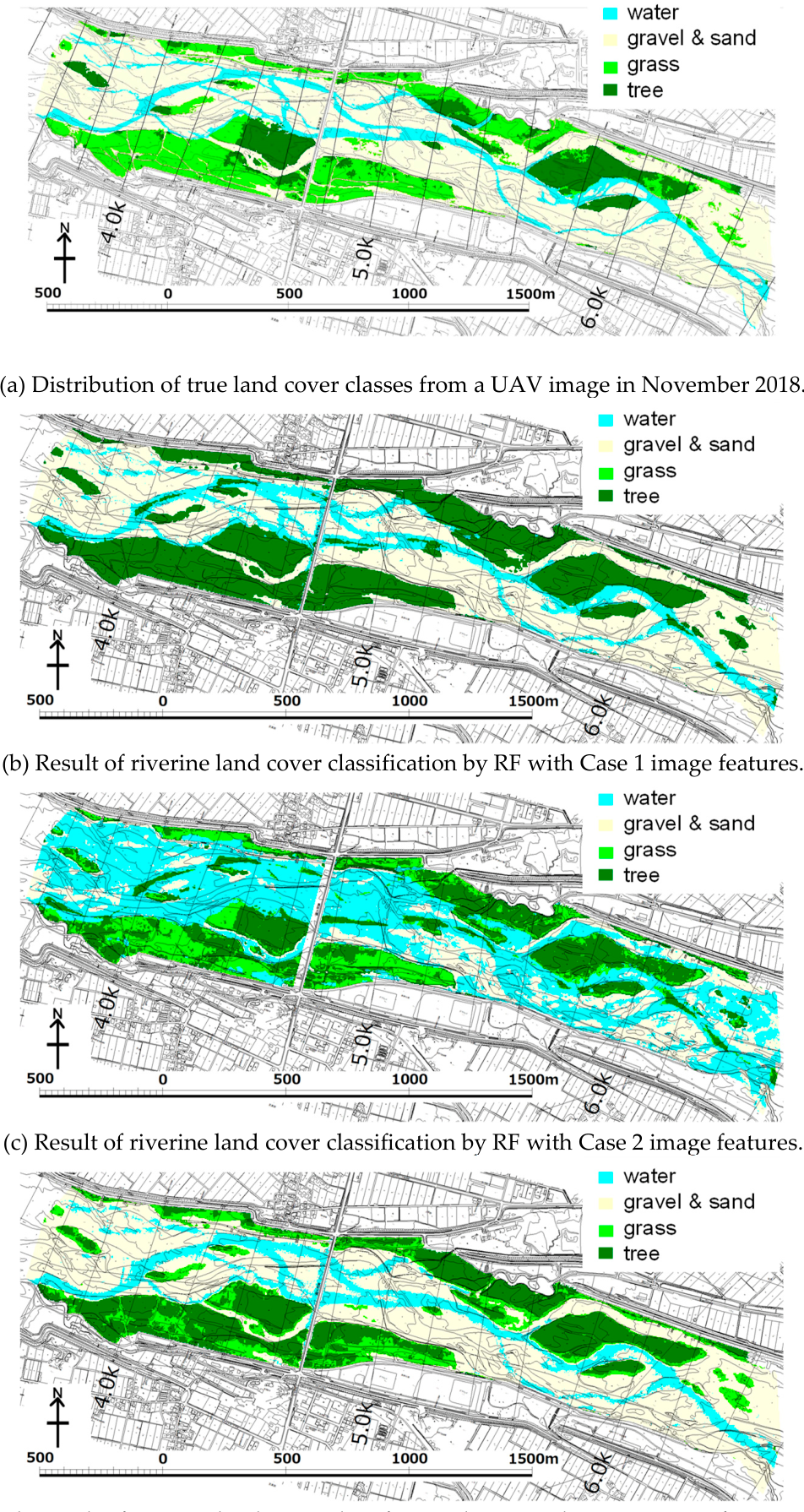
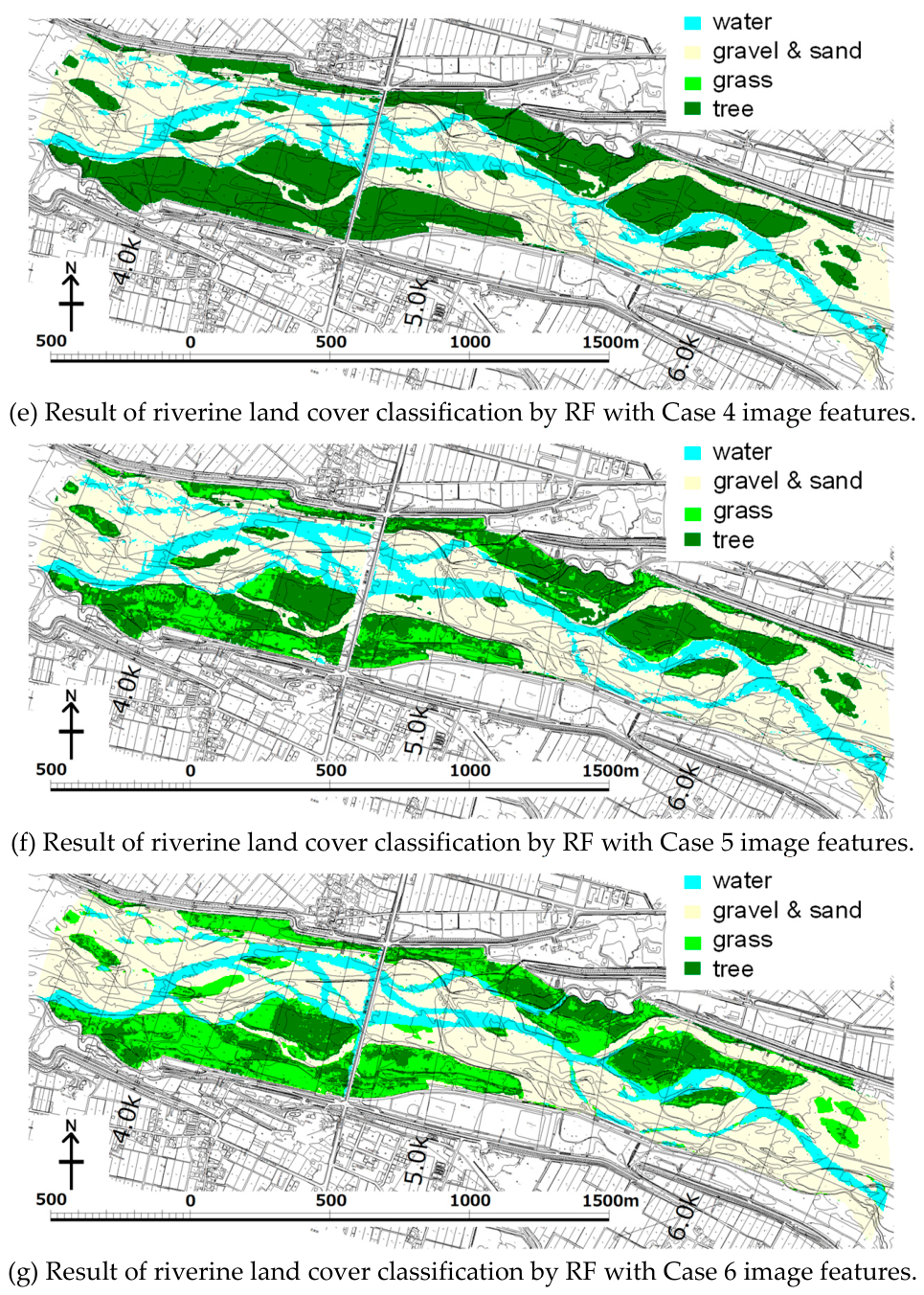
Figure 10.
Permutation importance values of land cover classifications with the datasets of different image features in Cases 1-6, in November 2018.
Figure 10.
Permutation importance values of land cover classifications with the datasets of different image features in Cases 1-6, in November 2018.
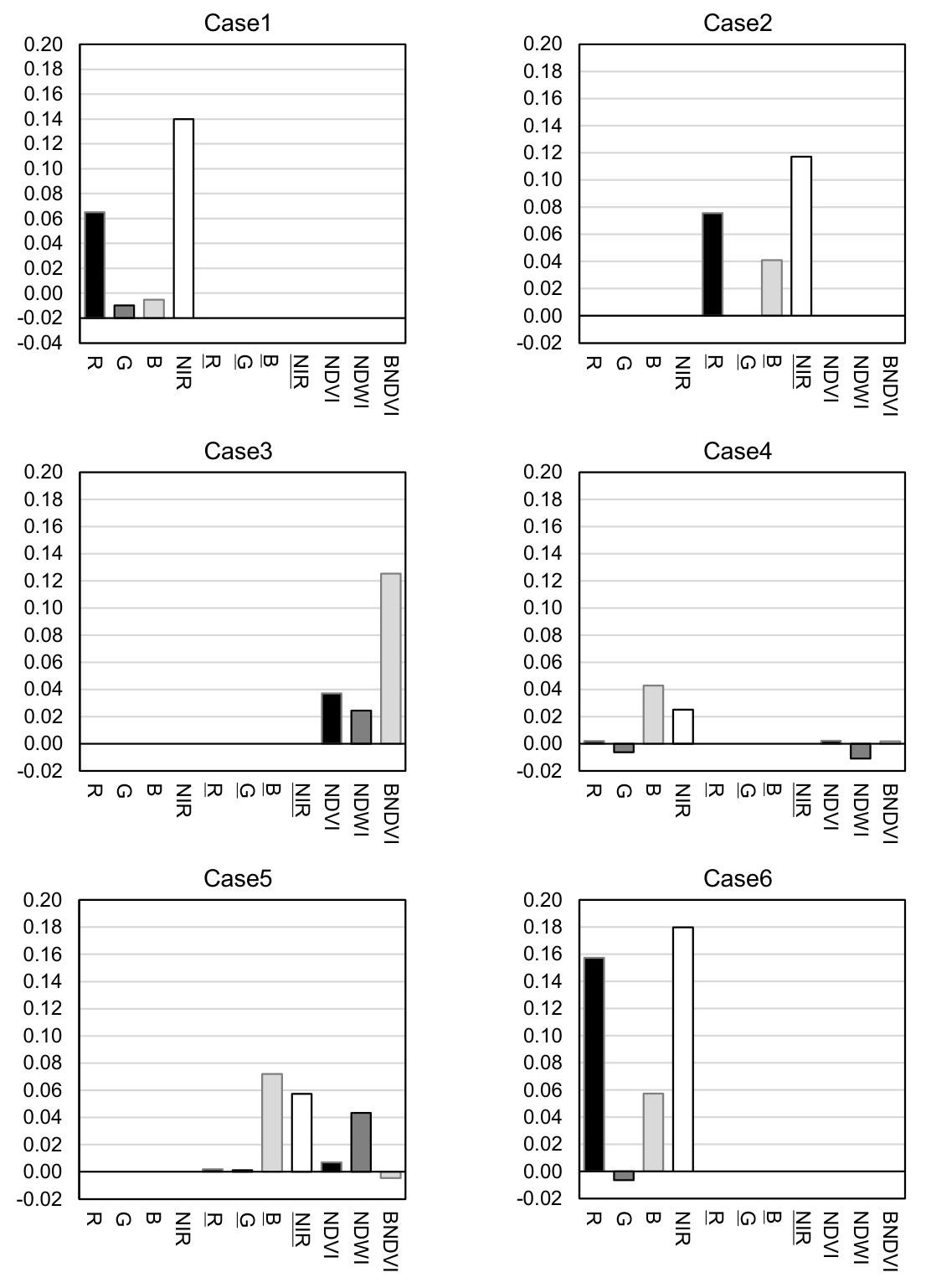

Table 1.
Specification of the satellite and UAV images.
| Item | Satellite imagery | UAV imagery |
| Satellite/Product names | Dove (Planet) | eBee (senseFly) |
| Specification | B/G/R/NIR | B/G/R/NIR/Red edge |
| Spatial resolution | 3.0 m | 0.1 m |
Table 2.
Datasets of image features used for turning the machine learning model.
| Datasets | Case 1 | Case 2 | Case 3 | Case 4 | Case 5 | Case 6 |
| R, G, B, NIR (Obtained from satellite imagery in November 2017.) |
○ | ○ | ○ | |||
|
R, G, B, NIR (Obtained from satellite imagery in November 2017.) |
○ | ○ | ||||
| NDVI, NDWI, BNDVI (Calculated from R, G, B, and NIR in the satellite imagery in November 2017.) |
○ | ○ | ○ | |||
| R, G, B, NIR (Obtained from satellite imagery in November 2018.) |
○ |
Note: R, G, B, and NIR were standardized to the values between -1 and 1 based on the radiance distribution of the target areas.
Table 3.
Comparison of riverine land covers classification accuracy in November 2018 by F-measure.
| Land cover class | F-measure | |||||
|
Case 1 (Fig. 9 (b)) |
Case 2 (Fig. 9 (c)) |
Case 3 (Fig. 9 (d)) |
Case 4 (Fig. 9 (e)) |
Case 5 (Fig. 9 (f)) |
Case 6 (Fig. 9 (g)) |
|
| Water | 0.69 | 0.27 | 0.73 | 0.74 | 0.72 | 0.79 |
| Gravel & Sand | 0.90 | 0.48 | 0.89 | 0.89 | 0.88 | 0.90 |
| Grass | 0.00 | 0.59 | 0.44 | 0.00 | 0.54 | 0.65 |
| Tree | 0.47 | 0.54 | 0.56 | 0.47 | 0.53 | 0.60 |
| All classes | 0.63 | 0.49 | 0.74 | 0.64 | 0.75 | 0.80 |
Disclaimer/Publisher’s Note: The statements, opinions and data contained in all publications are solely those of the individual author(s) and contributor(s) and not of MDPI and/or the editor(s). MDPI and/or the editor(s) disclaim responsibility for any injury to people or property resulting from any ideas, methods, instructions or products referred to in the content. |
© 2026 by the authors. Licensee MDPI, Basel, Switzerland. This article is an open access article distributed under the terms and conditions of the Creative Commons Attribution (CC BY) license (http://creativecommons.org/licenses/by/4.0/).
Copyright: This open access article is published under a Creative Commons CC BY 4.0 license, which permit the free download, distribution, and reuse, provided that the author and preprint are cited in any reuse.


