
Submitted:
21 July 2026
Posted:
22 July 2026
You are already at the latest version
Abstract
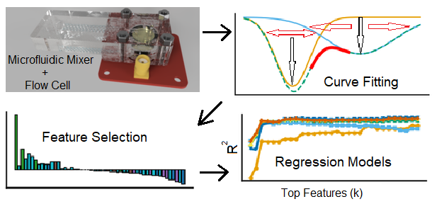
Liquid-phase quartz crystal microbalance (QCM) biosensors are commonly quantified using scalar readouts such as frequency shift, dissipation, or bandwidth. Although these descriptors are useful, they can discard resonance line-shape morphology that contains additional information for quantitative inference. Here, we present a machine-learning-assisted impedance line-shape workflow for temporally robust quantitative 10 MHz QCM biosensing. A passive microfluidic mixer was used to generate controlled glycerol–water concentration gradients under constant total flow while complex impedance spectra were acquired in real time. Each sweep was parameterized using constrained Gaussian/Lorentzian models to obtain 52 physically interpretable descriptors spanning resistance, reactance, impedance magnitude, admittance components, and phase. The pipeline combines consensus outlier handling, training-fold mRMR feature ranking, and regression models evaluated under both corrected shuffled five-fold cross-validation and a stricter temporally blocked validation protocol. The shuffled reference model achieved R2=0.948 and RMSE = 0.162 %v/v, while seven-block temporal validation achieved R2=0.764, RMSE = 0.343 %v/v, and MAE = 0.246 %v/v. Under the same row-matched comparison, a Kanazawa frequency-shift baseline derived from the |Z| trough position yielded R2=0.331, RMSE = 0.578 %v/v, and MAE = 0.416 %v/v. Feature-set ablation further indicated that phase and conductance line-shape descriptors contain particularly strong temporally generalizable information. To demonstrate relevance for recognition-based biosensing, the workflow was also evaluated in an experimental DNA hybridization QCM assay in 1× PBS. Using all replicate-level predictions, the impedance line-shape ML pipeline reduced mean absolute percentage concentration error from 21.02% for conventional Δf calibration to 10.73%, corresponding to a 48.9% reduction in prediction error. These results show that impedance-resolved resonance morphology can improve quantitative QCM biosensing beyond scalar frequency-shift calibration and provides an interpretable basis for AI-assisted electronic biosensors.
Keywords:
quartz crystal microbalance
; QCM biosensors
; AI-assisted biosensing
; impedance spectroscopy
; resonance line-shape analysis
; temporally blocked validation
; interpretable machine learning
; mRMR feature ranking
; Kanazawa baseline
; microfluidic concentration profiling
; DNA hybridization
; concentration prediction
1. Introduction
Quartz crystal microbalance (QCM) sensing offers real-time, label-free transduction and has become a workhorse for probing interfacial processes, adsorption, and viscoelastic films in liquids. In the rigid, thin-film limit, the resonance frequency shift follows Sauerbrey’s gravimetric relation [1]. In liquid-phase operation and for soft or viscoelastic loads, the response reflects coupled inertial, viscous, and elastic contributions; consequently, interpretation relies on hydrodynamic and viscoelastic frameworks such as the Kanazawa–Gordon bulk-loading model [2,3] and layered viscoelastic treatments (e.g., Voinova-type approaches) [4,5], with broader conceptual discussion by Johannsmann [6]. Modern practice and application breadth are summarized in recent QCM/QCM-D and acoustic-wave sensing reviews [7,8,9,10,11,12,13,14].
Despite this strong physical foundation, many workflows still compress rich resonance information to a small set of scalar descriptors, most commonly and a dissipation- or bandwidth-related metric ( or ). Such low-dimensional readouts are attractive for routine use but can be information-limiting for quantitative inference when multiple mechanisms (bulk viscosity/density changes, interfacial slip, viscoelastic relaxation, surface roughness, or mixed-mode loading) produce partially overlapping contributions [6,11,12,15]. Similar limitations arise when viscosity/density effects are inferred from a single closed-form relation (e.g., Kanazawa-type expressions), because the response depends on coupled fluid properties and can be perturbed by real-world experimental conditions; this motivates impedance-resolved, parameter-rich and regression-based inference approaches in complex liquids. [16,17,18]. This creates a clear opportunity for data-driven inference: QCM provides information-rich spectra, but standard readouts collapse them to low-dimensional signals, motivating ML pipelines that exploit the retained spectral structure while preserving physical interpretability.
A direct route to increased information utilization is impedance- (or admittance-) resolved analysis, where the full resonance line shape is acquired and parameterized rather than reduced to two metrics. Prior work has shown that full admittance/impedance spectra contain richer structure than a single frequency shift, and that multivariate analysis of spectral descriptors can separate different physical contributions in liquid-phase QCM measurements [19,20,21,36]. In particular, relating the complete admittance spectrum of a loaded resonator to material and interfacial properties has been shown to enable quantitative inference that is inaccessible to scalar reductions alone [22]. In parallel, electrochemical impedance spectroscopy has seen growing adoption of machine-learning and multivariate approaches for automated and more robust inference in complex settings, spanning impedimetric biosensing and bioanalytical sensing as well as energy-storage prognostics under variable operating regimes [23,24,25,26,27]. These developments motivate transferring similar AI principles—robust preprocessing, redundancy control, and cross-validated model selection—to impedance-resolved QCM line-shape data.
In this work, we develop an impedance-resolved QCM inference framework that exploits full resonance line-shape information rather than reducing measurements to a two-scalar readout. The proposed pipeline is designed around the empirical characteristics of the acquired constant-total-flow dataset: descriptor redundancy is managed using mutual-information–based minimum redundancy maximum relevance (mRMR) ranking with top-k ablations, while transient artifacts and occasional fit failures are mitigated through staged outlier screening and a soft-consensus ensemble filter. To avoid overestimating performance in a time-ordered sinusoidal experiment, we evaluate the corrected pipeline under both shuffled five-fold cross-validation and a stricter temporally blocked protocol in which contiguous portions of the experiment are held out. We also use a row-matched Kanazawa baseline computed from the trough frequency position, so that the physics-based comparator and the learned line-shape model are assessed on the same post-QC sweeps. This framework builds on our group’s prior work on impedance-resolved QCM feature engineering and ML-centric analysis workflows [28,29,30,31,32]. Finally, we extend the analysis to an experimental DNA hybridization QCM assay to demonstrate that the workflow is relevant to recognition-based biosensing and not only to controlled bulk-liquid loading. The remainder of the paper details the experimental/microfluidic setup and spectral parameterization, the feature processing and learning pipeline, the validation strategy, and the comparative results and discussion.
2. Materials and Methods
2.1. Fabrication of Flow Cell with Passive Mixer
2.1.1. CAD/CAM and Machining
The flow cell comprises three layers of 3-mm cast acrylic (PMMA). Geometry and toolpaths were prepared in Autodesk Fusion 360 and milled on an in-house built CNC. Mixer features were cut with a flat end mill inside a 3D-printed water bath for chip removal and thermal control. Unless noted, the feed rate was and spindle speed . All ports, through-holes, and the QCM seat were machined before bonding.
2.1.2. Passive Mixer Geometry
The middle layer contains an array of circular baffles (pillars) to enhance transverse advection. Pillar diameter is ; the gap between adjacent pillars is . The channel height is . These dimensions balance hydraulic resistance with mixing efficiency and respect the end-mill diameter.
2.1.3. QCM Sealing
A 10 MHz plano-convex AT-cut QCM (vendor: openQCM) is sealed between two elastomer O-rings (major/minor radii ) seated in concentric grooves. The crystal is clamped between the fused (top+middle) assembly and the bottom plate, with O-ring compression defining the wetted footprint and preventing bypass flow.
2.1.4. Electrical Interfacing
A custom PCB carries two spring-loaded pogo pins that contact the QCM electrodes from below through clearance holes in the bottom plate and O-ring groove. The PCB mates to a Keysight E4990A via the 16047E fixture.
2.1.5. Thermal Bonding (Heat Fusing)
The top and middle acrylic layers were permanently joined by controlled thermal bonding. To prevent warping under load, a snug MDF jig was CNC-cut to house the acrylic pair; the jig was clamped between flat aluminum plates, and binder clips provided uniform clamping pressure (layout provided in the Supplemental Information). The stack was heated in a box oven with a ramp to 115 °C, held 30 min, then cooled to room temperature under load, yielding a clear, void-free bond.
2.1.6. Final Assembly
The bonded top–middle assembly, QCM, and bottom plate were stacked with the two O-rings and fastened using screws (Figure 1a). The PCB was then attached so the pogo pins engaged the electrodes. Figure 1a shows the assembled flow cell with the passive mixer; Figure 1b shows machined faces of the acrylic layers (top on the left, bottom on the right). The long pieces in Figure 1b correspond to the top and middle layers that were heat-fused. A step-by-step workflow, jig drawings, clamping pattern, and post-bond cleaning are provided in the Supplemental Information Section S.1.
2.2. Flow Setup
Two inlet streams were driven by a dual-channel Elveflow OB1 MK3+ pressure controller equipped with inline flow sensors; each channel was regulated by proportional–integral (PI) feedback to enforce the programmed rates. Channel 1 (DI water) followed a sinusoidal profile between 30 and 50 l/min with a 1 h period. Channel 2 (5% v/v glycerol) was commanded with an equal-amplitude sinusoid phase-shifted by 180°, varying between 0 and 20 l/min. The phase offset maintained a constant total flow of 50 l/min while modulating composition. Maintaining constant total flow is critical because QCM signals are sensitive to flow-induced hydrodynamic loading; fixing the flow rate reduces this source of variability. After merging, the baffle mixer produced a sinusoidal glycerol concentration at the sensor of 0–2% (v/v). All solutions, the flow cell, and the flow sensors were connected using PTFE tubing (inner diameter 1.0 mm, outer diameter 1.5 mm) with polyether ether ketone (PEEK) fittings and adapters to ensure chemical compatibility and low adsorption. For stable operation of the three-port passive mixer (two inlets, one outlet), the OB1 supplied positive pressure at the inlets; when the PI loop required negative gauge pressure to meet a setpoint, an auxiliary vacuum line (via the OB1 vacuum port/external source) was applied to the inlets. The outlet remained at atmospheric pressure and was routed to a waste container, which helped prevent backflow and stabilized the junction while maintaining the programmed waveform. Flow-rate data sampled at 20 Hz were used to compute real-time concentrations and were interpolated to synchronize with the impedance-sweep timestamps. Figure 1c shows the flow setup and components.
2.3. Impedance Measurements and Curve Fittings
2.3.1. Impedance Measurements
Impedance spectra were collected around the fundamental resonance with 1000 points per sweep and no on-instrument averaging. Each resonance feature was acquired in its own narrow moving frequency window, centered on the feature for all measurements except conductance. The window sizes for the respective resonance features are listed in Table 1. Real-time feature tracking and recentering were applied to all peaks/troughs except G using a peak-monitoring routine based on multiple-parabola resonance peak fitting [28]. The conductance peak was instead measured in a fixed 50 kHz window to guarantee that both tails of the line shape remained within the sweep even under slow drift. Fitting-window selection was predefined and feature-specific to preserve both central and wing information of each resonance observable; the complete windows are explicitly reported in Table 1 and representative wing coverage is visible in Figure 2a.
2.3.2. Curve Fittings
Raw impedance data for each parameter was normalized for frequency only for each parameter separately by subtracting the first sweep’s mean and dividing by its standard deviation to retain shifts in frequency in time after fitting. The normalized spectral data were fitted with a two-term Gaussian model, except for the conductance peak, which was fitted with a Lorentzian function with a constant offset. (Equation (1)) given by
where a, b, c, and d are fitted constants. This parameterization yielded a total of 52 fit parameters. Importantly, the two-term Gaussian representation used for non-conductance features is a phenomenological decomposition of a single asymmetric resonance envelope (left-/right-wing dominant components) and is not interpreted as two distinct physical resonances or modal coupling. Fitting was done using lower and upper bounds which were determined by unbounded fitting all 681 sweeps for each parameter and selecting 2nd and 98th percentiles of each fitted coefficient as lower and upper bounds to prevent overfitting (An unbounded fitting example may be found in Supplemental Information Section S.2). Nine fits in with an less than 0.95 were omitted from the dataset. A sample of fitted curves and raw impedance spectra is shown in Figure 2a, and a boxplot of all the values is plotted in Figure 2b.
2.4. Exploratory Data Analysis and Regression Models
2.4.1. Data Set
In constructing the dataset, each non-conductance resonance feature was fitted with a two-term Gaussian model, and a heuristic ordering was applied to the fitted components to ensure consistency across spectra. Specifically, the component with the larger fitted amplitude was designated as Gaussian 1 and its parameters were recorded with the suffix “1,” while the remaining component was designated as Gaussian 2 with the suffix “2.” The parameters from these two Gaussians, collected over all non-conductance features, yielded 48 input variables in total. The conductance peak was fitted separately with a Lorentzian function, and its four parameters were appended to the feature vector, bringing the total to 52 input parameters per one sweep of each spectrum. The supervised target (output) associated with each 52-parameter vector was the corresponding glycerol concentration at the time of acquisition.
2.5. Outlier Removal
Outlier detection aims to identify and eliminate anomalous data points that deviate substantially from the general structure of a dataset. In experimental measurements, such deviations may arise from random noise, instrumentation errors, or uncontrolled environmental factors. However, distinguishing between genuine noise and boundary-region behavior is nontrivial, as excessive filtering may lead to the loss of informative edge cases that represent physically meaningful system limits. Therefore, a balance must be maintained between preserving boundary behaviors and removing spurious noise that could distort downstream statistical or machine-learning analyses.
To establish this balance, the elbow method was employed to determine threshold values for each outlier detection algorithm. By plotting the number of flagged instances against a percentile or sensitivity parameter, the inflection (“elbow”) point reveals a natural transition between stable and unstable classifications. This approach provides an objective and reproducible threshold selection criterion, minimizing arbitrary parameter tuning.
Parameter bounding and omission of low-quality fits () effectively serve as a first-level outlier removal step, ensuring that only statistically reliable curve-fitting results are included in subsequent analyses.
In this study, outliers were handled in two stages. First, curve-fitting quality control (bounded parameterization and omission of low-quality fits, ) ensured that only statistically reliable descriptors entered downstream analysis. Second, multivariate anomaly scores were computed using three complementary detectors (local distance-based outlier factor, Isolation Forest, and Mahalanobis distance with shrinkage covariance). Scores were normalized and combined via a soft-consensus score, and samples exceeding a robust threshold were excluded. Full definitions, hyperparameters, and threshold selection procedures are provided in the Supporting Information (Section S.5).
2.6. Heatmap of Correlations
A correlation heat map was constructed to evaluate pairwise linear relationships among all fitted parameters. Correlation analysis quantifies the degree to which two variables vary together, with Pearson’s correlation coefficient ranging between –1 and +1, indicating the strength and direction of linear association. The heat map provides a compact, visual representation of these interdependencies, facilitating the identification of clusters of parameters that vary in a similar manner or exhibit inverse trends. This step serves both as an exploratory diagnostic to assess data coherence and as a guide for subsequent feature selection and dimensionality-reduction analyses.
2.7. Feature Importance Analysis
To determine the most informative parameters for predicting glycerol concentration, feature-ranking was performed using mutual information (MI)–based minimum-redundancy maximum-relevance (mRMR) analysis. Feature importance quantifies the explanatory contribution of each variable to the target response, helping to identify those parameters that convey the most useful information while minimizing redundancy among correlated features.
The mutual information (MI) between a feature and the target variable Y measures the reduction in uncertainty about Y when is known. Unlike linear correlation coefficients, MI can capture both linear and nonlinear dependencies. It is formally defined as
where is the joint probability density function and and are the corresponding marginals. A higher MI value indicates a stronger statistical dependence between the feature and the target variable.
To ensure that the selected features are not only relevant but also non-redundant, the mRMR algorithm was applied. The mRMR criterion seeks to maximise the relevance of the selected feature subset S to the target variable while minimising mutual information among features within the subset:
This formulation ensures that the resulting subset of parameters carries the maximum possible information about the response variable without duplication of information between features.
In this study, MI was employed as the primary dependency measure within the mRMR framework, as it provides a deeper and more comprehensive assessment of feature relevance than linear correlation metrics. The resulting ranked list of features was subsequently used to evaluate regression model performance as a function of the number of included parameters.
2.8. Regression Modeling
Regression models were employed to quantitatively assess the effectiveness of the extracted and ranked features in predicting glycerol concentration. The objective was to evaluate the predictive utility of impedance line-shape descriptors and the effect of redundancy-aware feature ranking under a consistent cross-validation protocol, rather than to claim a universally optimal model. To provide a balanced view of model interpretability and nonlinear learning capacity, three distinct classes of regression algorithms were considered.
2.8.1. Linear Models
The Lasso and Elastic Net regressions were implemented to evaluate the predictive power of sparse linear representations. Lasso regression imposes an -norm penalty on the regression coefficients, forcing some weights to zero and thereby performing both regularisation and feature selection. Elastic Net combines the and -norm penalties, providing a compromise between the sparsity of Lasso and the stability of Ridge regression. These models serve as interpretable baselines that reveal whether a linear combination of selected Gaussian- and Lorentzian-fit parameters can adequately describe concentration variations.
2.8.2. Operator-Theoretic Model
The Support Vector Regressor (SVR) was used as a kernel-based approach that projects the input space into a higher-dimensional feature space where linear regression is performed within a tolerance margin . SVR is derived from operator theory and optimization principles, where the regression function is constructed by minimizing structural risk rather than empirical error. This formulation allows the model to capture nonlinear trends while maintaining good generalization performance and resistance to overfitting.
2.8.3. Algorithmic Ensemble Models
To further explore nonlinear relationships and variable interactions, ensemble-based tree models were trained, including Random Forest (RF) and Gradient Boosting Regressor (GBR). Random Forest aggregates predictions of multiple decorrelated decision trees to reduce variance and enhance robustness, whereas Gradient Boosting sequentially builds trees that correct the residual errors of the previous ensemble. These algorithmic models provide complementary insights into complex, nonlinear dependencies that may not be captured by purely linear approaches.
Two validation protocols were used. First, a corrected shuffled five-fold cross-validation analysis was performed to quantify within-distribution predictive capacity when training and validation folds are randomly interleaved across the full experiment. Second, a stricter temporally blocked validation was performed by sorting the data by acquisition order and dividing the corrected post-QC dataset into seven contiguous held-out blocks. In each blocked fold, one temporal block was withheld for validation and the remaining blocks were used for training. This protocol tests whether the model can generalize to temporally separated portions of the experiment rather than relying on neighboring sweeps from the same concentration cycle.
All analyses were performed on the same corrected post-QC dataset (N = 647 sweeps), using fixed random seeds for reproducibility. Feature ranking (mRMR-MID) was recomputed within each training fold and then applied to the corresponding held-out fold to reduce information leakage. Models were evaluated using , RMSE, and MAE on validation folds. For the physics-based comparator, a row-matched Kanazawa baseline was recomputed from the trough frequency position, treated as the series-resonance frequency . The water reference was defined as the mean trough frequency of the 10 rows closest to zero flow-derived glycerol concentration; viscosity and density were computed at 21 °C and inverted using a lookup table constrained to the imposed 0–2%v/v concentration range.
2.9. Simulated Resonance Behavior Analysis Using the Butterworth–Van Dyke Equivalent Circuit
To support interpretation of the impedance line-shape descriptors extracted from experimental spectra, we performed an illustrative simulation using the Butterworth–Van Dyke (BvD) equivalent circuit. The BvD model provides a physically grounded representation of a quartz resonator through a motional branch in parallel with the static capacitance . By imposing controlled perturbations in and , the simulation generates corresponding, physically consistent changes in the resonance response (e.g., resonance frequency, conductance, and phase), enabling a direct check of how the fitted Gaussian/Lorentzian descriptor set responds to known circuit-level variations. Importantly, this simulation is used to enhance interpretability of the extracted features and to provide a controlled reference for trend analysis; it is not intended as a comprehensive surrogate for the full experimental loading physics.
Specifically, we simulated the experiment using the crystal parameters , , , and . A sinusoidal loading pattern was emulated by generating a peak-to-peak shift in the phase-angle peak position over one period comprising 100 sweeps. This target shift was achieved by determining sweep-wise and updates through minimization of the peak-position error, using the same real-time peak-tracking routine applied to the experimental data. The same window sizes and data resolution were maintained as in the experimental dataset. and were re-estimated after each round of nine sweeps, covering all troughs and peaks of the studied impedance parameters. The simulated spectra were then processed with the same downstream pipeline (feature extraction and filtering) up to the bivariate analysis stage, enabling like-for-like comparison of descriptor behavior between simulated perturbations and experimental observations.
2.10. Classical Kanazawa Model Based on Impedance
Kanazawa based model predictions are calculated using half-bandwidth, , which for Newtonian fluids shifts equally with , fundamental resonance frequency[10]. The calculations involves peak position and baseline determination of the conductance, and subsequent detection as explained in detail before [31]. The viscosity values calculated from the impedance data was then converted into data oriented concentration as explained before and compared with the actual glycerol concentrations.
2.11. Experimental DNA Hybridization Assay and Concentration-Prediction Analysis
To test whether the same impedance-resolved analysis framework can support a canonical recognition-based biosensing workflow, an experimental DNA hybridization assay was added using a 10 MHz QCM format. Prior to probe immobilization, QCM crystals were cleaned, electrically insulated, and functionalized with (3-Mercaptopropyl)trimethoxysilane (MPTMS) to generate a thiol-presenting surface. The thiolated surface was then reacted with sulfo-SMCC, a heterobifunctional linker containing a maleimide group for coupling to surface thiols and an NHS ester group for subsequent reaction with primary amines [28,33]. After linker activation and rinsing, a 5′-amine-modified capture probe containing a 12C PEG spacer between the terminal amine and the recognition sequence was immobilized on the surface. The capture-probe sequence was 5′-NH2–PEG12–CCTACGCCACAAGCTCCAAC-3′, and the immobilized probe was used to capture the fully complementary single-stranded DNA target, 5′-GTTGGAGCTTGTGGCGTAGG-3′. Unless otherwise stated, probe immobilization was performed by incubating the sulfo-SMCC-activated QCM surface with the amine-modified probe in PBS, followed by rinsing, quenching of residual active ester groups. Target oligonucleotides were prepared by serial dilution in 1× phosphate-buffered saline (PBS) and introduced after a buffer-stabilization period. The time-course experiment was divided into a 0–30 min buffer/control interval followed by target-DNA injection at 30 min and post-spike monitoring until 60 min. The concentration series was analyzed both by conventional frequency-shift calibration and by the impedance line-shape ML pipeline. For the conventional analysis, the final frequency shift was fitted with a Langmuir-type characteristic curve, and concentration uncertainty was estimated from replicate experiments performed within the linear region of the characteristic curve. Three replicate experiments were performed at each concentration. For each replicate, the frequency shift (( f)) was calculated as the average response between 57 and 60 min, after the signal had plateaued. These frequency shifts were then used to predict concentrations from the Langmuir fit. For the ML-pipeline comparison, the same experimental data were used to train and evaluate the ML pipeline. The initial 30 min buffer/control interval of each run was labeled as zero concentration, and the same 3 min plateau interval was labeled with the corresponding target concentration for each DNA injection. The performance of both methods was quantified using the mean absolute percentage error (MAPE).
3. Results and Discussion
3.1. Curve Fitting and Parametric Representation
The impedance spectrum around peak and troughs are not symmetrical as can be seen Figure 2a. In order not to lose this vital information functions retaining important parameters such as peak height, width and position were chosen to fit with high with least amount of parameters. Asymmetry in gaussians require at least 2 terms. Fitting 2 term gaussians caused overfitting as shown in supplemental information, Section S.2. Centers of individual gaussians converge to outlier frequencies for a minimal gain in increase making a pattern with changing with concentration difficult to emerge. To prevent this an unbounded fitting was used to determine boundaries for fit values as described which lowered the values, as can be seen in Figure 2b the lowest value was 0.9743.
Each impedance spectrum was reduced to a compact, physically meaningful set of line-shape descriptors. For all parameters except conductance G, the spectral neighbourhood is modeled with a two-term Gaussian mixture, capturing peak intensity, location, and width while remaining robust to minor asymmetries and baseline drift. The conductance peak, which is theoretically Lorentzian from the BvD model [11], was fitted with a Lorentzian function with constant offset to accommodate the experimentally observed baseline while preserving a compact four-parameter representation. Bounds on fit coefficients were derived from percentile statistics over all sweeps to prevent overfitting and ensure reproducibility. This procedure yields a 52-feature representation per one sweep of each spectrum that preserves the core resonance information in a form suitable for multivariate analysis. We selected Gaussian and Lorentzian parameterizations, although third-order polynomial models also achieved high- fits to the line shape. This choice preserves interpretability by yielding direct descriptors of resonance morphology—peak position, peak amplitude, and width (FWHM-related quantities)—whereas polynomial coefficients are less physically transparent.
Figure 2b summarizes goodness-of-fit across parameters: with the exception of Susceptance, all values exceed 0.995, indicating that the chosen parametric forms closely track the measured spectra. The slightly lower for Susceptance likely reflects its higher noise sensitivity and broader low-curvature region, but residuals remain small and structureless relative to signal magnitude. Combined with the prior exclusion of low-fidelity fits and percentile-based coefficient bounds, these results confirm that the fitted features provide a faithful and stable surrogate of the raw spectra, suitable for downstream correlation analysis, feature ranking, and regression.
3.2. Outlier Detection
3.2.1. Ordering in the Venn Diagram
Figure 3a shows that Isolation Forest (IF) removed the most points (62), Local Distance–Based Outlier Factor (LDOF) fewer (17), and Mahalanobis distance (MD) the fewest (2), with MD a subset of the other two. This ordering is consistent with each method’s sensitivity: IF isolates observations by random partitions and therefore readily flags sparse tails and small peripheral clusters (higher recall); LDOF emphasizes local density contrast and is stricter when a point lies near a cohesive neighborhood (moderate recall); MD assumes an approximately elliptical global structure with shrinkage covariance and typically marks only the most extreme, directionally deviant points (highest precision, lowest count). Hence the empirical pattern , and MD points tend to fall within the sets detected by IF/LDOF.
3.2.2. Soft Consensus Method
None of the above three methods lead to an elbow graph which is an indication that individual outlier detection methods do not catch the boundary behavior (Details may be found in Supplemental Information Section S.5). To obtain a unified decision, a soft consensus ensemble method is employed that fuses continuous anomaly scores rather than binary votes. After robust normalization to a weighted score is computed and an outlier is flagged when (here is the threshold). Because soft consensus aggregates sub-threshold but consistent evidence across detectors, it can identify points that do not appear in any single method’s binary set—hence additional outliers “outside” the Venn diagram. In contrast, hard consensus operates on binary masks only: a union rule (flag if any method flags) maximises recall, while an intersection rule (flag only if all methods agree) maximises precision but may miss borderline cases; neither leverages graded evidence.
3.2.3. Elbow Selection of the Weight Alpha
The weights are parametrized as and . Plotting the number of flagged outliers versus produces a characteristic elbow curve, seen in Figure 3b: large changes in count for small (dominated by IF/MD), followed by a region of diminishing returns as increases (greater emphasis on LDOF’s local-density view). is selected at the elbow—where the slope drops sharply—because it balances noise removal against boundary preservation and yields stable downstream behavior. In our study, this criterion led to .
3.3. Correlations
Figure 4 shows a heat map of the correlation matrix where the matrix has unity diagonal due to perfect self-correlation. When focused around the diagonal, for both the Gaussian terms’ fit parameters and G, all fit parameters are highly correlated. and shows moderate correlation and only the second Gaussian term shows correlation. shows correlation mainly for the fitted center parameter b and the width-related parameter c for both Gaussian terms, and shows the same behavior primarily for the first Gaussian term. The Gaussian c parameter was therefore treated as a width-related descriptor without assigning an independent mechanistic interpretation to individual Gaussian components. Peaks and troughs correspond to the series and parallel resonance frequencies of the Butterworth -Van Dyke equivalent circuit model (BvD).
where . Although, BvD is a simplified model and variations of the BvD model and computational studies on the BvD itself is studied extensively in the literature to better represent the behavior of QCM under load from Newtonian fluids. [11,34,35,36]. As both fs and fp shifts to lower frequencies according to BvD model upon changes in motional inductance () and motional resistance (), due to bulk fluid immersion, more of the parameters were expected to be correlated. Although the asymmetrical impedance peaks were captured fully in simulation as shown in Supplemental Information Section S.3, bivariate analysis of the simulation results of the BvD model shows more of the parameters to be correlated and the pattern of those correlations from stronger to weaker is also different. These results suggest there is a more complicated underlying mechanism in QCM’s response to changes in viscosity of the Newtonian fluid that is not fully captured by the simplified BvD formulation used here, suggesting additional contributions beyond the modeled perturbations. Moreover, although in reality all the peak positions showed high correlation with the concentration with sinusoidal patterns(Figures may be found in Supplemental Information Section S.9), fit parameters in this study captured more nonlinear behavior when combined with regression models predicted the changes in concentration with significantly higher accuracies.
3.4. Parameter Importance
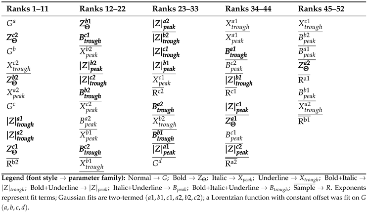
A linear dimensionality analysis of the data set is applied using principal component analysis (PCA). Results may be found in Supplemental Information Section S.6. Table 2 shows the importance of parameters in explaining the variations in the concentration. Other statistical methods to determine parameter information may be found in Supplemental Information Section S.4. The most important parameters is the height of the dissipation peak, followed by the second Gaussian term of the phase angle. Phase angle peak is situated in between the and peaks and as both frequencies shift phase angle peak, shifts. The results indicate the tail of the peak closer to is more responsive to concentration changes. The peak position of the conductance is the third parameter, followed by reactance trough’s second Gaussian term’s width. In the top 10 most important parameters 3 out of 4 terms of the conductance peak is followed by 3 terms of the phase angle covering both of its tails, which is followed by 2 terms of ’s trough both tails’ amplitudes. It is important to note that, the sorting algorithm employed here increases the convergence of the regression algorithm with as little parameters as possible by penalizing unsorted parameters with how redundant they are with respect to already selected parameters in explaining concentration. This means if one has to pick a parameter out of this ranking, a parameter closer to the end may perform quite well alone. (The bar graphs of mRMR-MID scores may be found in Supplemental Information Section S.7)
3.5. Regression Models and Temporally Blocked Validation
To evaluate the predictive value of the fitted line-shape parameters and to verify the benefit of feature selection, Lasso, Elastic Net, SVR, Random Forest, and Gradient Boosting regressors were trained using mRMR-MID-ranked descriptors. Performance was evaluated as a function of the top-k features under two validation protocols (Figure 5). In the corrected shuffled five-fold setting, validation folds contain samples randomly drawn across the full experimental sequence. This protocol measures within-distribution predictive capacity and confirms that the corrected line-shape descriptors support high-accuracy concentration inference; the best shuffled reference model achieved , RMSE = 0.162 %v/v, and MAE = 0.128 %v/v. Regression model results are given in detail for 5-fold CV in Supplemental Information Section S.8. and best performing models’ prediction performances are shown in Supplemental Information Section S.10.
Because the experiment follows a temporally ordered sinusoidal concentration program, a stricter blocked validation was added to test temporal generalization. In this protocol, seven contiguous held-out blocks were used and no neighboring sweeps from the held-out block were available during training. As expected, performance decreased relative to shuffled cross-validation, but the line-shape descriptors retained substantial predictive value. Using the top 30 corrected mRMR-MID descriptors under blocked out-of-fold validation, the proposed model achieved , RMSE = 0.343 %v/v, and MAE = 0.246 %v/v. This result is more conservative than the shuffled five-fold estimate and therefore provides a stronger basis for claiming robustness in time-ordered QCM measurements.
The row-matched Kanazawa comparison provides a physically motivated scalar baseline under the same post-QC sampling. The Kanazawa baseline yielded , RMSE = 0.578 %v/v, and MAE = 0.416 %v/v, whereas the temporally blocked line-shape model reduced RMSE by 40.6% and MAE by 40.8%. The largest line-shape error occurred in the first temporal block, which corresponds to the beginning of the experiment and represents a startup/edge extrapolation case. After this initial block, the blocked model tracked the imposed concentration waveform more closely than the scalar Kanazawa estimate and produced smaller residuals over most of the experimental sequence (Figure 6).
The ablation analysis further clarifies which portions of the impedance line shape carry predictive information (Figure 7). Phase descriptors alone achieved , RMSE = 0.291 %v/v, and MAE = 0.224 %v/v, while conductance descriptors alone achieved , RMSE = 0.319 %v/v, and MAE = 0.223 %v/v. The mRMR top-10 subset achieved and RMSE = 0.332 %v/v, and the proposed top-30 mRMR subset achieved and RMSE = 0.343 %v/v. These results indicate that the gain is not solely due to high-dimensional modeling; rather, specific resonance-morphology descriptors, especially phase and conductance features, provide temporally robust concentration information that is not captured by a single frequency-shift baseline.
3.6. Experimental DNA Hybridization Validation
The glycerol–water experiment establishes that impedance-resolved QCM line-shape descriptors can recover controlled composition changes under constant-flow liquid loading. For biosensor translation, however, the more relevant question is whether the same analysis logic remains useful when the signal originates from a biochemical recognition process. Therefore, an experimental DNA hybridization validation was included as an application-oriented biosensing extension (Figure 8). The time-course data show a stable buffer baseline before target addition and concentration-dependent negative frequency shifts after the DNA spike at 30 min (Figure 8a). The resulting characteristic curve follows a saturating Langmuir-type response, with a fitted apparent of 22.2 nM and a fitted maximum frequency shift of approximately 122 Hz (Figure 8b).
In the actual-versus-predicted concentration analysis, the conventional calibration was compared with the impedance line-shape ML pipeline using all replicate-level predictions rather than concentration-wise means. This distinction is important because error bars reflect replicate variability, and reducing each concentration to a single mean would underestimate the prediction-level uncertainty. Across the plotted concentration range, the conventional method produced a MAPE of 21.02%, whereas the ML pipeline produced a MAPE of 10.73%. This corresponds to a 48.9% reduction in replicate-level concentration-prediction error. The root mean square percentage error was also lower for the ML pipeline (16.62%) than for conventional prediction (29.24%). These results support the central premise of the study: retaining and learning from impedance line-shape morphology can improve quantitative QCM biosensing beyond scalar frequency-shift calibration.
4. Conclusion
Impedance-resolved QCM, integrated with a passive microfluidic mixer and a redundancy-aware machine learning pipeline, was shown to enable temporally robust prediction of small composition changes in the 0– (v/v) glycerol range. By converting each sweep of nine spectra into 52 physically interpretable line-shape features and applying consensus outlier handling followed by training-fold mRMR ranking, the corrected workflow achieved high shuffled five-fold performance (, RMSE = 0.162 %v/v) and retained predictive value under the stricter seven-block temporal validation protocol (, RMSE = 0.343 %v/v). Under the same row-matched comparison, the Kanazawa baseline derived from the trough position yielded and RMSE = 0.578 %v/v. Thus, the temporally blocked line-shape model reduced RMSE by 40.6% relative to the scalar Kanazawa baseline. These results indicate that preserving full resonance morphology–rather than relying only on scalar or endpoints–unlocks robust, information-rich signals for concentration prediction.
The experimental DNA hybridization validation strengthens the biosensing relevance of the workflow by moving the analysis beyond controlled bulk liquid-property inference to a recognition-based QCM assay. In this setting, the impedance line-shape ML pipeline reduced replicate-level MAPE from 21.02% for conventional prediction to 10.73%, corresponding to a 48.9% reduction in concentration-prediction error. This result suggests that impedance-resolved feature extraction can improve concentration estimation in QCM biosensors even when the sensor response is governed by biomolecular binding rather than only Newtonian liquid loading.
From an instrumentation perspective, these findings suggest that QCM workflows constrained to -only endpoints can become an information bottleneck for inference tasks. When prediction accuracy is the primary objective, restricting acquisition and analysis to two scalar readouts may be suboptimal compared with multi-observable, impedance-resolved line-shape processing. The workflow is model-agnostic and hardware-light, making it readily extensible to additional analytes, viscoelastic films, higher overtones, and other piezoelectric resonators, provided that appropriate calibration data are available.
Supplementary Materials
The following supporting information can be downloaded at the website of this paper posted on Preprints.org. Additional experimental details, supplementary figures, and supplementary tables are provided in the supplementary.docx file.
Author Contributions
Conceptualization, C.K. and E.E.; methodology, C.K. and E.E.; software, E.E.; validation, C.K. and E.E.; formal analysis, E.E.; investigation, S.Y.T.; resources, C.K.; data curation, E.E. and S.Y.T.; writing—original draft preparation, C.K.; writing—review and editing, E.E.; visualization, C.K. and E.E.; supervision, C.K. and E.E.; project administration, C.K.; funding acquisition, C.K. All authors have read and agreed to the published version of the manuscript.
Funding
This research was partially funded by the Scientific and Technological Research Council of Türkiye, grant number 122E166.
Data Availability Statement
The raw impedance datasets generated for the glycerol calibration experiments and the analysis codes used for feature extraction, model training, and machine-learning evaluation will be made available in a public GitHub repository upon acceptance. Due to the ongoing nature of the funded project (Grant No. 122E166) and to protect potential intellectual property, the raw time-series files from the DNA-hybridization assay are temporarily restricted. However, the experimental conditions, processed results, and the complete analysis workflow supporting the DNA-hybridization results are fully reported in the article and Supplementary Material to ensure methodological transparency.
Acknowledgments
The authors thank Boğaziçi University Life Sciences and Technologies Application and Research Center for lending the microfluidic pump system.
Conflicts of Interest
The authors declare no conflicts of interest.
References
- Sauerbrey, G. Verwendung von Schwingquarzen zur Wägung dünner Schichten und zur Mikrowägung. Z. Für Phys. 1959, 155, 206–222. [Google Scholar] [CrossRef]
- Kanazawa, K.K.; Gordon, J.G. Frequency of a quartz microbalance in contact with liquid. Anal. Chem. 1985, 57, 1770–1771. [Google Scholar] [CrossRef]
- Kanazawa, K.K.; Gordon, J.G. The oscillation frequency of a quartz resonator in contact with a liquid. Anal. Chim. Acta 1985, 175, 99–105. [Google Scholar] [CrossRef]
- Voinova, M.V.; Rodahl, M.; Jonson, M.; Kasemo, B. Viscoelastic Acoustic Response of Layered Polymer Films at Fluid–Solid Interfaces: Continuum Mechanics Approach. Phys. Scr. 1999, 59, 391–396. [Google Scholar] [CrossRef]
- Voinova, M.V.; Jonson, M.; Kasemo, B. ’Missing mass’ effect in biosensor’s QCM applications. Biosens. Bioelectron. 2002, 17, 835–841. [Google Scholar] [CrossRef] [PubMed]
- Johannsmann, D. Studies of Viscoelasticity with the QCM. In Springer Series on Chemical Sensors and Biosensors; Springer, 2006; Vol. 5, pp. 49–109. [Google Scholar]
- Easley, A.D.; Ma, T.; Eneh, C.I.; Yun, J.; Thakur, R.M.; Lutkenhaus, J.L. A practical guide to quartz crystal microbalance with dissipation monitoring of thin polymer films. J. Polym. Sci. 2022, 60, 1090–1107. [Google Scholar] [CrossRef]
- Tonda-Turo, C.; Carmagnola, I.; Ciardelli, G. Quartz Crystal Microbalance With Dissipation Monitoring: A Powerful Method To Predict the in vivo Behavior of Bioengineered Surfaces. Front. Bioeng. Biotechnol. 2018, 6, 158. [Google Scholar] [CrossRef] [PubMed]
- Songkhla, S.N.; Siraprapa, H.; Thanachayanont, C. Overview of Quartz Crystal Microbalance Behavior for Thin Film Deposition. Chemosensors 2021, 9, 350. [Google Scholar] [CrossRef]
- Johannsmann, D. Studying Soft Interfaces with Shear Waves: Principles and Applications of the Quartz Crystal Microbalance (QCM). Sensors 2021, 21, 7016. [Google Scholar] [CrossRef] [PubMed]
- Arnau, A. A Review of Interface Electronic Systems for AT-cut Quartz Crystal Microbalance Applications in Liquids. Sensors 2008, 8, 370–411. [Google Scholar] [CrossRef] [PubMed]
- Alassi, A.; Benammar, M.; Brett, D.J.L. Quartz Crystal Microbalance Electronic Interfacing Systems: A Review. Sensors 2017, 17, 2799. [Google Scholar] [CrossRef] [PubMed]
- Huang, Y.; Das, P.K.; Bhethanabotla, V.R. Surface Acoustic Waves in Biosensing Applications. Sens. Actuators Rep. 2021, 3, 100041. [Google Scholar] [CrossRef]
- Rocha-Gaso, M.I.; March-Iborra, C.; Montoya-Baides, Á.; Arnau-Vives, A. Surface Generated Acoustic Wave Biosensors for the Detection of Pathogens: A Review. Sensors 2009, 9, 5740–5769. [Google Scholar] [CrossRef] [PubMed]
- Daikhin, L.; Katz, G.; Urbakh, M.; Zagidulin, D.; Borovikov, D.; Filinovskii, V. The Effect of Surface Roughness on the Response of the Quartz Crystal Microbalance in Liquids. Anal. Chem. 2002, 74, 554–561. [Google Scholar]
- Liao, S.; Liu, Z.; Chen, Z.; Zhang, S.; Xu, X.; He, M. Comparing of Frequency Shift and Impedance Analysis Method Based on QCM for Blood Viscosity Measurement. Sensors 2022, 22, 3784. [Google Scholar] [CrossRef] [PubMed]
- Burda, I.; Socoliuc, V.; Chiriac, H. Advanced Impedance Spectroscopy for QCM Sensor in Liquid Medium. Sensors 2022, 22, 2337. [Google Scholar] [CrossRef] [PubMed]
- Voglhuber-Brunnmaier, T.; Nauer, C.; Jakoby, B.; Keplinger, F. Fluid Sensing Using Quartz Tuning Forks—Measurement of Viscosity and Density of Liquids. Sensors 2019, 19, 2336. [Google Scholar] [CrossRef] [PubMed]
- Chen, K.; Tan, Z.; Nie, L.; Yao, S. Principal component analysis applied to admittance spectra of a quartz-crystal microbalance in contact with a liquid phase. Analyst 1995, 120, 1885–1889. [Google Scholar] [CrossRef]
- Buttry, D.A.; Ward, M.D. Measurement of Interfacial Processes at Electrode Surfaces with the Electrochemical Quartz Crystal Microbalance. Chem. Rev. 1992, 92, 1355–1379. [Google Scholar] [CrossRef]
- Deakin, M.R.; Buttry, D.A. Electrochemical Applications of the Quartz Crystal Microbalance. Anal. Chem. 1989, 61, 1147A–1154A. [Google Scholar] [CrossRef]
- Gillissen, J.J.J.; Jackman, J.A.; Tabaei, S.R.; Yoon, B.K.; Cho, N.J. Quartz Crystal Microbalance Model for Quantitatively Probing the Deformation of Adsorbed Particles at Low Surface Coverage. Anal. Chem. 2017, 89, 11711–11718. [Google Scholar] [CrossRef] [PubMed]
- Shimizu, F.M.; de Barros, A.; Braunger, M.L.; Gaal, G.; Riul, A., Jr. Information Visualization and Machine Learning Driven Methods for Impedimetric Biosensing. TrAC Trends Anal. Chem. 2023, 165, 117115. [Google Scholar] [CrossRef]
- Randviir, E.P.; Banks, C.E. A Review of Electrochemical Impedance Spectroscopy for Bioanalytical Sensors. Anal. Methods 2022, 14, 4602–4624. [Google Scholar] [CrossRef]
- Doonyapisut, D.; Orangi, J.; Gooding, R.J.; Shamsi, M.H. Analysis of Electrochemical Impedance Data: Use of Deep Learning for Model Classification and Parameter Estimation. AIChE J. (AIChE Adv.) 2023, 9, e300085. [Google Scholar] [CrossRef]
- Jones, P.K.; Ai, W.; Kukreja, J.S.; et al. Impedance-based forecasting of lithium-ion battery performance amid uneven usage. Cell Rep. Phys. Sci. 2022, 3, 100930. [Google Scholar] [CrossRef]
- Zhang, H.; Sun, Z.; Sun, K.; Liu, Q.; Chu, W.; Fu, L.; Dai, D.; Liang, Z.; Lin, C.T. Electrochemical Impedance Spectroscopy-Based Biosensors for Label-Free Detection of Pathogens. Biosensors 2025, 15, 443. [Google Scholar] [CrossRef] [PubMed]
- Kirimli, C.E.; Shih, W.H.; Shih, W.Y. DNA hybridization detection with 100 zM sensitivity using piezoelectric plate sensors with an improved noise-reduction algorithm. Analyst 2014, 139, 2754–2763. [Google Scholar] [CrossRef] [PubMed]
- Kirimli, C.E.; Elgun, E.; Unal, U. Machine learning approach to optimization of parameters for impedance measurements of Quartz Crystal Microbalance to improve limit of detection. Biosens. Bioelectron. X 2022, 10, 100121. [Google Scholar] [CrossRef]
- Kirimli, C.E.; Elgun, E. Exploratory Data Analysis of Bulk Fluid Viscosity Measurements by Means of Quartz Cyrstal Microbalance Impedance Analysis. In Proceedings of the 2024 International Workshop on Impedance Spectroscopy (IWIS); IEEE, 2024. [Google Scholar]
- Kirimli, C.E.; Elgun, E.; Yuksel, M.M.; Yağmur Tuğtağ, S. An Investigation Into the Impact of Impedance Measurement Parameters on the Limit of Detection of QCM-D Using Machine Learning Model Chaining. IEEE Sens. J. 2025, 25, 5688–5696. [Google Scholar] [CrossRef]
- Kirimli, C.E.; Elgun, E.; Burgun, P.E.; Zorba, O. Kernel-Based Analysis of Impedance Spectroscopy in a Quartz Crystal Microbalance Biosensor. In In Proceedings of the 2025 International Workshop on Impedance Spectroscopy (IWIS), 2025; pp. 13–18. [Google Scholar] [CrossRef]
- Kirimli, C.E.; Shih, W.H.; Shih, W.Y. Specific in situ hepatitis B viral double mutation (HBVDM) detection in urine with 60 copies ml analytical sensitivity in a background of 250-fold wild type without DNA isolation and amplification. Analyst 2015, 140, 1590–1598. [Google Scholar] [CrossRef] [PubMed]
- Martin, S.J.; Granstaff, V.E.; Frye, G.C. Characterization of a Quartz Crystal Microbalance with Simultaneous Mass and Liquid Loading. Anal. Chem. 1991, 63, 2272–2281. [Google Scholar] [CrossRef]
- Muramatsu, H.; Tamiya, E.; Karube, I. Computation of Equivalent Circuit Parameters of Quartz Crystals in Contact with Liquid and Study of Liquid Properties. Anal. Chem. 1988, 60, 2142–2146. [Google Scholar] [CrossRef]
- Huang, X.; Zheng, X.; Ye, Y.; Wang, R.; Wu, D.; Liu, J.; Yuan, G. The Resistance–Amplitude–Frequency Effect of In–Liquid Quartz Crystal Microbalance. Micromachines 2017, 8, 233. [Google Scholar]
Figure 1.
(a) QCM biosensor, Flowcell and Passive mixer. (b) Machined faces of passive mixer. Left: Top layers Right: Bottom layers. (c) Flow setup and experimental components.
Figure 1.
(a) QCM biosensor, Flowcell and Passive mixer. (b) Machined faces of passive mixer. Left: Top layers Right: Bottom layers. (c) Flow setup and experimental components.
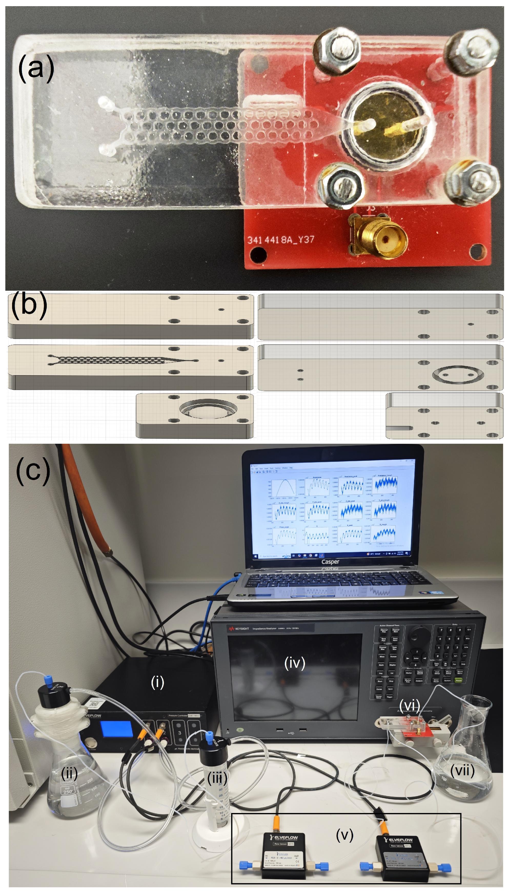
Figure 2.
(a) An example of impedance spectrum around peaks and troughs. (b) Box plots of -values for curve fittings on experimental data giving Impedance spectrum of measurements
Figure 2.
(a) An example of impedance spectrum around peaks and troughs. (b) Box plots of -values for curve fittings on experimental data giving Impedance spectrum of measurements
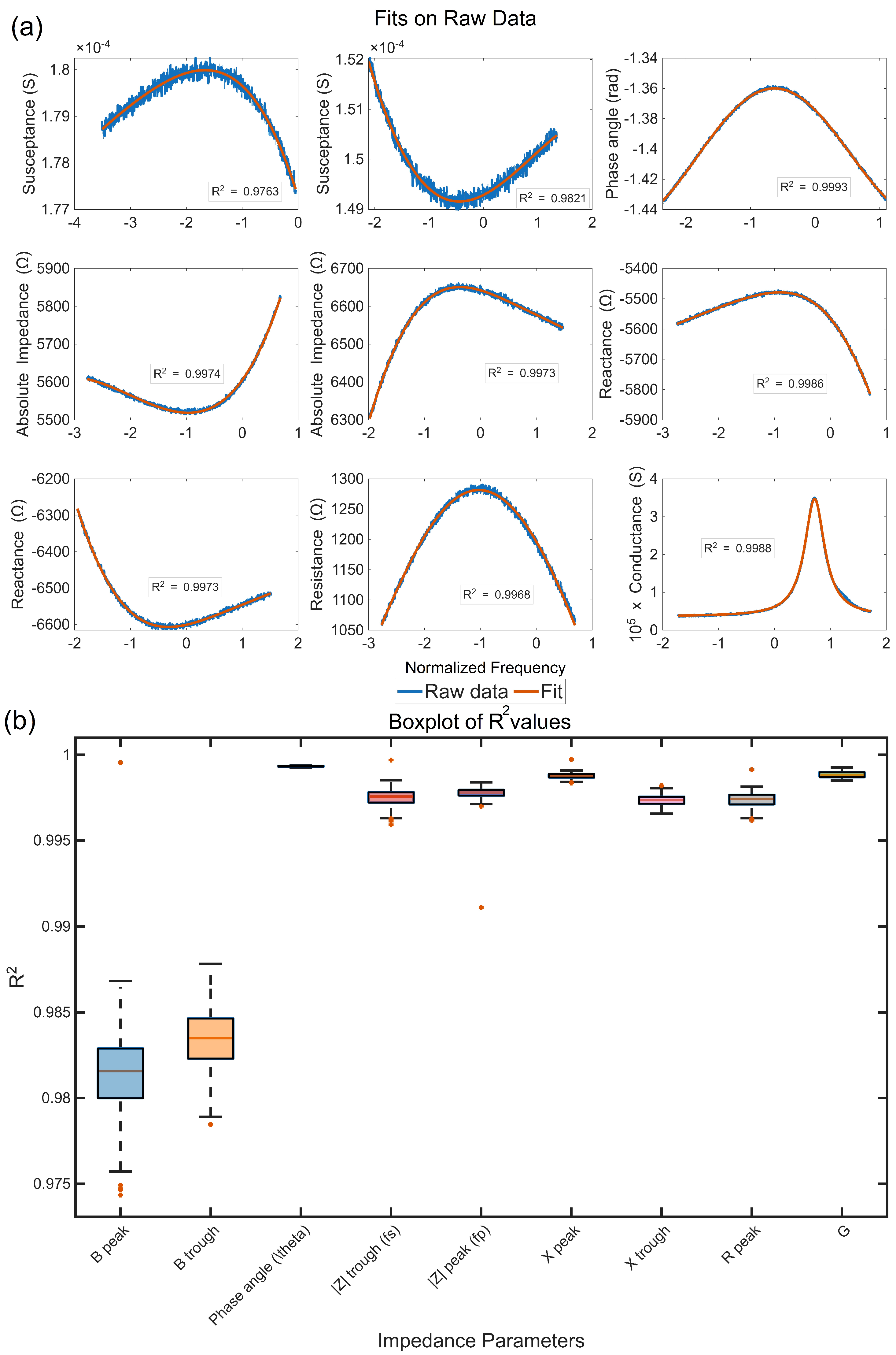
Figure 3.
(a) Venn diagram of outlier points labelled independently by different (LDOF: local distance-based outlier factor, IF: Isolation forest, MD: Mahalanobis distance) algorithms. First number is the number of data points labelled by each method. The number in parentheses denotes the number of those still labelled as outlier by consensus method (b) Graph of number of outliers consensus method sketched with respect to hyperparameter
Figure 3.
(a) Venn diagram of outlier points labelled independently by different (LDOF: local distance-based outlier factor, IF: Isolation forest, MD: Mahalanobis distance) algorithms. First number is the number of data points labelled by each method. The number in parentheses denotes the number of those still labelled as outlier by consensus method (b) Graph of number of outliers consensus method sketched with respect to hyperparameter
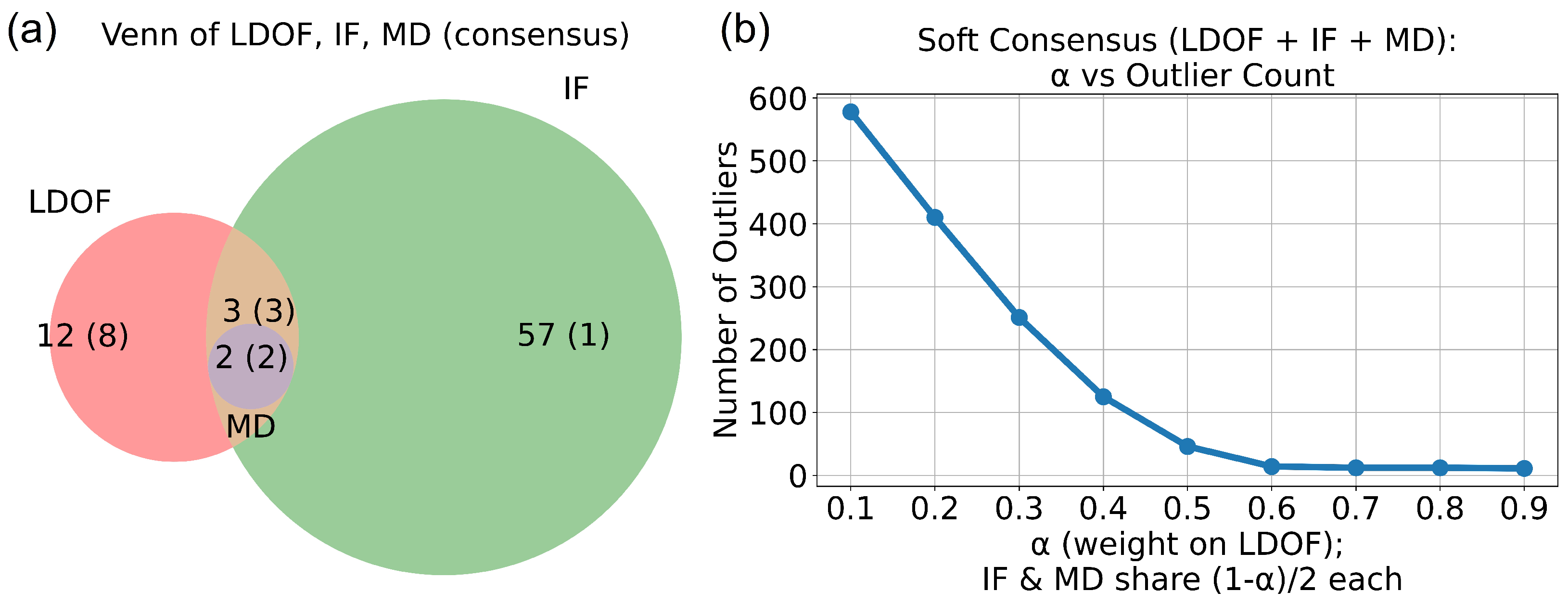
Figure 4.
(a) Heatmap of Pearson correlation values computed for experimental data (b) Heatmap of Pearson correlation computed for BvD simulation results.
Figure 4.
(a) Heatmap of Pearson correlation values computed for experimental data (b) Heatmap of Pearson correlation computed for BvD simulation results.
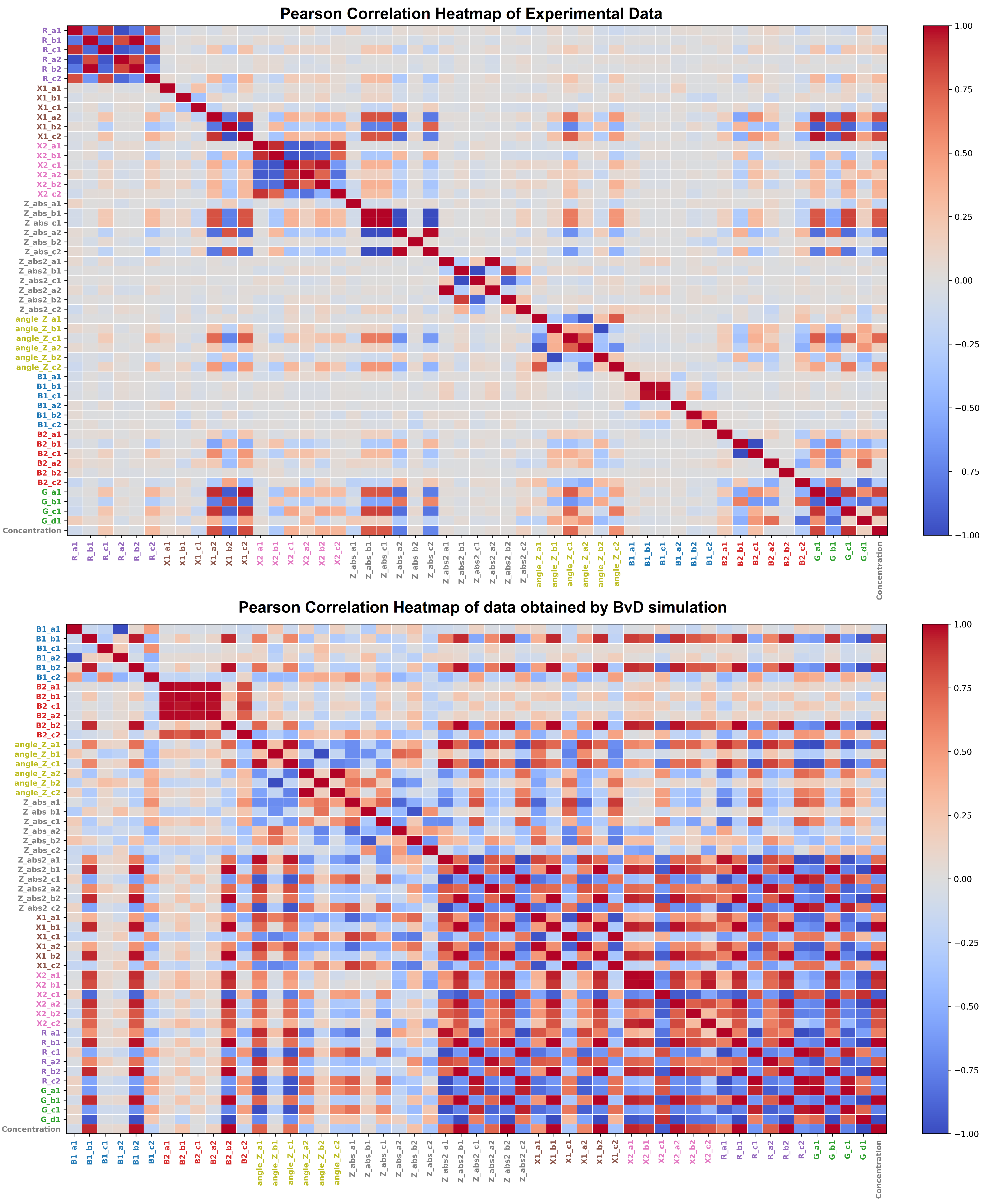
Figure 5.
Corrected model performance under shuffled and temporally blocked validation. (a) Corrected shuffled five-fold cross-validation performance, plotted as validation versus the number of top-ranked mRMR-MID descriptors. (b) Matched blocked/cycle-hold-out validation using the same feature-ranking procedure and model families. The decrease from shuffled to blocked validation quantifies the loss in apparent performance when temporally adjacent sweeps are no longer shared between training and validation folds.
Figure 5.
Corrected model performance under shuffled and temporally blocked validation. (a) Corrected shuffled five-fold cross-validation performance, plotted as validation versus the number of top-ranked mRMR-MID descriptors. (b) Matched blocked/cycle-hold-out validation using the same feature-ranking procedure and model families. The decrease from shuffled to blocked validation quantifies the loss in apparent performance when temporally adjacent sweeps are no longer shared between training and validation folds.
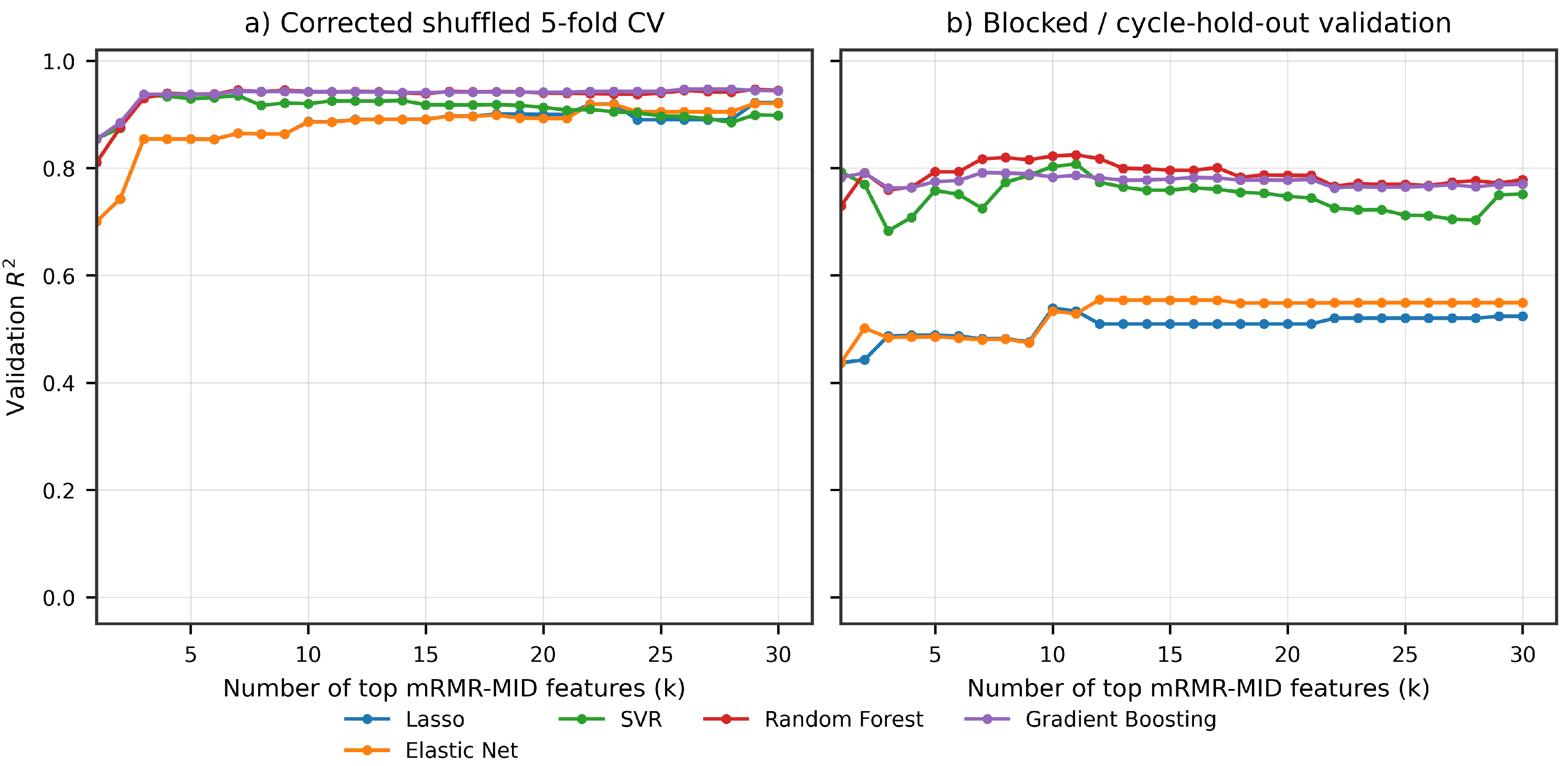
Figure 6.
Temporally blocked out-of-fold validation of impedance line-shape concentration prediction. Seven contiguous temporal blocks were used; in each fold, one block was held out for validation and the remaining blocks were used for training. The model used the top 30 corrected mRMR-MID descriptors. A row-matched Kanazawa baseline was computed from the trough series-resonance frequency position using the mean of the 10 lowest-concentration rows as the water reference, a 21 °C glycerol–water density/viscosity lookup, and a 0–2%v/v inverse concentration grid. The blocked line-shape model achieved , RMSE = 0.343 %v/v, and MAE = 0.246 %v/v, compared with , RMSE = 0.578 %v/v, and MAE = 0.416 %v/v for the row-matched Kanazawa baseline.
Figure 6.
Temporally blocked out-of-fold validation of impedance line-shape concentration prediction. Seven contiguous temporal blocks were used; in each fold, one block was held out for validation and the remaining blocks were used for training. The model used the top 30 corrected mRMR-MID descriptors. A row-matched Kanazawa baseline was computed from the trough series-resonance frequency position using the mean of the 10 lowest-concentration rows as the water reference, a 21 °C glycerol–water density/viscosity lookup, and a 0–2%v/v inverse concentration grid. The blocked line-shape model achieved , RMSE = 0.343 %v/v, and MAE = 0.246 %v/v, compared with , RMSE = 0.578 %v/v, and MAE = 0.416 %v/v for the row-matched Kanazawa baseline.
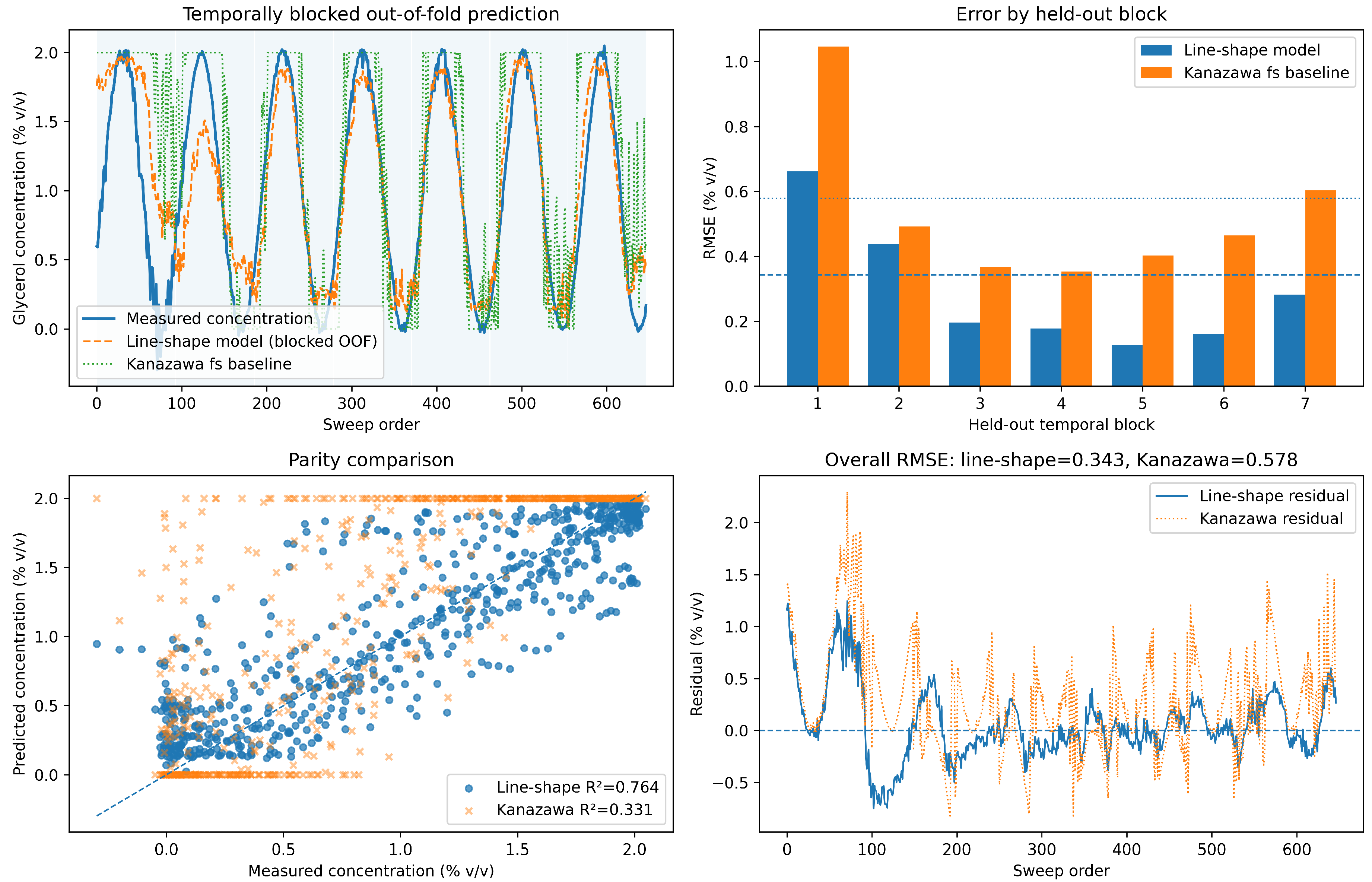
Figure 7.
Feature-set ablation under temporally blocked validation. Restricted descriptor families were compared with the row-matched Kanazawa baseline using the same seven-block out-of-fold protocol. Phase-angle and conductance line-shape descriptors contained particularly strong temporally generalizable information, while compact mRMR-selected subsets and the full 52-descriptor representation remained clearly better than the scalar Kanazawa baseline.
Figure 7.
Feature-set ablation under temporally blocked validation. Restricted descriptor families were compared with the row-matched Kanazawa baseline using the same seven-block out-of-fold protocol. Phase-angle and conductance line-shape descriptors contained particularly strong temporally generalizable information, while compact mRMR-selected subsets and the full 52-descriptor representation remained clearly better than the scalar Kanazawa baseline.
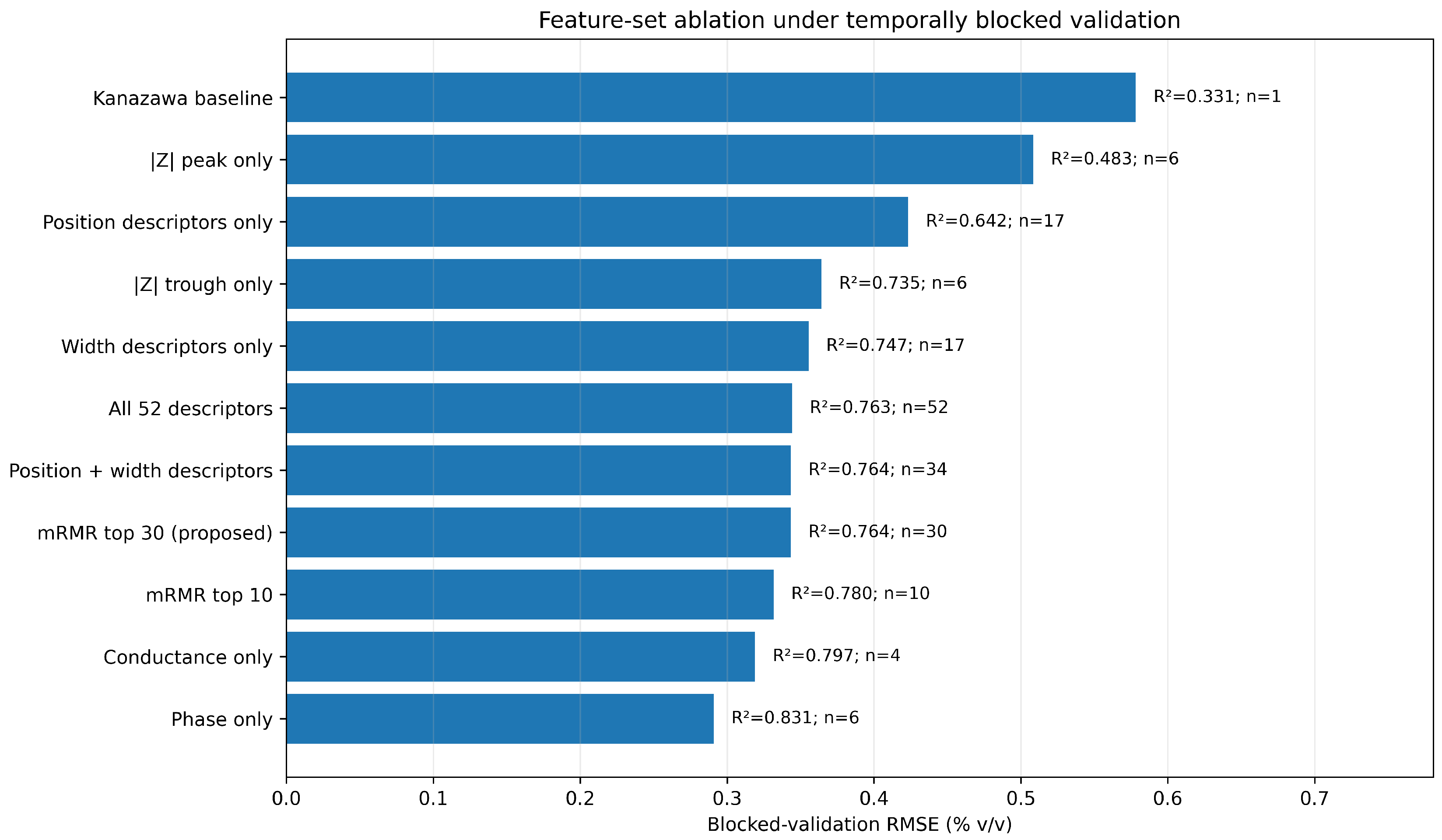
Figure 8.
DNA hybridization QCM biosensing validation of the impedance-resolved ML pipeline. (a) Frequency-shift time courses recorded before and after target-DNA spiking into 1× PBS at increasing complementary oligonucleotide concentrations. Shaded regions indicate replicate variability (). (b) Experimental QCM DNA hybridization characteristic curve fitted with a Langmuir-type model. The LOD threshold was defined as of the buffer/control baseline, and the linear-range cutoff used for conventional -based concentration prediction is indicated. (c) Actual versus predicted concentration obtained using conventional readout and the impedance line-shape ML pipeline. The dashed line indicates ideal prediction (). Prediction errors were evaluated using all replicate-level concentration predictions rather than only the plotted mean values; the displayed ML comparison uses the conservative uncertainty setting corresponding to 50% of the conventional reference uncertainty.
Figure 8.
DNA hybridization QCM biosensing validation of the impedance-resolved ML pipeline. (a) Frequency-shift time courses recorded before and after target-DNA spiking into 1× PBS at increasing complementary oligonucleotide concentrations. Shaded regions indicate replicate variability (). (b) Experimental QCM DNA hybridization characteristic curve fitted with a Langmuir-type model. The LOD threshold was defined as of the buffer/control baseline, and the linear-range cutoff used for conventional -based concentration prediction is indicated. (c) Actual versus predicted concentration obtained using conventional readout and the impedance line-shape ML pipeline. The dashed line indicates ideal prediction (). Prediction errors were evaluated using all replicate-level concentration predictions rather than only the plotted mean values; the displayed ML comparison uses the conservative uncertainty setting corresponding to 50% of the conventional reference uncertainty.
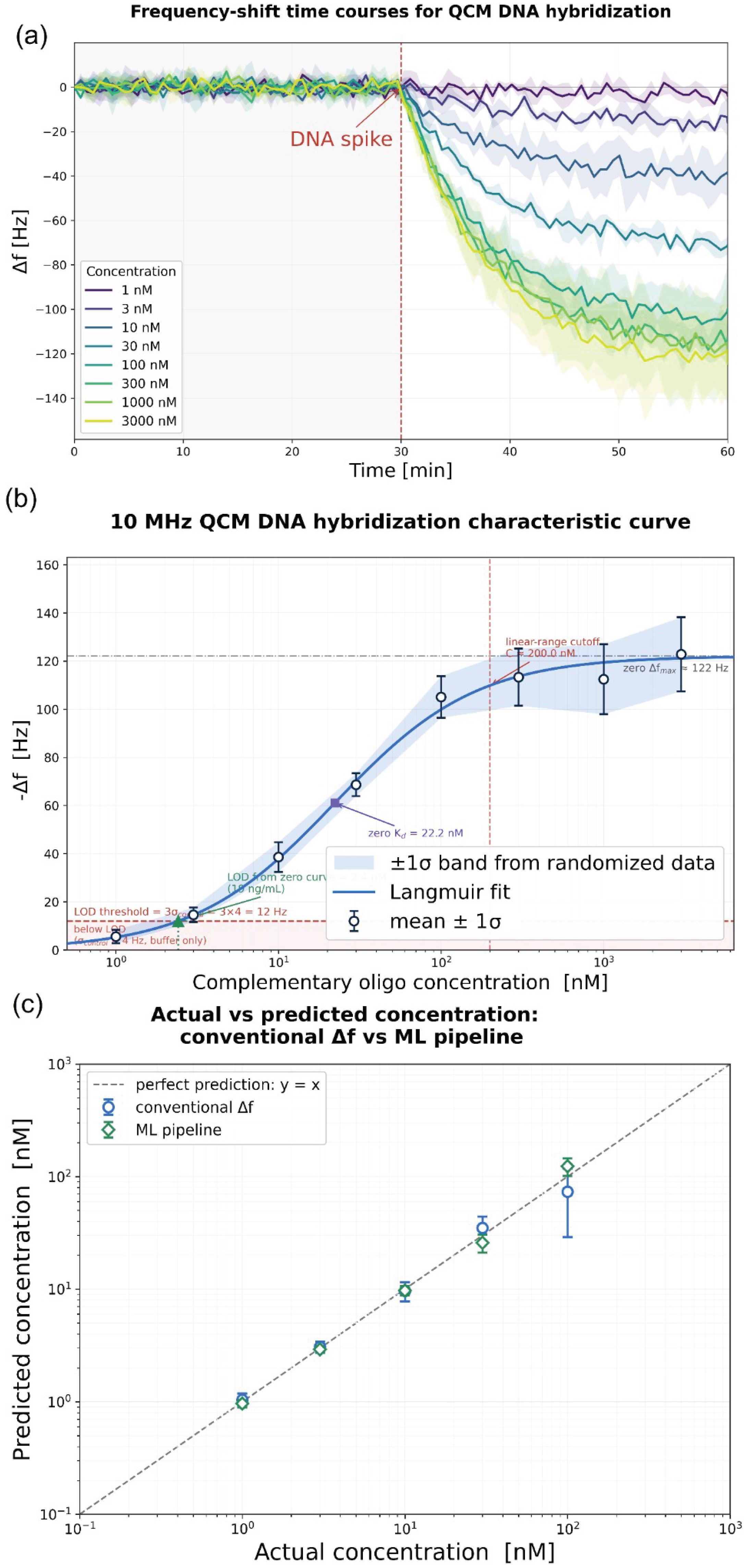

Table 1.
Resonance features and sweep windows (1000 points, no averaging).
| Feature | Window Size | Center Frequency |
|---|---|---|
| 3 kHz | 10008449 | |
| 3 kHz | 10014600 | |
| 5 kHz | 10011947 | |
| 5 kHz | 10008836 | |
| 5 kHz | 10015060 | |
| 5 kHz | 10009210 | |
| 5 kHz | 10015444 | |
| R | 3 kHz | 10012285 |
| G | 50 kHz | 10011585 |
Table 2.
Rank-sorted fit parameters. Columns indicate contiguous rank ranges; rank increases top-to-bottom within each column and then continues in the next column.
Table 2.
Rank-sorted fit parameters. Columns indicate contiguous rank ranges; rank increases top-to-bottom within each column and then continues in the next column.
 |
Disclaimer/Publisher’s Note: The statements, opinions and data contained in all publications are solely those of the individual author(s) and contributor(s) and not of MDPI and/or the editor(s). MDPI and/or the editor(s) disclaim responsibility for any injury to people or property resulting from any ideas, methods, instructions or products referred to in the content. |
© 2026 by the authors. Licensee MDPI, Basel, Switzerland. This article is an open access article distributed under the terms and conditions of the Creative Commons Attribution (CC BY) license (http://creativecommons.org/licenses/by/4.0/).
Copyright: This open access article is published under a Creative Commons CC BY 4.0 license, which permit the free download, distribution, and reuse, provided that the author and preprint are cited in any reuse.


