
Submitted:
20 July 2026
Posted:
22 July 2026
You are already at the latest version
Abstract
Urban road networks in sub-Saharan Africa diverge from traditional sensor-rich, lane-disciplined environments. This paper established an empirical baseline assessment of network efficiency and velocity decay along the 8.0km Mile 17 to Governor's Roundabout corridor (8.0 km) in Buea, Cameroon. Characterized by radial geometry, a steep 25 m/km inbound gradient, unsignalized intersections, and a high mix informal transport (taxis comprising 59.5% and 65.27 of traffic for inbound and outbound flow, respectively). Fifteen-minute Passenger Car Unit (PCU) volume counts were recorded at three measurement points evaluated across three peak windows (morning, afternoon, and evening) over three consecutive weekday observation days. Volume-to-capacity ratios (v/c), peak-hour factors (PHF), equivalent hourly flow rates, space-mean speeds, and Mean Travel Time Indices (MTTI) were calculated for both inbound and outbound flow directions. Results reveal near-saturation and over-saturation at the Bonduma mid-corridor point during morning and afternoon peaks (v/c: 0.98 to 1.06). The highest operational stress occurred during the afternoon outbound window, where over-capacity conditions emerged simultaneously at Mile 17 and Bonduma. MTTI values ranged from 1.36 to 2.04, indicating that congestion is primarily driven by informal transport dynamics rather than absolute vehicle volume. Finally, the paper introduces the Directional Flow Asymmetry Index (DFAI) and Corridor Velocity Decay Rate (CVDR) to successfully quantify critical directional imbalances that traditional aggregate v/c analysis fails to resolve.
Keywords:
network efficiency
; velocity decay
; asymmetric urban corridor
; empirical baseline
; informal transport dynamics
; traffic congestion metrics
; Sub-Saharan Africa transport
1. Introduction
Urban traffic congestion is among the most studied problems in transportation engineering, yet most of the literature focuses on cities with functioning sensor infrastructure, lane discipline, and formal transit systems. In 2022, London recorded 156 hours of per-capita delay to traffic congestion; in the same year, U.S. drivers lost an average of USD 869 per person to congestion-related fuel consumption and time loss [1]. These figures are widely cited. Congestion in mid-size African cities, by contrast, receives far less systemic research attention, despite operational conditions that are structurally distinct from the assumptions embedded in standard traffic models.
Cities across SSA face a structural measurement problem. Standard traffic models assume that vehicles maintain lane discipline, that intersection counts are available from fixed sensors, and that signal timing can be optimized against a known demand profile. In Buea, Cameroon, none of these conditions holds. Taxis stop mid-block without a designated bay; intersections are unsignalized and managed by traffic police during peak hours; and no fixed vehicle detectors are present in the principal corridor. Rwakarehe [2] identifies the absence of corridor-level field data as the primary barrier to effective, localized transport planning in SSA cities.
Reinforcement learning (RL)-based traffic signal controllers have demonstrated significant performance improvements in structured environments. Park et al. [3] showed Deep Q-Network (DQN) controllers reduced delays by up to 22% relative to fixed-time signals in simulation; Almomany et al. [4] extended this to large-scale, multi-agent coordination with real-time CO2 reductions. However, these systems were trained and deployed in environments with structured vehicle classes and sensor feedback. Shuvo [5] notes that widely used simulators such as SUMO, PTV Vissim, and CITY-Flow lack native representations of on-street parking, frequent bus stops, and unregulated mid-block stops, thereby introducing micro-friction that degrades segment capacity. Without field data calculated to local conditions, an RL controller trained on these simulators will systematically misestimate the environment it is meant to serve.
This study addresses the calibration gap for Buea’s principal urban corridor. Three objectives define the work:
- establish an empirical baseline of corridor-level network efficiency and velocity decay for the Mile 17 to Governor’s Roundabout corridor, covering inbound (IB) and outbound (OB) flow across morning, afternoon, and evening peak windows;
- Quantify the directional flow asymmetry using the proposed Directional Flow Asymmetry Index (DFAI) and Corridor Velocity Decay Rate (CVDR); and
- Evaluate the Informal Traffic Disruption Factor (ITDF), laying the groundwork for the Buea Asymmetric Corridor Adaptive Traffic Control (BACATC) reinforcement learning framework.
2. Related Works
2.1. Traffic Flow in SSA Urban Corridors
Research on urban traffic in Sub-Saharan Africa (SSA) has increased significantly since 2021, driven by inter-state data-sharing initiatives and the growing challenges of congestion in secondary cities. Despite this expansion, the literature remains concentrated on a small number of large capital cities such as Accra, Addis Ababa, Lagos, and Nairobi, employing methodologies appropriate to environments with established sensor networks and formal lane discipline.
Rwakarehe, [2] identifies a critical mismatch in transport planning for sub-Saharan African cities, noting that despite a low private car modal share (8%) compared to developed nations, traffic congestion is disproportionately worse, highlighting a clear gap in how standard technical and policy frameworks capture the region’s unique traffic behavior. Chukwurah et al. [6] confirmed for the Enugu arterials in Nigeria, where a week-long traffic census documented a daily mean flow of 2,334 vehicles/h across major distributors, with Abakpa/Nike Road experiencing the highest congestion levels (mean of 809.2 vehicles/h; PHF = 0.79). Statistical analysis confirmed significant spatiotemporal variations (), revealing a non-linear relationship between modest traffic volume increases and severe evening gridlock, attributing these intense localized bottlenecks to complex network dynamics, localized activity patterns, and socio-political factors such as the regional Monday “sit-at-home” orders, which disproportionately amplify Tuesday traffic volumes.
A study of selected intersections in Addis Ababa [7] found that delays were driven not only by traffic volume but by intersection design geometries and pedestrian-vehicle conflict, a condition analogous to Mile 17 node in Buea. Odiakose and Iyeke [8] explicitly noted that bidirectional intersections during the morning peak impacted inbound capacity on the Asaba corridor but could not be quantified because simultaneous bidirectional counts were not collected. The DFAI proposed in the present study directly addresses this gap.
2.2. Informal Transport Modelling
The modelling treatment of paratransit, shared taxis, minibus (clando), and motorcycle taxis (keke), remains one of the major unresolved transport problems in African transport research, due to the mismatch between standard traffic engineering assumptions and local operational realities. Giliomee et al. [9] demonstrated this using SUMO to study electric car and minibus taxis in Cape Town, finding the simulator overestimated energy expenditure by 14% per kilometer and 46% per trip compared to high-quality GPS data, attributing the gap to the simulator’s inability to represent irregular stop-and-go paratransit behavior. According to Behrens and Bruun [10], a successful public transport reform strategy should consider a hybrid network that includes paratransit services. Ackaah [11] explored the implementation of Advanced Traveler Information Systems (ATIS) to manage traffic congestion in developing countries. The study highlights that traffic disruptions in these environments are heavily influenced by structural issues, such as pedestrians being forced to share the same road space with vehicles due to a lack of proper infrastructure. Rather than mathematically modeling volume delay functions, the paper emphasizes practical, low-cost data collection alternatives, such as leveraging Floating Car Data (FCD) from transit fleets like taxis or crowdsourcing speed data via mobile applications, to optimize the existing road network.
2.3. AI Traffic Control in Low-Resource Contexts
Reinforcement learning-based traffic control has attracted substantial research attention since 2021. Park et al. [3] demonstrated that AI agents such as DQN and PPO can reduce traffic delays by up to 22% relative to fixed-time traffic signals and achieve real-time CO2 reduction in a large urban network. Almomany et al. [4] proposed a reinforcement learning-enhanced framework for real-time traffic signal optimization, demonstrating that deploying adaptive algorithms on custom FPGA hardware architectures can achieve a 7 times speedup over modern processing units. Tested within the framework of Kuwait City, their approach addresses critical real-time latency demands while simultaneously lowering fuel consumption and vehicle emissions.
A 2025 survey in the infrastructure literature [12] documents RL-based signal control deployments across dozens of intersections in North America, East Asia, and the Gulf states. Mei et al. [13] identified a core obstacle for low-resource contexts. RL approaches depend on full observation of traffic conditions, but in cities with informal transport and no fixed sensors, corridor behavior observations are sparse or absent. Shuvo [5] made this limitation more explicit by clearly demonstrating that the three simulation environments most frequently deployed to train RL traffic controllers, such as SUMO, PTV Vissim, and CityFlow, by default, operate on rigid lane-based configurations that cannot simulate mid-block stops generated by a 59.4% taxi model share. Bao et al. [14] proposed a federated reinforcement learning (FRL) approach for traffic signal control (TSC), a framework that reduces data transmission requirements, attractive for infrastructure-constrained SSA contexts, but the framework remains vulnerable to systematic error if local nodes are trained on informal traffic streams that the model environment does not represent.
2.4. Study Gap
No corridor-level empirical study of network efficiency, directional flow asymmetry, or velocity decay rates has been identified in the literature for Buea or for comparable secondary cities in Cameroon. While existing studies provide valuable theoretical frameworks, they do not deliver actionable calibration data for a corridor characterized by 59.55% and 65.27% taxi share for inbound and outbound directions, respectively, steep topographic gradients, and asymmetric flow patterns. The field dataset generated by this research represents a novel empirical contribution and directly enables the BACATC framework development in a subsequent phase, shifting the focus from generalized regional patterns to a more localized approach to algorithmic calibration.
3. Theoretical Framework
3.1. Macroscopic Traffic Flow Foundations
All analysis proceeds from the fundamental traffic flow identity [8,15]:
where q (veh/h) is volumetric flow, k (veh/km) is traffic density, and u (km/h) is space-mean speed. Alternative speed–density formulations exist — notably Underwood’s exponential model [17], for the speed–density relationship, the Greenshields linear model [16] is adopted as the primary calibration tool:
where uf is free-flow speed, and kj is jam density. Travel time on congested interrupted-flow corridors is estimated using the Bureau of Public Roads (BPR) volume-delay function [18].
3.2. Network Efficiency Metrics
Ten metrics characterize corridor performance, selected because they can be measured without fixed sensors and are consistent with the IEEE ITS framework [19] and the Highway Capacity Manual (HCM) [20]. Table I summarizes the complete set.

Table 1.
Network Efficiency Metrics.
| No. | Metric | Formula | Category | Reference |
|---|---|---|---|---|
| 1 | Volume-to-Capacity Ratio (v/c) | v/c = q/c | Network Saturation / LOS | [20] |
| 2 | Network Efficiency Index (NEI) | NEI = uobs / uf ∈ [0, 1] | Mobility Performance | [21] |
| 3 | Velocity Decay Coefficient (β) | u = uf(1 − k/kj) | Velocity–Density Sensitivity | [16] |
| 4 | Directional Flow Asymmetry Index (DFAI) | DFAI = (qin − qout) / qmax ∈ [−1, +1] | Flow Balance / Asymmetry | Proposed |
| 5 | Informal Transport Disruption Factor (ITDF) | ITDF = MTTRobs − BPR(VCR) | Informal-Mode Impact | [11,18] |
| 6 | Network Throughput Efficiency (NTE) | NTE = Σ(qi·Li) / Σ(ci·Li) ∈ [0, 1] | System-Level Output | [19] |
| 7 | Mean Travel Time Ratio (MTTR) | MTTR = Tobs/Tff = uf/uobs (min) | Congestion Indicator | [20] |
| 8 | Corridor Velocity Decay Rate (CVDR) | CVDR = (uf − uobs)/uf = 1 − NEI ∈ [0, 1] | Performance Degradation | Proposed |
| 9 | Network Accumulation Index (NAI) | NAI = n(t) / ncrit | MFD Saturation Ratio | [22] |
| 10 | Spatial Congestion Propagation Index (SCPI) | SCPI = ΣLcong / Ltotal ∈ [0, 1] | Congestion Spread | [1,19] |
4. Materials and Methods
4.1. Study Area
Buea is the administrative capital of the South-West Region in Cameroon, with an area of approximately 870 km2. Its population grew from roughly 46,000 in 2000 to over 300,000 by 2022 [23], a growth that the existing road infrastructure was not built to accommodate. The city hosts several major institutions, most notably the University of Buea, the largest Anglophone University in Cameroon, whose access roads feed directly into the study corridor, generating heavy pedestrian-vehicle conflict and demand spikes at the start and end of classes in the morning and afternoon, respectively. The transport system is dominated by taxis (59.55% and 65.27% for inbound and outbound directions of vehicular flow) and minibus operators (clandos), with no functional traffic signals at any of the corridors, approximately fifteen intersections. Traffic police manage peak-period flow manually.
Mount Cameroon’s eastern flank defines the physical topology of the corridor. Road gradients along the study segment range from 4% to 12%, with localized sections exceeding 15% near the Great Soppo area. This sustained elevation gain of approximately 25 m/km in the inbound direction imposes directional asymmetry on vehicle performance and speed - density relationships that standard flow models do not account for. Figure 1 shows the map of the study area.
4.2. Corridor Description
The 8.0 km study corridor, officially designated National Road N8a, runs from Mile 17 Motor Park to the Governor’s Roundabout. It connects Buea’s primary intercity transit terminus to the administrative core and links via National Road N8 to Douala and Kumba. The road rises from approximately 526 m above sea level at Mile 17 to 967 m at the Governor’s Roundabout (floating-car data), resulting in a 25 m/km inbound upgrade. Carriageway width is constant at 7.0 m, with an effective running width of 3.1 m per lane. The corridor is divided into three functional segments: Segment A (2.8 km, Mile 17 to Molyko) contains one major intersection at the University of Buea entrance; Segment B (3.1 km, Molyko to Bonduma) is the most operationally complex section, containing four busy intersections that function as primary inbound and outbound feeders and generate sustained pedestrian–vehicle conflict at the Molyko–Bonduma commercial node; Segment C (2.1 km, Bonduma to Governor’s Roundabout) contains ten secondary access intersections. Figure 2 shows the Google Earth Pro image of the study corridor indicating the three data collection points.
4.3. Measurement Points
4.4. Data Collection
All primary traffic data were collected using a sensor-free manual field survey over three consecutive weekday observation days during the dry season (1st to 4th April 2026). Each day covered three peak windows: morning (AM: 08:00 - 09:00), afternoon (PM: 15:00 -16:00), and evening (EVE: 19:00 - 20:00). Flow data were recorded at 15-minute intervals by trained observers conducting classified traffic movements in both the inbound (IB: Mile 17 → Governor’s Roundabout) and outbound (OB: Governor’s Roundabout → Mile 17) directions simultaneously.
Space-mean speed data were obtained from floating-car GPS travel-time runs (minimum of two runs per direction per peak window) using smartphones logging at 1-second intervals (Speedometer SS Pro). Eighteen observers were recruited and underwent a three-day training program on the standardized manual count protocol.
They were organized into three groups of six, one per observation point, each subdivided into two teams of three to monitor the inbound and outbound flows simultaneously. Concurrent tallies from each subgroup were averaged to reduce individual observation bias.
One limitation should be noted: the floating-car probe vehicle measured the travel time of a single vehicle in the traffic stream rather than the true space-mean speed of all vehicles simultaneously. In a corridor where motorcycle taxis move considerably faster than cars and minibuses during periods of congestion, the probe vehicle speed may underestimate the stream average during motorcycle-dominated periods and overestimate it during heavy congestion. This bias is acknowledged when interpreting NEI and CVDR values, and quantification against spot-speed data is identified as a priority for follow-on work.
4.5. PCU Conversion and Capacity
Raw vehicle counts were converted to Passenger Car Units (PCUs) using HCM conversion factors (Transportation Research Board, 2022): motorcycles = 0.5, private cars and tricycles = 1.0, pickups = 1.5, heavy trucks and buses = 3.0. The equivalent hourly flow rate Vp was computed as:
where V is the total hourly count and V15, max, is the highest single 15-minute sub-interval volume.
Practical capacity was estimated using the HCM saturation flow adjustment framework [20] with saturation flow S0 was set at 1,900 PCU/h per HCM and four adjustment factors: lane-width factor fw = 0.90 (reflecting the 3.1 m effective lane width against the HCM 3.6 m standard), heavy vehicle factor fHV = 1.00, parking friction factor fp = 0.75 (reflecting frequent informal stops), and bus blockage factor fbb = 0.95. This yields an effective capacity of:
C = S0 × fw × fHV × fp × fbb
The base capacity, C = 1,900 × 0.90 × 1.00 × 0.75 × 0.95 = 1,218.38CU/h per lane.
For the bidirectional 7.0 m carriageway with an effective two-lane configuration, a single-direction practical capacity of approximately 1,218 PCU/h is adopted, consistent with HCM Chapter 12 guidance for urban street segments with comparable friction conditions.
5. Results
5.1. Inbound Flow—Mile 17 to Governor’s Roundabout (Eastbound)
Table 3 summarizes inbound flow characteristics across all peak windows, while Figure 4 illustrates the 15min variation in PCU flow across the different points and periods. Bonduma (P2) is the point of highest demand on the corridor during every peak window. During the afternoon inbound period, equivalent flow reaches 1,232.7 PCU/h against a practical capacity of 1218 PCU/h, producing a v/c of 1.01 and LOS F, the only inbound over-capacity condition in the dataset. Morning peak v/c at Bonduma reaches 0.98, indicating the corridor operates at or above LOS E for most of both the morning and afternoon peaks.
5.2. Outbound Flow—Governor’s Roundabout to Mile 17 (Westbound)
Table 4. summarizes outbound flow characteristics, while Figure 5 illustrates the 15min variation in PCU flow across the different points and periods. The outbound afternoon window produces the worst congestion in the dataset: both Mile 17 and Bonduma record v/c = 1.06, representing simultaneous over-capacity conditions on the same corridor segment in the same direction. The equivalent hourly flow at Mile 17 reaches 1,293.1 PCU/h against a capacity of 1,218 PCU/h. The PHF of 0.80 at Mile 17 is the lowest in the entire dataset, indicating that the peak 15min interval (323.3 PCU, 15:00 – 15:15) is substantially more intense than the rest of the hour, consistent with concentrated institutional departures from the University of Buea and adjacent secondary schools at approximately 15:00.
Table 4.
Outbound (Westbound) Traffic Flow Summary.
| Point | Period | Vol. (PCU/h) | CV | PHF | Vp (EPCU/h) | v/c | LOS | uobs (km/h) | NEI |
|---|---|---|---|---|---|---|---|---|---|
| Mile 17 (P1) | Morning | 1,101.9 | 0.14 | 0.92 | 1,198.6 | 0.98 | E | 23.90 | 0.67 |
| Bonduma (P2) | Morning | 1,183.3 | 0.08 | 0.97 | 1,217.7 | 1.00 | E | 22.26 | 0.62 |
| Gov. Rbt. (P3) | Morning | 278.3 | 0.10 | 0.92 | 303.7 | 0.25 | A | — | — |
| Mile 17 (P1) | Afternoon | 1,034.2 | 0.19 | 0.80 | 1,293.11 | 1.06 | F | 18.27 | 0.51 |
| Bonduma (P2) | Afternoon | 1,161.3 | 0.10 | 0.90 | 1,294.0 | 1.06 | F | 20.08 | 0.56 |
| Gov. Rbt. (P3) | Afternoon | 270.0 | 0.10 | 0.93 | 290.7 | 0.24 | A | — | — |
| Mile 17 (P1) | Evening | 761.6 | 0.10 | 0.87 | 877.3 | 0.72 | C | 26.27 | 0.74 |
| Bonduma (P2) | Evening | 960.1 | 0.09 | 0.91 | 1,055.3 | 0.87 | D | 21.56 | 0.60 |
| Gov. Rbt. (P3) | Evening | 254.5 | 0.11 | 0.89 | 286.7 | 0.24 | A | — | — |
Over-capacity condition (v/c greater than or equal to 1.00 = LOS F).
5.3. Directional Asymmetry Analysis
Table 5 below presents DFAI values and directional characteristics for each measurement point and peak window, and Figure 6 displays a heat map that illustrates the flow directional dominance. The results reveal a pattern more nuanced than a simple morning-inbound/evening-outbound binary. At Mile 17, morning and afternoon peaks both show outbound-dominant DFAI (-0.12 and -0.14), consistent with Mile 17’s dual role as a residential departure point and transit hub. Bonduma registers near-symmetric conditions across all three windows, with the afternoon window representing peak stress simultaneously for both directions. Governors Roundabout is mildly inbound-dominant across all windows (DFAI: +0.09 to +0.11) but at low absolute volumes (v/c < 0.35) that do not translate into congestion.
5.4. Velocity Decay and Network Efficiency
Table 6 presents NEI, CVDR, MTTR, and ITDF values for all peak windows and directions. Free-flow speeds (uf) were established from off-peak GPS floating-car runs (22:00 – 05:00): 32.79km/h inbound (eastbound) and 35.68 km/h outbound (westbound).
The lowest point of efficiency is inbound Bonduma in the evening window (NEI = 0.49) as shown in Figure 7, where traffic moves at just half of the free-flow benchmark despite a v/c of only 0.87, as indicated in Table 6. Figure 8 highlights the highest ITDF of 0.95 in the dataset, indicating a concentration of informal-mode disruption when taxi operators converge at the Bonduma junction during the evening peak, competing for returning commuters. The outbound afternoon window records the worst velocity decay: CVDR = 0.49 at Mile 17 and 0.44 at Bonduma, as shown in Figure 7, with corresponding MTTR values of 1.95 and 1.78, as indicated in Table 6.
5.5. Summary Performance Dashboard
Table 7 presents the corridor-wide summary across all metrics, periods, and directions.
6. Discussion
6.1. Structural Directional Asymmetry
Congestion on the corridor operates simultaneously in both directions and does not follow a simple morning-inbound/evening-outbound pattern. During the morning peak, inbound and outbound flows at Bonduma operate at near-identical v/c levels (0.98 and 1.00, respectively, and DFAI = -0.01). Any control strategy that allocates green time as a zero-sum trade-off between directions will underserve one while attempting to clear the other. DFAI makes the directional split visible at each point and time window; aggregate v/c averaging conceals it.
The afternoon outbound window defines the corridor’s peak vulnerability. Over-capacity conditions (v/c = 1.06) appear simultaneously at Mile 17 and Bonduma as shown in Table 4, is driven by institutional departures rather than a simple reverse commute. The PHF of 0.80 at Mile 17 during this window, the lowest in the dataset, signals a sudden spike in demand, not a prolonged peak. A controller that responds slowly to demand changes will miss the critical intervention window entirely, which has direct implications for the sampling frequency and response latency requirements of the BACATC Tier 2 signal optimization layer.
The evening inbound Bonduma result (NEI = 0.49, v/c = 0.87, ITDF = 0.95), as can be seen in Figure 7 and Figure 8, constitutes the strongest evidence in the dataset that informal transport disruption functions as an independent congestion driver, separate from and in addition to the effects of vehicle volume. The BPR function indicated in Table 6 predicts an MTTR of approximately 2.04 at v/c = 0.87. The observed MTTR of 2.04 leaves a gap of 0.96 units attributable to non-volume sources. This is the BACATC Tier 3 intervention case: a congestion mode that requires detection through speed and flow anomaly signals rather than v/c thresholds triggers.
6.2. Positioning in the SSA Traffic Literature
The Bonduma v/c profile (inbound 0.98 to 1.01; outbound 1.00 to 1.06 during peak) is consistent with findings from the Bujumbura principal artery in Burundi [25], where major corridors experience severe traffic congestion with average peak-hour v/c ratios exceeding 1.0 on routes heavily dominated by informal transport systems contributing over 70% of the total vehicular flow. The 1034.2 PCU/h; PHF=0.80 outbound afternoon flow at Mile 17 aligns with the 809.2 vehicles/h; PHF = 0.79 range reported by Chukwurah et al. (2025) for the Enugu corridors in Nigeria, confirming that Bueas congestion severity is characteristic of mid-size SSA cities rather than an outlier.
The primary methodological advancement over comparable SSA corridor studies is the explicit temporal decomposition of directional asymmetry. The DFAI analysis identifies three distinct operational states within the same daily peak cycle: the afternoon outbound breakdown requiring rapid phase extension; the morning bidirectional saturation requiring simultaneous capacity allocation in both directions; and the evening speed decay at Bonduma driven primarily by informal transport disruption rather than volume load. Condensing all three states into a single aggregate v/c destroys the information needed to select the appropriate controller response for each state.
6.3. Implications for the BACATC AI Framework
The three-tier BACATC architecture maps directly onto the operational states identified in this baseline. The Tier 1 (MFD perimeter control) is most relevant during the morning peak, when the Bonduma sub-corridor approaches the critical MFD accumulation threshold in both directions simultaneously. Tier 2 (multi-agent signal optimization) has its clearest application during the afternoon outbound peak, where the sharp low-PHF demand surge requires rapid phase-extension responses with sub-5min detection latency. Tier 3 (informal transport disruption response) is most urgently needed during the evening inbound window at Bonduma, where the ITDF signal is strongest and where conventional v/c monitoring would not trigger any intervention.
The CVDR values observed during the outbound afternoon window (0.49 at Mile 17) and the ITDF estimates for the evening Bonduma window (0.57) indicate that the CVDR and ITDF penalty weights in the BACATC reward function should be set higher than the DFAI directional balance weight. The controller should prioritize reducing speed decay and informal disruption over achieving directional flow symmetry, an insight only accessible through the field measurements presented in this research.
6.4. Limitations
Four limitations of this study warrant acknowledgment. First, Data collection covered three consecutive weekday observations, which provide an adequate baseline for mean performance characterization but may not capture within-week or day-of-week variability. Though the low CV proves that adding a 4th or 5th day would likely yield the same result, a minimum of five observation days per peak period is recommended for follow-on validation.
Second, the floating-car GPS method measures a single probe vehicle rather than the true space-mean speed of the full traffic stream. In a highly heterogeneous mixed-traffic corridor, this introduces direction-dependent bias that should be quantified against spot-speed data in subsequent work.
Third, turning movement counts were not recorded at any unsignalized intersection along the corridor. Turning counts are central to understanding intersection capacity, weaving conflicts, and the effects of merging or diverging flows on mainline performance. Future studies should address this through dedicated turning movement surveys or video-based detection.
Fourth, all data were collected in the dry season. With approximately 4,000 mm of annual rainfall in the region [26], wet season conditions in Buea measurably affect both road conditions and travel behavior. Consequently, implementing a wet-season collection round and conducting a sensitivity analysis of key metrics under wet-season assumptions are identified as priorities for the next research phase.
7. Conclusion
This study provides the first corridor-level empirical characterization of network efficiency, velocity decay, and directional flow asymmetry on Buea’s principal urban artery (National Road N8a, 8.0 km). Four findings stand out. First, Bonduma (P2) records v/c values of 0.98 – 1.01 inbound and 1.00 – 1.06 outbound across morning and afternoon peaks, placing it at or above LOS E-F for the majority of the peak cycle. Second, the afternoon outbound window, driven by institutional departures from the University of Buea and adjacent schools, is the most stressful operational state, with simultaneous over-capacity conditions at both P1 and P2. Third, the evening inbound NEI of 0.49 at Bonduma, which recorded a v/c of only 0.87, demonstrates that informal transport disruption is an independent driver of speed degradation that volume-based metrics cannot detect. Fourth, DFAI analysis shows that morning and afternoon peaks are bidirectional near-saturation events, qualitatively different from the single-direction scenarios assumed by most traffic management frameworks.
These findings serve two functions: as a diagnostic tool, they identify Buea’s three highest-priority intervention windows; as a calibration foundation, the empirical baseline is a strict prerequisite for developing realistic virtual training environments for the BACATC reinforcement learning framework. Future works will directly utilize the metrics quantified in this research (DFAI, CVDR, ITDF) to build and calibrate a micro-simulation model in SUMO as the training ground for the BACATC agent.
The methodology, sensor-free manual counts combined with floating-car GPS runs, post-processed through the DFAI, CVDR, and ITDF metrics framework, is replicable within the equipment costs and field logistics of university research groups across SSA. Applying the approach systematically to comparable cities such as Bamenda, Yaoundé, and Enugu would, over time, build the corridor-level empirical database that AI traffic controllers calibrated for African urban contexts genuinely require.
Author Contributions
Conceptualization, B.B.; Methodology, B.B.; Formal analysis, B.B.; Investigation, B.B.; Data curation, B.B.; Writing—original draft preparation, B.B.; Writing—review and editing, B.B., Y.K. The author has read and agreed to the published version of the manuscript.
Funding
This research received no external funding.
Data Availability Statement
The dataset generated during the current study is available upon reasonable request to the corresponding author.
Acknowledgments
This work was supported by the Department of Architecture and Civil Engineering, Tokai University, the Japanese International Cooperation Agency (JICA), and the Higher Institute of Business Management and Transport (HIBMAT), Buea. During the preparation of this manuscript/study, the author used ChatGPT and Gemini for English language editing, grammar correction, and reference formatting in the manuscript preparation. The authors have reviewed and edited the output and take full responsibility for the content of this publication.
Conflicts of Interest
The authors declare no conflicts of interest.
Abbreviations
The following abbreviations are used in this manuscript:
| BACATC | Buea Asymmetric Corridor Adaptive Traffic Control |
| BPR | Bureau of Public Roads |
| CVDR | Corridor Velocity Decay Ratio |
| DFAI | Directional Flow Asymmetric Index |
| ITDF | Informal Traffic Disruption Factor |
| DQN | Deep Q-Network |
| EPCU | Equivalent Passenger Car Unit |
| PHF | Peak Hour Factor |
| HCM | Highway Capacity Manual |
| v/c | Volume to Capacity |
| SSA | Sub-Sahara Africa |
| GPS | Global Positioning System |
| SUMO | Simulation of Urban Mobility |
| IEEE | Institute of Electrical and Electronics Engineers |
| cv | Coefficient of Variation |
References
- INRIX. (2023, January 10). Return to work, higher gas prices & inflation drove Americans to spend hundreds more in time and money commuting. INRIX. https://inrix.com/press-releases/2022-global-traffic-scorecard-us/.
- Rwakarehe, E. E. (2022). Review of Strategies for Curbing Traffic Congestion in Sub-Saharan Africa Cities: Technical and Policy Perspectives. Tanzania Journal of Engineering and Technology, 40(2), 24–32. [CrossRef]
- Park, S., Han, E., Park, S., Jeong, H., & Yun, I. (2021). Deep Q-network-based traffic signal control models. PLOS ONE, 16(8), Article e0256405. [CrossRef]
- Almomany, A., Eedi, E., & Sutcu, M. (2025). Real-time traffic signal optimisation for urban mobility: A reinforcement learning-enhanced framework with application to Kuwait City. Frontiers in Robotics and AI, 12. [CrossRef]
- Shuvo, M. S. H. (2025). Artificial intelligence in driven digital twin for real-time traffic signal optimization and transportation planning. ASRC Procedia: Global Perspectives in Science and Scholarship, 1(1), 1316–1358. [CrossRef]
- Chukwurah, G. O., Okeke, F. O., Isimah, M. O., Nnaemeka-Okeke, R., Okonta, E. Donatus, Awe, F. C., Idoko, A. E., Guo, S., & Okeke, C. A. (2025). Analysis of route-way dynamics in urban traffic congestion of Enugu, Nigeria. Future Transportation, 5(2), 71. [CrossRef]
- Sokido, D. L. (2024). Measuring the level of urban traffic congestion for sustainable transportation in Addis Ababa, Ethiopia, the cases of selected intersections. Frontiers in Sustainable Cities, 6, Article 1366932. [CrossRef]
- Odiakose, U. C., & Iyeke, S. D. (2024). Traffic congestion analysis of Asaba road using volume to capacity ratio and speed performance index. Journal of Applied Sciences and Environmental Management, 28(4), 1315–1326. [CrossRef]
- Giliomee, J. H., Hull, C., Collett, K. A., McCulloch, M., & Booysen, M. J. (2022). Simulating mobility to plan for electric minibus taxis in Sub-Saharan Africa’s paratransit (SSRN Scholarly Paper 4217419). Social Science Research Network. https://papers.ssrn.com/sol3/papers.cfm?abstract_id=4217419.
- Behrens, R., & Bruun, E. (2016). Paratransit in Sub-Saharan African cities: Improving and integrating informal services. In Paratransit: Shaping the Flexible Transport Future (pp. 165–183). Emerald Group Publishing Limited. [CrossRef]
- Ackaah, W. (2019). Exploring the use of advanced traffic information systems to manage traffic congestion in developing countries. Scientific African, 4, Article e00079. [CrossRef]
- Michailidis, P., Michailidis, I., Lazaridis, C. R., & Kosmatopoulos, E. (2025). Traffic signal control via reinforcement learning: A review on applications and innovations. Infrastructures, 10(5), 114. [CrossRef]
- Mei, H., Li, J., Shi, B., & Wei, H. (2023). Reinforcement learning approaches for traffic signal control under missing data. arXiv preprint arXiv:2304.10722. [CrossRef]
- Bao, J., Wu, C., & Yin, R. (2023). A scalable approach to optimize traffic signal control with federated reinforcement learning. Scientific Reports, 13, Article 19184. [CrossRef]
- Wardrop, J. G. (1952). Some theoretical aspects of road traffic research. Proceedings of the Institution of Civil Engineers, 1(3), 325–362. [CrossRef]
- Greenshields, B. D. (1935). A study of traffic capacity. Proceedings of the Highway Research Board, 14, 448–477.
- Bureau of Public Roads. (1964). Traffic assignment manual. U.S. Department of Commerce, Urban Planning Division.
- IEEE. (2020). IEEE standard for the architectural framework for the Internet of Things (IoT) (IEEE Std 2413-2019). IEEE. https://ieeexplore.ieee.org/document/9032420.
- Transportation Research Board. (2022). Highway capacity manual: A guide for multimodal mobility analysis (7th ed.). National Academies Press.
- Geroliminis, N., & Daganzo, C. F. (2008). Existence of urban-scale macroscopic fundamental diagrams: Some experimental findings. Transportation Research Part B: Methodological, 42(9), 759–770. [CrossRef]
- Daganzo, C. F. (2007). Urban gridlock: Macroscopic modelling and mitigation approaches. Transportation Research Part B: Methodological, 41(1), 49–62. [CrossRef]
- Institut National de la Statistique du Cameroun. (2022). Recensement général de la population et de l’habitat. Yaoundé, Cameroon: Author.
- National Community Driven Development Program. (2012). Buea communal development plan (CDP). PNDP South-West Regional Coordination Unit. https://www.pndp.org/documents/04_CDP_Buea.pdf.
- Egbebike, M. O., Ezeagu, C. A., & Oleg, A. O. (2026). Diagnosis of urban congestion in Bujumbura: Integrating traffic counts, road network redundancy, and public transport dynamics. International Journal of Engineering Research & Technology (IJERT), 15(1), 1–6. [CrossRef]
- Mbua, R. L. (2013). Water supply in Buea, Cameroon: Analysis and the possibility of rainwater harvesting to stabilize the water demand [Doctoral dissertation, Brandenburgische Technische Universität Cottbus]. OPUS. https://opus4.kobv.de/opus4-btu/frontdoor/index/index/year/2013/docId/2855.
Figure 1.
Buea’s location within the South-West Region of Cameroon in West Africa and the layout of the Buea Municipality. Source: National Community Driven Development Program [24].
Figure 1.
Buea’s location within the South-West Region of Cameroon in West Africa and the layout of the Buea Municipality. Source: National Community Driven Development Program [24].
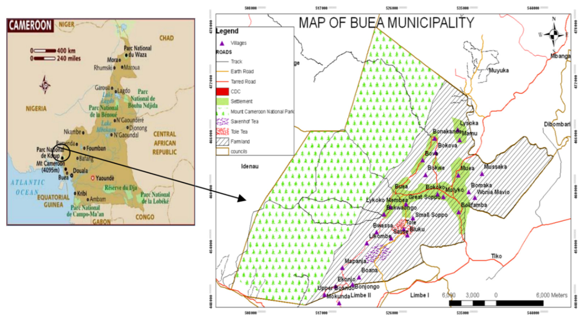
Figure 2.
Map of study corridor (Mile 17 to Governor Roundabout, N8a-8.00km) and Outbound floating car data (Google Earth Pro & Speedometer SS Pro).
Figure 2.
Map of study corridor (Mile 17 to Governor Roundabout, N8a-8.00km) and Outbound floating car data (Google Earth Pro & Speedometer SS Pro).
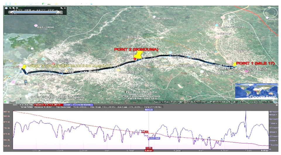
Figure 3.
Images of collection point: (a) P1: Mile 17, regional transit interchange from N8a; (b) P:2 Bonduma, mid segment node; and (c) P3: Governors Roundabout, network study boundary node.
Figure 3.
Images of collection point: (a) P1: Mile 17, regional transit interchange from N8a; (b) P:2 Bonduma, mid segment node; and (c) P3: Governors Roundabout, network study boundary node.
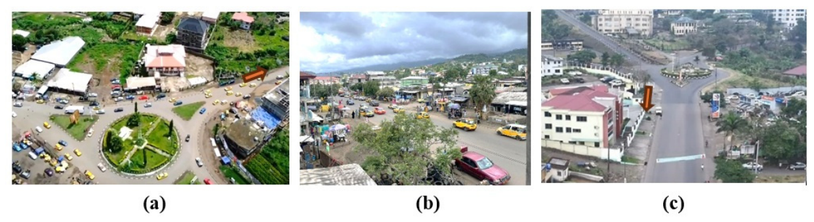
Figure 4.
Inbound flow 15-Minute PCU Volume Profiles per Point, and Peak Periods.
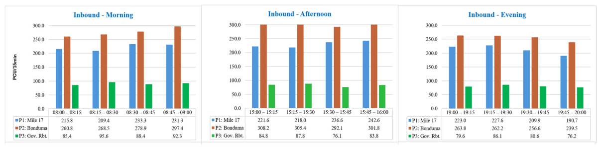
Figure 5.
Outbound flow 15-Minute PCU Volume Profiles per Point, and Peak Periods.
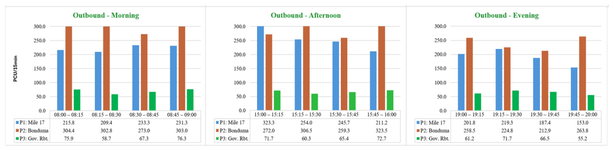
Figure 6.
Directional Flow Asymmetry Index (DFAI) Heatmap, by Measurement Point and Peak Period. Note. Color scale: blue = inbound-dominant (positive DFAI), red = outbound-dominant (negative DFAI), light grey ≈ 0 (symmetric).
Figure 6.
Directional Flow Asymmetry Index (DFAI) Heatmap, by Measurement Point and Peak Period. Note. Color scale: blue = inbound-dominant (positive DFAI), red = outbound-dominant (negative DFAI), light grey ≈ 0 (symmetric).
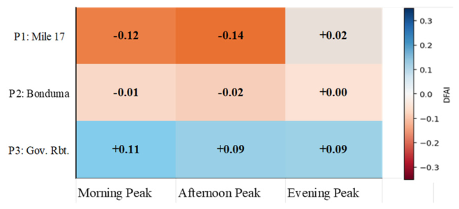
Figure 7.
NEI and CVDR — All Directions and Peak Periods.
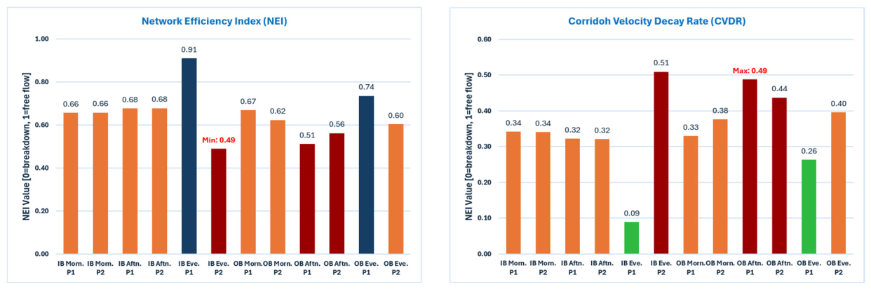
Figure 8.
ITDF — All Directions and Peak Periods.
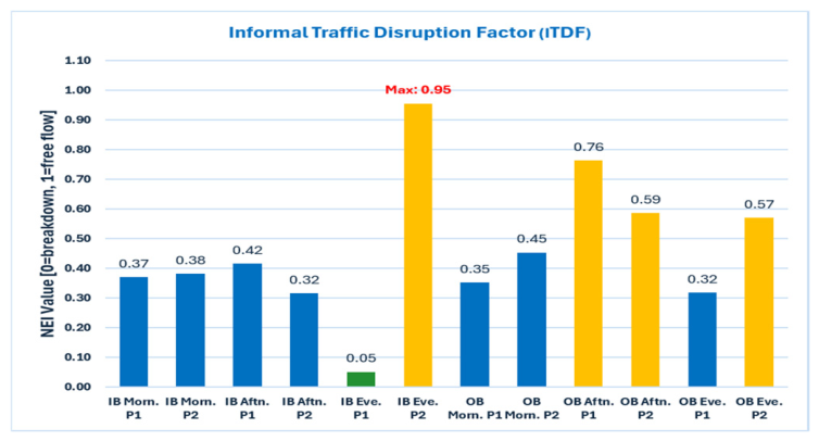
Table 2.
Measurement Point Characteristics.
| Pt. | Name | Dominant Mode | Role in Network |
| P1 | Mile 17 | Mixed traffic (all modes) | Regional transit interchange; primary intercity terminus (gateway node) |
| P2 | Bonduma | Mixed traffic (all modes) | Mid-segment node; highest demand concentration point |
| P3 | Governor’s Roundabout | Mixed traffic (all modes) | Network boundary node; eastern terminus of study corridor |
Table 3.
Inbound (Eastbound) Traffic Flow Summary.
| Point | Period | Vol. (PCU/h) | CV | PHF | Vp (EPCU/h) | v/c | LOS | uobs (km/h) | NEI |
|---|---|---|---|---|---|---|---|---|---|
| Mile 17 (P1) | Morning | 889.8 | 0.11 | 0.95 | 933.1 | 0.77 | C | 21.56 | 0.66 |
| Bonduma (P2) | Morning | 1,105.7 | 0.08 | 0.93 | 1,189.7 | 0.98 | E | 21.60 | 0.66 |
| Gov. Rbt. (P3) | Morning | 361.7 | 0.08 | 0.95 | 382.3 | 0.31 | A | — | — |
| Mile 17 (P1) | Afternoon | 918.8 | 0.08 | 0.95 | 970.6 | 0.80 | D | 22.22 | 0.68 |
| Bonduma (P2) | Afternoon | 1,207.4 | 0.09 | 0.98 | 1,232.7 | 1.01 | F | 22.26 | 0.68 |
| Gov. Rbt. (P3) | Afternoon | 332.4 | 0.18 | 0.95 | 351.3 | 0.29 | A | — | — |
| Mile 17 (P1) | Evening | 851.2 | 0.08 | 0.93 | 910.6 | 0.75 | C | 29.86 | 0.91 |
| Bonduma (P2) | Evening | 1,022.1 | 0.06 | 0.97 | 1,055.3 | 0.87 | D | 16.08 | 0.49 |
| Gov. Rbt. (P3) | Evening | 322.4 | 0.14 | 0.94 | 344.3 | 0.28 | A | — | — |
Note. Over-capacity condition (v/c ≥ 1.00 = LOS F) and evening Bonduma NEI = 0.49 at v/c = 0.87 indicates disproportionate informal-mode speed degradation.
Table 5.
Directional Flow Asymmetry — Inbound vs. Outbound EPCU/h and DFAI.
| Point | Period | IB v (EPCU/h) | OB v (EPCU/h) | DFAI | Dir. Split % | Dominant Direction | LOS IB/OB |
|---|---|---|---|---|---|---|---|
| Mile 17 | Morning | 933.1 | 1,198.6 | −0.12 | 43.8 | Outbound | C / E |
| Bonduma | Morning | 1,189.7 | 1,217.7 | −0.01 | 49.4 | Near symmetric | E / E |
| Gov. Rbt. | Morning | 382.3 | 303.7 | +0.11 | 55.7 | Mildly inbound | A / A |
| Mile 17 | Afternoon | 970.6 | 1,293.1 | −0.14 | 42.9 | Outbound | D / F |
| Bonduma | Afternoon | 1,232.7 | 1,294.0 | −0.02 | 48.8 | Near symmetric | F / F |
| Gov. Rbt. | Afternoon | 351.3 | 290.7 | +0.09 | 54.7 | Mildly inbound | A / A |
| Mile 17 | Evening | 910.6 | 877.3 | +0.02 | 50.9 | Near symmetric | C / C |
| Bonduma | Evening | 1,055.3 | 1,055.3 | 0.00 | 50.0 | Perfectly symmetric | D / D |
| Gov. Rbt. | Evening | 344.3 | 286.7 | +0.09 | 54.6 | Mildly inbound | A / A |
Table 6.
Velocity Decay and Network Efficiency Metrics by Direction and Peak Period.
| Point | Period | Vp (EPCU/h) | uobs (km/h) | uf (km/h) | NEI | CVDR | MTTR | BPR | ITDF | v/c | LOS |
|---|---|---|---|---|---|---|---|---|---|---|---|
| Mile 17 | Morning (IB) | 933.1 | 21.56 | 32.79 | 0.66 | 0.34 | 1.52 | 1.15 | 0.37 | 0.77 | D |
| Bonduma | Morning (IB) | 1,189.7 | 21.60 | 32.79 | 0.66 | 0.34 | 1.52 | 1.14 | 0.38 | 0.98 | E |
| Mile 17 | Afternoon (IB) | 970.6 | 22.22 | 32.79 | 0.68 | 0.32 | 1.48 | 1.06 | 0.42 | 0.80 | D |
| Bonduma | Afternoon (IB) | 1,232.7 | 22.26 | 32.79 | 0.68 | 0.32 | 1.47 | 1.16 | 0.32 | 1.01 | F |
| Mile 17 | Evening (IB) | 910.6 | 29.86 | 32.79 | 0.91 | 0.09 | 1.10 | 1.05 | 0.05 | 0.75 | D |
| Bonduma | Evening (IB) | 1,055.3 | 16.08 | 32.79 | 0.49 | 0.51 | 2.04 | 1.08 | 0.96 | 0.87 | E |
| Mile 17 | Morning (OB) | 1,198.6 | 23.90 | 35.68 | 0.67 | 0.33 | 1.49 | 1.14 | 0.35 | 0.98 | E |
| Bonduma | Morning (OB) | 1,217.7 | 22.26 | 35.68 | 0.62 | 0.38 | 1.60 | 1.15 | 0.45 | 1.00 | E |
| Mile 17 | Afternoon (OB) | 1,293.1 | 18.27 | 35.68 | 0.51 | 0.49 | 1.95 | 1.19 | 0.76 | 1.06 | F |
| Bonduma | Afternoon (OB) | 1,294.0 | 20.08 | 35.68 | 0.56 | 0.44 | 1.78 | 1.19 | 0.59 | 1.06 | F |
| Mile 17 | Evening (OB) | 877.3 | 26.27 | 35.68 | 0.74 | 0.26 | 1.36 | 1.04 | 0.32 | 0.72 | D |
| Bonduma | Evening (OB) | 1,055.3 | 21.56 | 35.68 | 0.60 | 0.40 | 1.65 | 1.08 | 0.57 | 0.87 | E |
Note. uf = free-flow speed from off-peak GPS runs (22:00–05:00): 32.79 km/h eastbound and 35.68 km/h westbound. v/c ≥ 1.00 indicates LOS F over-capacity conditions. Bonduma evening inbound records the highest ITDF in the dataset.
Table 7.
Corridor Performance Summary (All Metrics, All Periods, Both Directions).
| Period | Direction | v/c (P2) | PHF (P2) | NEI (P2) | CVDR (P2) | MTTR (P2) | DFAI (P1) | Peak SCPI | LOS (P1/P2) |
|---|---|---|---|---|---|---|---|---|---|
| Morning | Inbound | 0.98 | 0.93 | 0.66 | 0.34 | 1.48 | −0.22 | 0.55 | C / E |
| Afternoon | Inbound | 1.01 | 0.98 | 0.68 | 0.32 | 1.44 | −0.26 | 0.65 | D / F |
| Evening | Inbound | 0.87 | 0.97 | 0.49 | 0.51 | 1.99 | −0.03 | 0.45 | C / D |
| Morning | Outbound | 1.00 | 0.97 | 0.62 | 0.38 | 1.61 | −0.22 | 0.58 | E / E |
| Afternoon | Outbound | 1.06 | 0.90 | 0.51 | 0.49 | 1.95 | −0.26 | 0.70 | F / F |
| Evening | Outbound | 0.87 | 0.91 | 0.60 | 0.40 | 1.67 | +0.03 | 0.42 | C / D |
Note. Rows with VCR ≥ 1.00 denote over-capacity conditions (LOS F). SCPI values are estimated from the proportion of corridor length operating at VCR ≥ 0.81.
Disclaimer/Publisher’s Note: The statements, opinions and data contained in all publications are solely those of the individual author(s) and contributor(s) and not of MDPI and/or the editor(s). MDPI and/or the editor(s) disclaim responsibility for any injury to people or property resulting from any ideas, methods, instructions or products referred to in the content. |
© 2026 by the authors. Licensee MDPI, Basel, Switzerland. This article is an open access article distributed under the terms and conditions of the Creative Commons Attribution (CC BY) license (http://creativecommons.org/licenses/by/4.0/).
Copyright: This open access article is published under a Creative Commons CC BY 4.0 license, which permit the free download, distribution, and reuse, provided that the author and preprint are cited in any reuse.


