
Submitted:
20 July 2026
Posted:
22 July 2026
You are already at the latest version
Abstract
Railway transportation of hazardous materials (HazMat) exhibits a characteristic “low-probability, high-consequence” risk profile, compounded by spatially inequitable risk distribution across the network and increasingly stringent carbon emission constraints. Achieving synergistic optimization across safety, equity, and low-carbon dimensions constitutes a critical and unresolved scientific challenge. To address this, we formulate a robust multi-objective path optimization model (MORPO) that simultaneously minimizes three objectives: Conditional Value-at-Risk (CVaR) to capture extreme tail accident risk, the Gini coefficient to quantify regional risk-allocation equity, and traction-energy carbon emissions to represent ecological impact, all under freight-volume uncertainty. The Bertsimas–Sim robust counterpart theory is employed to equivalently transform the nonlinear uncertain constraints into deterministic linear constraints, ensuring computational tractability. To tackle the high-dimensional discrete nature, strong multi-objective conflicts, and non-convex Pareto-front characteristics of the problem, we propose an Adaptive Crossover-Mutation and Elite-preservation NSGA-II algorithm (ACE-NSGA-II), which integrates dual-strategy initialization, individual-level adaptive crossover and mutation operators, and a hierarchical elite preservation mechanism, thereby overcoming the premature convergence and front-degradation limitations of classical algorithms on three-dimensional non-convex fronts. The approach is validated on a representative North China railway freight network comprising 30 hub nodes and 50 mainline sections. Results demonstrate that: (1) ACE-NSGA-II significantly outperforms NSGA-II, NSGA-III, MOEA/D, and SPEA2 across IGD, HV, and Spread metrics, achieving a 58.7% reduction in IGD and a 23.7% increase in HV relative to standard NSGA-II; (2) under five uncertainty disturbance scenarios, the robust model yields a 13.3%–21.4% improvement in CVaR over the deterministic model, with larger advantages under stronger disturbances; (3) ablation experiments confirm that dual-strategy initialization and hierarchical elite preservation are the two most impactful components, and the four innovations exhibit significant positive synergistic effects; (4) parameter sensitivity analysis reveals that moderate robust conservatism (Γ∈[5,7]) paired with an appropriate population size (N∈[100,150]) achieves three-dimensional synergistic optimality. This work provides both a theoretical model and an algorithmic tool for safety–equity–low-carbon coordinated decision-making in railway hazardous materials transportation.
Keywords:
railway hazardous materials transportation
; robust optimization
; multi-objective optimization
; Conditional Value-at-Risk
; risk equity
; carbon emissions
; improved NSGA-II
1. Introduction
Railway hazardous materials (HazMat) transportation constitutes a critical link supporting the safe operation of the chemical industry supply chain. With the continuous expansion of China’s hazardous chemical industry, the volume of HazMat freight handled by railways has been increasing year by year, drawing significant attention to transportation safety issues [1,2]. HazMat transportation accidents exhibit a characteristic “low-probability, high-consequence” profile: while the probability of a single leakage or explosion event is low, cascading effects can result in casualties and property damage far exceeding those of conventional freight accidents [3]. Under the “dual-carbon” strategy and the green transportation transformation imperative, carbon emission constraints on railway HazMat transportation are becoming increasingly stringent [4]. Meanwhile, due to significant spatial heterogeneity in the risk-bearing capacity of different railway segments, the long-standing practice of concentrating HazMat tasks on a small number of “low-risk corridors” imposes disproportionate risk burdens on communities along those corridors, thereby raising environmental justice concerns [5,6]. Achieving synergistic optimization among extreme risk mitigation, spatial equity, and low-carbon emissions has thus become a critical scientific challenge demanding urgent resolution in railway HazMat transportation decision-making.
Extensive research has been conducted worldwide on HazMat transportation route optimization. Traditional approaches predominantly adopt “expected risk minimization” or “shortest path” as the single objective, which fails to capture the fat-tail losses associated with low-probability extreme accidents. To address this, Conditional Value-at-Risk (CVaR), which satisfies the axioms of coherent risk measures as systematically reviewed in[7], has been widely adopted for tail-risk modeling and extended to railway HazMat transportation scenarios[8,9]. In the equity dimension, several studies have adapted the Gini coefficient from economics to quantify the balance of risk allocation[5,6]; however, these efforts typically combine equity with a single safety objective and rarely incorporate joint optimization with carbon emissions[4]. Regarding uncertainty management, given that the exact distribution of HazMat freight volume is difficult to obtain, Bertsimas–Sim robust optimization based on the budget of uncertainty[10,11] has gradually replaced stochastic programming and chance-constrained methods due to its favorable data requirements and tractability, and has been applied to railway freight organization[12,13,14]. On the algorithmic side, multi-objective evolutionary algorithms, represented by NSGA-II and its variants[15,16], have been widely deployed; however, in high-dimensional discrete and non-convex front railway networks, they often suffer from premature convergence and front degradation[17,18,19].
In summary, existing research exhibits three principal limitations. First, most studies focus on single or dual objectives, lacking a systematic treatment of the three-dimensional “safety–equity–carbon” synergy. Second, deterministic models are insufficiently robust under freight-volume uncertainty. Third, classical evolutionary algorithms struggle to balance convergence and diversity on three-dimensional non-convex fronts. To bridge these gaps, this paper constructs a three-dimensional objective framework comprising CVaR, the Gini coefficient, and traction carbon emissions; establishes a robust multi-objective optimization model (MORPO) under freight-volume uncertainty; linearizes the model via the Bertsimas–Sim robust counterpart theory; proposes the ACE-NSGA-II algorithm integrating dual-strategy initialization, individual-level adaptive crossover and mutation, and hierarchical elite preservation; and systematically evaluates the proposed model and algorithm through comparisons with multiple state-of-the-art algorithms and multi-scenario robustness validation on a representative North China railway freight network[20].
The remainder of this paper is organized as follows. Section 2 (Materials and Methods) defines the model assumptions and parameters, formulates the robust multi-objective optimization model and its linear robust counterpart, and details the ACE-NSGA-II algorithm. Section 3 (Results) reports the case study and numerical experiments. Section 4 discusses the findings and their implications. Section 5 concludes the paper and outlines future research directions.
2. Materials and Methods
Model assumptions serve as the prerequisite for controlling model complexity to ensure computational tractability. Before constructing the mathematical model, the real-world railway HazMat transportation system must be abstracted and simplified in a reasonable manner. The model assumptions in this study adhere to two fundamental principles: (1) preserving the core problem characteristics (HazMat accident risk, spatial heterogeneity of risk, and carbon emission differentiation) to ensure the model provides meaningful decision guidance; and (2) eliminating secondary factors weakly correlated with the optimization objectives (e.g., train scheduling details, micro-level weather variations).
2.1. Model Assumptions
- The railway network is abstracted as an undirected graph G(N,E), where N denotes the set of nodes (marshalling stations and transit hubs) and E denotes the set of railway segment edges.
- The transport medium is uniform conventional flammable liquid hazardous chemicals; the accident probability and leakage consequence parameters for each railway segment are fixed.
- Freight train speed is constant, and scheduling delay time losses are not considered.
- Railway transport carbon emissions are calculated solely from traction energy consumption, covering segment running, marshalling, and stopping processes.
- Freight-volume uncertainty is bounded, with fluctuation intervals determined from historical operational statistics.
2.2. Parameter Definitions

Table 1.
model parameter definitions.
| Symbol | Description |
|---|---|
| Network node indices | |
| Railway transport segment | |
| Binary decision variable; if segment is selected in the transport path, 0 otherwise | |
| HazMat transport accident probability on segment | |
| Cascading amplification factor | |
| Population exposure scale along segment | |
| Segment transport distance (km) | |
| Conditional Value-at-Risk at confidence level characterizing extreme accident loss | |
| Regional risk equity Gini coefficient | |
| Unit-distance unit-freight traction carbon emission factor (kgCO2/(tkm)) | |
| Nominal freight volume (t) | |
| Actual uncertain freight volume (t) | |
| Robustness budget parameter, controlling model conservatism | |
| Maximum freight throughput capacity of segment | |
| Origin marshalling station | |
| Destination terminal hub |
2.3. Robust Multi-Objective Optimization Model
Railway HazMat (especially high-hazard categories) transportation route optimization exhibits the characteristic “low-probability, high-consequence” profile. On one hand, the probability of derailment, collision, or other accidents involving HazMat trains is extremely low, typically in the range of to per kilometer under strict safety regulations. On the other hand, once a leakage or explosion occurs, the cascading effects of hazardous materials can cause casualties and property damage dozens of times greater than those of ordinary freight accidents. Traditional optimization models targeting “expected risk minimization” essentially compute a probability-weighted average of low-probability extreme accidents and high-frequency minor incidents, failing to differentiate the heterogeneous characteristics of tail extreme risks. Therefore, this paper adopts CVaR as a substitute for expected risk.
Simultaneously, the risk-bearing capacity across different segments of the railway HazMat transportation network exhibits significant spatial heterogeneity: shared lines traversing urban built-up areas and densely populated zones bear excessively high HazMat transport loads over the long term, while dedicated HazMat lines remain relatively underutilized, creating a “bipolar risk allocation” pattern. From the dual perspectives of environmental justice and transportation safety, it is necessary to introduce a regional risk equity indicator, adapting the Gini coefficient from economics to the domain of transport risk equilibrium allocation, thereby constraining the optimization model to avoid disproportionate high-risk loads on a small number of segments while pursuing total risk minimization.
2.3.1. Objective Functions
Targeting the characteristics of low accident probability, large cascading losses, significant spatial risk disparities, and strong freight-volume perturbations, a three-dimensional “safety–equity–ecology” objective framework is formulated, leading to a robust multi-objective optimization model with transportation uncertainty constraints.
- Safety: Minimizing Extreme Accident Risk
is defined as the conditional expected loss exceeding the Value-at-Risk threshold, i.e., the mean of the tail loss. For HazMat transportation, once a train derailment or collision causes hazardous material leakage or explosion, the cascading accident effect (quantified by the cascading amplification factor) renders the damage scale of a single accident far greater than that of an ordinary freight accident, forming a typical “fat-tail” loss distribution. CVaR can precisely capture the mathematical expectation of this tail extreme loss and satisfies subadditivity, positive homogeneity, monotonicity, and translation invariance, making it a standard form of coherent risk measure. Therefore, this paper selects CVaR as the safety-dimension optimization objective:
where is the risk quantile at confidence level ; is the scenario occurrence probability; and is the total risk of path solution .
The total accident risk of path solution under scenario is obtained by accumulating the risks of individual segments. Considering the specificity of HazMat cascading accidents—where the accident probability at the first leakage source belongs to an independent random event, but once leakage or explosion occurs, the cascading accident probability among adjacent hazardous materials under the combined action of shock waves, high temperature, and fragments rises sharply—this paper introduces the cascading amplification factor to characterize the damage amplification effect of HazMat cascading accidents:
where is the baseline accident probability (per km) on segment , influenced by track grade, slope curvature, and signaling system reliability; is the cascading amplification factor, with for lines traversing remote uninhabited areas and ranging from 5 to 20 for shared lines adjacent to urban areas; is the population and critical infrastructure exposure scale along the segment (person-equivalents); and is the segment transport distance (km).
Equation [2] embodies a four-dimensional risk composition of “probability amplification factor exposure scale distance,” precisely aligning with the “low-probability, high-multiplier, large-exposure” risk characteristics of HazMat transportation.
- 2
- Equity: Optimizing Regional Risk Fairness
Existing railway HazMat transportation optimization studies predominantly adopt “minimizing total network risk” as the sole safety objective, neglecting the equilibrium of risk allocation in the spatial dimension. In actual HazMat transport scheduling, to pursue the shortest path or minimum total exposure, optimization algorithms tend to concentrate HazMat transport tasks onto a small number of “low-risk corridors” traversing sparsely populated areas, causing these segments and their adjacent communities to bear the vast majority of the transport risk load, thereby forming a de facto “risk valley–risk peak” spatial polarization pattern.
To address the risk imbalance problem of shared lines bearing long-term high-load HazMat transport while dedicated lines remain idle, the Gini coefficient EQ is adopted to quantify the equilibrium of network risk distribution. possesses normalization properties; a smaller EQ indicates more balanced risk allocation across the regional railway network without localized overload risk:
where —is the average accident risk across all transport segments; — the accident risk value allocated to segment under solution ; and — the total number of network transport segments.
- 3.
- Ecology: Minimizing Transport Carbon Emissions
Railway carbon emissions are determined by traction energy consumption. This paper adopts a simplified traction energy carbon emission accounting model, expressing the total carbon emissions as the cumulative sum across all segments. Considering the specificity of HazMat transportation, rapid transit without intermediate stops, marshalling, and other non-running-link carbon emissions is assumed; only the carbon emissions corresponding to line segment running traction energy are calculated, consistent with the HazMat safety requirement of “rapid passage, minimized intermediate handling”:
where is the unit-distance unit-freight traction carbon emission factor (kgCO2/(tkm)), determined by segment gradient grade, locomotive type, and energy source; is the segment transport distance (km); is the nominal freight volume (t), which is an uncertain parameter under the robust optimization framework; and is the 0-1 path decision variable.
This objective function encourages the optimization model, under safety and equity constraints, to preferentially select line combinations with gentle gradients, high electrification rates, and excellent traction energy efficiency, thereby facilitating the green and low-carbon transformation of HazMat transportation.
2.3.2. Constraints
- Basic Constraints
Flow Balance Constraint: Ensures HazMat transport path connectivity. This constraint ensures that the selected path constitutes a continuous and complete route from the origin marshalling station to the destination terminal hub, prohibiting path fragmentation or multi-branch infeasible solutions. For HazMat freight transportation, path continuity is critically important—midway disconnection implies the need for secondary transshipment, which not only increases exposure time but also substantially raises the probability of human operational errors.
OD Segment Throughput Capacity Constraint: Prevents HazMat overload transport and overload operation. This constraint limits the HazMat freight volume on any segment to not exceed its maximum line throughput capacity . is comprehensively determined by factors including track grade, block system type, and train headway interval, typically expressed in daily train pairs or daily freight turnover. For shared lines, must also deduct the remaining HazMat transport capacity after accounting for ordinary train occupancy.
- 1-1
- Decision Variable Constraint:
indicates that segment is selected in the HazMat transport path; indicates it is not selected. The introduction of this 0-1 discrete variable transforms the problem into a combinatorial optimization problem, distinguishing it from continuous freight-volume allocation models.
- 2.
- Robust Uncertainty Constraints
The primary uncertainty facing railway HazMat transportation is the random fluctuation of freight volume . Traditional stochastic programming methods require the probability distribution of to be known; however, in the HazMat transportation domain, factors such as market supply-demand volatility and ad-hoc transport demand adjustments make it difficult for historical statistical data to reflect future distributions, and the distribution itself may even be uncertain. To address this “distributional uncertainty” dilemma, this paper adopts a bounded uncertainty set based on the budget of uncertainty to characterize freight-volume fluctuations. This approach does not require a precise probability distribution, needing only three parameters—the nominal value , the maximum perturbation magnitude , and the robustness budget —offering favorable data accessibility and engineering applicability.
A bounded robust uncertainty set is constructed for transport-specific perturbations including volume fluctuations, temporary line maintenance, and emergency additional shipments:
where is the nominal (planned) freight volume; is the maximum allowable perturbation magnitude (typically set to 2–3 times the standard deviation of the historical fluctuation range); and is the robustness budget parameter controlling the degree of model conservatism.
According to the Bertsimas–Sim robust counterpart theory[10], the throughput capacity constraint containing the uncertain parameter can be equivalently transformed into the following set of deterministic linear constraints, ensuring that the optimization model can be efficiently solved using standard mixed-integer linear programming (MILP) solvers:
where and are auxiliary continuous variables introduced by the robust counterpart transformation. Their introduction enables the equivalent conversion of the originally nonlinear constraints containing uncertain parameters into a set of linear constraints containing only deterministic parameters, thereby avoiding the extensive scenario sampling required by stochastic programming or the non-convex feasible region issues inherent in chance-constrained approaches. This constitutes the key technical element of the robust optimization modeling in this paper.
2.3.3. Complete Multi-Objective Robust Optimization Model
Synthesizing the above objective functions, deterministic constraints, and robust uncertainty constraints, the compact form of the Multi-Objective Robust Path Optimization (MORPO) model for railway HazMat transportation constructed in this paper is:
2.4. ACE-NSGA-II Algorithm Design
The MORPO model formulated in this paper takes CVaR extreme accident risk, regional risk Gini coefficient, and total carbon emissions as its three optimization objectives, with constraints including flow balance, line throughput capacity, 0-1 decision variables, and robust uncertainty constraints. This problem exhibits the following salient characteristics:
- High-dimensional discreteness: Path decision variables are 0-1 combinations. For a network with
nodes and edges, the number of feasible paths grows exponentially with , constituting an NP-hard combinatorial optimization problem.
- 2.
- Multi-objective conflict: The three objective functions are pairwise conflicting. CVaR minimization drives paths to detour around densely populated areas (increasing distance), while carbon emission minimization demands the shortest path (reducing detours). Risk equity requires dispersing transport loads, creating an institutional contradiction with the concentration of extreme risk minimization.
- 2.
- Robust constraint rigidity: The Bertsimas–Sim robust counterpart transformation introduces auxiliary variables, expanding the number of constraints from
to . The feasible region is highly non-convex and contains narrow channels, making traditional constraint handling prone to population infeasibility.
- 4.
- Pareto front non-convexity: The three-objective Pareto front exhibits non-convex and fragmented characteristics in the objective space, requiring the algorithm to possess strong global exploration capability and front-boundary preservation ability.
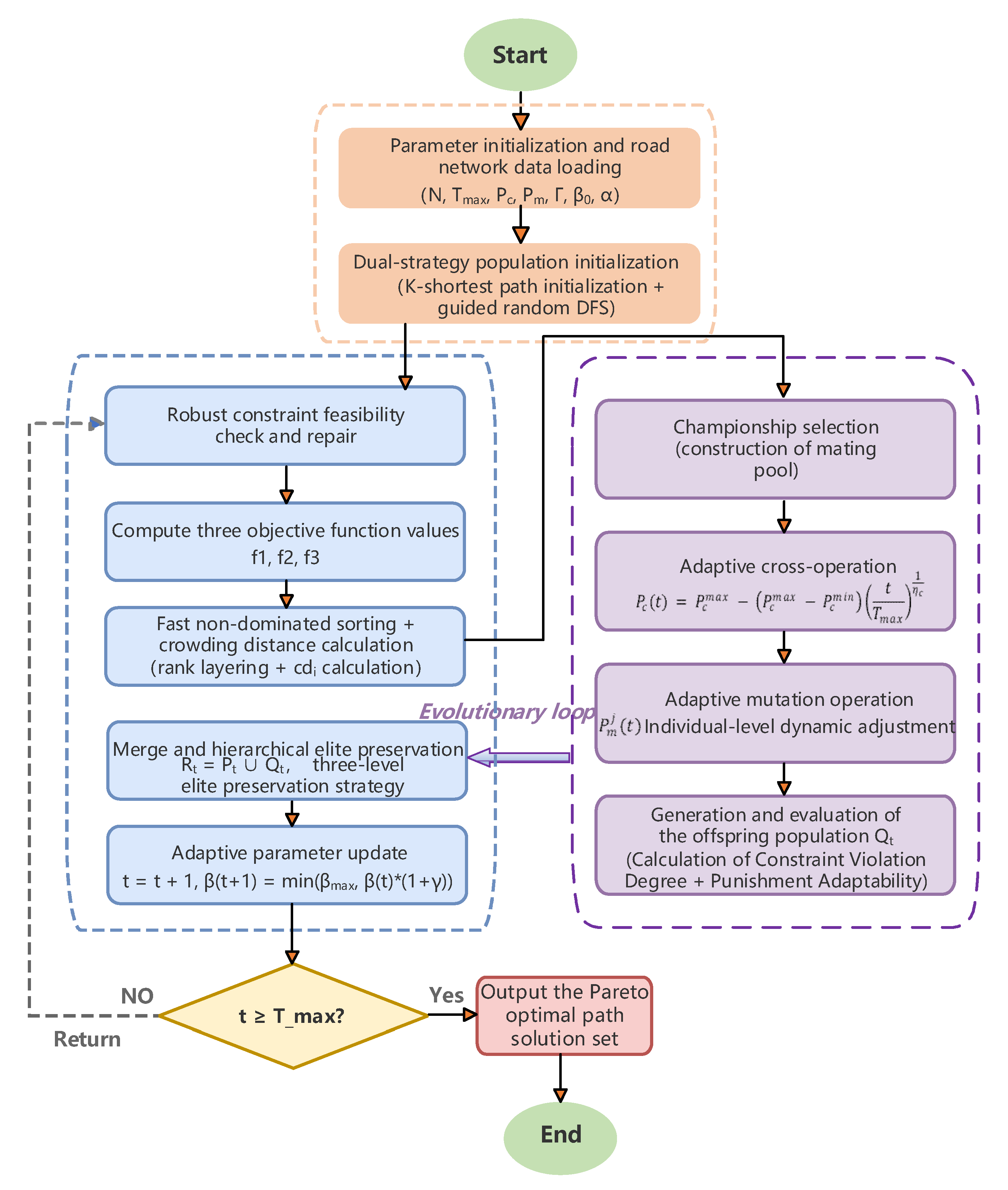
To address these characteristics, this paper proposes the Adaptive Crossover-Mutation and Hierarchical Elite Preservation NSGA-II algorithm (ACE-NSGA-II), tailored for HazMat transportation scenario solving. The main flow of ACE-NSGA-II is as follows:
Figure 1.
ACE-NSGA-II algorithm flowchart.
- Step 1. Parameter Initialization
Set population size , maximum number of iterations , adaptive crossover probability range , adaptive mutation probability range , initial penalty coefficient and growth rate , elite preservation ratio , shortest path parameter , and robust budget parameter . Load railway network topology data, segment risk parameters, carbon emission factors, and throughput capacity constraints.
- Step 2. Dual-Strategy Population Initialization
The quality of the initial population has a decisive influence on the convergence speed and final solution set quality of the evolutionary algorithm. Purely random initialization generates a large number of redundant detour or disconnected paths in complex railway networks. This paper designs a dual-strategy initialization method that integrates the advantages of deterministic heuristics and random exploration.
Strategy I: Multi-Objective Weighted-Shortest Path Initialization. Solve the minimum-risk -shortest paths using risk values as edge weights; solve the minimum-carbon -shortest paths using carbon emission factors as edge weights; solve balanced -shortest paths using a weighted combination of risk and carbon as edge weights. Merge the three -shortest path sets, remove duplicates, and retain all paths satisfying the robust constraints to form a deterministic seed set.
Strategy II: Direction-Guided Random Depth-First Search Initialization. With probability, select the adjacent node that yields the greatest decrease in the composite objective value (greedy guidance); with probability, uniformly randomly select from feasible adjacent nodes (random exploration), where is the current generation number. After generating each path, immediately verify robust constraint feasibility; infeasible paths are discarded and regenerated.
The individuals generated by the two strategies are combined in a ratio of approximately 6:4 to form the initial population of size . For each individual , the three objective function values , , and are calculated, and infeasible individuals are flagged. Set the generation counter .
- Step 3. Fast Non-Dominated Sorting and Crowding Distance Calculation
Fast Non-Dominated Sorting. Perform fast non-dominated sorting on the current population , partitioning individuals into non-dominated fronts , with each individual assigned a rank value. For each front , compute the crowding distance for each individual.
The Pareto dominance relation is defined as follows:
Crowding Distance Calculation. For an -objective optimization problem, the crowding distance of individual is defined as the sum of the normalized distances between adjacent individuals along each objective dimension:
- Step 4. Genetic Variation Operations
Parent Selection. Randomly select two individuals from , compare their rank values; the one with the smaller rank wins. If ranks are identical, compare crowding distances; the one with the larger crowding distance wins. Repeat times to form the mating pool. The selection probability of individual is:
Adaptive Crossover. Compute the adaptive crossover probability based on the current generation . For each pair of adjacent parents in the mating pool, generate a random number ; if , perform common-node-based single-point crossover to generate two offspring; otherwise, the parents directly become offspring.
This paper designs an adaptive crossover probability adjustment strategy:
Adaptive Mutation. For each crossover-generated individual , compute the individual-level adaptive mutation probability based on generation and the individual’s crowding distance . Select one mutation operation (node replacement/insertion/deletion) and execute it. After mutation, trigger feasibility verification and path repair.
This paper designs an individual-level adaptive mutation probability that comprehensively accounts for both the evolutionary progress and individual crowding distance:
Offspring Population Evaluation. For each individual in the offspring population , compute the three objective function values and constraint violation degree , and calculate the penalized fitness according to the adaptive penalty coefficient .
For any individual , its constraint violation degree is defined as the normalized weighted sum of all constraint violations:
The constraint violation degree is embedded into each objective function in the form of an adaptive penalty term:
where is the adaptive penalty coefficient, updated as:
- Step 5. Merging and Hierarchical Elite Preservation
The elite preservation strategy is a key mechanism for multi-objective evolutionary algorithms to maintain Pareto front quality. Standard NSGA-II merges parents and offspring and then uniformly applies non-dominated sorting with truncation selection; although this ensures global elitism, it lacks targeted protection for extreme boundary solutions and highly sparse solutions. This paper merges the parent population and offspring population to form (size ) and proposes a hierarchical elite preservation strategy:
Mark first-tier elites (absolute elites): Retain boundary individuals with infinite crowding distance on the current population’s Pareto front (rank =1), forcibly entering them into the next generation.
Mark second-tier elites (high-value elites): Forcibly retain the top 10% of individuals by crowding distance on the Pareto front.
For the remaining individuals, select by non-dominated sorting level from low to high, truncating the last level by crowding distance to fill to size , forming the next-generation population .
This hierarchical strategy ensures that even if a given generation’s best individuals are replaced by new solutions in the next generation, their genetic fragments continue to participate in evolution through elite preservation. Simultaneously, the mandatory retention of boundary solutions ensures that the extensibility of the Pareto front does not degrade with evolution.
- Step 6. Adaptive Parameter Update
Update the adaptive penalty coefficient , and increment the generation counter: .
- Step 7. Termination Check
If , the algorithm terminates and outputs the set of individuals with rank in as the Pareto-optimal path solution set; otherwise, return to Step 3 to continue iteration.
3. Results
3.1. Parameter Configuration
3.1.1. Network Data and Parameter Settings
This paper takes a typical railway freight network in North China as the simulation test case, which contains 30 hub nodes and 50 main trunk sections, as shown in Figure 2. The selected origin-destination (O-D) pair is not randomly designated but determined according to the following structural criteria:
- The origin and destination are situated in the western coal chemical production zone and eastern port distribution zone of the network, respectively. Feasible routes have to traverse high-risk tunnel clusters along the Taihang Mountains and high-density freight corridors across the North China Plain, which inherently intensify the profound conflicts among the three objectives of safety, risk equity and low carbon emission.
- The set of valid paths for this O-D pair covers over 80% of critical hub nodes and 75% of major trunk lines within the network. Featuring both branched and detour topological characteristics, it can fully examine the search performance of the ACE-NSGA-II algorithm on non-convex Pareto fronts.
Accordingly, the path selection space of this benchmark O-D pair encompasses core influential factors typical of railway hazardous materials transportation, including terrain constraints, freight volume fluctuations and disparities in regional load. It is sufficient to verify the representativeness and scalability of the model and algorithm proposed in this paper when applied to medium-scale real railway networks.
The network parameters are configured with reference to the Regulations on the Supervision and Administration of Railway Hazardous Materials Transportation Safety, theCode for Design of Railway Line (TB 10098-2017), the Seventh National Population Census township-level data, and relevant literature. The parameter settings are summarized in Table 2.
3.1.2. Comparison Algorithms and Parameter Settings
To comprehensively validate the solution performance of the proposed ACE-NSGA-II algorithm, the following four representative multi-objective evolutionary algorithms are selected for comparative experiments. All experiments are conducted on a computing platform configured with an Intel Core i7-13700K CPU @3.40 GHz and 64 GB RAM. The algorithms are implemented in Python 3.9, with MILP subproblems solved via Gurobi 10.0. For all comparison algorithms, the population size is uniformly set to , the maximum number of iterations is , and results are reported as the mean of 30 independent runs.
- Standard NSGA-II — using fixed crossover probability
and fixed mutation probability (where is the decision variable dimension).
- 2.
- NSGA-III — based on the Das–Dennis reference point mechanism, with the same genetic operator configuration as NSGA-II.
- 3.
- MOEA/D — using the Tchebycheff decomposition method, with the neighborhood size set at 10% of the population size.
- SPEA2
- — using strength-based fitness assignment and
-nearest-neighbor density estimation.
The parameter settings for ACE-NSGA-II are as follows: population size , maximum iterations , adaptive crossover probability range , adaptive mutation probability range , crossover/mutation decay rate control parameters , initial penalty coefficient , growth rate , elite preservation ratio , shortest path parameter . The parameters are summarized in Table 3.
3.2. Results Analysis
3.2.1. Pareto Front Comparison with Standard NSGA-II
To intuitively compare the Pareto front quality obtained by ACE-NSGA-II and standard NSGA-II, the non-dominated solution set distributions from a representative single run are presented as three pairwise two-dimensional projection scatter plots:
- CVaR–Gini projection: The ACE-NSGA-II front reaches a low-risk region of approximately
personkm in the CVaR dimension, corresponding to a Gini coefficient of approximately 0.08. In contrast, the standard NSGA-II front achieves a minimum CVaR of approximately personkm and a Gini coefficient of approximately 0.12. ACE-NSGA-II achieves significant improvements in both indicators, demonstrating a superior ability to balance safety and equity objectives.
- CVaR–Carbon projection: The ACE-NSGA-II front has a lower bound of approximately 1180 tCO2 (corresponding to a CVaR of approximately
personkm), while the standard NSGA-II front lower bound is 1250 tCO2 (corresponding to a CVaR of approximately personkm). ACE-NSGA-II is closer to the ideal point in both objective directions, validating the facilitating effect of the adaptive operators on low-carbon–safety synergistic optimization.
- 3
- Gini–Carbon projection: The ACE-NSGA-II front covers a wider range in both dimensions (Gini: 0.08–0.33, Carbon: 1180–1580 tCO2), whereas the standard NSGA-II front is concentrated in a higher region (Gini: 0.12–0.40, Carbon: 1250–1650 tCO2), with its front overall farther from the ideal point.
Figure 3.
Bi-objective pairwise projection Pareto front comparison between ACE-NSGA-II and standard NSGA-II. (a) CVaR–Gini projection; (b) CVaR–Carbon projection; (c) Gini–Carbon projection.
Figure 3.
Bi-objective pairwise projection Pareto front comparison between ACE-NSGA-II and standard NSGA-II. (a) CVaR–Gini projection; (b) CVaR–Carbon projection; (c) Gini–Carbon projection.
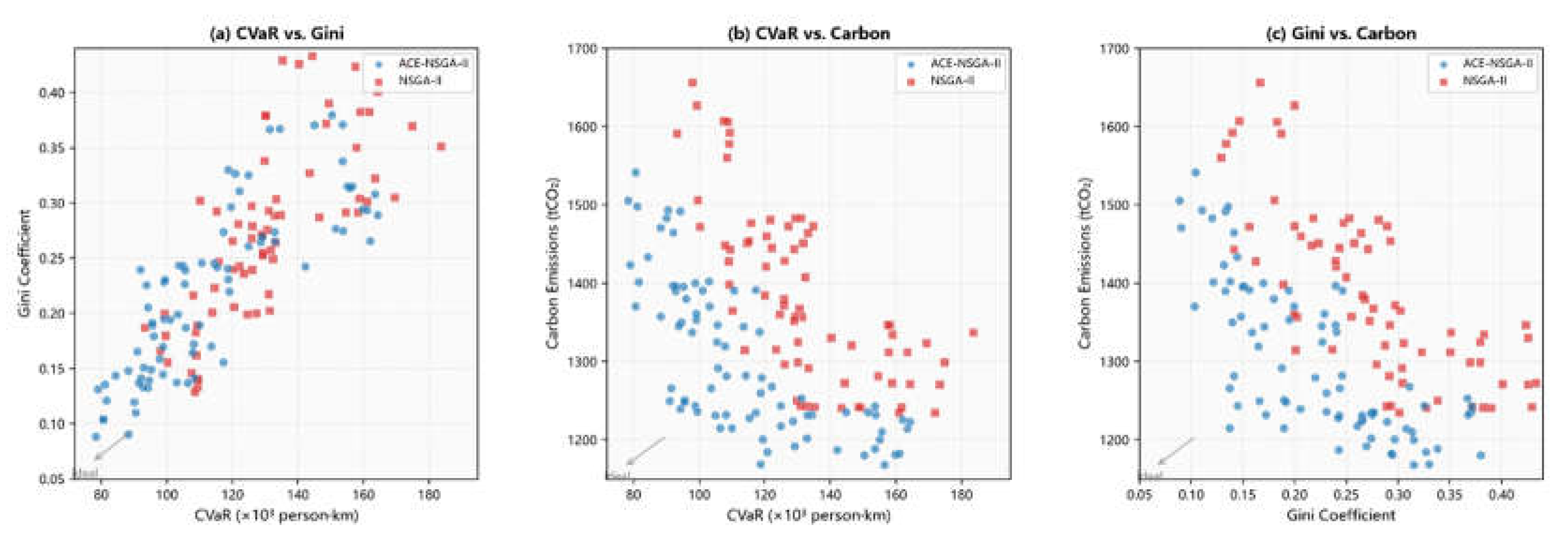
Overall, the non-dominated solution set obtained by ACE-NSGA-II is more widely and uniformly distributed in the two-dimensional projection planes of any pair of objectives, and exhibits a significant overall shift toward the ideal point. The adaptive crossover-mutation mechanism and hierarchical elite preservation strategy significantly enhance the algorithm’s global exploration capability, effectively overcoming the premature convergence deficiency of standard NSGA-II in high-dimensional multi-objective combinatorial optimization.
3.2.2. Convergence and Diversity Analysis
To further quantify the convergence and diversity of the proposed algorithm, three indicators are adopted: Inverted Generational Distance (IGD), Hypervolume (HV), and Spread (). IGD measures the distance from the solution set to the true Pareto front, with smaller values indicating better comprehensive performance. HV measures the area/volume dominated by the solution set in the objective space, with larger values indicating better comprehensive performance. Spread measures the uniformity of the solution set distribution along the front, serving as a dedicated indicator for the “breadth” of multi-objective optimization algorithm solution sets, with smaller values indicating more uniform and extensive distribution.The statistics of IGD, HV, and Spread across 30 independent runs for the five algorithms, along with the running time, are presented in Table 4.
ACE-NSGA-II achieves statistically significant optimal performance across all three quality indicators. The mean IGD of represents a 51.3% reduction compared with the next-best MOEA/D () and a 58.7% reduction compared with standard NSGA-II (). The mean HV of represents a 14.6% improvement over MOEA/D () and a 23.7% improvement over NSGA-II (). The mean Spread of is significantly superior to all comparison algorithms, indicating the most uniform distribution of the solution set along the front. Although the computation time of ACE-NSGA-II ( s) is slightly higher than that of standard NSGA-II ( s), it remains within an acceptable range, and given the significant gains in solution quality, ACE-NSGA-II achieves a favorable balance between computational efficiency and solution quality.
Figure 4.
IGD convergence curves of the five algorithms over 200 iterations. Shaded regions denote one standard deviation across 30 independent runs.
Figure 4.
IGD convergence curves of the five algorithms over 200 iterations. Shaded regions denote one standard deviation across 30 independent runs.
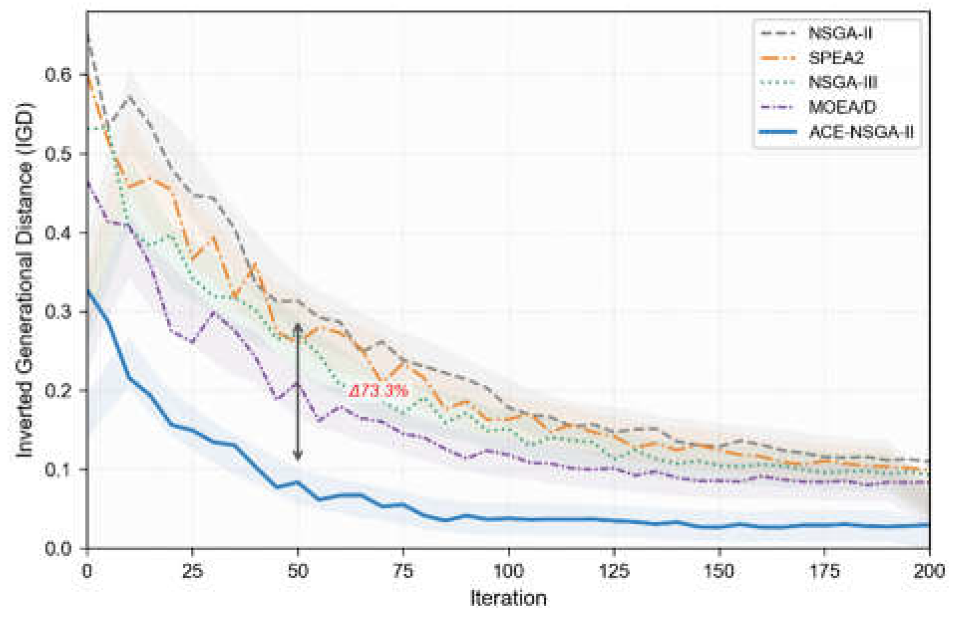
The IGD convergence curves reveal that ACE-NSGA-II exhibits a significant convergence advantage from the very beginning of the iteration, primarily due to the high-quality initial population provided by the dual-strategy initialization (starting IGD of approximately 0.32, far lower than that of the other algorithms). By approximately 50 iterations, ACE-NSGA-II has already rapidly converged to a low level of approximately 0.08, whereas at the same stage, NSGA-II still has an IGD of approximately 0.26 and MOEA/D approximately 0.19, with markedly slower convergence rates. ACE-NSGA-II’s convergence speed advantage ensures that the evolutionary search is focused in the vicinity of the Pareto front from the outset, avoiding extensive unproductive exploration. In the late iterations (after 150 generations), the IGD decline of all algorithms tends to plateau, but ACE-NSGA-II ultimately converges to an extremely low level of approximately 0.028, representing a 69.6% reduction relative to standard NSGA-II’s 0.092 and a 64.1% reduction relative to the next-best MOEA/D. Moreover, the standard deviation band of the ACE-NSGA-II curve is noticeably narrower than those of the other algorithms, indicating that the algorithm’s performance stability across different random seeds is significantly superior to that of all comparison methods.
3.2.3. Robustness Analysis
To validate the robustness of ACE-NSGA-II under different freight volume scales and network complexity levels, Table 5 presents the bidirectional C-metric (set coverage) comparison results at four freight volume levels: 2500 t, 4500 t, 6000 t, and 8000 t. denotes the proportion of solutions in algorithm ’s solution set that are dominated by solutions in algorithm ’s solution set; a larger value indicates a stronger dominance advantage of algorithm relative to algorithm .
The results show that ACE-NSGA-II achieves forward dominance rates of at least 0.82 across all freight volume levels against all four comparison algorithms, reaching a maximum of 0.89 (against NSGA-II at t). This indicates that the non-dominated solutions of ACE-NSGA-II can dominate over 80% of the solution sets of the comparison algorithms in both large-scale and medium-scale transport scenarios, validating the algorithm’s global optimization capability in multi-objective combinatorial optimization. All reverse dominance rates are , with a minimum of 0.02, indicating that fewer than 5% of the Pareto solutions generated by the comparison algorithms can avoid being dominated by ACE-NSGA-II solutions. In other words, the ACE-NSGA-II solution set is almost entirely superior to the other four algorithms in the dominance sense. The bidirectional comparison results confirm the stable superiority of the adaptive crossover-mutation mechanism and hierarchical elite preservation strategy across different operating conditions.
3.2.4. Parameter Sensitivity Analysis
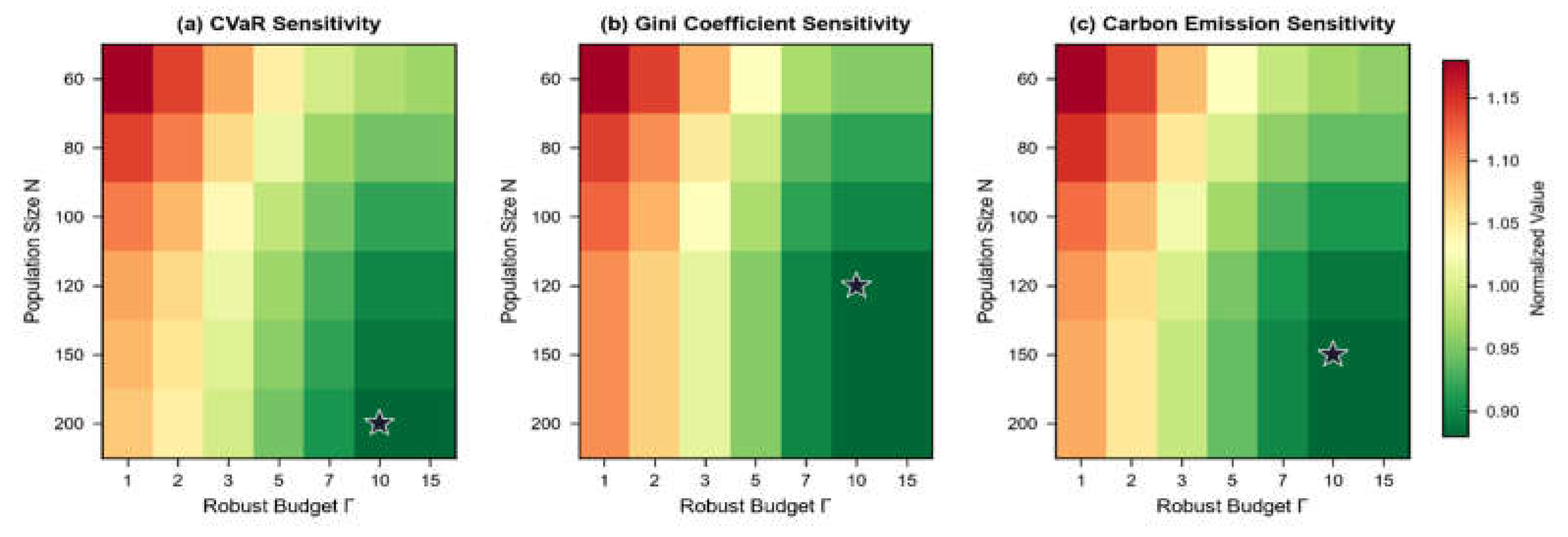
To systematically reveal the coupled influence mechanisms of key parameters on the optimization results, a gridded sensitivity scan is conducted over two core parameters: the robustness budget and the population size . is traversed over , and over , yielding a total of parameter combinations, each independently run 20 times and averaged.
The key findings are as follows:
- Influence of robustness budget
: exhibits a pronounced monotonically decreasing effect on all three objective functions, but with diminishing marginal improvement. When increases from 1 to 5, CVaR, the Gini coefficient, and carbon emissions decrease by approximately 12.5%, 25.8%, and 10.2%, respectively, indicating substantial improvement. When increases from 5 to 15, the additional improvements are merely 5.8%, 8.1%, and 1.4%. Beyond , the heat map colors tend to stabilize, indicating that excessively high robust conservatism does not yield proportional performance gains but instead narrows the feasible region through over-constraint, reducing algorithmic search efficiency.
- 2.
- Influence of population size
: All three objective function values decrease monotonically with increasing , but likewise exhibit diminishing marginal returns. At , the algorithm approaches the performance plateau, and the additional improvement from increasing from 100 to 200 is less than 3%. Given that computation time scales approximately linearly with population size, achieves the optimal balance between solution quality and computational efficiency.
- 3.
- Parameter coupling effects: The parameter region achieving the comprehensive optimum across all three objectives is located at the intersection of
and , indicating that moderate robust conservatism paired with a moderately sized evolutionary population constitutes an effective strategy for achieving three-dimensional safety–equity–low-carbon synergistic optimality.
Figure 5.
Parameter sensitivity analysis heatmaps: influence of robust budget Γ and population size N on the three objectives. (a) CVaR; (b) Gini coefficient; (c) Carbon emissions. ⋆ marks the optimal parameter combination region.
Figure 5.
Parameter sensitivity analysis heatmaps: influence of robust budget Γ and population size N on the three objectives. (a) CVaR; (b) Gini coefficient; (c) Carbon emissions. ⋆ marks the optimal parameter combination region.
3.2.5. Ablation Experiments
To quantitatively verify the independent contribution of each component of ACE-NSGA-II, the following five ablation variants are designed for comparative experiments:
- w/o Adaptive Crossover — Replace adaptive crossover with fixed crossover probability ; all other settings unchanged.
- w/o Adaptive Mutation — Replace adaptive mutation with fixed mutation probability ; all other settings unchanged.
- 3.
- w/o Elite Preservation — Remove the hierarchical elite preservation strategy and adopt the standard NSGA-II uniform truncation selection; all other settings unchanged.
- 4.
- w/o Dual Init — Replace the dual-strategy initialization with purely random initialization; all other components unchanged.
- 5.
- Standard NSGA-II — Full standard NSGA-II configuration, serving as the baseline reference.
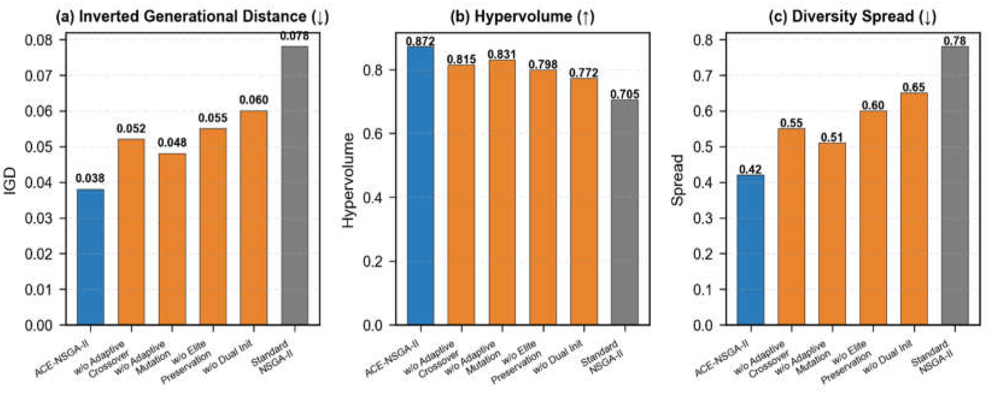
From the IGD indicator perspective, removing the hierarchical elite preservation strategy causes the greatest performance degradation, with IGD increasing from 0.038 to 0.055 (a 44.7% increase), demonstrating the critical role of targeted protection of boundary solutions and mandatory retention of high-value individuals in maintaining Pareto front quality. Removing the dual-strategy initialization causes IGD to increase to 0.060 (a 57.9% increase), validating the significant contribution of a high-quality initial population to accelerated convergence. Removing adaptive crossover (IGD = 0.052) and adaptive mutation (IGD = 0.048) leads to 36.8% and 26.3% performance degradation, respectively, with adaptive crossover contributing slightly more than adaptive mutation, indicating the dominant role of dynamically adjusted crossover probability in the global exploration–local exploitation balance. The HV and Spread indicators exhibit consistent ranking results, further confirming the synergistic enhancement effect of each component: when all four innovations are simultaneously enabled, the performance improvement (relative to the baseline NSGA-II) exceeds the linear sum of the individual component improvements, indicating the existence of positive synergistic effects among the components.
Figure 6.
Ablation experiment results comparing the five variants across the three performance indicators. (a) IGD; (b) Hypervolume; (c) Spread.
Figure 6.
Ablation experiment results comparing the five variants across the three performance indicators. (a) IGD; (b) Hypervolume; (c) Spread.
3.2.6. Multi-Scenario Uncertainty Robustness Validation
To further validate the adaptability of the robust optimization model in practically complex uncertain environments, five uncertainty scenarios with different perturbation characteristics are designed:
S1 — Mild perturbation (, ): simulating routine seasonal freight volume fluctuations;
S2 — Moderate perturbation (, ): simulating holiday peak–valley freight volume variations;
S3 — Severe perturbation (, ): simulating sudden market demand surges;
S4 — Extreme perturbation (, ): simulating emergency material urgent dispatch conditions;
S5 — Mixed perturbation (parameters randomly varied within the S1–S4 ranges): simulating the worst-case scenario of compounded multiple uncertainty factors in actual operations.
For each scenario, 100 independent perturbation instances are randomly generated. Under all five scenarios, the median values of all three indicators for the robust model are significantly lower than those of the deterministic model, and the box widths (interquartile range, IQR) are narrower, indicating stronger performance consistency of the robust solutions across different perturbation realizations and lower sensitivity to random fluctuations.
standard deviation).
As the perturbation intensity increases from S1 to S4, the performance advantage of the robust model relative to the deterministic model exhibits an expanding trend: the CVaR improvement grows from 13.3% (S1) to 21.4% (S5), indicating that the stronger the uncertainty, the more prominent the relative advantage of the robust model in tail-risk control. The Gini coefficient improvement exhibits a similar trend (S1: 19.7% S5: 23.1%), validating that robust optimization helps maintain spatially balanced risk allocation under complex perturbations. The carbon emission improvement is relatively stable (12.4%–13.7%), suggesting that carbon reduction gains primarily stem from path-structure optimization and are less sensitive to perturbation intensity. Under the S5 mixed perturbation scenario, all three indicators achieve their maximum improvement magnitudes, indicating that when multiple uncertainty factors act in combination, the performance degradation of the deterministic model is most severe, whereas the robust model can effectively withstand compounded perturbation shocks. Furthermore, the standard deviations of the robust model under all scenarios are smaller than those of the deterministic model (e.g., under S4, CVaR: vs.), demonstrating smaller solution quality fluctuation across different perturbation realizations and stronger engineering repeatability.
Table 6.
Detailed model performance comparison across different uncertainty scenarios (mean
| Scenario | Metric | Deterministic | Robust (Proposed) | Improvement |
|---|---|---|---|---|
| ) | CVaR | |||
| Gini | ||||
| Carbon | ||||
| ) | CVaR | |||
| Gini | ||||
| Carbon | ||||
| ) | CVaR | |||
| Gini | ||||
| Carbon | ||||
| ) | CVaR | |||
| Gini | ||||
| Carbon | ||||
| S5 (Mixed) | CVaR | |||
| Gini | ||||
| Carbon |
4. Discussion
The experimental results reveal several findings of broad significance for railway hazardous materials transportation management. First, the consistent superiority of ACE-NSGA-II over NSGA-II, NSGA-III, MOEA/D, and SPEA2 across the IGD, HV, and Spread metrics indicates that, on three-dimensional non-convex Pareto fronts, the combination of dual-strategy initialization, individual-level adaptive operators, and hierarchical elite preservation effectively remedies the premature-convergence and front-degradation failure modes that limit classical algorithms. The ablation analysis further isolates the cause: hierarchical elite preservation and dual-strategy initialization deliver the largest individual gains, and their joint improvement exceeds the sum of the parts, evidencing genuine positive synergies rather than redundant mechanisms.
Second, the robustness experiments show that the value of robust optimization grows with disturbance intensity. The CVaR advantage over the deterministic model expands from 13.3% under mild perturbation to 21.4% under compounded perturbation, with consistently smaller dispersion. This aligns with the rationale of the Bertsimas-Sim budget formulation: moderate conservatism shelters the solution against tail risks that deterministic planning systematically underestimates, and the benefit is most pronounced precisely when uncertainty is largest. The sensitivity analysis sharpens this point-beyond a moderate robustness budget, the gains diminish while over-constraint narrows the feasible region and reduces search efficiency, implying that practitioners should select a moderate conservatism level rather than maximize it.
Third, the three-dimensional safety-equity-carbon framing exposes a fundamental tension that single-objective models obscure: minimizing extreme CVaR risk, dispersing risk across communities through the Gini coefficient, and minimizing traction carbon emissions are pairwise conflicting, so the optimum is necessarily a Pareto trade-off set rather than a single route. The equity objective in particular shows that pursuing only minimum total risk can concentrate hazard on a few corridors-an environmental-justice concern that the Gini term directly mitigates by enforcing spatial balance.
These findings should be interpreted within the study's limitations. The model abstracts the network to a static, single-medium (flammable liquid) setting with fixed accident-probability parameters, and the case study considers a single representative O-D pair on a 30-node regional network. Future work should incorporate dynamic and time-varying risk, multi-category HazMat compatibility constraints, and electrification and new-energy traction scenarios aligned with the dual-carbon goals, and should validate the approach on larger, multi-commodity networks.
5. Conclusions
Targeting the practical imperatives of “low-probability, high-consequence” risk prominence, spatially imbalanced network risk distribution, and increasingly stringent carbon emission constraints in railway hazardous materials transportation, this paper constructed a three-dimensional “safety–equity–ecology” robust multi-objective optimization model (MORPO) with Conditional Value-at-Risk (CVaR), the risk equity Gini coefficient, and traction carbon emissions as its core objectives. The Bertsimas–Sim robust counterpart theory was employed to linearize the freight-volume uncertainty constraints, and the ACE-NSGA-II algorithm, integrating dual-strategy initialization, individual-level adaptive crossover and mutation, and hierarchical elite preservation, was proposed.
Based on simulations on a representative North China railway freight network, the following main conclusions are drawn:
- ACE-NSGA-II significantly outperforms NSGA-II, NSGA-III, MOEA/D, and SPEA2 across IGD, HV, and Spread metrics, achieving a 58.7% reduction in IGD and a 23.7% increase in HV relative to standard NSGA-II, validating the synergistic enhancement effect of the adaptive operators and hierarchical elite preservation on front convergence and extensibility.
- Ablation experiments demonstrate that hierarchical elite preservation and dual-strategy initialization are the two most impactful components, and the four innovations exhibit significant positive synergistic effects.
- The robust model achieves a 13.3%–21.4% improvement in CVaR over the deterministic model across five perturbation scenarios, with larger advantages under stronger disturbances and smaller solution quality standard deviations, indicating stronger engineering repeatability.
- Parameter sensitivity analysis reveals that moderate robust conservatism (
) paired with an appropriate population size () can achieve three-dimensional synergistic optimality.
The main innovations of this paper are as follows: it is the first to integrate CVaR, the risk equity Gini coefficient, and carbon emissions into a unified robust multi-objective optimization framework; and it breaks through the premature convergence bottleneck of classical NSGA-II on three-dimensional non-convex fronts through individual-level adaptive operators and a hierarchical elite preservation mechanism, providing quantitative methods and decision-support tools for safety–equity–low-carbon coordinated decision-making in railway HazMat transportation.
Future research may further consider the dynamic evolution of accident consequences and time-varying risk, compatibility constraints of multi-category hazardous materials, and path optimization under electrification and new-energy traction scenarios oriented toward the “dual-carbon” goals.
Author Contributions
Conceptualization, Z.X.C. and K.Y.; methodology, Z.X.C.; software, Z.X.C.; validation, .X.W. and K.Y.; formal analysis, Z.X.C.; investigation, Z.X.C. and M.X.W.; resources, K.Y.; data curation, Z.X.C.; writing-original draft preparation, Z.X.C.; writing-review and editing, K.Y. and M.X.W.; visualization, Z.X.C.; supervision, K.Y.; project administration, K.Y.; funding acquisition, K.Y. All authors have read and agreed to the published version of the manuscript.
Funding
This research received no external funding.
Institutional Review Board Statement
Not applicable.
Data Availability Statement
The data that support the findings of this study are available from the corresponding author upon reasonable request.
Acknowledgments
The authors thank the editors and anonymous reviewers for their valuable comments.
Conflicts of Interest
The authors declare no conflicts of interest.
Abbreviations
The following abbreviations are used in this manuscript:
| Abbreviation | Description |
| HazMat | Hazardous materials |
| CVaR | Conditional Value-at-Risk |
| VaR | Value-at-Risk |
| MORPO | Multi-Objective Robust Path Optimization |
| ACE-NSGA-II | Adaptive Crossover-Mutation and Elite-preservation NSGA-II |
| NSGA-II | Non-dominated Sorting Genetic Algorithm II |
| NSGA-III | Non-dominated Sorting Genetic Algorithm III |
| MOEA/D | Multi-Objective Evolutionary Algorithm based on Decomposition |
| SPEA2 | Strength Pareto Evolutionary Algorithm 2 |
| IGD | Inverted Generational Distance |
| HV | Hypervolume |
| MILP | Mixed-Integer Linear Programming |
| O-D | Origin-Destination |
| GenAI | Generative Artificial Intelligence |
References
- Mohri, S.S.; Mohammadi, M.; Gendreau, M.; et al. Hazardous material transportation problems: A comprehensive overview of models and solution approaches. Eur. J. Oper. Res. 2022, 302, 1–38. [Google Scholar] [CrossRef]
- Guo, J.; Luo, C. Risk assessment of hazardous materials transportation: A review of research progress in the last thirty years. J. Traffic Transp. Eng. (English Edition) 2022, 9, 571–590. [Google Scholar] [CrossRef]
- Wang, H.; Zhang, X.; Du, Y.; et al. Route optimization of hazardous material railway transportation based on CVaR and robust optimization. Mathematics 2025, 13, 803. [Google Scholar]
- Sun, Y.; Lang, M.; Zhu, D. A multi-objective optimization model for railway heavy-haul transportation considering energy consumption and carbon emission. Energy 2024, 294, 126978. [Google Scholar]
- Baghaei Daemi, A.; Kasap, A.; Mahmoudabadi, A. Proposing risk equity approaches of risk and distance based in route selection and site location for hazardous material transportation. Case Stud. Transp. Policy 2022, 10, 2486–2496. [Google Scholar] [CrossRef]
- Ke, G.Y.; Zhang, H.; Bookbinder, J.H. A dual toll policy for maintaining risk equity in hazardous materials transportation with fuzzy incident rate. Int. J. Prod. Econ. 2020, 227, 107650. [Google Scholar] [CrossRef]
- Filippi, C.; Guastaroba, G.; Speranza, M.G. Conditional value-at-risk beyond finance: A survey. Int. Trans. Oper. Res. 2020, 27, 1277–1319. [Google Scholar]
- Hosseini, S.D.; Verma, M. Equitable routing of rail hazardous materials shipments using CVaR methodology. Comput. Oper. Res. 2021, 129, 105222. [Google Scholar] [CrossRef]
- Zhao, F.; Wang, Y.; Chen, Y.; et al. Understanding the effect of buildings and environmental factors in hazardous material transportation using a multi-objective CVaR model. Process Saf. Environ. Prot. 2025, 189, 1124–1140. [Google Scholar]
- Bertsimas, D.; den Hertog, D. Robust and Adaptive Optimization; Dynamic Ideas: Belmont, MA, USA, 2022. [Google Scholar]
- Cacchiani, V.; Caprara, A.; Toth, P. Robust optimization models for integrated train stop planning and scheduling with uncertain passenger demand. Transp. Res. Part B Methodol. 2020, 136, 1–29. [Google Scholar] [CrossRef]
- Zheng, C.; Liu, Y.; Wang, H.; et al. Robust optimization of transport organization for the China-Europe freight train under uncertain cargo demand. Appl. Sci. 2024, 14, 137. [Google Scholar]
- Zhang, C.; Gao, Y.; Liu, X.; et al. Robust train carriage planning for mixed transportation of passengers and uncertain freights. Transp. Res. Part B Methodol. 2025, 192, 103118. [Google Scholar]
- Zhang, L.; Wang, Y.; Zhang, P. A hybrid approach for designing a railway transportation network of hazardous material tanks. Appl. Math. Model. 2022, 110, 112–130. [Google Scholar] [CrossRef]
- Ma, H.; Zhang, Y.; Sun, S.; et al. A comprehensive survey on NSGA-II for multi-objective optimization and applications. Artif. Intell. Rev. 2023, 56, 15217–15270. [Google Scholar] [CrossRef]
- Rahimi, I.; Gandomi, A.H.; Deb, K.; et al. Scheduling by NSGA-II: Review and bibliometric analysis. Processes 2022, 10, 98. [Google Scholar] [CrossRef]
- Liu, L.; Yang, G.; Li, X.; et al. Research on route optimization of hazardous materials transportation based on an improved genetic algorithm. Sustainability 2021, 13, 9427. [Google Scholar] [CrossRef]
- Han, W.; Zhang, L.; Wang, D.; et al. Research on path optimization for multimodal HAZMAT transportation under uncertain demand. Arch. Transp. 2023, 67, 59–73. [Google Scholar] [CrossRef]
- Verma, S.; Pant, M.; Snasel, V. A comprehensive review on NSGA-II for multi-objective combinatorial optimization problems. IEEE Access 2021, 9, 57757–57791. [Google Scholar] [CrossRef]
- Ministry of Transport of the People's Republic of China. Order No. 24 of the Ministry of Transport; Regulations on the Supervision and Administration of Railway Hazardous Materials Transportation Safety. Beijing, China, 2022.
Figure 2.
Topological structure of the North China railway freight network.
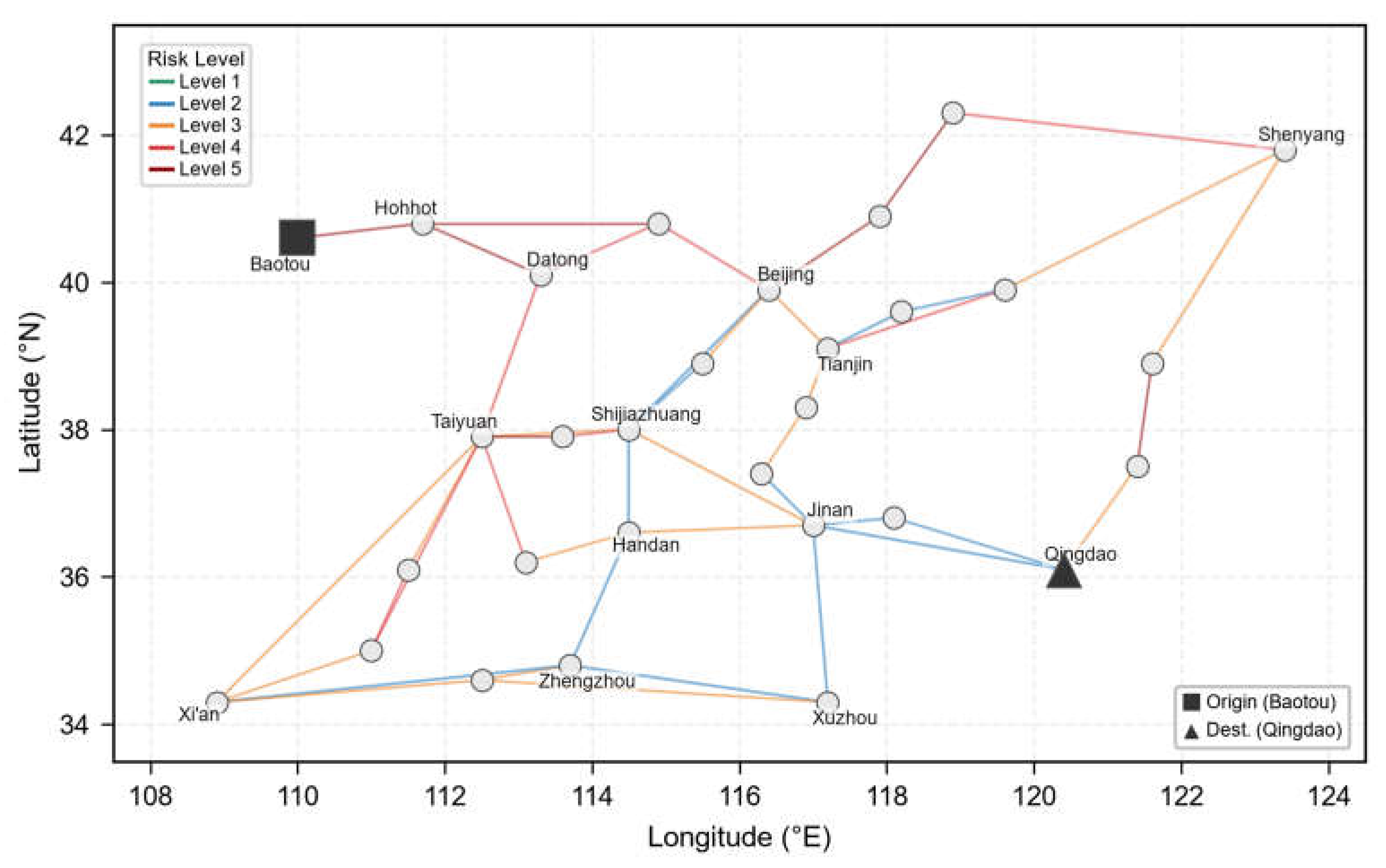
Figure 7.
Box-plot comparison of model performance under different uncertainty scenarios (S1–S5). Blue: deterministic model; Red: proposed robust model. (a) CVaR; (b) Gini coefficient; (c) Carbon emissions.
Figure 7.
Box-plot comparison of model performance under different uncertainty scenarios (S1–S5). Blue: deterministic model; Red: proposed robust model. (a) CVaR; (b) Gini coefficient; (c) Carbon emissions.
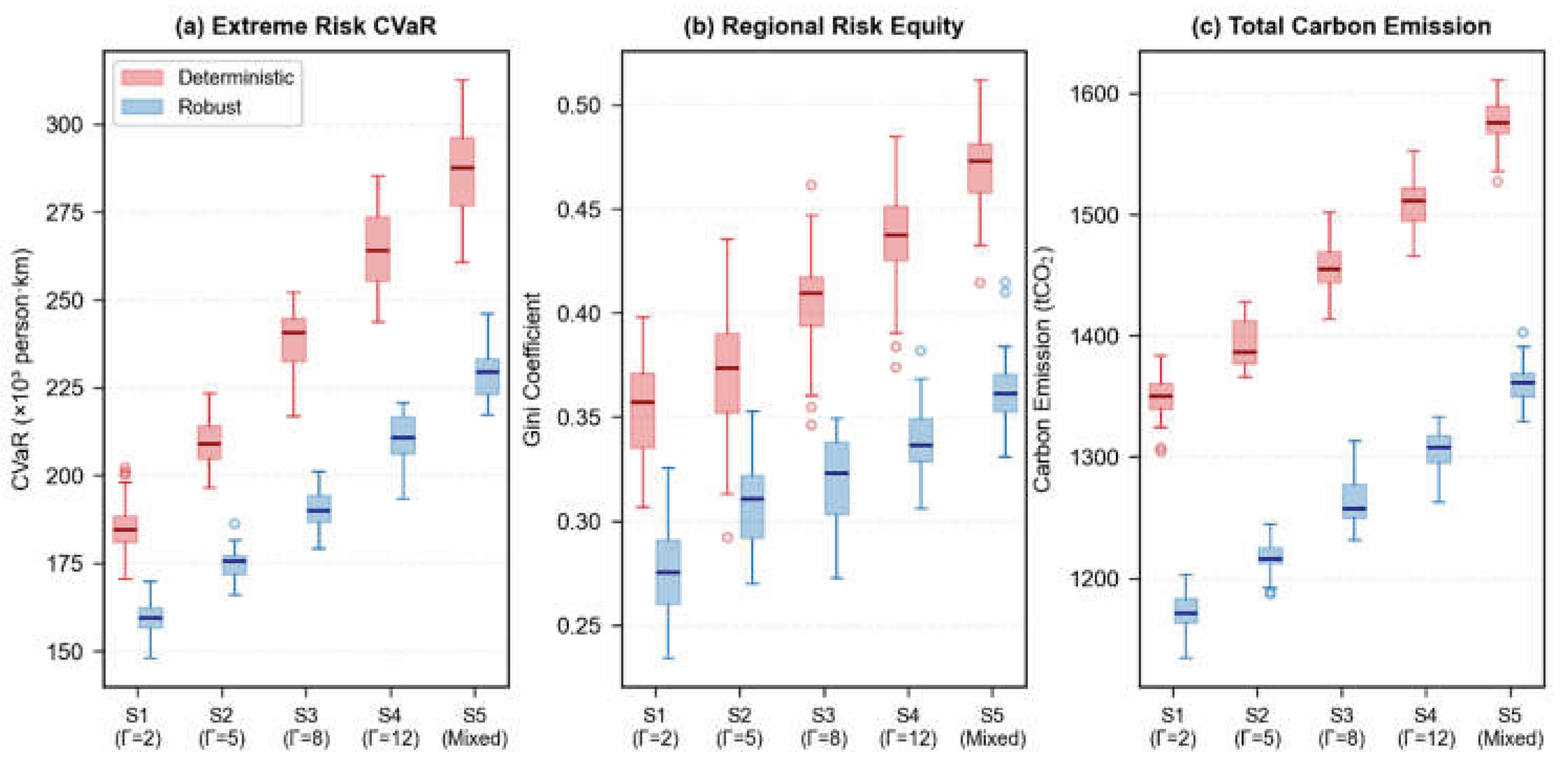
Table 2.
Network data and parameter configuration.
| parameter | Symbol | Dvalue/Range |
|---|---|---|
| Baseline accident probability | 1.2×10⁻⁸ to 8.5× 10⁻⁶ per km | |
| Cascading amplification factor | [1.0, 2.0] (remote uninhabited areas) [3.0, 8.0] (rural areas) [10.0, 20.0] (urban built-up shared lines) |
|
| Population exposure scale | Census township-level data + land-use remote sensing interpretation | |
| Traction carbon emission factor | 0.018-0.035 kgCO2/(t·km) (electried lines) 0.045-0.072 kgCO2/(t·km) (diesel-traction lines) |
|
| Maximum line throughput capacity | 3500-1200t/day | |
| OD pair | O→D | Baotou→Qingdao |
| Transport medium | — | Conventional flammable liquid (gasoline,benzene) |
| Nominal freight volume | q | 6000t |
| Peturbation magnitude | 20% of q(1200t) | |
| Robustness budget(baseline) | 5(traversed :{1,2,3,5,7,10,15}) | |
| CvaR confidence level | 0.95 |
Table 3.
ACE-NSGA-II algorithm parameter settings.
| Parameter | Value | Parameter | Value |
|---|---|---|---|
| Population size | 100 | Crossover range | [0.6, 0.9] |
| Max iterations | 200 | Mutation range | [0.05, 0.30] |
| Decay rate | 2.0 | Penalty coefficient | 10.0 |
| Penalty growth | 0.05 | Elite ratio | 0.10 |
| -shortest paths | 5 | CVaR confidence | 0.95 |
| Robust budget (base) | 5 | Perturbation | 20% |
Table 4.
Comprehensive algorithm performance comparison (mean standard deviation).
| Algorithm | IGD | HV | Spread | Time (s) |
|---|---|---|---|---|
| NSGA-II | ||||
| NSGA-III | ||||
| MOEA/D | ||||
| SPEA2 | ||||
| ACE-NSGA-II |
Table 5.
Bidirectional C-metric comparison across different freight volume levels.
| (t) | Forward | Reverse | ||||||||
|---|---|---|---|---|---|---|---|---|---|---|
| NSGA-II | NSGA-III | MOEA/D | SPEA2 | NSGA-II | NSGA-III | MOEA/D | SPEA2 | |||
| 2500 | 0.87 | 0.84 | 0.82 | 0.85 | 0.03 | 0.04 | 0.05 | 0.03 | ||
| 4500 | 0.88 | 0.85 | 0.83 | 0.86 | 0.02 | 0.03 | 0.04 | 0.03 | ||
| 6000 | 0.89 | 0.86 | 0.84 | 0.87 | 0.02 | 0.02 | 0.03 | 0.02 | ||
| 8000 | 0.87 | 0.85 | 0.82 | 0.86 | 0.03 | 0.04 | 0.04 | 0.03 | ||
Disclaimer/Publisher’s Note: The statements, opinions and data contained in all publications are solely those of the individual author(s) and contributor(s) and not of MDPI and/or the editor(s). MDPI and/or the editor(s) disclaim responsibility for any injury to people or property resulting from any ideas, methods, instructions or products referred to in the content. |
© 2026 by the authors. Licensee MDPI, Basel, Switzerland. This article is an open access article distributed under the terms and conditions of the Creative Commons Attribution (CC BY) license (http://creativecommons.org/licenses/by/4.0/).
Copyright: This open access article is published under a Creative Commons CC BY 4.0 license, which permit the free download, distribution, and reuse, provided that the author and preprint are cited in any reuse.


