A Sustainable Closed-Loop Supply Chain Design for Household Plastic Waste Considering Carbon Taxation and Regional Equity

1. Introduction

Household plastic waste management creates a decentralized closed-loop supply chain (CLSC) challenge because collection, recycling, and disposal decisions are spatially distributed [1]. Plastic products remain indispensable in household consumption, but global evidence on plastic production, waste accumulation, and international waste trade shows that their environmental consequences have become a major policy concern [2,3,4]. Low recycling rates, high sorting and disposal costs, and the uneven distribution of waste-management facilities jointly create a difficult CLSC design problem. Prior studies have emphasized the importance of reverse logistics, recycling capacity, and decentralized municipal solid waste management. However, two sustainability dimensions are still often treated as secondary add-ons rather than as structural parts of the model: carbon emissions and regional equity.

The CLSC design problem for household plastic waste differs from conventional product-remanufacturing settings [5]. Household plastic waste is generated locally and must be collected and sorted through region-specific systems [6,7,8,9], while disposal-facility or incineration expansion often faces political resistance [10,11]. Public sectors therefore face decentralized management costs that vary by region. At the same time, manufacturers decide how much recycled material to use based on cost, quality, and price competitiveness. When virgin plastic is cheaper or more reliable, recycling demand remains limited even if local public sectors can collect recyclable waste. These structural features motivate a bilevel model in which manufacturers and public sectors are separate decision makers.

A foundational treatment of closed-loop supply chain design that endogenized recycled-material prices through the interaction of public supply and manufacturer demand, while anchoring waste management in decentralized local operations [1], laid the initial groundwork for this class of problems. Yet the model is mainly organized around economic costs, real recycling rates, and decentralized operating burdens. In a policy environment where carbon taxation and regional fairness are increasingly relevant, the model can be extended in a sustainability direction.

This study develops that extension. We add carbon taxation to both the forward and reverse supply chain while assigning each emission source to one decision maker to avoid double counting. We also add a regional equity standard that limits the allowable deviation of regional disposal burdens from the average burden. This addition is not a cosmetic constraint: it changes the interpretation of the lower-level problem, because equity constraints couple local public sectors through a common social standard. The resulting structure is a regulated decentralized equilibrium.

The contributions of this study are threefold. First, we formulate a carbon-equity extension of a decentralized CLSC model for household plastic waste. Second, we show how carbon-cost derivatives and equity multipliers enter the mathematical program with equilibrium constraints (MPEC), avoiding the common but incorrect practice of adding a generic carbon term to every first-order condition. Third, we combine a reduced open-source MPEC/KKT validation with reproducible normalized policy simulations that compare carbon taxation, equity regulation, and combined policy scenarios in terms of real recycling rate (RRR), manufacturer profit, system emissions, public-sector cost, and regional cost dispersion.

The remainder of this paper is organized as follows. Section 2 reviews related literature. Section 3 presents the extended model, solution logic, and numerical experiment design. Section 4 reports the simulation results. Section 5 discusses policy implications and limitations. Section 6 concludes.

2. Literature Review

2.1. Closed-Loop Supply Chain Design for Plastic Waste

Closed-loop supply chain research examines how forward production and reverse recovery systems can be jointly designed. Across this literature, major themes include remanufacturing, collection channels, product return incentives, and sustainable reverse-logistics provider selection [5,12,13]. Household plastic waste creates a different setting because the reverse flow is not simply a customer product return. It is a municipal waste stream that requires sorting, collection, transfer, disposal, and sometimes interregional treatment.

Studies on municipal solid waste and reverse supply chain design have incorporated economic, environmental, and social dimensions. Some models optimize the location and allocation of waste facilities, while others evaluate waste separation, recycling capacity, and greenhouse gas emissions [6,7,8,9]. Lee and Chung [1] contribute to this literature by emphasizing local decentralized waste management and quantity-dependent pricing for plastic waste bales. The present paper uses that contribution as the base model and adds carbon taxation and regional equity as explicit sustainability instruments.

2.2. Carbon Management in CLSC and Waste Systems

Carbon policy affects CLSC design because virgin-resource use, product manufacturing, transportation, recycling, and disposal have different emission intensities. A carbon tax can alter relative costs between virgin and recycled materials and change the economics of recovery and remanufacturing [14,15]. Life-cycle evidence indicates that mechanically recycled plastic can have lower environmental impacts than comparable virgin plastic, although the magnitude depends on material quality, substitution, and system boundaries [25]. A carbon tax can therefore increase the price competitiveness of recycled inputs when this emissions advantage holds. Related robust and data-driven supply chain models show how implementation error and distributional ambiguity can be incorporated into operational decisions [16,17], but they do not address the carbon-equity coupling studied here. Recent Sustainability studies have examined carbon-policy responses, fairness-aware coordination, and government regulation in green CLSC systems [18,19,20]. However, carbon costs should be assigned carefully. If the manufacturer pays for recycled-bale emissions and public sectors also pay for the same transfer-station emissions, the model double counts the same physical emissions.

In waste systems, disposal emissions are especially relevant when incineration or landfill treatment is used. Collection and transport emissions are smaller but still important when interregional waste trade increases. Thus, a carbon-aware CLSC model should separate manufacturer emissions, public-sector operating emissions, and interregional trade emissions.

2.3. Regional Equity and Decentralized Waste Management

Waste management is inherently spatial. Disposal centers, incinerators, transfer stations, and collection routes impose local burdens. The “not in my backyard” problem reflects the fact that regional waste-management costs are not distributed evenly [10,11]. A policy that improves aggregate recycling may still be socially fragile if some regions bear disproportionate disposal costs.

Regional equity can be modeled in multiple ways: maximum cost deviation, minimum service level, compensation, facility burden-sharing, or social fairness objectives. Fairness concerns have also been studied in closed-loop supply chain coordination under carbon-neutral reward and punishment mechanisms [19]. This paper uses a proportional burden-deviation standard. The standard is transparent and easy to interpret: each region’s disposal burden must remain within a specified percentage of the average regional disposal burden. A smaller threshold represents a stricter equity requirement.

3. Materials and Methods

3.1. Base Network, Sets, and Decision Structure

The extended model keeps the leader-follower structure of the source paper. The manufacturer is the leader and chooses virgin-resource purchases, recycled-bale purchases, and product shipments. Public sectors are followers and choose local collection, third-party purchases, transfer-station bale production, disposal, capacity expansion, and interregional disposal trade. The extension adds two policy instruments without changing the basic hierarchy: a carbon tax $T$ and a regional equity threshold $U$.

Let $S$, $M$, $I$, $V$, and $N$ denote suppliers, manufacturing plants, customer/public-sector regions, recycled-bale types, and grid points used for piecewise price approximation. The upper-level decision vector is:

$${\mathbf{x}}^M=\{X_{sm},Y_{imv},W_{mi},Q_{imvn}:s\in S,m\in M,i\in I,v\in V,n\in N\}.$$

(1)

The lower-level decision vector of public sector $i$ is:

$${\mathbf{x}}_i^P=\{z_i^c,x_i^c,z_i^{cd},x_i^{cd},z_{iv}^{cm},z_i^{cc},z_{ij}^{dd},q_i^d:j\in I,v\in V\}.$$

(2)

The physical meaning of the main variables follows the reference model: $X_{sm}$ is virgin plastic purchased by plant $m$ from supplier $s$, $Y_{imv}$ is type $v$ recycled bale purchased by plant $m$ from public sector $i$, and $W_{mi}$ is product shipment from plant $m$ to customer region $i$. In the public-sector block, $z_i^c$ and $x_i^c$ are recyclable waste collected from collection centers and third parties, $z_i^{cd}$ and $x_i^{cd}$ are non-recyclable waste flows, $z_{iv}^{cm}$ is compressed bale production, $z_i^{cc}$ is residual waste shipped from the transfer station to disposal, $z_{ij}^{dd}$ is disposal trade from $i$ to $j$, and $q_i^d$ is additional disposal operation.

3.2. Manufacturer Model with Quantity-Dependent Prices and Carbon Taxation

The recycled-bale purchasing price retains the nonlinear quantity-dependent structure of Lee and Chung [1]. For public sector $i$ and bale type $v$, the price charged to the manufacturer is:

$$C_{iv}=f_{iv}^C\left(z_{iv}^{cm},Y_{\cdot iv}\right)={\alpha }_{iv}^{cm}-{\beta }_{iv}^{cm}{\left(z_{iv}^{cm}\right)}^t+{\gamma }_{iv}^{cm}{\left(\sum _{m\in M}{Y}_{imv}\right)}^t, i\in I,\hspace{0.25em}v\in V.$$

(3)

The purchase-cost term is nonlinear because $C_{iv}{Y}_{imv}$ contains both the price and the purchased quantity:

$$C_{iv}{Y}_{imv}=f_{iv}^C\left(z_{iv}^{cm},Y_{\cdot iv}\right)Y_{imv}, i\in I,\hspace{0.25em}m\in M,\hspace{0.25em}v\in V.$$

(4)

Following the reference paper, the nonlinear cost is approximated by an SOS1 grid. Let ${\Delta }_{imvn}$ be grid-point quantity and $g_{imvn}$ be the cost value at grid point $n$:

$$g_{imvn}=f_{iv}^C\left(z_{iv}^{cm},{\Delta }_{imvn}\right){\Delta }_{imvn}, i\in I,\hspace{0.25em}m\in M,\hspace{0.25em}v\in V,\hspace{0.25em}n\in N.$$

(5)

The approximation is:

$$C_{iv}{Y}_{imv}\approx \sum _{n\in N}{g}_{imvn}{Q}_{imvn}, i\in I,\hspace{0.25em}m\in M,\hspace{0.25em}v\in V,$$

(6)

$$\sum _{n\in N}{Q}_{imvn}\le 1, \sum _{n\in N}{\Delta }_{imvn}{Q}_{imvn}=Y_{imv}, Q_{imvn}\in \{\mathrm{0,1}\}.$$

(7)

Let $E_s^N$, $E_{iv}^R$, and $E_{mi}^W$ be emission factors for virgin plastic resources, recycled-bale use, and product transportation. The manufacturer carbon account is:

$$C^M({\mathbf{x}}^M)=\sum _{s\in S}\sum _{m\in M}{E}_s^N{X}_{sm}+\sum _{i\in I}\sum _{m\in M}\sum _{v\in V}{E}_{iv}^R{Y}_{imv}+\sum _{m\in M}\sum _{i\in I}{E}_{mi}^W{W}_{mi}.$$

(8)

The upper-level problem is written in component form to keep the revenue, input-cost, piecewise purchasing-cost, production-cost, and carbon-cost terms transparent:

$$\underset{{\mathbf{x}}^M}{\max }\hspace{0.25em}{\pi }^T={\Pi }^R-{\Pi }^N-{\Pi }^B-{\Pi }^G-{\Pi }^P-T{C}^M({\mathbf{x}}^M).$$

(9)

$${\Pi }^R=\sum _{m\in M}\sum _{i\in I}{P}_i{W}_{mi}.$$

(10)

$${\Pi }^N=\sum _{s\in S}\sum _{m\in M}{C}_s{X}_{sm}+\sum _{s\in S}\sum _{m\in M}{K}_s{X}_{sm}.$$

(11)

$${\Pi }^B=\sum _{i\in I}\sum _{m\in M}\sum _{v\in V}{K}_i{Y}_{imv}.$$

(12)

$${\Pi }^G=\sum _{i\in I}\sum _{m\in M}\sum _{v\in V}\sum _{n\in N}{g}_{imvn}{Q}_{imvn}.$$

(13)

$${\Pi }^P=\sum _{m\in M}\sum _{i\in I}{C}_m{W}_{mi}.$$

(14)

The manufacturer is subject to material balance, demand, sourcing capacity, maximum bale supply, recycling-policy, and SOS1 constraints:

$$\sigma \sum _{s\in S}{X}_{sm}+\sum _{i\in I}\sum _{v\in V}{Y}_{imv}=\sum _{i\in I}{W}_{mi}, m\in M,$$

(15)

$$\sum _{m\in M}{W}_{mi}=D_i, i\in I,$$

(16)

$$\sum _{m\in M}{X}_{sm}\le CA{P}_s, \sum _{m\in M}\sum _{v\in V}{Y}_{imv}\le CA{P}_i,$$

(17)

$$\sum _{m\in M}{Y}_{imv}\le z_{iv}^{cm}, i\in I,\hspace{0.25em}v\in V,$$

(18)

$$\sum _{i\in I}\sum _{m\in M}\sum _{v\in V}{Y}_{imv}\ge R\sum _{i\in I}{D}_i,$$

(19)

$$X_{sm}\ge 0, Y_{imv}\ge 0, W_{mi}\ge 0.$$

(20)

The carbon tax changes relative input costs through the marginal term $T(E_s^N-E_{iv}^R)$. When virgin-resource emissions exceed recycled-bale emissions, a higher $T$ increases the shadow value of recycled-bale capacity.

3.3. Public-Sector Model with Carbon and Regional Equity

The source PDF writes the public-sector objective using $\max {\varphi }_i^{tot}$, but the surrounding text and KKT equations describe cost minimization. This paper therefore treats the objective direction as a typographical error and uses cost minimization. Public sector $i$ minimizes:

$$\underset{{\mathbf{x}}_i^P}{\min }\hspace{0.25em}{\varphi }_i^T={\varphi }_i^{cc}+{\varphi }_i^{ts}+{\varphi }_i^d+T{C}_i^P.$$

(21)

The collection-center cost block is:

$${\varphi }_i^{cc}=c_i^c{z}_i^c+e_i^c{z}_i^c+p_i^c{x}_i^c+c_i^c{z}_i^{cd}+e_i^c{z}_i^{cd}+p_i^{cd}{x}_i^{cd},$$

(22)

with flow and participation constraints:

$$z_i^c+x_i^c=O_i{\theta }_i, z_i^{cd}+x_i^{cd}=O_i(1-{\theta }_i),$$

(23)

$$(p_i^c-c_i^c)x_i^c\ge 0, (p_i^{cd}-c_i^c)x_i^{cd}\ge 0.$$

(24)

The third-party recyclable-waste price is represented with two compact power terms:

$$p_i^c=f_i^p(O_i,Y_{i\cdot \cdot })={\alpha }_i^D-{\beta }_i^D{H}_i^D+{\gamma }_i^D{G}_i^D.$$

(25)

$$H_i^D={\theta }_i^t{O}_i^t.$$

(26)

$$G_i^D={\left(\sum _{m\in M}\sum _{v\in V}{Y}_{imv}\right)}^t.$$

(27)

The transfer-station unit processing cost is:

$$k_{iv}^{ts}=c_{iv}^{cc}+c_{iv}^p+I{n}_i^{cc}.$$

(28)

The transfer-station cost block is:

$${\varphi }_i^{ts}=c_i^{cl}{O}_i{\theta }_i+\sum _{v\in V}{k}_{iv}^{ts}{z}_{iv}^{cm},$$

(29)

subject to:

$$z_{iv}^{cm}\le (x_i^c+z_i^c)(1-{\tau }_1){\tau }_{2v}, i\in I,\hspace{0.25em}v\in V,$$

(30)

$$z_{iv}^{cm}\ge \sum _{m\in M}{Y}_{imv}, \sum _{v\in V}{z}_{iv}^{cm}+z_i^{cc}=x_i^c+z_i^c.$$

(31)

The actual disposal quantity is:

$$D_i^{disp}=z_i^{cc}+z_i^{cd}+x_i^{cd}-\sum _{j\in I}{z}_{ij}^{dd}+\sum _{j\in I}{z}_{ji}^{dd}.$$

(32)

Define $B_i^d=c_i^d+e_i^d$ and $S_{ij}^{tr}=(1+tax)c_j^{se}$. The disposal-center cost block is:

$${\varphi }_i^d=B_i^d{D}_i^{disp}+\sum _{j\in I}{S}_{ij}^{tr}{z}_{ij}^{dd}-\sum _{j\in I}{c}_i^{se}{z}_{ji}^{dd}+q_i^d.$$

(33)

The disposal-capacity, trade-limit, and budget constraints are:

$$D_i^{disp}\le CA{P}_i^d+a_i{q}_i^d, \sum _{j\in I}{z}_{ij}^{dd}\le z_i^{cc}+z_i^{cd}+x_i^{cd},$$

(34)

$$q_i^d\le b, z_i^c,x_i^c,z_i^{cd},x_i^{cd},z_i^{cc},z_{iv}^{cm},z_{ij}^{dd},q_i^d\ge 0.$$

(35)

The public-sector carbon account assigns collection, bale production, disposal, and interregional trade emissions to public sectors:

$$C_i^P({\mathbf{x}}_i^P)=E_i^C(z_i^c+x_i^c+z_i^{cd}+x_i^{cd})+\sum _{v\in V}{E}_{iv}^B{z}_{iv}^{cm}+E_i^D{D}_i^{disp}+\sum _{j\in I}{E}_{ij}^{TR}{z}_{ij}^{dd}.$$

(36)

Regional equity is modeled as a proportional bound on disposal-burden deviation. Let $N_I$ denote the number of public-sector regions and let ${\mu }^d$ denote the average disposal burden. Define:

$${\mu }^d=N_I^{-1}\sum _{i\in I}{\varphi }_i^d.$$

(37)

The equity standard is:

$${\varphi }_i^d-(1+U){\mu }^d\le 0, (1-U){\mu }^d-{\varphi }_i^d\le 0, i\in I.$$

(38)

The threshold $U\in \left[\mathrm{0,1}\right]$ is the maximum allowed proportional deviation from the average disposal burden. A smaller $U$ represents stricter equity regulation.

3.4. MPEC Reformulation and Local Algebraic Claims

The lower-level public-sector problems are transformed into first-order optimality, primal feasibility, dual feasibility, and complementarity conditions. Let ${\lambda }_i^r$ denote multipliers for local constraints and let ${\eta }_i^U$ and ${\eta }_i^L$ denote the upper- and lower-deviation equity multipliers. Define the equity residuals:

$$A_i^U={\varphi }_i^d-(1+U){\mu }^d.$$

(39)

$$A_i^L=(1-U){\mu }^d-{\varphi }_i^d.$$

(40)

The regulated lower-level Lagrangian can be written compactly as:

$${\mathcal{L}}_i={\varphi }_i^T+\sum _r{\lambda }_i^r{g}_i^r({\mathbf{x}}_i^P;{\mathbf{x}}^M)+{\eta }_i^U{A}_i^U+{\eta }_i^L{A}_i^L.$$

(41)

For any public-sector variable $u_i$, the stationarity condition is:

$${\displaystyle \frac{\partial {\varphi }_i}{\partial u_i}}+T{\displaystyle \frac{\partial C_i^P}{\partial u_i}}+\sum _r{\lambda }_i^r{\displaystyle \frac{\partial g_i^r}{\partial u_i}}+{\Omega }_i(u_i)=0,$$

(42)

where the equity-gradient correction is:

$${\Omega }_i(u_i)=M_i^{\eta }{\displaystyle \frac{\partial {\varphi }_i^d}{\partial u_i}}.$$

(43)

$$B^{\eta }=\sum _{h\in I}\left[(1+U){\eta }_h^U-(1-U){\eta }_h^L\right].$$

(44)

$$M_i^{\eta }={\eta }_i^U-{\eta }_i^L-N_I^{-1}{B}^{\eta }.$$

(45)

This term is zero for variables that do not affect the disposal-burden block and nonzero for disposal, capacity, and trade variables. The selective carbon derivatives are:

$${\displaystyle \frac{\partial C_i^P}{\partial z_i^c}}=E_i^C, {\displaystyle \frac{\partial C_i^P}{\partial z_{iv}^{cm}}}=E_{iv}^B, {\displaystyle \frac{\partial C_i^P}{\partial D_i^{disp}}}=E_i^D, {\displaystyle \frac{\partial C_i^P}{\partial z_{ij}^{dd}}}=E_{ij}^{TR}.$$

(46)

Representative stationarity equations are:

$$c_i^c+e_i^c+T{E}_i^C-p_i^c-{\lambda }_i^1-\sum _{v\in V}{\lambda }_{iv}^5(1-{\tau }_1){\tau }_{2v}+{\lambda }_i^7-{\lambda }_i^{11}=0,$$

(47)

$$c_{iv}^{cc}+c_{iv}^p+I{n}_i^{cc}+T{E}_{iv}^B+{\lambda }_{iv}^5-{\lambda }_{iv}^6-{\lambda }_i^7-{\lambda }_{iv}^{13}=0,$$

(48)

$$c_i^d+e_i^d+T{E}_i^D-{\lambda }_i^7+{\lambda }_i^8-{\lambda }_i^9-{\lambda }_i^{14}+{\Omega }_i\left(D_i^{disp}\right)=0,$$

(49)

$$(1+tax)c_j^{se}+T{E}_{ij}^{TR}+{\lambda }_i^9-{\lambda }_{ij}^{17}+{\Omega }_i\left(z_{ij}^{dd}\right)=0,$$

(50)

$$1-a_i{\lambda }_i^8+{\lambda }_i^{10}-{\lambda }_i^{18}=0.$$

(51)

The complementarity block is:

$$0\le {\lambda }_i^r\perp g_i^r({\mathbf{x}}_i^P;{\mathbf{x}}^M)\ge 0, 0\le {\eta }_i^U\perp (1+U){\mu }^d-{\varphi }_i^d\ge 0,$$

(52)

$$0\le {\eta }_i^L\perp {\varphi }_i^d-(1-U){\mu }^d\ge 0, i\in I.$$

(53)

The full single-level MPEC is therefore:

$$\underset{{\mathbf{x}}^M,{\mathbf{x}}^P,\lambda ,\eta }{\max }\hspace{0.25em}{\pi }^T.$$

(54)

$${\mathbf{x}}^M\in {\mathcal{X}}^M, {\mathbf{x}}^P\in {\mathcal{X}}^P\left({\mathbf{x}}^M\right).$$

(55)

$${\nabla }_{{\mathbf{x}}^P}\mathcal{L}({\mathbf{x}}^P,\lambda ,\eta ;{\mathbf{x}}^M)=0.$$

(56)

$$0\le \lambda \perp g({\mathbf{x}}^P;{\mathbf{x}}^M)\ge 0.$$

(57)

$$0\le {\eta }^U\perp (1+U){\mu }^d-{\varphi }^d\ge 0.$$

(58)

$$0\le {\eta }^L\perp {\varphi }^d-(1-U){\mu }^d\ge 0.$$

(59)

Lemma 1.

Carbon taxation enters each KKT stationarity equation only through the derivative of the emission block physically assigned to that variable.

Proof. 

Since $C_i^P$ is additively separable into collection, bale-production, disposal, and trade terms, $\partial C_i^P/\partial u_i$ equals the relevant emission factor if $u_i$ appears in that block and equals zero otherwise. Therefore, a generic carbon term cannot be added to every stationarity equation without double counting or assigning emissions to unrelated variables. □

Lemma 2.

The equity standard converts the independent public-sector follower system into a regulated decentralized equilibrium.

Proof. 

Without the equity standard, ${\mathcal{L}}_i$ contains only local costs and local constraints conditional on the manufacturer’s $Y_{imv}$. With the equity standard, ${\mu }^d$ contains all public sectors’ disposal burdens, and ${\Omega }_i\left(u_i\right)$ depends on the vector of equity multipliers $\{{\eta }_h^U,{\eta }_h^L{\}}_{h\in I}$. Hence each local stationarity system is coupled through the common burden benchmark. □

3.5. Computational Validation and Numerical Experiment Design

The computational design has two layers. The first layer is a reduced continuous MPEC/KKT validation with six public-sector regions. It keeps the same economic mechanism as the analytical model: quantity-dependent recycled-bale prices, a manufacturer choice between virgin and recycled inputs, public-sector recycling and disposal decisions, carbon taxation, and regional equity bounds. The manufacturer problem is solved with SciPy’s bounded scalar optimizer over total recycled purchases, and region-level purchases are allocated to the lowest effective recycled-bale costs. Conditional on the manufacturer’s decision, the public-sector problem is solved with SLSQP after a linear-programming feasibility initialization. The implied lower-level KKT system is then checked by non-negative least-squares recovery of active multipliers. The reduced validation omits the SOS1 binary grid-selection structure and evaluates the continuous KKT core of the extension. It therefore establishes local algebraic and numerical feasibility rather than equivalence in global optimality or computational performance to the full Gurobi-based mixed-integer formulation. This validation is deliberately smaller than the full model, but it is a genuine open-source optimization calculation rather than a spreadsheet-style scenario simulation.

The second layer is a twelve-region calibrated policy simulation. This layer includs region-level waste volumes, sorting rates, transfer-station conversion, collection costs, disposal costs, and recycled-bale price functions. The simulation is used for the full carbon-equity scenario grid and for Figure 1, Figure 2, Figure 3, Figure 4, Figure 5, Figure 6 and Figure 7. The two-layer design separates computational validity from policy visualization: the reduced optimization layer shows that the MPEC/KKT extension is numerically implementable, while the calibrated simulation layer provides transparent comparative-static evidence for the larger regional setting. The reduced validation should therefore be read as a convergence and mechanism test. It verifies that the selective carbon-tax KKT terms and the equity-coupled public-sector conditions can be solved with small residuals in a continuous setting; it is not used as a substitute for the twelve-region policy grid or for a full mixed-integer MPEC with SOS1 binaries.

The simulation evaluates three experiment groups:

Experiment 1.

baseline scenario with no carbon tax and no equity standard.

Experiment 2.

carbon-tax scenarios with $T=\mathrm{0,10,20,30,40,50}$ USD/tCO2.

Experiment 3.

combined carbon-equity scenarios with $T=30$ USD/tCO2 and $U=5\%,10\%,15\%,20\%,25\%$.

The main performance indicators are real recycling rate (RRR), manufacturer profit, total system emissions, public-sector cost, and the standard deviation of regional management costs. The Python simulation code, optimization-validation code, output tables, figures, and residual-verification logs are provided with the manuscript package. The verification modules check feasibility residuals, supply-capacity slack, lower-level KKT stationarity, complementarity, carbon-tax monotonicity for RRR, profit, and emissions, and the main equity proposition comparing strict and loose equity thresholds.

The emission parameters are shown in Table 1. They are normalized scenario values rather than claim-specific lifecycle measurements. The source column identifies the empirical basis used to set a plausible order of magnitude from waste-accounting, lifecycle-inventory, recycled-plastic LCA, and freight-conversion sources [21,22,23,25]; an applied case study should replace these values with plastic-type- and region-specific lifecycle inventory data. The carbon-tax range and emission factors should therefore be interpreted as scenario levers rather than transferable policy estimates, particularly for developing economies with different energy mixes, collection systems, disposal technologies, and enforcement capacities.

Table 2 reports the reduced optimization validation. Carbon taxation raises the optimized recycled share from 20.00% to 24.65%, while manufacturer profit decreases from 0.384 million USD to 0.307 million USD. In the carbon-tax scenario, imposing a strict equity threshold reduces regional disposal-burden dispersion from 19.37 thousand USD to 0.00 thousand USD in the reduced lower-level system. This near-zero dispersion is a boundary outcome of the stylized six-region continuous validation, where a tight 5% equity band and feasibility initialization make the burden-equalization constraints binding. It should not be interpreted as a prediction that equity policy eliminates regional inequality in the full setting. In the twelve-region policy simulation, the same strict equity threshold lowers regional cost dispersion to 23.23 thousand USD rather than zero. The lower-level KKT stationarity, complementarity, and primal-feasibility residuals are all below ${10}^{-6}$.

4. Results

4.1. Carbon Taxation

The baseline level should be interpreted as a calibrated extension baseline rather than a direct reproduction of a single scenario in Lee and Chung [1]. In the source paper, Table 9 reports RRR values of 11.58% at the 100% increase-rate case for both S1 and S2, with maximum values of 17.4% in S1 and 22.4% in S2; the government-policy analysis also reports an unconstrained recycling level of about 11.6%. The 25.02% baseline in this paper is generated by the extended carbon-equity calibration and is used to compare policy movements within the new model.

Figure 1 reports the effect of carbon taxation on the real recycling rate. In the baseline scenario, the RRR is 25.02%. Introducing a carbon tax of 10 USD/tCO2 increases the RRR to 28.09%. Further tax increases do not raise the RRR because the recycled-bale supply capacity becomes binding. This pattern is important: carbon taxation can stimulate recycled input demand, but only when reverse-supply capacity is available.

Figure 1. Carbon tax and real recycling rate.

Figure 1. Carbon tax and real recycling rate.

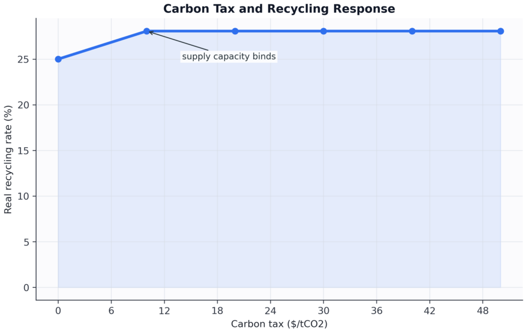
Figure 2 shows manufacturer profit under carbon taxation. Profit declines from 3.65 million USD in the baseline to 2.50 million USD at 50 USD/tCO2. This decline occurs because carbon taxation raises the cost of both virgin and recycled inputs, even though recycled inputs become relatively more attractive. The result highlights a policy trade-off: a tax can improve recycling and emissions performance, but it can also reduce manufacturer profitability if no complementary recycling subsidy is provided.

Figure 2. Carbon tax and manufacturer profit.

Figure 2. Carbon tax and manufacturer profit.

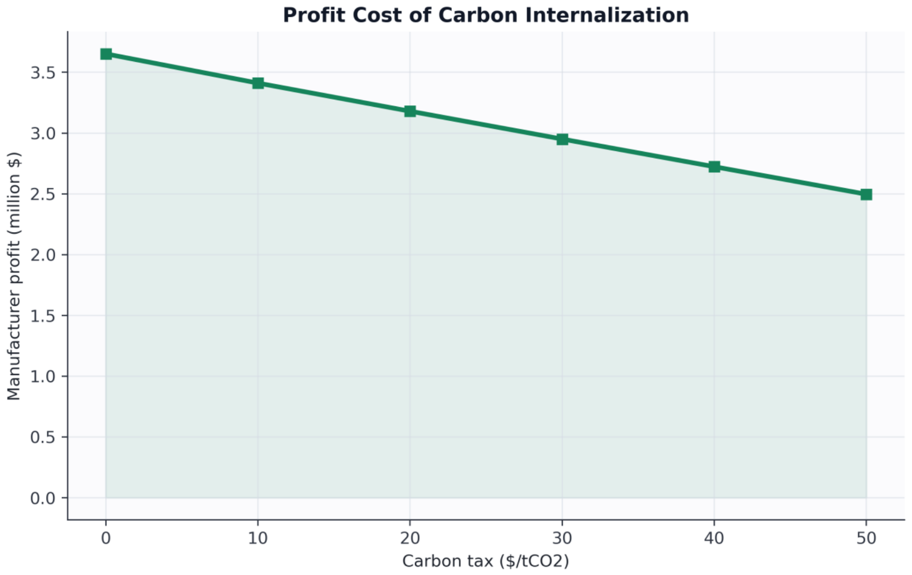
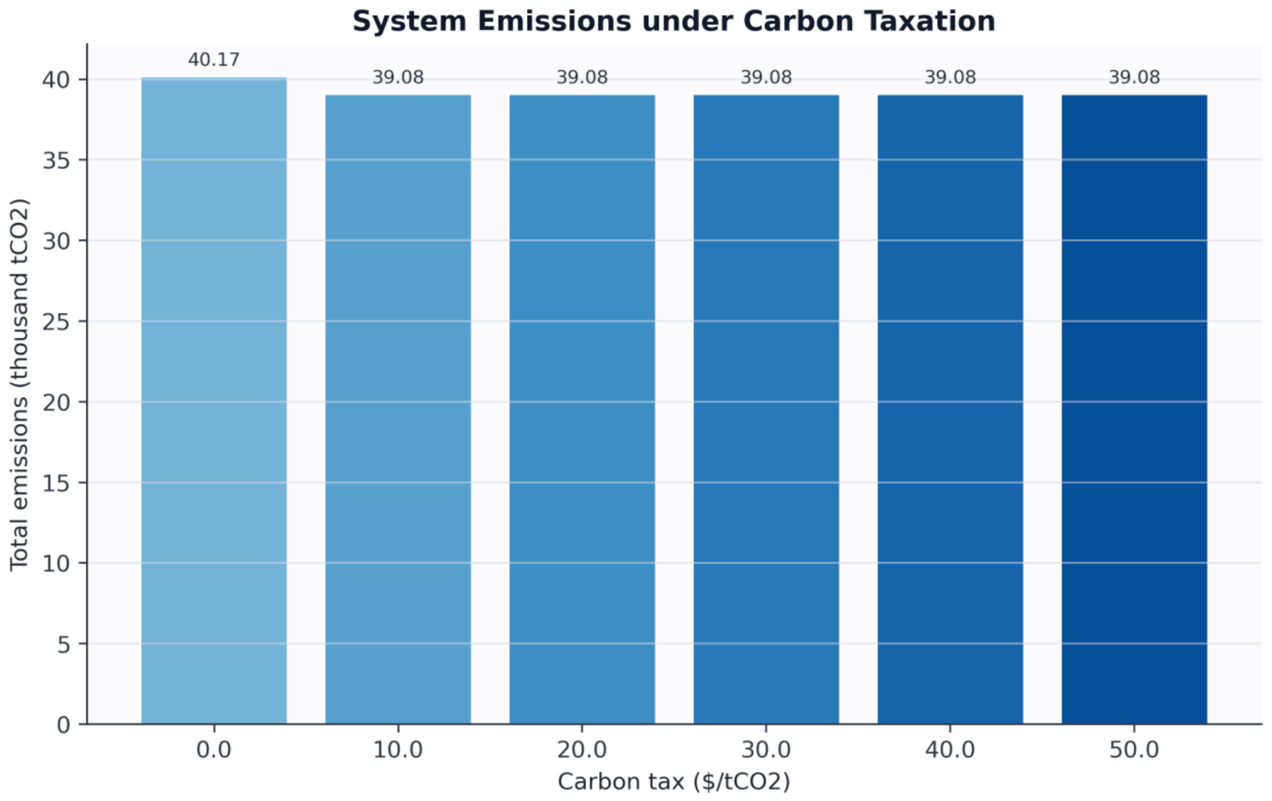
Figure 3 shows total system emissions. Emissions decline from 40.17 thousand tCO2 in the baseline to 39.08 thousand tCO2 once recycled-bale use reaches the supply limit. This is a 2.73% reduction. The plateau after 10 USD/tCO2 confirms that emissions reduction becomes constrained by recycled-bale availability rather than by the carbon tax rate itself.

Figure 3. Carbon tax and system emissions.

Figure 3. Carbon tax and system emissions.

4.2. Regional Equity

Figure 4 reports the relationship between the equity threshold $U$ and the RRR at a carbon tax of 30 USD/tCO2. A stricter equity standard, represented by a lower $U$, slightly raises the RRR because recycling effort is redirected toward high-burden regions. When $U=5\%$, the RRR reaches 28.58%; when $U=25\%$, it returns to approximately the no-equity value of 28.09%.

Figure 4. Equity threshold and real recycling rate.

Figure 4. Equity threshold and real recycling rate.

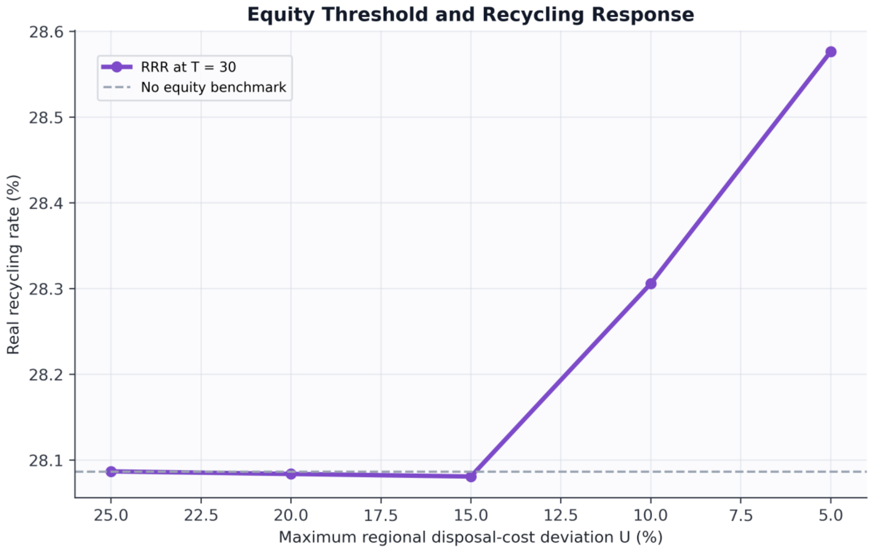
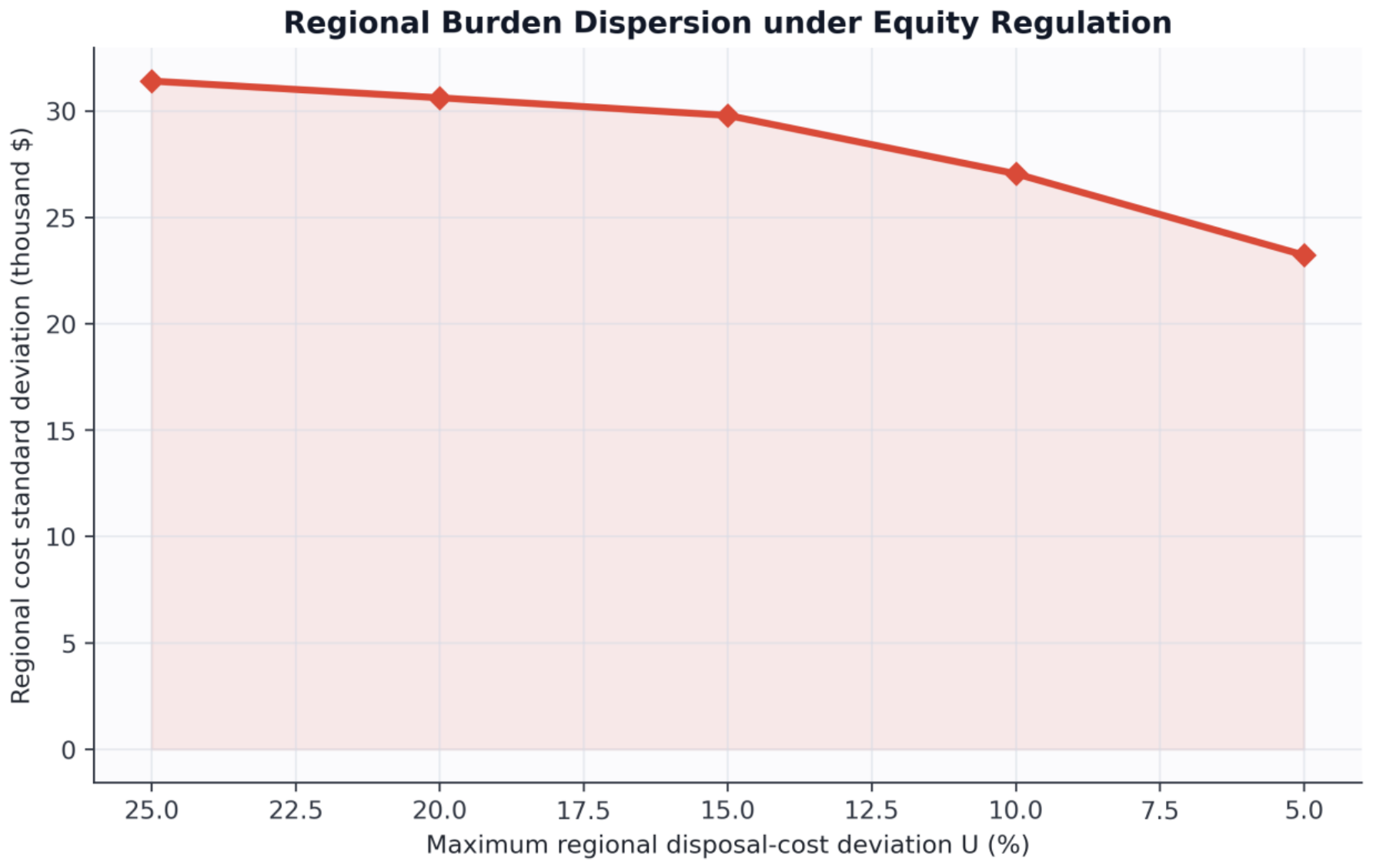
Figure 5 shows the effect of equity standards on regional cost dispersion. Tightening $U$ from 25% to 5% reduces the regional cost standard deviation from 31.41 thousand USD to 23.23 thousand USD, a reduction of approximately 26.1%. This confirms that equity standards can mitigate regional burden inequality, even though they require administrative coordination and targeted capacity support.

Figure 5. Equity threshold and regional cost dispersion.

Figure 5. Equity threshold and regional cost dispersion.

4.3. Carbon-Equity Policy Frontier

Figure 6 plots the combined-policy frontier. The horizontal axis is system emissions, the vertical axis is regional cost dispersion, and point color represents the real recycling rate. The frontier illustrates that carbon and equity policies are not substitutes. Carbon taxation primarily moves the system toward lower emissions and higher recycled-bale adoption, whereas equity standards primarily lower regional cost dispersion. The best policy region in the simulation combines a positive carbon tax with a strict but feasible equity standard.

Figure 6. Carbon-equity policy frontier.

Figure 6. Carbon-equity policy frontier.

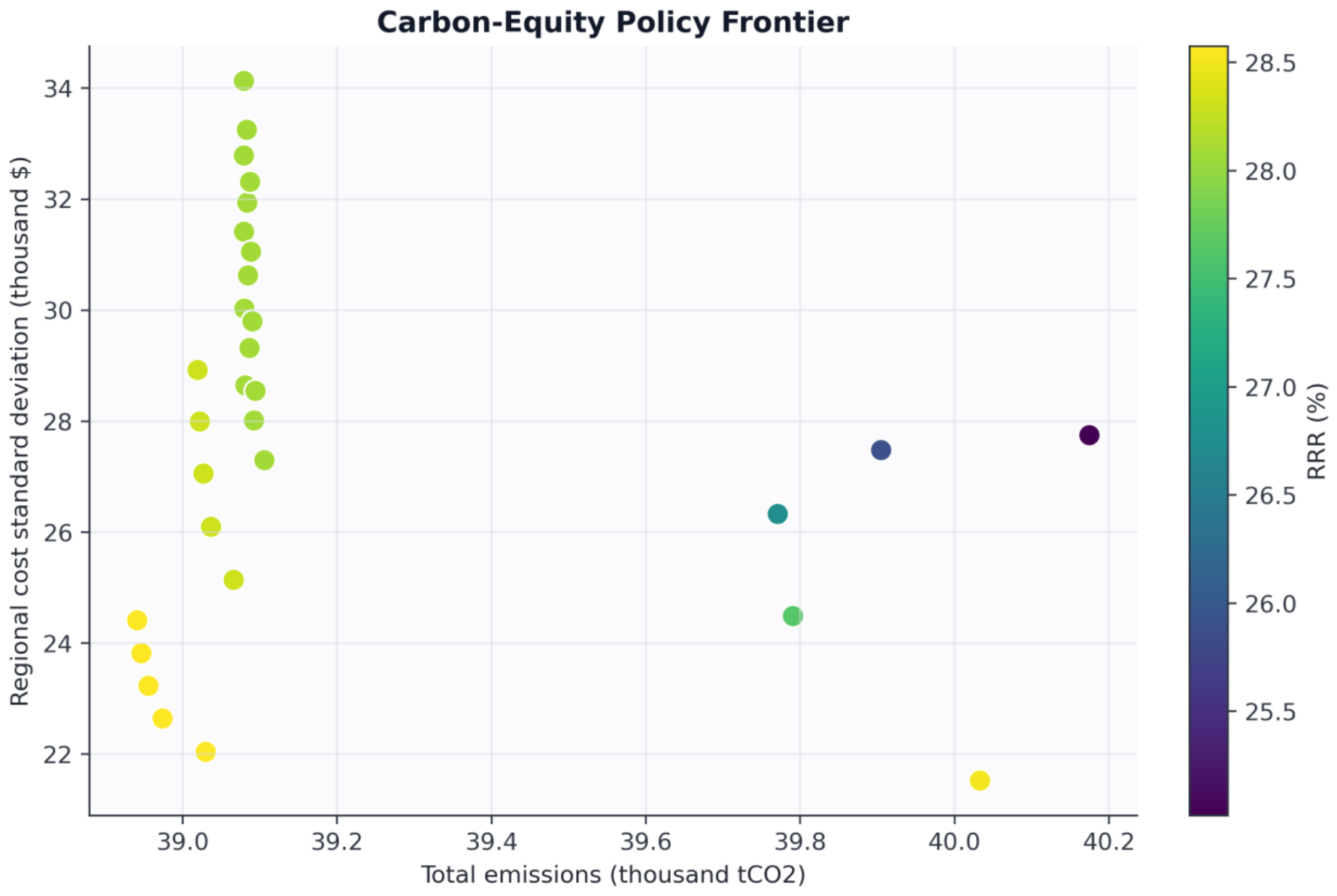
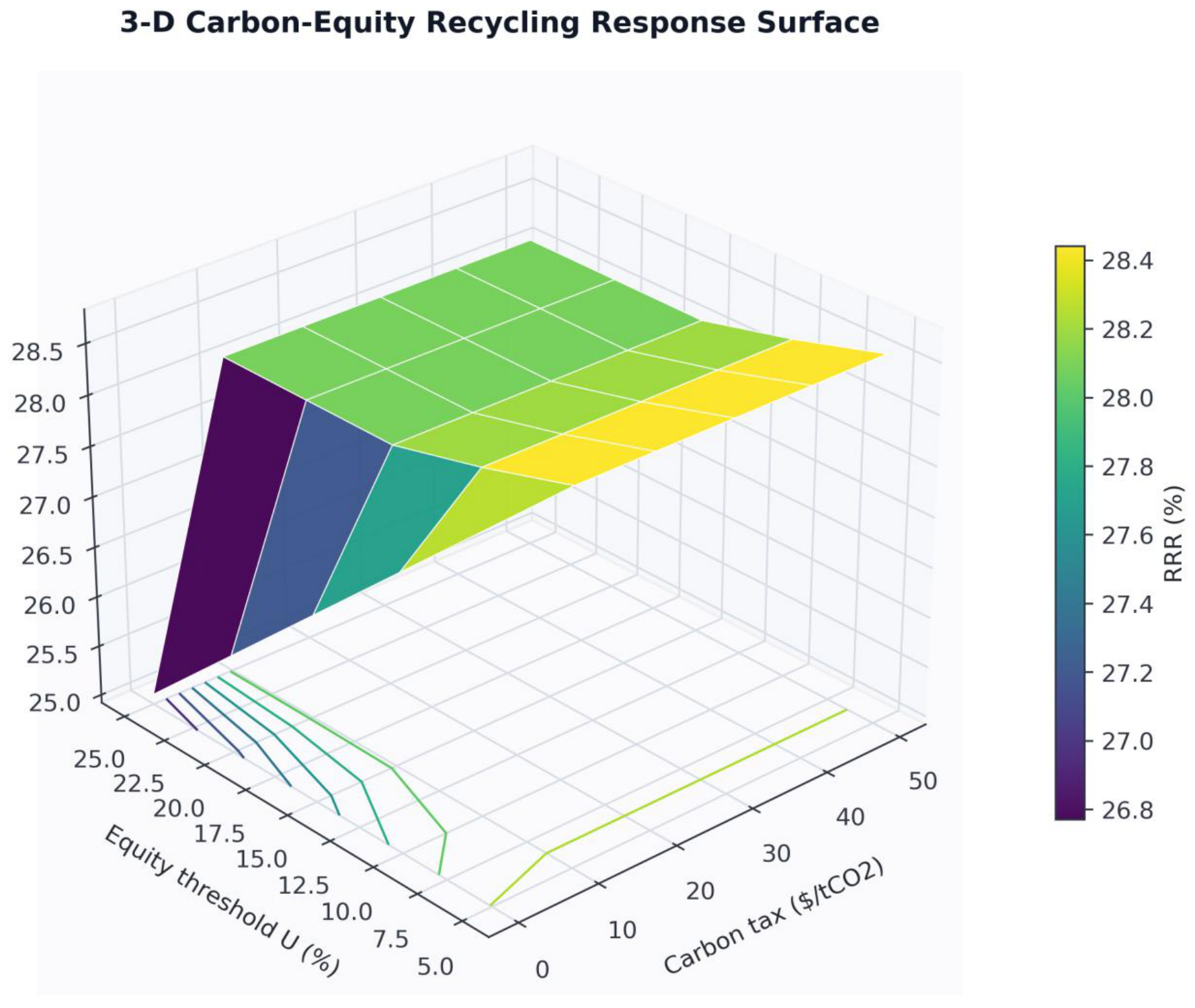
Figure 7 provides a three-dimensional response surface for the same combined-policy grid. The surface makes the policy interaction clearer than a two-dimensional frontier alone. The carbon-tax axis raises the RRR sharply when the tax moves from zero to a positive level, whereas the equity axis creates an additional uplift when $U$ becomes strict. The flat segment at higher tax rates confirms that the marginal carbon-tax effect is limited by recycled-bale supply capacity.

Figure 7. Three-dimensional carbon-equity response surface for real recycling rate.

Figure 7. Three-dimensional carbon-equity response surface for real recycling rate.

The residual-verification routine reports zero residuals for all tested propositions under a tolerance of ${10}^{-6}$. The simulation log concludes that all proposition checks passed, and the optimization-validation log concludes that all optimization-validation checks passed. Together, these checks confirm that the numerical outputs used in Figure 1, Figure 2, Figure 3, Figure 4, Figure 5, Figure 6 and Figure 7 and Table 3 are internally consistent with the reported comparative-static claims and with the reduced lower-level KKT conditions.

Table 3 summarizes representative full-scale simulation scenarios.

5. Discussion

5.1. Policy Implications

The results generate three policy implications.

First, carbon taxation is effective only up to the point at which recycled-bale supply becomes binding. In the simulation, even a moderate tax of 10 USD/tCO2 is enough to make recycled bales more attractive, but higher taxes do not increase recycling unless local collection and transfer-station capacity expand. This suggests that carbon taxes should be paired with investment in reverse-supply capacity.

Second, regional equity standards address a different policy failure. Carbon taxation internalizes emissions, but it can leave disposal burdens unevenly distributed across public sectors. A regional equity standard reduces burden dispersion and may strengthen recycling in high-cost regions. This supports a policy package that includes fiscal transfers, targeted facility investment, or burden-sharing mechanisms.

Third, manufacturer profitability declines under carbon taxation. If governments want manufacturers to increase recycled-bale use without creating excessive profit losses, restrictive policies may need to be combined with incentives for recycled-bale production, transfer-station modernization, or low-carbon recycling technologies.

5.2. Contribution to Sustainability Goals

The proposed extension contributes to SDG 12.5 by increasing circular material use and reducing residual waste generation, and to SDG 13 by internalizing supply-chain carbon emissions through a carbon-price instrument [24]. It also adds a social sustainability dimension that is consistent with SDG 10 and SDG 11 because the equity threshold limits excessive regional concentration of disposal burdens. This three-dimensional structure is aligned with the scope of Sustainability, where policy evaluation often requires simultaneous consideration of economic, environmental, and social performance.

The policy package also has implementation costs. A stricter equity threshold requires interregional coordination, monitoring of disposal-burden accounts, and possible compensation or fiscal transfers for high-burden regions. These administrative costs do not overturn the core mechanism, but they affect policy feasibility. Therefore, the preferred policy is not simply the strictest possible equity rule. A practical regulator should combine a positive carbon tax, recycling-capacity investment, and an equity threshold that materially reduces burden dispersion without forcing excessive transfers.

5.3. Limitations

This study has three limitations. First, the open-source optimization validation is a reduced continuous MPEC/KKT calculation, while the twelve-region numerical grid is a calibrated policy simulation. The evidence is stronger than a simulation-only design because it includes KKT residual verification, but it is not a full large-scale mixed-integer MPEC implementation with the proprietary data and commercial solver used by the source study. Nevertheless, the reduced KKT validation provides a reproducible numerical proof of concept for the computational tractability of the continuous core, while future work can scale the full formulation using commercial mixed-integer solvers. Second, the carbon emission factors are normalized scenario parameters anchored to inventory and conversion-factor sources. Empirical work should replace them with lifecycle inventory data for the relevant plastic types and regional technologies. The reported policy responses should not be interpreted as country-neutral predictions because energy systems, waste infrastructure, regulatory capacity, and carbon-price incidence may differ substantially across developing and developed economies. Third, the equity standard is modeled as a cost-burden constraint. Future studies can consider alternative equity concepts, including exposure risk, facility proximity, compensation, employment, and procedural fairness.

6. Conclusions

This paper extends a decentralized closed-loop supply chain model for household plastic waste by incorporating carbon taxation and regional equity. The extension preserves the manufacturer-public-sector bilevel structure while adding carbon-cost accounts and an explicit regional burden standard. The model shows that carbon-cost derivatives must be added selectively to the relevant public-sector stationarity conditions, and that equity constraints convert independent local public-sector decisions into a regulated decentralized equilibrium.

The reduced open-source optimization validation and normalized policy simulations indicate that carbon taxation increases the real recycling rate and reduces system emissions until recycled-bale supply capacity becomes binding. Regional equity standards substantially reduce cost dispersion across public sectors and slightly increase recycling when they redirect effort toward high-burden regions. Together, carbon taxation and equity standards provide a more complete sustainability policy package than either instrument alone.

Future work should solve the full extended MPEC with exact data and commercial optimization software, estimate carbon factors from lifecycle inventories, and test alternative equity definitions using region-level waste facility and demographic data.

References

- Lee, J.S.; Chung, B.D. Closed-loop supply chain design considering quantity-dependent price and decentralized local waste management. Omega 2025, 132, 103232. [Google Scholar] [CrossRef]
- Geyer, R.; Jambeck, J.R.; Law, K.L. Production, use, and fate of all plastics ever made. Sci. Adv. 2017, 3, e1700782. [Google Scholar] [CrossRef] [PubMed]
- Organisation for Economic Co-operation and Development. Global Plastics Outlook: Economic Drivers, Environmental Impacts and Policy Options; OECD Publishing: Paris, France, 2022. [Google Scholar] [CrossRef]
- Brooks, A.L.; Wang, S.; Jambeck, J.R. The Chinese import ban and its impact on global plastic waste trade. Sci. Adv. 2018, 4, eaat0131. [Google Scholar] [CrossRef] [PubMed]
- Savaskan, R.C.; Bhattacharya, S.; Van Wassenhove, L.N. Closed-loop supply chain models with product remanufacturing. Manag. Sci. 2004, 50, 239–252. [Google Scholar] [CrossRef]
- Yu, H.; Solvang, W.D. A multi-objective location-allocation optimization for sustainable management of municipal solid waste. Environ. Syst. Decis. 2017, 37, 289–308. [Google Scholar] [CrossRef]
- Saif, Y.; Griffiths, S.; Almansoori, A. Municipal solid waste supply chain management under an integrated optimization of sustainability targets. Comput. Chem. Eng. 2022, 160, 107725. [Google Scholar] [CrossRef]
- Eghbali, H.; Arkat, J.; Tavakkoli-Moghaddam, R. Sustainable supply chain network design for municipal solid waste management: A case study. J. Clean. Prod. 2022, 381, 135211. [Google Scholar] [CrossRef]
- Rathore, P.; Chakraborty, S.; Gupta, M.; Sarmah, S.P. Towards a sustainable organic waste supply chain: A comparison of centralized and decentralized systems. J. Environ. Manag. 2022, 315, 115141. [Google Scholar] [CrossRef] [PubMed]
- Huang, X.; Yang, D.L. NIMBYism, waste incineration, and environmental governance in China. China Inf. 2020, 34, 342–360. [Google Scholar] [CrossRef]
- Chiou, C.T.; Lee, J.; Fung, T. Negotiated compensation for NIMBY facilities: Siting of incinerators in Taiwan. Asian Geogr. 2011, 28, 105–121. [Google Scholar] [CrossRef]
- Liu, H.; Lei, M.; Deng, H.; Leong, G.K.; Huang, T. A dual channel, quality-based price competition model for the WEEE recycling market with government subsidy. Omega 2016, 59, 290–302. [Google Scholar] [CrossRef]
- Govindan, K.; Kadzinski, M.; Ehling, R.; Miebs, G. Selection of a sustainable third-party reverse logistics provider based on the robustness analysis of an outranking graph kernel conducted with ELECTRE I and SMAA. Omega 2019, 85, 1–15. [Google Scholar] [CrossRef]
- Li, S.; Zheng, B.; Jia, D. Optimal decisions for hybrid manufacturing and remanufacturing with trade-in program and carbon tax. Omega 2024, 124, 103012. [Google Scholar] [CrossRef]
- Maalouf, A.; El-Fadel, M. Life cycle assessment for solid waste management in Lebanon: Economic implications of carbon credit. Waste Manag. Res. 2019, 37, 14–26. [Google Scholar] [CrossRef] [PubMed]
- Jang, J.; Chung, B.D. Aggregate production planning considering implementation error: A robust optimization approach using bi-level particle swarm optimization. Comput. Ind. Eng. 2020, 142, 106367. [Google Scholar] [CrossRef]
- Kim, Y.G.; Chung, B.D. Data-driven Wasserstein distributionally robust dual-sourcing inventory model under uncertain demand. Omega 2024, 127, 103112. [Google Scholar] [CrossRef]
- Abbasi, S.; Erdebilli, B. Green closed-loop supply chain networks’ response to various carbon policies during COVID-19. Sustainability 2023, 15, 3677. [Google Scholar] [CrossRef]
- Shen, Y.; Gao, T.; Song, Z.; Ma, J. Closed-loop supply chain decision-making and coordination considering fairness concerns under carbon neutral rewards and punishments. Sustainability 2023, 15, 6466. [Google Scholar] [CrossRef]
- Xu, J.; Wang, P.; Xu, Q. Impact of information asymmetry on the operation of green closed-loop supply chain under government regulation. Sustainability 2022, 14, 7999. [Google Scholar] [CrossRef]
- Intergovernmental Panel on Climate Change. 2006 IPCC Guidelines for National Greenhouse Gas Inventories, Volume 5: Waste; IGES: Hayama, Japan, 2006; Available online: https://www.ipcc-nggip.iges.or.jp/public/2006gl/vol5.html (accessed on 19 July 2026).
- PlasticsEurope. Eco-Profiles Set: Eco-Profiles for Determining Environmental Impacts of Plastics; PlasticsEurope: Brussels, Belgium; Available online: https://plasticseurope.org/sustainability/circularity/life-cycle-thinking/eco-profiles-set/ (accessed on 19 July 2026).
- Department for Environment, Food & Rural Affairs; Department for Energy Security and Net Zero. UK Government GHG Conversion Factors for Company Reporting; Government of the United Kingdom: London, UK, 2024. Available online: https://www.gov.uk/government/publications/greenhouse-gas-reporting-conversion-factors-2024 (accessed on 19 July 2026).
- United Nations. Transforming Our World: The 2030 Agenda for Sustainable Development; United Nations: New York, NY, USA, 2015; Available online: https://sdgs.un.org/2030agenda (accessed on 19 July 2026).
- Gu, F.; Guo, J.; Zhang, W.; Summers, P.A.; Hall, P. From waste plastics to industrial raw materials: A life cycle assessment of mechanical plastic recycling practice based on a real-world case study. Sci. Total Environ. 2017, 601–602, 1192–1207. [Google Scholar] [CrossRef] [PubMed]