
Submitted:
21 July 2026
Posted:
21 July 2026
You are already at the latest version
Abstract
Field roads in high-standard farmland are continuously exposed to agricultural machinery loads, environmental degradation, and limited maintenance conditions. Consequently, pavement cracks in these environments are often characterized by slender morphology, low contrast, irregular boundaries, and highly complex background textures. Although existing U-Net-based crack segmentation models enable pixel-level detection, they are prone to misclassifying crack-like background patterns as genuine cracks in scenes containing coarse aggregates, tire marks, shadows, repair edges, and strong pavement noise, thereby increasing false-positive predictions. To address this issue, this study proposes a Context-Guided Hard-Negative Background Suppression Network (CGHN-Net). Built upon a Squeeze-and-Excitation Channel Attention-U-Net (SE-U-Net)backbone, CGHN-Net introduces a Context-Guided Skip Gate (CGSG) between the encoder and decoder. The CGSG exploits high-level semantic information from the decoding stage to spatially filter low-level skip features, thereby suppressing interference from complex pavement textures during feature fusion. In addition, a Hard-Negative Background Suppression Loss (HNBS Loss) is designed to select hard negative samples with relatively high predicted crack probabilities and large losses from ground-truth background regions and impose additional constraints on these samples, further reducing high-confidence spurious crack responses. The experimental dataset was constructed from two-dimensional grayscale pavement images acquired by a multifunctional pavement inspection vehicle and contained 2,235 samples, including 1,684 training images, 464 validation images, and 87 test images. Compared with representative semantic segmentation models, including U-Net, Attention U-Net, UNet++, and DeepLabV3+, CGHN-Net achieved a Dice coefficient of 0.8682 ± 0.0055, an Intersection over Union (IoU) of 0.7791 ± 0.0102, a precision of 0.8780 ± 0.0161, and a recall of 0.8734 ± 0.0266 over three random-seed trials, while reducing the mean false-positive area ratio (FP Area Ratio) to 0.0042 ± 0.0008. Ablation experiments demonstrate that CGSG effectively improves the discrimination of crack-related regions, whereas HNBS Loss further suppresses spurious crack predictions in complex-textured backgrounds when used jointly with CGSG.
Keywords:
field roads in high-standard farmland
; crack segmentation
; semantic segmentation
; skip connections
; hard-negative mining
; background texture suppression
1. Introduction
Pavement cracking is one of the most common forms of distress that develop during road service. If cracks are not accurately identified and treated at an early stage, water may infiltrate the pavement surface and base layers through the crack openings, thereby accelerating the development of potholes, settlement, alligator cracking, and other structural distresses. These defects can substantially increase subsequent maintenance costs and compromise traffic safety. For field roads in high-standard farmland, the pavement serves essential functions such as agricultural machinery access, transportation of agricultural supplies, and transfer of agricultural products. Its service condition is therefore closely related to agricultural production efficiency and infrastructure management. Accordingly, the development of an efficient and robust automatic crack segmentation method capable of adapting to complex pavement textures is of considerable engineering significance.
Traditional crack detection primarily relies on manual inspection and image-processing techniques such as threshold segmentation, edge detection, and morphological operations. Manual inspection is labor-intensive, inefficient, and highly subjective, whereas methods based on edge information, grayscale thresholds, and morphological rules are sensitive to shadows, oil stains, tire marks, coarse aggregates, and repair edges [1,2,3]. With the rapid development of convolutional neural networks and semantic segmentation, fully convolutional networks (FCNs) extended conventional classification networks to end-to-end pixel-wise prediction [4]. U-Net integrates shallow spatial details with deep semantic information through an encoder–decoder architecture and skip connections [5]. SegNet, PSPNet, and DeepLabV3+ further improve pixel-level segmentation performance from the perspectives of decoder-based feature reconstruction, global context aggregation, and atrous convolution, respectively [6,7,8]. Attention U-Net and UNet++ subsequently enhance multiscale feature fusion through attention gating and nested skip connections [9,10], providing important foundations for the segmentation of small targets and objects with irregular boundaries. More recently, SegFormer combines a hierarchical Transformer encoder with a lightweight multilayer-perceptron decoder to provide an efficient modern semantic segmentation framework [11].
To address the slender morphology, low contrast, and complex backgrounds of pavement cracks, numerous studies have adapted general-purpose segmentation networks for crack-specific applications. The CrackNet series performed pixel-level crack detection using vehicle-mounted pavement imagery and promoted the application of deep neural networks to pavement crack recognition [12,13,14]. Yang et al. employed fully convolutional networks for crack detection and measurement [15], while Ai et al. enhanced pixel-level crack representation by incorporating multiscale neighborhood information [16]. Mei et al. further investigated a cost-effective crack inspection framework combining low-cost cameras with deep neural networks [17]. Meanwhile, attention mechanisms such as squeeze-and-excitation (SE) and the Convolutional Block Attention Module (CBAM) enhance informative features through channel-wise or spatial recalibration [18,19]. For complex road backgrounds, DCM-Net introduces attention mechanisms into skip connections to alleviate interference from lane markings, manholes, and background noise [20], whereas improved U-Net-based methods employ strip pooling and attention modules to strengthen the representation of slender cracks [21]. These studies indicate that, although skip connections are beneficial for recovering fine crack details, insufficient feature filtering may also allow low-level texture noise to be propagated into the decoder.
In addition to feature fusion, the proportion of crack pixels is substantially lower than that of background pixels, making class imbalance and hard-sample learning important factors that affect model performance. Detection frameworks such as YOLO, Faster R-CNN, EfficientDet, and YOLOv4 have promoted research on multiscale feature fusion and hard-sample optimization for road distress recognition [22,23,24,25]. Recent studies based on improved YOLOv8s further indicate that attention mechanisms, feature fusion strategies, and loss-function design can improve crack recognition under complex conditions [26]. In pixel-level segmentation, Dice Loss directly optimizes the overlap between predicted and ground-truth regions [27]. Focal Loss down-weights easy samples while retaining contributions from all pixels [28]. Online hard-example mining (OHEM) explicitly selects high-loss examples during training [29], whereas bootstrapped cross-entropy retains a fixed number of difficult pixels in semantic segmentation [30]. Tversky Loss balances precision and recall by adjusting the penalties assigned to false-positive and false-negative predictions [31]. Studies on GIoU and DIoU also demonstrate, from the perspective of task-oriented error constraints, that appropriately designed optimization objectives can improve hard-sample learning [32,33]. However, the dominant errors observed in the field-road images considered in this study are not caused solely by the sparsity of crack pixels. A small number of coarse particles, dark spots, shadow boundaries, and repair textures are also assigned relatively high crack probabilities and are consequently misclassified as genuine cracks. Motivated by the problem of high-confidence spurious crack responses induced by complex pavement textures, this study proposes CGHN-Net. At the feature-fusion level, context-guided skip filtering is employed to suppress low-level texture interference; at the optimization level, hard-negative background constraints are introduced to further reduce high-confidence false-positive responses in background regions.
The main contributions of this study are summarized as follows: (1) A task-adapted Context-Guided Skip Gate (CGSG) is incorporated at all three skip-connection scales of the SE-U-Net backbone. CGSG follows the general formulation of additive attention gating but directly uses the already upsampled decoder feature as a same-resolution semantic guide, thereby avoiding internal feature resampling and filtering texture-dominated encoder responses before feature concatenation. The contribution of CGSG lies in its same-resolution, full-scale deployment for texture-oriented skip filtering rather than in proposing an entirely new attention-gating principle. (2) HNBS Loss is formulated as a task-specific, background-restricted hard-pixel mining objective. It follows the general loss-based selection principle of established hard-example mining but restricts candidate selection to high-confidence ground-truth background pixels, specifically targeting spurious crack responses induced by coarse textures, shadows, and repair edges. (3) Crack segmentation experiments are conducted on two-dimensional grayscale images of field roads in high-standard farmland acquired using a multifunctional pavement inspection vehicle. The models are repeatedly trained under three random seeds and systematically compared with representative segmentation networks. An additional held-out crack-free subset of 100 images is further evaluated using image-level false-alarm rate and pixel-level FP Area Ratio, providing direct evidence of texture-induced false-positive suppression.
2. Sensing System and Image Acquisition
2.1. Vehicle-Mounted Sensing System
The images were acquired on high-standard farmland roads in Huzhou, China, using a multifunctional inspection system mounted on a modified Ford Transit. The platform integrated an industrial CCD camera, a laser-triangulation scanner, GPS, and an IMU, with an approximate pavement measurement resolution of 1 mm. Table 1 summarizes the system configuration.
2.2. Image Acquisition Procedure
The vehicle operated at approximately 5–15 km/h in crack-dense areas and 15–30 km/h on regular sections, with sampling intervals of about 10 and 20 cm, respectively. A polarizing filter reduced glare, dynamic exposure adapted to illumination, and vibration isolation limited motion-induced instability.
Figure 1 shows the acquisition vehicle. Images were checked during and after collection; frames with more than 30% occlusion by vehicles, pedestrians, vegetation, or other objects were excluded or reacquired. Retained images preserved realistic interference from aggregates, dark spots, shadows, tire marks, voids, contamination, and repair textures.
2.3. Acquisition Sessions and Dataset Partition
Data were collected during three independent sessions on different days and mutually exclusive road sections. Training images came from Road Section A on day 1, validation images from Sections B and C on day 2, and test images from Section D on day 3. Each road section and continuous sequence belonged to only one partition.
The dataset contained 2,235 images: 1,684 for training, 464 for validation, and 87 for testing. The validation set was used for checkpoint and hyperparameter selection, while the test set was reserved for final evaluation.
A further 100 unused crack-free images from Road Section D on day 3 formed a held-out negative subset. They were excluded from all training, validation, and crack-containing test data and contained difficult textures but no visible cracks, as confirmed by manual review before model inference. Because they came from the same session as the test set, they provide an in-distribution false-positive evaluation rather than a cross-road or cross-domain test.
Exact duplicates were screened with SHA-256 hashes, and potential cross-partition near-duplicates were identified by perceptual hashing and manual review. No exact duplicates or confirmed cross-partition near-duplicate pairs were found.
3. Methodology and Methodological Distinctions
3.1. Overall Architecture
The proposed CGHN-Net is built upon an SE-U-Net backbone, and its overall architecture is illustrated in Figure 2. The grayscale image samples used in this study had an original spatial size of 512 × 512 pixels. Before being fed into the network, each image was resized to 256 × 256 pixels and replicated across three channels to match the three-channel network input. Thus, the resizing operation reduced the linear image resolution by a factor of two. Extremely thin cracks may consequently exhibit reduced apparent width, boundary contrast, or local continuity after resizing; for example, a crack approximately two pixels wide in the original image may occupy approximately one pixel in the resized input. Nevertheless, the same input resolution and preprocessing procedure were applied to all comparison models to ensure a fair evaluation. The encoder consists of three feature scales. At each encoding stage, two 3 × 3 convolutions, each followed by batch normalization and ReLU activation, are applied, and an SE module is subsequently introduced for channel-wise feature recalibration. The numbers of feature channels at the three encoder stages are 64, 128, and 256, respectively, while the bottleneck contains 512 channels. The decoder progressively restores spatial resolution through three 2 × 2 transposed convolutions. At each decoding scale, the upsampled decoder feature is concatenated with the corresponding encoder feature after CGSG-based filtering. Finally, the 64-channel feature produced by D3 is compressed into single-channel logits using a 1 × 1 convolution. Because the present task is essentially a pixel-wise binary classification problem between crack and background, the single-channel logits are mapped through a Sigmoid function to generate a 256 × 256 × 1 crack probability map. Each pixel value ranges from 0 to 1 and represents the predicted probability that the corresponding location belongs to the crack class. The resulting probability map is used for loss computation during training and serves as the basis for threshold-based binarization to obtain the final crack mask during testing.
Figure 2 summarizes four stages: multiscale encoding, bottleneck aggregation, progressive decoding, and pixel-wise prediction. Unlike U-Net, CGHN-Net uses the upsampled decoder features u3, u2, and u1 to gate encoder features e1, e2, and e3 before fusion with D3, D2, and D1. This retains crack details while reducing transmission of texture noise. The segmentation head outputs a probability map rather than a thresholded mask.
3.2. Label Extraction and Probability Output
Annotations encode crack centerlines as red traces whose brush width follows the apparent crack width. Binary masks are extracted by an RGB threshold. For pixel i with intensities R_i, G_i, and B_i, the label y_i is defined as:
The final 1 × 1 convolution produces a logit z_i, which is converted to crack probability p_i by the sigmoid function:
Continuous probabilities are used in the Dice and Tversky losses during training. At test time, a fixed threshold of 0.5 produces the binary mask:
3.3. Task-Adapted Context-Guided Skip Gate
U-Net skip features contain both crack details and substantial road texture. CGSG therefore uses the upsampled decoder feature G to guide filtering of the encoder skip feature S. Both are projected to a shared channel space by 1 × 1 Conv+BN:
The projected features are added and passed through ReLU, 1 × 1 convolution, and sigmoid to obtain a single-channel attention map A:
A then reweights the original skip feature:
Here, denotes element-wise multiplication. The deeper decoder feature supplies semantic guidance, while the encoder feature retains local detail. Their projected sum generates A ∈ [0,1], which is broadcast across channels to suppress irrelevant locations without changing the skip-channel count. G only determines the weights; the feature forwarded for concatenation is the filtered encoder feature Ŝ.
Figure 3 shows the CGSG data flow. Projected skip and gate features are added, transformed into attention map A, and multiplied with the original skip feature to obtain Ŝ = S ⊗ A. Decoder semantics therefore suppress texture edges inconsistent with cracks while retaining semantically consistent slender structures. The gate is applied at all three skip scales.
3.3.1. Relationship to the Standard Attention Gate
CGSG and the additive Attention Gate in Attention U-Net share the same core operations: projection of encoder and decoder features, element-wise addition, sigmoid attention generation, and multiplication with the original encoder feature. CGSG is therefore not presented as a new attention principle.
Their main difference is spatial alignment. The standard gate downsamples the encoder feature to the lower-resolution decoder feature and later upsamples the attention map. CGSG instead uses the decoder feature after normal decoder upsampling, so gating occurs at the encoder feature's native resolution without internal downsampling or attention-map upsampling.
CGSG is deployed at all three SE-U-Net skip scales to filter texture interference before fusion. Its contribution is thus a task-adapted, same-resolution implementation of additive skip gating. Table 2 lists the operation-level differences, and Section 3.3.2 provides the controlled comparison.
Table 2 shows that both gates use additive attention but apply semantic guidance at different resolutions: the standard gate operates at a lower resolution, whereas CGSG filters each skip feature at its native resolution.
3.3.2. Controlled Comparison with the Standard Attention Gate
B0, SE-U-Net with the standard Attention Gate, and B1 were trained under identical conditions with HNBS Loss disabled, isolating the effect of skip gating. Table 3 and Table 4 report segmentation and efficiency results.
The standard Attention Gate achieved the highest precision (0.8785 ± 0.0164) and lowest FP Area Ratio (0.0040 ± 0.0008), but recall fell to 0.8212 ± 0.0149, yielding lower Dice (0.8403 ± 0.0058) and IoU (0.7357 ± 0.0085). It therefore suppressed background strongly but also removed weak cracks.
CGSG achieved Dice, IoU, and recall values of 0.8643 ± 0.0021, 0.7717 ± 0.0047, and 0.8769 ± 0.0172. Relative to the standard gate, these increased by 0.0240, 0.0360, and 0.0557, respectively. Although precision was 0.0115 lower and FP Area Ratio 0.0007 higher, CGSG provided a better balance between false-positive suppression and crack preservation.
Compared with B0, CGSG slightly improved Dice, IoU, and precision, reduced FP Area Ratio from 0.0049 to 0.0047, and decreased recall only from 0.8796 to 0.8769. Same-resolution gating therefore reduced texture interference without the pronounced weak-crack loss of the standard gate.
CGSG used 7.8121 M parameters, 0.1585 M fewer than the standard-gate variant. Its latency also decreased from 13.9419 to 13.7077 ms/image, while FPS rose from 71.73 to 72.95. Although native-resolution attention slightly increased GFLOPs, measured latency remained lower. CGSG thus improved the balance among overlap, recall, suppression, and efficiency rather than maximizing foreground suppression.
3.4. Loss Functions
The objective combines Dice, focal, Tversky, and HNBS losses. Binary cross-entropy (BCE) is defined as:
Dice loss optimizes overlap between predicted and ground-truth crack regions:
Focal loss uses p_t = exp(−BCE_i), γ = 2, and α = 0.8:
Tversky Loss balances false positives and false negatives through the following soft statistics:
We set α_T = 0.3 and β_T = 0.7 to emphasize missed crack pixels.
3.5. Hard-Negative Background Suppression Loss
False positives are concentrated in a small number of crack-like background regions with high predicted probabilities. HNBS Loss targets these regions through background-restricted hard-pixel mining. For each image, the ground-truth background set is:
Candidates are restricted to ground-truth background pixels with p_i ≥ τ; here, τ = 0.35:
With background size |Ω_bg| and selection ratio ρ = 0.005, the retained hard-negative count is:
For y_i = 0, BCE_i = −log(1−p_i) and ∂BCE_i/∂p_i = 1/(1−p_i) > 0, so ranking background candidates by BCE is equivalent to ranking them by p_i. The novelty therefore lies not in the ranking variable, but in background-only candidates, probability filtering, and the limited selection ratio.
The k candidate pixels with the largest BCE_i values are selected from Ω_c to form the hard-negative set Ω_hn:
HNBS Loss is the mean BCE over the selected hard-negative pixels:
If no candidate is available, the loss returns a differentiable zero. The final objective is:
HNBS Loss penalizes only background pixels most likely to be confused with cracks, making it a task-specific hard-pixel mining variant rather than a new ranking principle.
Figure 4 follows the HNBS workflow: extract the GT background, retain pixels with p ≥ 0.35, compute their BCE, and select the hardest pixels up to 0.5% of all background pixels. The red overlay marks pixels contributing to HNBS Loss. This focuses optimization on severe false positives instead of repeatedly penalizing easy background.
3.5.1. Relationship to Established Hard-Example Mining Methods
OHEM and bootstrapped cross-entropy explicitly select high-loss examples or pixels, generally from all valid samples, whereas Focal Loss continuously down-weights easy pixels without top-k selection [28,29,30]. HNBS differs mainly in candidate construction and the targeted error type.
HNBS first restricts mining to ground-truth background, removes candidates with p_i < τ, and retains only the hardest pixels up to ratio ρ. Difficult crack and uncertain foreground pixels are excluded, so the auxiliary loss targets high-confidence background false positives rather than all difficult pixels.
HNBS is therefore a background-restricted hard-pixel mining strategy. Section 3.5.2 compares it with global OHEM-BCE, and Section 3.5.3 describes validation-based selection of τ, ρ, and λ_HNBS.
3.5.2. Controlled Comparison with Global Pixel-Wise OHEM-BCE
B1, B1 with global OHEM-BCE, and B1 with HNBS Loss were compared using identical architecture, base loss, training schedule, seeds, threshold, and post-processing. Table 5 reports the results.
B1 achieved Dice 0.8643 ± 0.0021, IoU 0.7717 ± 0.0047, and FP Area Ratio 0.0047 ± 0.0005. Global OHEM-BCE reduced Dice and IoU to 0.8453 ± 0.0067 and 0.7442 ± 0.0114, lowered precision and recall, and increased FP Area Ratio to 0.0053 ± 0.0008. Because it mines all pixels, difficult foreground, boundary, and background pixels compete within the same selected set.
B1 with HNBS Loss achieved the best Dice, IoU, precision, and FP Area Ratio. Relative to B1, it improved Dice by 0.0040, IoU by 0.0074, and precision by 0.0110, reduced FP Area Ratio by 9.9%, and decreased recall only by 0.0035. Compared with OHEM-BCE, it improved all four segmentation metrics and reduced FP Area Ratio by 19.6%.
Thus, HNBS gains arise from restricting supervision to high-confidence ground-truth background pixels, not from BCE ranking alone.
3.5.3. Validation-Based Determination of HNBS Hyperparameters
The values of τ, ρ, and λ_HNBS were selected only on the validation set using B1, seed 2026, and a 20-epoch one-factor-at-a-time analysis. The checkpoint with the highest post-processed validation IoU was retained. Tested values were τ ∈ {0.25, 0.35, 0.45}, ρ ∈ {0.0025, 0.005, 0.01}, and λ_HNBS ∈ {0.005, 0.01, 0.02} (Table 6).
The test set was not used. The selected configuration, τ = 0.35, ρ = 0.005, and λ_HNBS = 0.01, achieved the best validation IoU and overall metric balance.
For τ, 0.25 admitted too many moderate negatives, whereas 0.45 excluded useful difficult samples and reduced recall; 0.35 best balanced coverage and specificity.
For ρ, 0.0025 provided insufficient supervision and 0.01 included less informative background. Selecting 0.5% retained focus on the most severe errors.
For λ_HNBS, 0.005 was too weak and 0.02 overemphasized background suppression. The value 0.01 preserved the main Dice–Focal–Tversky objective while penalizing high-confidence background errors.
These values were fixed before the full 40-epoch experiments under seeds 2026, 2025, and 42.
4. Experimental Design
4.1. Dataset and Annotation
The dataset comprised 512 × 512 grayscale pavement images and annotations from the sensing system in Section 2. Crack-containing images retained realistic aggregates, voids, dark spots, tire marks, shadows, contamination, and repair textures. Red centerline annotations with width-adaptive thickness were converted to binary masks using Section 3.2. Images and masks were resized to 256 × 256; masks used nearest-neighbor interpolation to preserve binary labels. Examples are shown in Figure 5.
4.1.1. Annotation Protocol and Quality Control
Three annotators—two graduate students and one undergraduate—used Adobe Photoshop 26.4. They traced visually identified crack centerlines and adjusted brush width to the apparent width in the original 512 × 512 image. These labels represent width-adaptive crack locations, not physical-width measurements. Each annotator then checked the labels for omissions, non-crack inclusion, discontinuities, and major positional errors; only labels without evident errors were retained.
As described in Section 2.3, the 1,684 training, 464 validation, and 87 test images were partitioned by acquisition day and road section, with no shared road section or continuous sequence.
The duplicate audit found no exact duplicates or confirmed cross-partition near-duplicates, so testing used a mutually exclusive road section and session.
The 100 crack-free images served only as a supplementary negative set and were excluded from all model-development decisions. All pixels were treated as background for false-alarm evaluation.
Figure 5 shows original grayscale images, red annotations, and binary GT masks. The slender, low-contrast cracks coexist with aggregates, voids, dark spots, and irregular texture that can resemble cracks and cause false positives, motivating CGSG and HNBS Loss.
4.2. Experimental Environment and Training Settings
Table 7 summarizes the environment. All models were trained on Windows 11 with PyTorch, Adam, an initial learning rate of 1 × 10^−4, batch size 8, and 40 epochs. Augmentation included random 90° rotation, brightness scaling (0.8–1.2), and Gaussian noise (σ = 10). Seeds 42, 2025, and 2026 were used, and the checkpoint with highest validation mean IoU was retained. The probability threshold (0.5), 3 × 3 morphological opening, and removal of components smaller than 30 pixels were selected only on the validation set, fixed before testing, and applied identically to every model and ablation. Raw thresholded masks were also evaluated to separate network effects from post-processing.
Figure 6 illustrates the augmentations. Rotation diversifies crack orientation, brightness scaling simulates illumination changes, and Gaussian noise improves robustness to imaging noise and pavement texture. Geometric transforms were applied synchronously to images and labels.
(a) Original image; (b) random 90° rotation; (c) brightness scaling (0.8–1.2); (d) Gaussian noise perturbation.
4.3. Evaluation Metrics and Statistical Analysis
Dice, IoU, precision, recall, and FP Area Ratio evaluated segmentation. For test image j, prediction ŷ_i and label y_i define:
TP, FP, FN, and TN denote correctly detected crack pixels, background pixels predicted as crack, missed crack pixels, and correctly classified background pixels, respectively. The metrics are:
Dice and IoU measure overlap; precision reflects false-positive control; recall reflects crack recovery. Higher values are better. Because false positives are central to this study, FP Area Ratio is also reported for an H × W image:
FP Area Ratio is the fraction of all pixels that are background in the GT but predicted as crack; lower values indicate fewer spurious regions. Precision and FP Area Ratio assess false-positive suppression, Dice and IoU overall overlap, and recall possible missed-crack trade-offs. Mean and standard deviation across the three seeds are:
where N = 3 and x_s denotes the value of a given evaluation metric obtained under the s-th random seed.
4.3.1. Paired Per-Image Statistical Analysis
Paired statistics tested whether gains were consistent across the same 87 images. For each image and model, metrics were averaged over the three seeds, making the image—not the seed–image pair—the statistical unit. All per-image files contained the same identifiers.
For Dice, IoU, precision, and recall, the difference was CGHN-Net minus UNet++; for FP Area Ratio, it was UNet++ minus CGHN-Net so positive values always favored CGHN-Net. UNet++ was selected as the strongest conventional baseline.
Mean differences used 10,000 image-level bootstrap resamples for 95% confidence intervals and a two-sided paired sign-flip permutation test with 100,000 iterations. Holm correction was applied across the five metrics. Statistical support required adjusted p < 0.05 and a confidence interval excluding zero; win rate was the fraction of images with positive differences.
For the crack-free subset, an image-level false alarm occurred when any positive pixel remained in image j. The false-alarm rate is:
The pixel-level false-positive area ratio on the crack-free subset is calculated as:
Here, N_- = 100. Image-level FAR measures the frequency of false alarms, while FPAR_negative measures their mean spatial extent. Both were computed before and after the common post-processing.
4.4. Comparison Models and Ablation Settings
Baselines were U-Net, Attention U-Net, UNet++, DeepLabV3+, and SegFormer-B0. SegFormer-B0 was trained from scratch to match the initialization condition. All models used the same split, 256 × 256 input, 40 epochs, optimizer, metrics, threshold, post-processing, and seeds. Ablations were B0 (SE-U-Net), B0+HNBS, B1 (B0+CGSG), and B1+HNBS (CGHN-Net).
For paired analysis, CGHN-Net and UNet++ results were aligned by filename, averaged across seeds within each image, and evaluated without excluding any test sample.
A controlled comparison of B0, SE-U-Net with the standard Attention Gate, and B1 used identical backbone, loss, data, training, threshold, and post-processing settings. HNBS Loss was disabled to isolate skip gating.
Complexity used a 1 × 3 × 256 × 256 input. Parameters were counted directly, and GFLOPs were estimated with fvcore FlopCountAnalysis. FP32 inference on an RTX 4060 Ti used batch size 1, 100 warm-up iterations, and five rounds of 500 forward passes. Timing excluded data loading, preprocessing, thresholding, and post-processing; unsupported fvcore operators were excluded consistently. Peak GPU memory included the model, input, and activations via torch.cuda.max_memory_allocated. All six models were profiled in one session.
HNBS was compared with global OHEM-BCE under the same B1 architecture. Both auxiliary losses selected k = max(1, floor(0.005|Ω_bg|)) pixels with weight 0.01, but OHEM mined all valid pixels whereas HNBS used only ground-truth background pixels with p_i ≥ 0.35. All remaining settings and seeds were identical.
HNBS sensitivity used B1, seed 2026, 20 epochs, and one-factor-at-a-time variation of τ, ρ, and λ_HNBS. The best post-processed validation-IoU checkpoint was retained; the test set was not used. The selected values were then evaluated with the full 40-epoch, three-seed protocol.
The crack-free evaluation used validation-selected checkpoints of B0, UNet++, B1, B1+OHEM-BCE, and CGHN-Net for seeds 2026, 2025, and 42. The same threshold and post-processing were applied without retraining or adjustment. Image-level FAR and negative-set FP Area Ratio were reported as Mean ± Std.
5. Experimental Results and Analysis
5.1. Comparison with Representative Semantic Segmentation Models
Table 8 lists the three seed-specific test results. CGHN-Net remained competitive across seeds: seeds 2026 and 2025 yielded Dice values of 0.8710 and 0.8719, while seed 42 achieved precision 0.8938 and FP Area Ratio 0.0034. Table 9 therefore reports Mean ± Std to account for initialization variability.
CGHN-Net achieved the best mean Dice (0.8682 ± 0.0055), IoU (0.7791 ± 0.0102), precision (0.8780 ± 0.0161), and recall (0.8734 ± 0.0266), and the lowest FP Area Ratio (0.0042 ± 0.0008). It therefore improved overlap and crack–background discrimination while maintaining crack recovery.
Relative to U-Net, CGHN-Net improved Dice, IoU, precision, and recall and reduced FP Area Ratio from 0.0053 to 0.0042. The nearly unchanged recall shows that false-positive reduction did not result from simply shrinking predictions.
CGHN-Net also outperformed Attention U-Net and UNet++. Compared with UNet++, it improved Dice, IoU, precision, and recall by 0.0092, 0.0142, 0.0098, and 0.0084, respectively, while reducing FP Area Ratio from 0.0047 to 0.0042. These gains support the complementary use of semantic skip filtering and targeted hard-background supervision.
DeepLabV3+ obtained Dice 0.8355 and IoU 0.7268. Its weaker recovery of fine spatial detail likely limited segmentation of slender, irregular cracks, whereas CGHN-Net retained encoder details while filtering texture interference.
SegFormer-B0 achieved Dice 0.7653 ± 0.0050, IoU 0.6356 ± 0.0071, precision 0.7929 ± 0.0082, recall 0.7616 ± 0.0125, and FP Area Ratio 0.0068 ± 0.0005. Under the matched from-scratch 40-epoch setting, it recovered fine cracks less effectively, possibly because of dataset scale, lack of pretraining, and 256 × 256 inputs. This result applies only to the present protocol.
Table 10 compares size and efficiency. SegFormer-B0 had the fewest parameters and lowest reported GFLOPs, DeepLabV3+ was fastest, and U-Net used the least peak memory. CGHN-Net was not the lightest model, but achieved the best segmentation performance at 146.37 FPS.
Compared with UNet++, CGHN-Net used 11.4% fewer parameters, 46.1% fewer GFLOPs, and 44.2% lower latency, increasing speed from 81.69 to 146.37 FPS, although peak memory was 5.0% higher because of retained same-resolution gate features. With complexity close to Attention U-Net but better accuracy, CGHN-Net offered a favorable accuracy–efficiency trade-off.
5.2. Paired Per-Image Statistical Analysis
Three-seed Mean ± Std captures initialization variation but not consistency across images. Table 11 therefore reports the paired per-image comparison between CGHN-Net and UNet++.
Positive values favor CGHN-Net; FP Area Ratio was defined as UNet++ minus CGHN-Net. Confidence intervals used 10,000 bootstrap resamples and p-values used 100,000 paired sign flips.
All five differences were positive, their 95% confidence intervals excluded zero, and Holm-adjusted p-values were ≤ 0.0040. Mean Dice and IoU gains were 0.0102 and 0.0154, with win rates of 67.8% and 69.0%, showing that improvements occurred on most test images.
Precision and recall increased by 0.0105 and 0.0092, with win rates of 58.6% and 64.4%. The overlap gains therefore reflected both better background discrimination and preserved crack recovery.
FP Area Ratio decreased by 0.00055 (95% CI [0.00023, 0.00090], adjusted p = 0.0038) with a 56.3% win rate. Although not universal, the overall reduction was statistically supported.
5.3. Effect of the Common Post-Processing Procedure
To separate network performance from post-processing, raw thresholded outputs of CGHN-Net and UNet++ were evaluated before morphology and component filtering (Table 12). Raw CGHN-Net achieved Dice 0.8650 ± 0.0046, IoU 0.7732 ± 0.0088, precision 0.8790 ± 0.0169, recall 0.8752 ± 0.0243, and FP Area Ratio 0.0042 ± 0.0009.
Compared with raw UNet++, raw CGHN-Net improved Dice, IoU, precision, and recall by 0.0110, 0.0167, 0.0124, and 0.0091 and reduced FP Area Ratio by 14.3%, showing that the gain existed before post-processing.
Post-processing increased Dice and IoU for both models by removing small components, but slightly reduced recall. For CGHN-Net, Dice and IoU rose by 0.0032 and 0.0059, while precision and recall decreased by 0.0010 and 0.0018.
Raw CGHN-Net still outperformed post-processed UNet++ on every metric. Because the same validation-selected settings were applied to both, the advantage mainly reflects learned crack–background discrimination rather than post-processing.
5.4. False-Positive Evaluation on the Held-Out Crack-Free Subset
The 100-image crack-free subset tested whether difficult textures alone triggered crack predictions. Since every pixel was background, any positive prediction was a false alarm. Table 13 reports image-level FAR and FP Area Ratio before and after post-processing.
CGHN-Net achieved the lowest values for all four measures. Raw image-level FAR and FP Area Ratio were 0.1866 ± 0.0723 and 0.0019 ± 0.0006; post-processing reduced them to 0.1300 ± 0.0335 and 0.0018 ± 0.0006.
Relative to UNet++, CGHN-Net reduced raw and post-processed FAR by 22.3% and 26.4% and reduced raw and post FP Area Ratio by 17.4% and 14.3%. Relative to B1, post FAR and FP Area Ratio fell by 58.1% and 51.4%.
OHEM-BCE did not improve B1 on the negative set, whereas CGHN-Net reduced post FAR and FP Area Ratio by 54.1% and 53.8% relative to OHEM-BCE. Background-restricted mining was therefore better aligned with texture-induced false alarms.
5.5. Ablation Experiment
All four ablations were trained with seeds 2026, 2025, and 42 under identical settings. Table 14 gives per-seed values and Table 15 Mean ± Std. B0 is SE-U-Net, B0+HNBS adds only HNBS Loss, B1 adds CGSG, and B1+HNBS is CGHN-Net.
Table 15 provides the robust component trends. B0 achieved Dice 0.8624 ± 0.0063, IoU 0.7708 ± 0.0105, precision 0.8624 ± 0.0189, recall 0.8796 ± 0.0280, and FP Area Ratio 0.0049 ± 0.0007, showing strong crack coverage but greater texture-induced false positives.
CGSG alone increased Dice by 0.0019, IoU by 0.0009, and precision by 0.0046, reduced FP Area Ratio to 0.0047 ± 0.0005, and lowered recall only by 0.0027. B1 also had the smallest standard deviations for most metrics, indicating a small but stable discrimination gain.
HNBS alone increased precision to 0.8723 ± 0.0141 and reduced FP Area Ratio by 8.2%, but decreased Dice, IoU, and recall by 0.0098, 0.0161, and 0.0298. Without feature filtering, hard-background suppression can also penalize weak cracks.
The complete model achieved the best mean performance. Relative to B1, HNBS increased Dice to 0.8682 ± 0.0055, IoU to 0.7791 ± 0.0102, and precision to 0.8780 ± 0.0161, while reducing FP Area Ratio by 10.6%; recall decreased only slightly. Relative to B0, Dice, IoU, and precision improved and FP Area Ratio fell by 14.3%.
The ablation therefore supports a complementary mechanism: CGSG first filters texture-dominated skip features, and HNBS then targets the remaining high-confidence background errors. HNBS alone can over-penalize weak cracks, whereas their combination gives the strongest overall results, although recall remains somewhat seed-sensitive.
5.6. Qualitative Result Analysis
Figure 8 and Figure 9 compare B0, B1, and CGHN-Net on texture-induced false positives. B0 detects major cracks but also produces isolated or short linear background responses; CGSG attenuates some of them, and HNBS further suppresses high-confidence errors while preserving crack continuity. B0+HNBS is omitted from the figures because Table 14 already isolates its effect and its lower Dice, IoU, and recall add little to the progressive visual comparison.
Figure 8 shows that CGSG reduces false responses transferred through low-level skips and that CGHN-Net further removes high-confidence background predictions while preserving the main cracks. This agrees with the highest mean precision and recall and lowest FP Area Ratio in Table 9.
Figure 9 enlarges dark particles, local edges, and weak textures that resemble cracks. B0 produces clear false predictions in these regions, whereas CGHN-Net suppresses them without disrupting the main cracks. This behavior matches Table 9 and the HNBS workflow, which targets background pixels with high crack probability and BCE.
5.7. Discussion
Field-road crack segmentation is difficult because sparse, slender cracks share local grayscale and edge characteristics with aggregates, dark spots, void boundaries, and repair textures. Direct skip fusion can therefore pass both useful detail and high-frequency noise to the decoder, producing spurious linear responses.
The controlled comparison positions CGSG as a task-adapted form of additive gating. The standard gate estimates attention after downsampling the encoder feature, whereas CGSG uses the already upsampled decoder feature to filter all three skips at native resolution. The standard gate minimized FP Area Ratio but reduced recall to 0.8212 ± 0.0149. CGSG retained recall of 0.8769 ± 0.0172, improved Dice and IoU, and used fewer parameters with slightly lower latency. Its contribution is thus better texture suppression–crack preservation balance, not a new attention principle.
HNBS Loss alone reduced false positives but also weakened overall segmentation, showing that optimization cannot fully resolve feature confusion. Combined with CGSG, however, it acts on a cleaner representation and produces the best results. The two components therefore operate complementarily at the feature and optimization levels.
The OHEM comparison further clarifies HNBS. Both rank hard pixels by loss, and BCE ranking is equivalent to probability ranking for background pixels. HNBS differs by restricting candidates to high-confidence ground-truth background. Global OHEM degraded all segmentation metrics and increased FP Area Ratio, whereas HNBS improved overlap and precision with only a small recall decrease.
The 20-epoch sensitivity analysis showed non-monotonic effects. The intermediate setting τ = 0.35, ρ = 0.005, and λ_HNBS = 0.01 performed best, indicating that overly broad or narrow candidate sets and overly weak or strong auxiliary weighting are detrimental.
Across three seeds, CGHN-Net achieved the best mean Dice, IoU, precision, and recall and the lowest FP Area Ratio. Its high precision and low FP Area Ratio, together with recall 0.8734 ± 0.0266, show that false-positive suppression did not simply shrink predictions. Figure 8 and Figure 9 support this interpretation.
Paired per-image analysis showed that all five improvements over UNet++ had confidence intervals excluding zero and adjusted p-values ≤ 0.0040. Dice and IoU improved on 67.8% and 69.0% of images. The 56.3% FP Area Ratio win rate indicates a significant overall reduction, although some scenes remain challenging.
The crack-free subset directly tested whether texture alone caused alarms. CGHN-Net achieved the lowest raw and post-processed false-alarm frequency and area, confirming that its suppression benefit extends beyond background regions surrounding true cracks.
Raw-output analysis showed that CGHN-Net already outperformed UNet++ before morphology and component filtering, and even exceeded post-processed UNet++ on all metrics. Post-processing improved overlap but slightly reduced recall for both models. The main gain therefore comes from CGSG and HNBS rather than isolated-region removal.
Several limitations remain. All data came from the same vehicle system and general region, and the crack-free subset came from the same Road Section D session as the test set; broader validation across sensors, regions, materials, seasons, and lighting is needed. Recall also varied across seeds, with 0.8457 under seed 42, indicating sensitivity in weak-crack preservation. Finally, the study addresses only binary crack segmentation. Future work will examine more stable hard-negative mining, cross-scene generalization, and multi-distress recognition.
6. Conclusions
(1) CGSG is a task-adapted additive gate that filters all three skip features at native resolution using already upsampled decoder guidance. Compared with the standard Attention Gate, it improved Dice, IoU, and recall by 0.0240, 0.0360, and 0.0557, used fewer parameters, and achieved slightly lower latency, providing a better balance between texture suppression and weak-crack preservation.
(2) HNBS Loss restricts hard-pixel mining to ground-truth background pixels with p_i ≥ 0.35 and selects at most 0.5% of background pixels for auxiliary BCE supervision. Under B1, HNBS outperformed global OHEM-BCE and reduced FP Area Ratio to 0.0042 ± 0.0008. Validation sensitivity supported τ = 0.35, ρ = 0.005, and λ_HNBS = 0.01.
(3) Across three seeds, CGHN-Net achieved the best Dice (0.8682 ± 0.0055), IoU (0.7791 ± 0.0102), precision (0.8780 ± 0.0161), recall (0.8734 ± 0.0266), and FP Area Ratio (0.0042 ± 0.0008) among the evaluated models. Paired comparison with UNet++ supported all five gains, and the 100-image crack-free subset yielded the lowest post-processed FAR (0.1300 ± 0.0335) and FP Area Ratio (0.0018 ± 0.0006). CGSG and HNBS therefore provide complementary feature-level and optimization-level suppression. Future work will broaden cross-region evaluation and improve weak-crack stability.
Author Contributions
For research articles with several authors, a short paragraph specifying their individual contributions must be provided. The following statements should be used “Conceptualization, Niangzhi. Mao. and Shihai.Ding.; methodology, Shihai.Ding.; software, Niangzhi.Mao.; validation, Shihai.Ding.and Yajie.Zhang.; formal analysis, Changfa.Ai.; investigation, Bowen.Zhou.; resources, Yajie.Zhang.; data curation, Niangzhi.Mao.; writing—original draft preparation, Shihai.Ding.; writing—review and editing, Xiaoping.Chen.; visualization, Niangzhi.Mao.; supervision, Changfa.Ai.; project administration, Xiaoping.Chen.; funding acquisition, Shihai.Ding. All authors have read and agreed to the published version of the manuscript.” Please turn to the CRediT taxonomy for the term explanation. Authorship must be limited to those who have contributed substantially to the work reported.
Funding
Technological Innovation R&D Project of Chengdu Science and Technology Bureau [grant number 2025-YF05-00540-SN], Science and technology project fund of Huzhou Science and Technology Bureau[grant number 2023GZ41].
Data Availability Statement
The datasets used and/or analyzed during the current study available from the corresponding author on reasonable request.
Conflicts of Interest
The authors declare that they have no known competing financial interests or personal relationships that could have appeared to influence the work reported in this paper.
Acknowledgments
This work was supported by the Technological Innovation R&D Project of Chengdu Science and Technology Bureau [grant number 2025-YF05-00540-SN], Science and technology project fund of Huzhou Science and Technology Bureau [grant number 2023GZ41].
References
- Canny, J. A computational approach to edge detection. IEEE Trans. Pattern Anal. Mach. Intell. 1986, 8, 679–698. [Google Scholar] [CrossRef] [PubMed]
- Otsu, N. A threshold selection method from gray-level histograms. IEEE Trans. Syst. Man. Cybern. 1979, 9, 62–66. [Google Scholar] [CrossRef]
- Serra, J. Image Analysis and Mathematical Morphology; Academic Press: London, UK, 1982. [Google Scholar]
- Long, J.; Shelhamer, E.; Darrell, T. Fully convolutional networks for semantic segmentation. In Proceedings of the IEEE Conference on Computer Vision and Pattern Recognition, Boston, MA, USA, 7–12 June 2015; pp. 3431–3440. [Google Scholar]
- Ronneberger, O.; Fischer, P.; Brox, T. U-Net: Convolutional networks for biomedical image segmentation. In Medical Image Computing and Computer-Assisted Intervention; Springer: Cham, Switzerland, 2015; pp. 234–241. [Google Scholar]
- Badrinarayanan, V.; Kendall, A.; Cipolla, R. SegNet: A deep convolutional encoder–decoder architecture for image segmentation. IEEE Trans. Pattern Anal. Mach. Intell. 2017, 39, 2481–2495. [Google Scholar] [CrossRef] [PubMed]
- Zhao, H.; Shi, J.; Qi, X.; Wang, X.; Jia, J. Pyramid scene parsing network. In Proceedings of the IEEE Conference on Computer Vision and Pattern Recognition, Honolulu, HI, USA, 21–26 July 2017; pp. 2881–2890. [Google Scholar]
- Chen, L.-C.; Zhu, Y.; Papandreou, G.; Schroff, F.; Adam, H. Encoder–decoder with atrous separable convolution for semantic image segmentation. In Proceedings of the European Conference on Computer Vision, Munich, Germany, 8–14 September 2018; pp. 833–851. [Google Scholar]
- Oktay, O.; Schlemper, J.; Folgoc, L.L.; Lee, M.; Heinrich, M.; Misawa, K.; Mori, K.; McDonagh, S.; Hammerla, N.Y.; Kainz, B.; et al. Attention U-Net: Learning where to look for the pancreas. arXiv 2018, arXiv:1804.03999. [Google Scholar]
- Zhou, Z.; Siddiquee, M.M.R.; Tajbakhsh, N.; Liang, J. UNet++: A nested U-Net architecture for medical image segmentation. In Deep Learning in Medical Image Analysis and Multimodal Learning for Clinical Decision Support; Springer: Cham, Switzerland, 2018; pp. 3–11. [Google Scholar]
- Xie, E.; Wang, W.; Yu, Z.; Anandkumar, A.; Alvarez, J.M.; Luo, P. SegFormer: Simple and efficient design for semantic segmentation with transformers. In Advances in Neural Information Processing Systems; 2021; Volume 34, pp. 12077–12090. [Google Scholar]
- Zhang, A.; Wang, K.C.P.; Li, B.; Yang, E.; Dai, X.; Peng, Y.; Fei, Y.; Liu, Y.; Li, J.Q.; Chen, C. Automated pixel-level pavement crack detection on 3D asphalt surfaces using a deep-learning network. Comput.-Aided Civ. Infrastruct. Eng. 2017, 32, 805–819. [Google Scholar] [CrossRef]
- Fei, Y.; Wang, K.C.P.; Zhang, A.; Chen, C.; Li, J.Q.; Liu, Y.; Yang, G.; Li, B. Pixel-level cracking detection on 3D asphalt pavement images through deep-learning-based CrackNet-V. IEEE Trans. Intell. Transp. Syst. 2020, 21, 273–284. [Google Scholar] [CrossRef]
- Cha, Y.-J.; Choi, W.; Büyüköztürk, O. Deep learning-based crack damage detection using convolutional neural networks. Comput.-Aided Civ. Infrastruct. Eng. 2017, 32, 361–378. [Google Scholar] [CrossRef]
- Yang, X.; Li, H.; Yu, Y.; Luo, X.; Huang, T.; Yang, X. Automatic pixel-level crack detection and measurement using fully convolutional network. Comput.-Aided Civ. Infrastruct. Eng. 2018, 33, 1090–1109. [Google Scholar] [CrossRef]
- Ai, D.; Jiang, G.; Kei, L.S.; Li, C. Automatic pixel-level pavement crack detection using information of multi-scale neighborhoods. IEEE Access 2018, 6, 24452–24463. [Google Scholar] [CrossRef]
- Mei, Q.; Gül, M. A cost effective solution for pavement crack inspection using cameras and deep neural networks. Constr. Build. Mater. 2020, 256, 119397. [Google Scholar] [CrossRef]
- Hu, J.; Shen, L.; Sun, G. Squeeze-and-excitation networks. In Proceedings of the IEEE Conference on Computer Vision and Pattern Recognition, Salt Lake City, UT, USA, 18–23 June 2018; pp. 7132–7141. [Google Scholar]
- Woo, S.; Park, J.; Lee, J.-Y.; Kweon, I.S. CBAM: Convolutional block attention module. In Proceedings of the European Conference on Computer Vision, Munich, Germany, 8–14 September 2018; pp. 3–19. [Google Scholar]
- Wang, X.; Chen, L.; Li, R.; et al. DCM-Net: A road crack segmentation algorithm for complex environments. Mod. Electron. Tech. (In Chinese) 2026, 49, 30–36. [Google Scholar]
- Zhang, T.; Wang, J.; Liu, B.; et al. Asphalt pavement image crack segmentation based on an improved U-Net. J. Transp. Inf. Saf. (In Chinese) 2023, 41, 90–99. [Google Scholar]
- Redmon, J.; Divvala, S.; Girshick, R.; Farhadi, A. You only look once: Unified, real-time object detection. In Proceedings of the IEEE Conference on Computer Vision and Pattern Recognition, Las Vegas, NV, USA, 27–30 June 2016; pp. 779–788. [Google Scholar]
- Ren, S.; He, K.; Girshick, R.; Sun, J. Faster R-CNN: Towards real-time object detection with region proposal networks. IEEE Trans. Pattern Anal. Mach. Intell. 2017, 39, 1137–1149. [Google Scholar] [CrossRef] [PubMed]
- Tan, M.; Pang, R.; Le, Q.V. EfficientDet: Scalable and efficient object detection. In Proceedings of the IEEE/CVF Conference on Computer Vision and Pattern Recognition, Seattle, WA, USA, 13–19 June 2020; pp. 10781–10790. [Google Scholar]
- Bochkovskiy, A.; Wang, C.-Y.; Liao, H.-Y.M. YOLOv4: Optimal speed and accuracy of object detection. arXiv 2020, arXiv:2004.10934. [Google Scholar]
- Su, J.; Xu, J.; Shi, C.; et al. Intelligent detection of asphalt pavement cracks based on improved YOLOv8s. Coatings 2026, 16, 359. [Google Scholar] [CrossRef]
- Milletari, F.; Navab, N.; Ahmadi, S.-A. V-Net: Fully convolutional neural networks for volumetric medical image segmentation. In Proceedings of the International Conference on 3D Vision, Stanford, CA, USA, 25–28 October 2016; pp. 565–571. [Google Scholar]
- Lin, T.-Y.; Goyal, P.; Girshick, R.; He, K.; Dollár, P. Focal loss for dense object detection. In Proceedings of the IEEE International Conference on Computer Vision, Venice, Italy, 22–29 October 2017; pp. 2980–2988. [Google Scholar]
- Shrivastava, A.; Gupta, A.; Girshick, R. Training region-based object detectors with online hard example mining. In Proceedings of the IEEE Conference on Computer Vision and Pattern Recognition, Las Vegas, NV, USA, 27–30 June 2016; pp. 761–769. [Google Scholar]
- Pohlen, T.; Hermans, A.; Mathias, M.; Leibe, B. Full-resolution residual networks for semantic segmentation in street scenes. In Proceedings of the IEEE Conference on Computer Vision and Pattern Recognition, Honolulu, HI, USA, 21–26 July 2017; pp. 4151–4160. [Google Scholar]
- Salehi, S.S.M.; Erdogmus, D.; Gholipour, A. Tversky loss function for image segmentation using 3D fully convolutional deep networks. In Proceedings of the International Workshop on Machine Learning in Medical Imaging, Quebec City, QC, Canada, 10 September 2017; pp. 379–387. [Google Scholar]
- Rezatofighi, H.; Tsoi, N.; Gwak, J.; Sadeghian, A.; Reid, I.; Savarese, S. Generalized intersection over union: A metric and a loss for bounding box regression. In Proceedings of the IEEE/CVF Conference on Computer Vision and Pattern Recognition, Long Beach, CA, USA, 15–20 June 2019; pp. 658–666. [Google Scholar]
- Zheng, Z.; Wang, P.; Liu, W.; Li, J.; Ye, R.; Ren, D. Distance-IoU loss: Faster and better learning for bounding box regression. Proc. AAAI Conf. Artif. Intell. 2020, 34, 12993–13000. [Google Scholar] [CrossRef]
Figure 1.
Multifunctional pavement inspection vehicle.
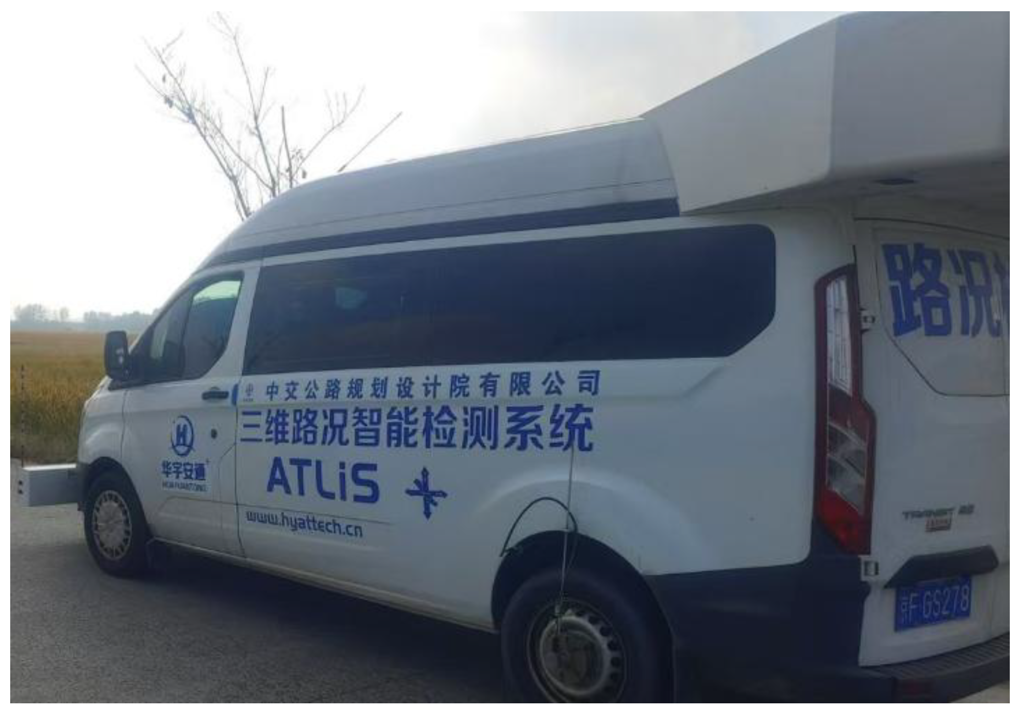
Figure 2.
Overall architecture of CGHN-Net.
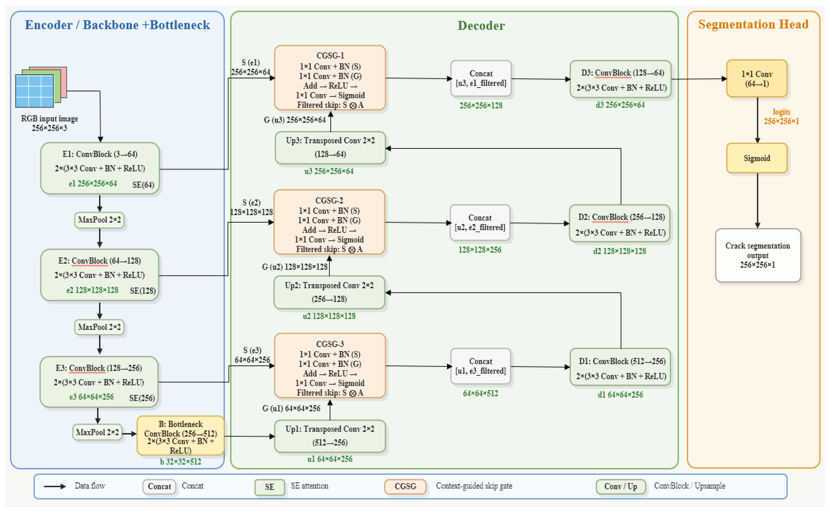
Figure 3.
Structure of the CGSG module.
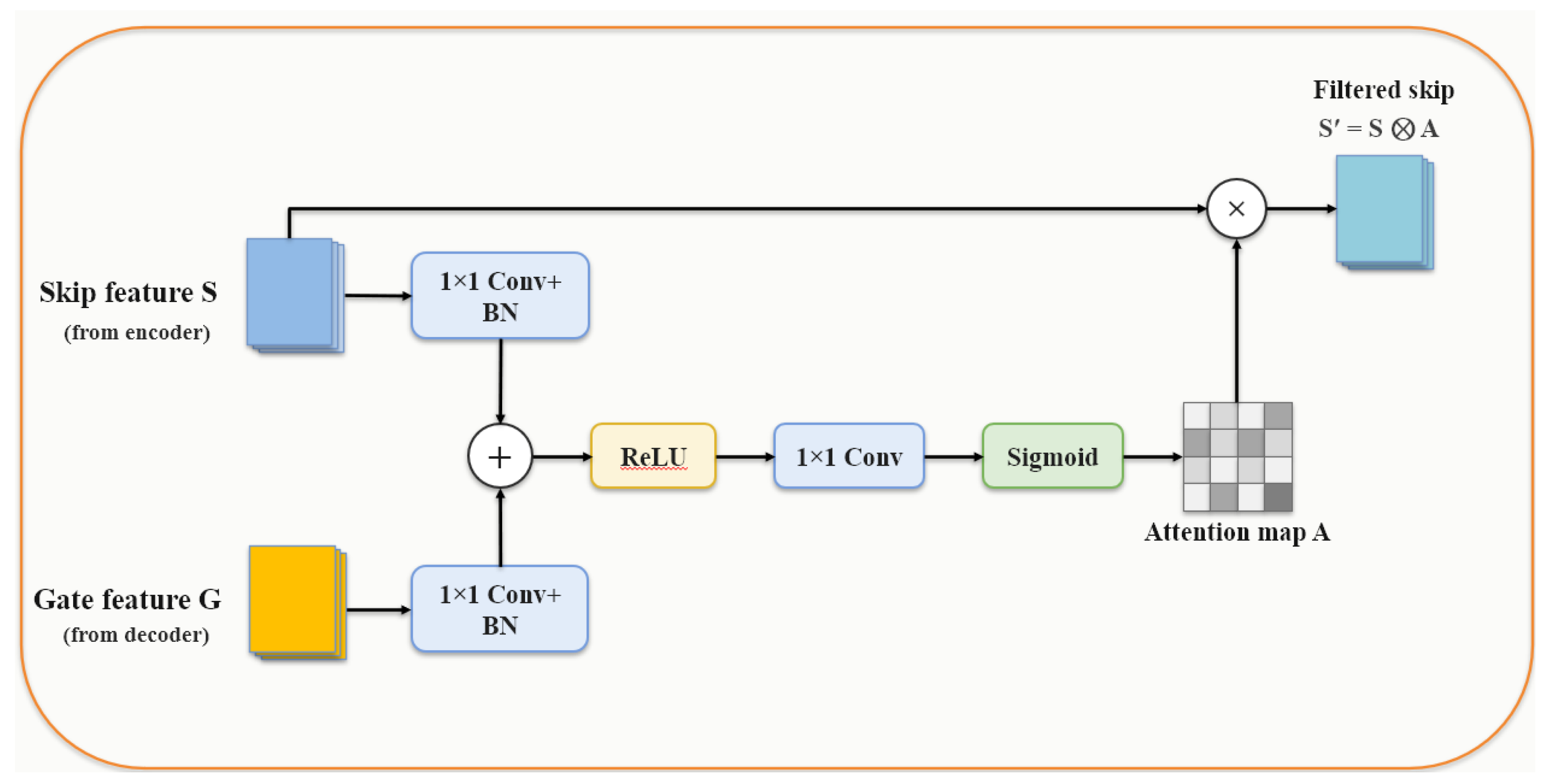
Figure 4.
Hard-negative background selection workflow for HNBS Loss.
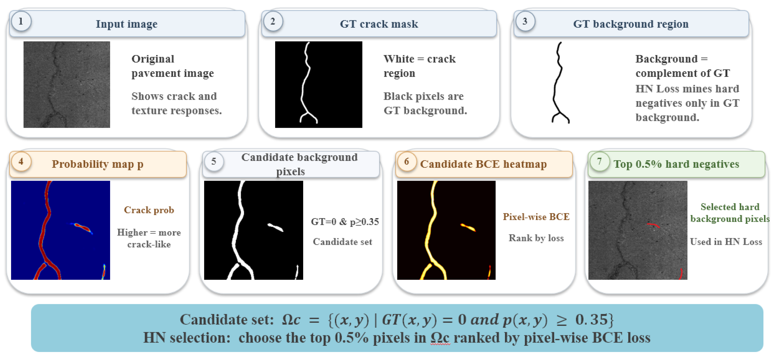
Figure 5.
Examples of pavement images and crack annotations.
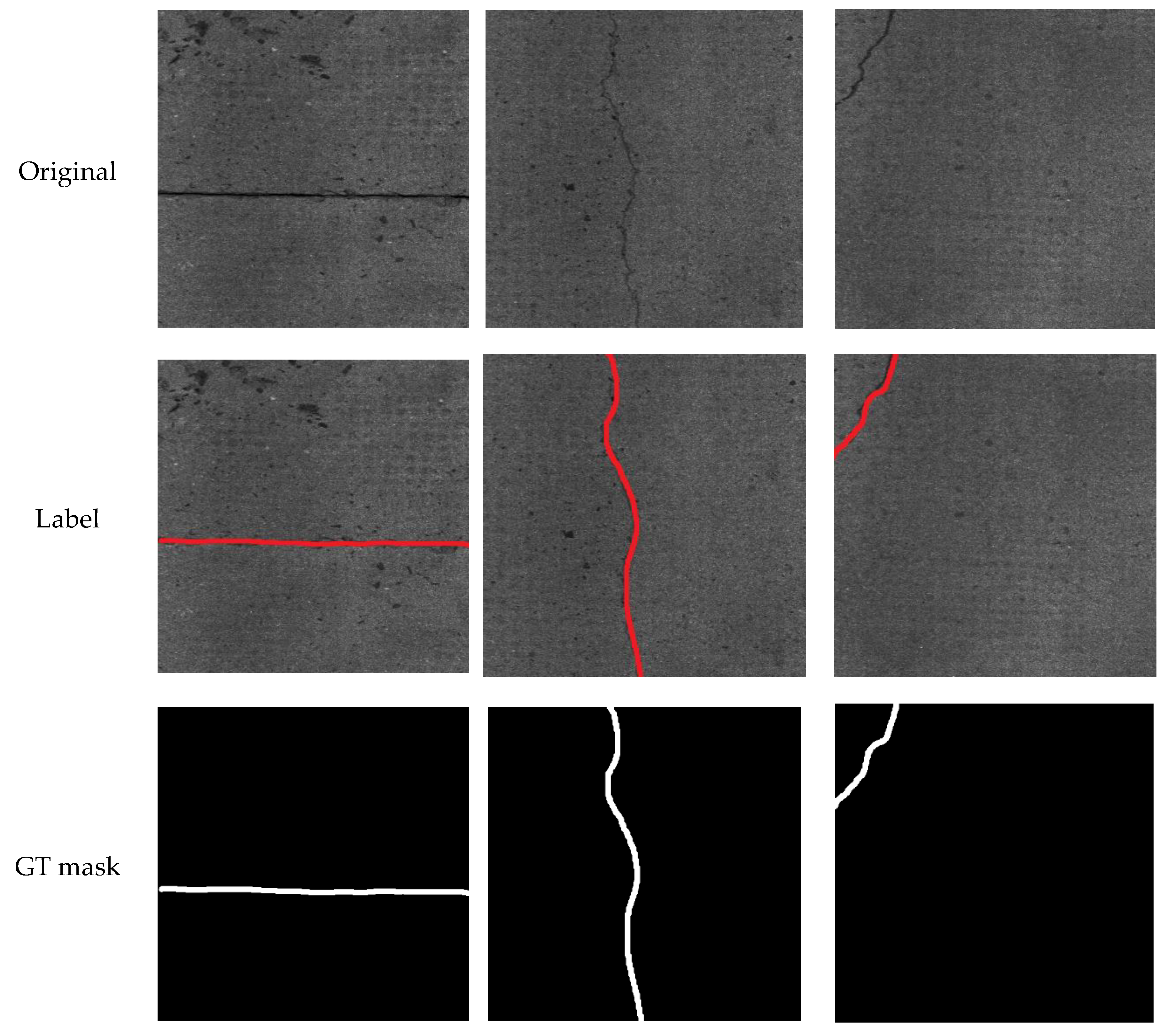
Figure 6.
Examples of data augmentation.
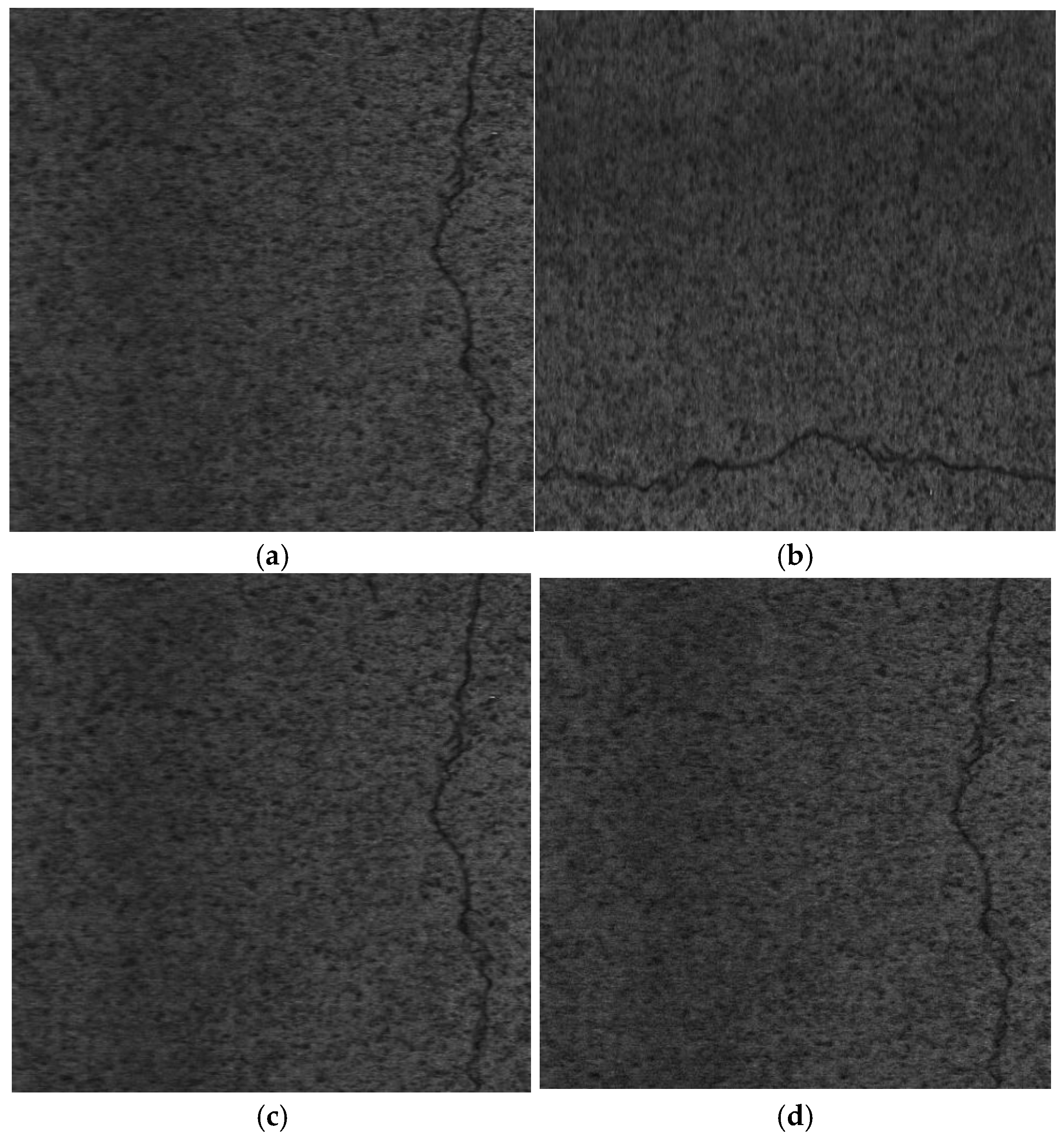
Figure 7.
Representative false-positive predictions on crack-free images from the held-out Road Section D subset.
Figure 7.
Representative false-positive predictions on crack-free images from the held-out Road Section D subset.
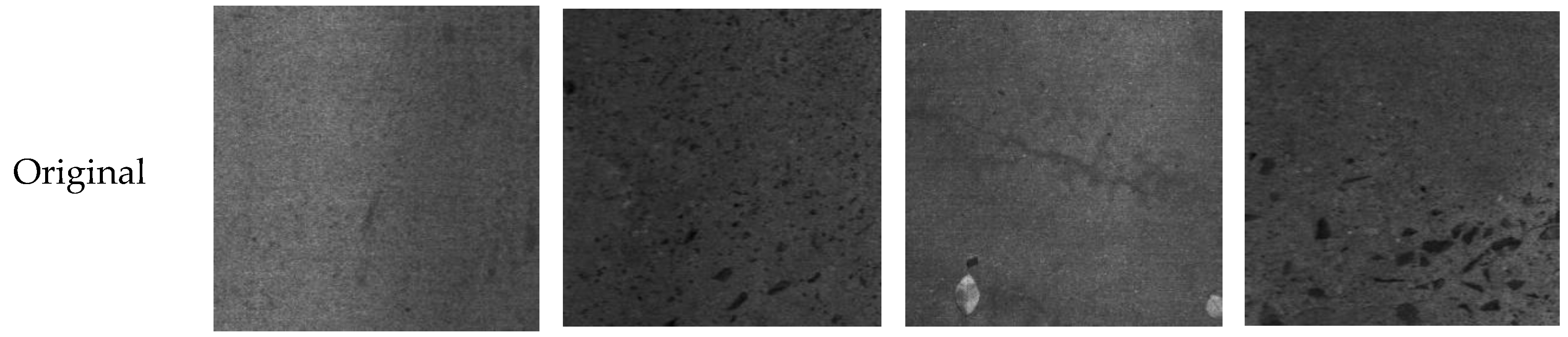
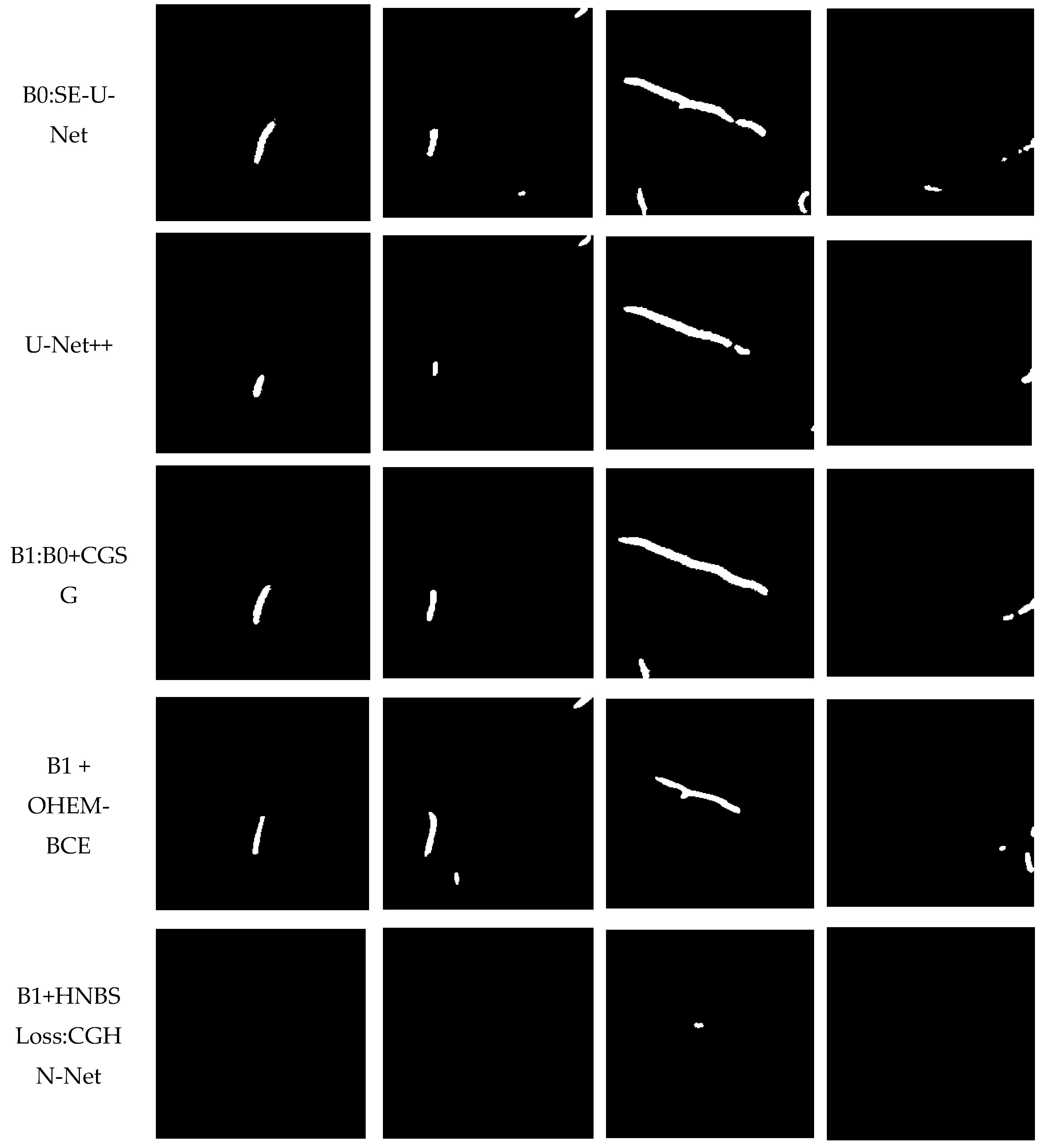
Figure 8.
Comparison of crack prediction results obtained by different models.
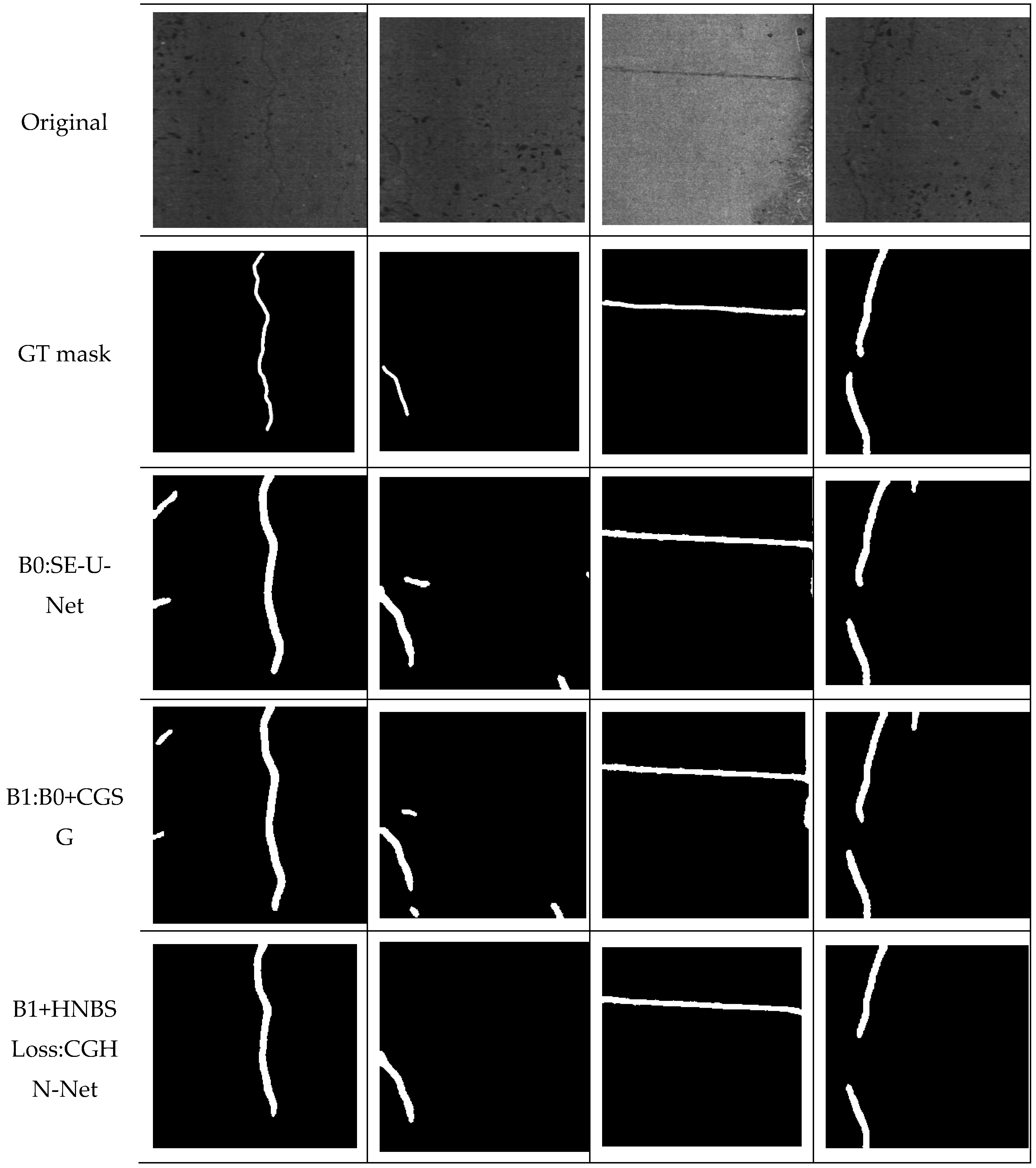
Figure 9.
Local comparison of texture-induced false-positive suppression.
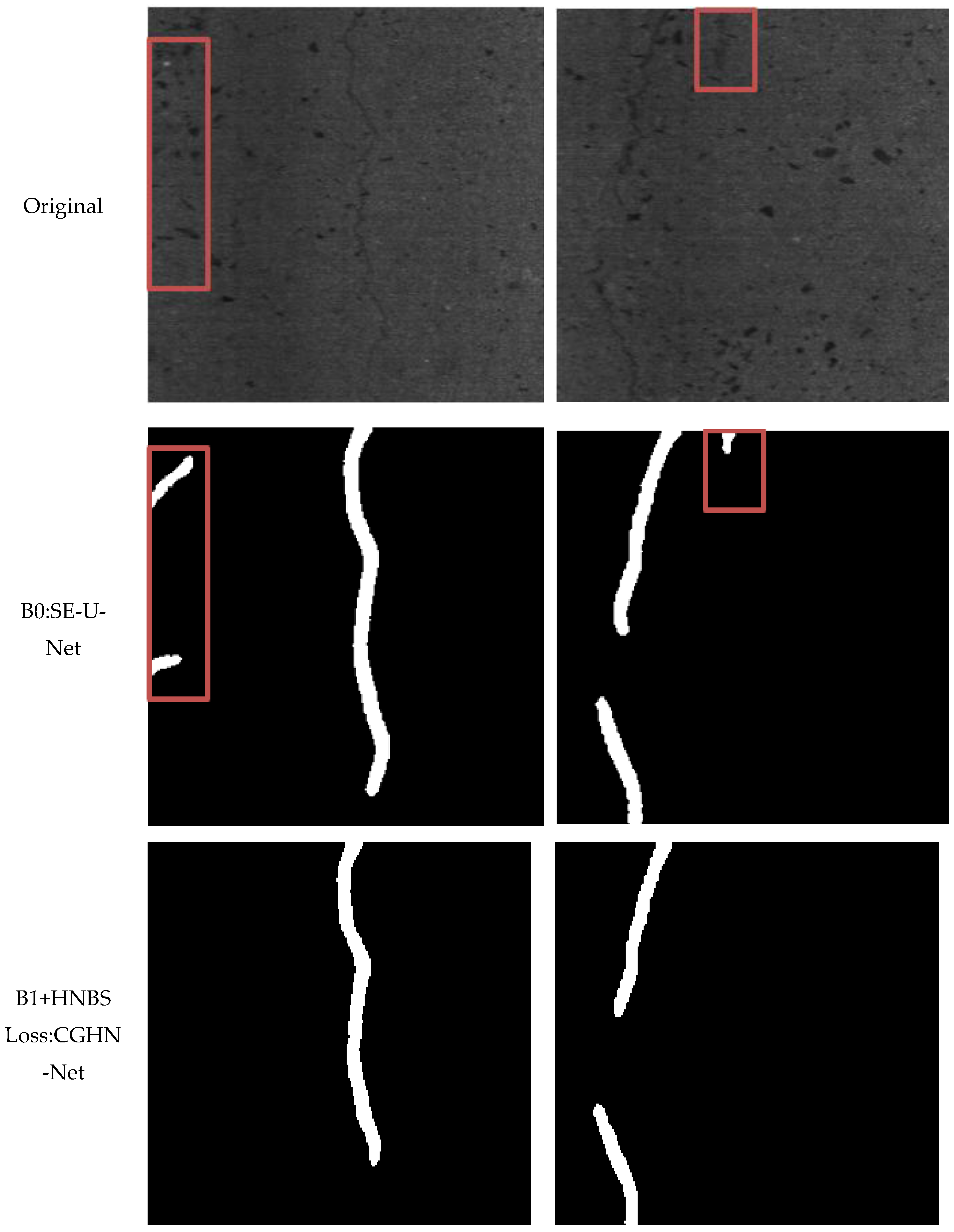

Table 1.
Main specifications of the vehicle-mounted sensing and image-acquisition system.
| Item | Configuration |
| Acquisition platform | Vehicle-mounted multifunctional pavement inspection system |
| Vehicle platform | Modified Ford Transit |
| Imaging sensor | Industrial-grade CCD camera |
| Additional sensors | Three-dimensional laser scanner, GPS, and IMU |
| Pavement measurement resolution | Approximately 1 mm |
| Image type used in this study | Two-dimensional grayscale pavement image |
| Original image size used in the dataset | 512 × 512 pixels |
| Network input size | 256 × 256 pixels |
| Operating speed | Approximately 5–30 km/h |
| Speed in crack-dense areas | Approximately 5–15 km/h |
| Sampling interval in crack-dense areas | Approximately 10 cm |
| Sampling interval on regular sections | Approximately 20 cm |
| Glare suppression | Polarizing filter |
| Exposure control | Dynamic exposure adjustment |
| Frame quality control | Frames with more than 30% occlusion were excluded or reacquired |
| Acquisition region | High-standard farmland field roads in Huzhou, China |
| Acquisition sessions | Three independent days |
| Dataset partition | Different acquisition days and mutually exclusive road sections |
Table 2.
Operation-by-operation comparison between the standard Attention Gate and CGSG.
| Comparison item | Standard Attention Gate | CGSG |
| Encoder input | High-resolution skip feature | High-resolution skip feature |
| Decoder input | Lower-resolution decoder feature | Already upsampled decoder feature |
| Encoder projection | 2 × 2, stride-2 Conv+BN | 1 × 1 Conv+BN |
| Decoder projection | 1 × 1 Conv+BN | 1 × 1 Conv+BN |
| Feature fusion | Element-wise addition | Element-wise addition |
| Nonlinearity | ReLU | ReLU |
| Attention generation | 1 × 1 Conv+Sigmoid | 1 × 1 Conv+Sigmoid |
| Internal skip downsampling | Required | Not required |
| Attention-map upsampling | Required | Not required |
| Output | Original skip weighted by attention map | Original skip weighted by attention map |
| Deployment | Three controlled skip gates | Three same-resolution skip gates |
| Primary objective | Generic spatial selection | Texture suppression with weak-crack preservation |
Table 3.
Controlled segmentation comparison of B0, the standard Attention Gate, and CGSG.
| Model | Dice | IoU | Precision | Recall | FP Area Ratio |
| B0: SE-U-Net | 0.8624 ± 0.0063 | 0.7708 ± 0.0105 | 0.8624 ± 0.0189 | 0.8796 ± 0.0280 | 0.0049 ± 0.0007 |
| SE-U-Net + Standard AG | 0.8403 ± 0.0058 | 0.7357 ± 0.0085 | 0.8785 ± 0.0164 | 0.8212 ± 0.0149 | 0.0040 ± 0.0008 |
| B1: SE-U-Net + CGSG | 0.8643 ± 0.0021 | 0.7717 ± 0.0047 | 0.8670 ± 0.0125 | 0.8769 ± 0.0172 | 0.0047 ± 0.0005 |
Table 4.
Model complexity and inference speed of the controlled variants.
| Model | Params (M) | GFLOPs | Time (ms/image) | FPS |
| B0: SE-U-Net | 7.7114 | 36.8270 | 12.6682 ± 0.6023 | 78.94 |
| SE-U-Net + Standard AG | 7.9706 | 37.4360 | 13.9419 ± 0.2864 | 71.73 |
| B1: SE-U-Net + CGSG | 7.8121 | 37.6507 | 13.7077 ± 0.2623 | 72.95 |
Table 5.
Controlled comparison of HNBS Loss and global pixel-wise OHEM-BCE under the B1 architecture.
Table 5.
Controlled comparison of HNBS Loss and global pixel-wise OHEM-BCE under the B1 architecture.
| Model / loss | Dice | IoU | Precision | Recall | FP Area Ratio |
| B1: SE-U-Net + CGSG | 0.8643 ± 0.0021 | 0.7717 ± 0.0047 | 0.8670 ± 0.0125 | 0.8769 ± 0.0172 | 0.0047 ± 0.0005 |
| B1 + OHEM-BCE | 0.8453 ± 0.0067 | 0.7442 ± 0.0114 | 0.8522 ± 0.0137 | 0.8553 ± 0.0210 | 0.0053 ± 0.0008 |
| B1 + HNBS Loss | 0.8682 ± 0.0055 | 0.7791 ± 0.0102 | 0.8780 ± 0.0161 | 0.8734 ± 0.0266 | 0.0042 ± 0.0008 |
Table 6.
Twenty-epoch validation results for the sensitivity analysis of HNBS hyperparameters under random seed 2026.
Table 6.
Twenty-epoch validation results for the sensitivity analysis of HNBS hyperparameters under random seed 2026.
| Config | τ | ρ | λ_HNBS | Dice | IoU | Precision | Recall | FP Area Ratio |
| S2 | 0.35 | 0.0050 | 0.010 | 0.5061 | 0.3498 | 0.4389 | 0.7388 | 0.0059 |
| S3 | 0.45 | 0.0050 | 0.010 | 0.4902 | 0.3409 | 0.4388 | 0.6607 | 0.0064 |
| S5 | 0.35 | 0.0100 | 0.010 | 0.4890 | 0.3391 | 0.4356 | 0.6635 | 0.0061 |
| S1 | 0.25 | 0.0050 | 0.010 | 0.4878 | 0.3358 | 0.4175 | 0.7019 | 0.0068 |
| S6 | 0.35 | 0.0050 | 0.005 | 0.4668 | 0.3194 | 0.3808 | 0.6953 | 0.0072 |
| S4 | 0.35 | 0.0025 | 0.010 | 0.4660 | 0.3177 | 0.4013 | 0.6854 | 0.0070 |
| S7 | 0.35 | 0.0050 | 0.020 | 0.3804 | 0.2631 | 0.3272 | 0.5373 | 0.0081 |
Table 7.
Experimental environment.
| Item | Configuration |
| Operating System | Windows-11-10.0.22631-SP0 |
| Python | 3.12.0 |
| PyTorch / Torchvision | 2.2.0+cu118 / 0.17.0+cu118 |
| CUDA / cuDNN | CUDA 11.8 / cuDNN 8700 |
| GPU | NVIDIA GeForce RTX 4060 Ti, 8.0 GB |
| CPU | Intel64 Family 6 Model 151 Stepping 2, GenuineIntel |
| OpenCV / NumPy / Pandas / Pillow | OpenCV 4.13.0; NumPy 1.26.4; Pandas 2.2.3; Pillow 11.1.0 |
Table 8.
Test-set crack segmentation performance under three random seeds.
| Model | seed | Dice | IoU | Precision | Recall | FP Area Ratio |
| U-Net | 2026 | 0.8539 | 0.7554 | 0.8693 | 0.8556 | 0.0047 |
| U-Net | 2025 | 0.8623 | 0.7679 | 0.8514 | 0.8880 | 0.0056 |
| U-Net | 42 | 0.8546 | 0.7587 | 0.8536 | 0.8737 | 0.0056 |
| Attention U-Net | 2026 | 0.8564 | 0.7599 | 0.8757 | 0.8533 | 0.0045 |
| Attention U-Net | 2025 | 0.8484 | 0.7474 | 0.8573 | 0.8545 | 0.0052 |
| Attention U-Net | 42 | 0.8652 | 0.7761 | 0.8564 | 0.8914 | 0.0055 |
| UNet++ | 2026 | 0.8656 | 0.7746 | 0.8667 | 0.8795 | 0.0048 |
| UNet++ | 2025 | 0.8466 | 0.7452 | 0.8729 | 0.8353 | 0.0045 |
| UNet++ | 42 | 0.8649 | 0.7752 | 0.8652 | 0.8803 | 0.0049 |
| DeepLabV3+ | 2026 | 0.8357 | 0.7261 | 0.8588 | 0.8303 | 0.0049 |
| DeepLabV3+ | 2025 | 0.8286 | 0.7165 | 0.8449 | 0.8347 | 0.0055 |
| DeepLabV3+ | 42 | 0.8424 | 0.7380 | 0.8489 | 0.8539 | 0.0056 |
| SegFormer-B0 | 2026 | 0.7708 | 0.6438 | 0.7883 | 0.7759 | 0.0074 |
| SegFormer-B0 | 2025 | 0.7611 | 0.6307 | 0.7881 | 0.7561 | 0.0069 |
| SegFormer-B0 | 42 | 0.7639 | 0.6323 | 0.8024 | 0.7528 | 0.0063 |
| CGHN-Net | 2026 | 0.8710 | 0.7834 | 0.8791 | 0.8761 | 0.0041 |
| CGHN-Net | 2025 | 0.8719 | 0.7866 | 0.8615 | 0.8988 | 0.0052 |
| CGHN-Net | 42 | 0.8618 | 0.7676 | 0.8938 | 0.8457 | 0.0034 |
Table 9.
Test-set crack segmentation performance of different models (mean ± standard deviation).
| Model | Dice | IoU | Precision | Recall | FP Area Ratio |
| U-Net | 0.8568 ± 0.0047 | 0.7605 ± 0.0064 | 0.8580 ± 0.0098 | 0.8723 ± 0.0162 | 0.0053 ± 0.0005 |
| Attention U-Net | 0.8566 ± 0.0084 | 0.7611 ± 0.0143 | 0.8630 ± 0.0109 | 0.8663 ± 0.0216 | 0.0050 ± 0.0005 |
| UNet++ | 0.8590 ± 0.0107 | 0.7649 ± 0.0170 | 0.8682 ± 0.0041 | 0.8650 ± 0.0258 | 0.0047 ± 0.0002 |
| DeepLabV3+ | 0.8355 ± 0.0069 | 0.7268 ± 0.0107 | 0.8508 ± 0.0071 | 0.8395 ± 0.0125 | 0.0053 ± 0.0003 |
| SegFormer-B0 | 0.7653 ± 0.0050 | 0.6356 ± 0.0071 | 0.7929 ± 0.0082 | 0.7616 ± 0.0125 | 0.0068 ± 0.0005 |
| CGHN-Net | 0.8682 ± 0.0055 | 0.7791 ± 0.0102 | 0.8780 ± 0.0161 | 0.8734 ± 0.0266 | 0.0042 ± 0.0008 |
Table 10.
Model complexity, peak GPU memory, and inference speed of the representative segmentation models.
Table 10.
Model complexity, peak GPU memory, and inference speed of the representative segmentation models.
| Model | Params (M) | GFLOPs | Peak GPU memory (MB) | Time (ms/image) | FPS |
| U-Net | 7.7002 | 36.8197 | 152.94 | 5.6853 ± 0.1451 | 175.89 |
| Attention U-Net | 7.7873 | 37.6434 | 237.25 | 6.4305 ± 0.0983 | 155.51 |
| UNet++ | 8.8196 | 69.8792 | 261.50 | 12.2416 ± 0.0013 | 81.69 |
| DeepLabV3+ | 5.9269 | 10.1004 | 158.67 | 1.8506 ± 0.0315 | 540.38 |
| SegFormer-B0 | 3.7144 | 1.7726 | 188.55 | 4.8280 ± 0.0896 | 207.12 |
| CGHN-Net | 7.8121 | 37.6507 | 274.60 | 6.8320 ± 0.0089 | 146.37 |
Table 11.
Paired per-image statistical comparison between CGHN-Net and UNet++ over the same 87 test images.
Table 11.
Paired per-image statistical comparison between CGHN-Net and UNet++ over the same 87 test images.
| Metric | Mean paired difference | 95% bootstrap CI | Raw p | Holm-adjusted p | Win rate (%) |
| Dice | 0.0102 | [0.0059, 0.0149] | <0.0001 | 0.0001 | 67.8 |
| IoU | 0.0154 | [0.0089, 0.0222] | <0.0001 | <0.0001 | 69.0 |
| Precision | 0.0105 | [0.0041, 0.0171] | 0.0020 | 0.0040 | 58.6 |
| Recall | 0.0092 | [0.0033, 0.0152] | 0.0040 | 0.0040 | 64.4 |
| FP Area Ratio reduction |
0.00055 | [0.00023, 0.00090] | 0.0013 | 0.0038 | 56.3 |
Table 12.
Comparison of raw and post-processed segmentation results for UNet++ and CGHN-Net.
| Model | Evaluation output | Dice | IoU | Precision | Recall | FP Area Ratio |
| UNet++ | Raw thresholded output | 0.8540 ± 0.0116 | 0.7565 ± 0.0183 | 0.8666 ± 0.0022 | 0.8661 ± 0.0242 | 0.0049 ± 0.0001 |
| UNet++ | Post-processed output | 0.8590 ± 0.0107 | 0.7649 ± 0.0170 | 0.8682 ± 0.0041 | 0.8650 ± 0.0258 | 0.0047 ± 0.0002 |
| CGHN-Net | Raw thresholded output | 0.8650 ± 0.0046 | 0.7732 ± 0.0088 | 0.8790 ± 0.0169 | 0.8752 ± 0.0243 | 0.0042 ± 0.0009 |
| CGHN-Net | Post-processed output | 0.8682 ± 0.0055 | 0.7791 ± 0.0102 | 0.8780 ± 0.0161 | 0.8734 ± 0.0266 | 0.0042 ± 0.0008 |
Table 13.
False-positive evaluation on the held-out crack-free subset from Road Section D.
| Model | Raw image-level FAR | Post image-level FAR | Raw FP Area Ratio | Post FP Area Ratio |
| B0:SE-U-Net | 0.3700 ± 0.0556 | 0. 3100 ± 0.0529 | 0.0037 ± 0.0010 | 0.0035 ± 0.0009 |
| U-Net++ | 0.2400 ± 0.0264 | 0.1766 ± 0.0351 | 0.0023 ± 0.0002 | 0.0021 ± 0.0002 |
| B1:B0+CGSG | 0.4166 ± 0.0808 | 0.3100 ± 0.0556 | 0.0040 ± 0.0008 | 0.0037 ± 0.0007 |
| B1 + OHEM-BCE | 0.3330 ± 0.0115 | 0.2833 ± 0.0288 | 0.0042 ± 0.0008 | 0.0039 ± 0.0007 |
| B1+HNBS Loss:CGHN-Net | 0.1866 ± 0.0723 | 0.1300 ± 0.0335 | 0.0019 ± 0.0006 | 0.0018 ± 0.0006 |
Table 14.
Ablation experiment results for CGSG and HNBS Loss (three random seeds).
| Model | CGSG | HNBS Loss | Seed | Dice | IoU | Precision | Recall | FP Area Ratio |
| B0:SE-U-Net | × | × | 2026 | 0.8647 | 0.7743 | 0.8408 | 0.9075 | 0.0057 |
| B0:SE-U-Net | × | × | 2025 | 0.8672 | 0.7791 | 0.8706 | 0.8796 | 0.0046 |
| B0:SE-U-Net | × | × | 42 | 0.8553 | 0.759 | 0.8759 | 0.8516 | 0.0044 |
| B0+HNBS Loss | × | √ | 2026 | 0.8522 | 0.7552 | 0.8618 | 0.8605 | 0.0048 |
| B0+HNBS Loss | × | √ | 2025 | 0.8561 | 0.7605 | 0.8667 | 0.8610 | 0.0048 |
| B0+HNBS Loss | × | √ | 42 | 0.8495 | 0.7483 | 0.8884 | 0.8279 | 0.0038 |
| B1:B0+CGSG | √ | × | 2026 | 0.8649 | 0.7731 | 0.8571 | 0.8889 | 0.0050 |
| B1:B0+CGSG | √ | × | 2025 | 0.8619 | 0.7665 | 0.8811 | 0.8572 | 0.0041 |
| B1:B0+CGSG | √ | × | 42 | 0.8660 | 0.7755 | 0.8628 | 0.8846 | 0.0050 |
| B1+HNBS Loss:CGHN-Net | √ | √ | 2026 | 0.8710 | 0.7834 | 0.8791 | 0.8761 | 0.0041 |
| B1+HNBS Loss:CGHN-Net | √ | √ | 2025 | 0.8719 | 0.7866 | 0.8615 | 0.8988 | 0.0052 |
| B1+HNBS Loss:CGHN-Net | √ | √ | 42 | 0.8618 | 0.7676 | 0.8938 | 0.8457 | 0.0034 |
Table 15.
Ablation experiment results for CGSG and HNBS Loss (mean ± standard deviation).
| Model | CGSG | HNBS Loss | Dice | IoU | Precision | Recall | FP Area Ratio |
| B0:SE-U-Net | × | × | 0.8624±0.0063 | 0.7708±0.0105 | 0.8624±0.0189 | 0.8796±0.0280 | 0.0049±0.0007 |
| B0+HNBS Loss | × | √ | 0.8526±0.0033 | 0.7547±0.0061 | 0.8723±0.0141 | 0.8498±0.0189 | 0.0045±0.0005 |
| B1:B0+CGSG | √ | × | 0.8643±0.0021 | 0.7717±0.0047 | 0.8670±0.0125 | 0.8769±0.0172 | 0.0047±0.0005 |
| B1+HNBS Loss:CGHN-Net | √ | √ | 0.8682±0.0055 | 0.7791±0.0102 | 0.8780±0.0161 | 0.8734±0.0266 | 0.0042±0.0008 |
Disclaimer/Publisher’s Note: The statements, opinions and data contained in all publications are solely those of the individual author(s) and contributor(s) and not of MDPI and/or the editor(s). MDPI and/or the editor(s) disclaim responsibility for any injury to people or property resulting from any ideas, methods, instructions or products referred to in the content. |
© 2026 by the authors. Licensee MDPI, Basel, Switzerland. This article is an open access article distributed under the terms and conditions of the Creative Commons Attribution (CC BY) license (http://creativecommons.org/licenses/by/4.0/).
Copyright: This open access article is published under a Creative Commons CC BY 4.0 license, which permit the free download, distribution, and reuse, provided that the author and preprint are cited in any reuse.