

Submitted:
08 July 2026
Posted:
21 July 2026
You are already at the latest version
Abstract
Rotating traversable wormholes provide a horizonless setting in which to investigate wave dynamics beyond the separable structures familiar from black-hole perturbation theory. We study scalar perturbations in the rotating AdS-Teo wormhole and show that the absence of separability naturally leads to a coupled-channel formulation in which the angular harmonic modes interact through a matrix-valued Sturm-Liouville operator. Imposing regularity at the wormhole throat together with asymptotically anti-de Sitter boundary conditions yields a determinant quantization condition that determines a discrete normal-mode spectrum. A controlled two-channel truncation illustrates how angular-channel mixing produces frequency shifts, spectral repulsion, and collective mode reorganization. From the asymptotic solutions, we construct a matrix-valued boundary response function whose poles coincide with the bulk normal-mode frequencies, while its off-diagonal components provide a direct signature of rotation-induced channel mixing. We further investigate the renormalized vacuum polarization, whose interference terms reveal local quantum signatures of non-separability, and examine semiclassical geodesic correlators as complementary probes of two-boundary connectivity. These results suggest that coupled-channel spectral theory provides a natural organizing principle for rotating, non-separable geometries, replacing conventional mode separability with a framework based on collective normal modes, matrix-valued response functions, and coupled quantum observables.
Keywords:
rotating wormholes
; anti-de sitter spacetime
; scalar perturbations
; coupled-channel spectral theory
; matrix sturm-liouville operators
; normal modes
; holographic response
; vacuum polarization
; mode coupling
; spectral theory
1. Introduction
Quantum field theory in curved spacetime provides a framework for understanding how geometry, symmetry, and boundary conditions shape the dynamics of quantum fields in gravitational backgrounds [1,2,3,4,5,6]. A central lesson is that physical observables, including particle content, spectra, response functions, and local vacuum polarization, depend not only on local geometry, but also on global structure and asymptotic boundary conditions.
Black-hole spacetimes provide a paradigmatic example. Event horizons lead to dissipative dynamics and phenomena such as Hawking radiation [4]. At the level of wave propagation, these features are reflected in quasinormal-mode spectra and in the analytic structure of retarded Green’s functions [7]. A defining property of rotating black holes is the separability of the wave equation. In Kerr spacetime, the Teukolsky admits a complete separation of variables [8], a consequence of hidden geometric structure associated with a rank-two Killing tensor and the Carter constant [9,10]. This separability underlies much of blackhole perturbation theory and has also played a central role in the identification of hidden conformal structures in rotating spacetimes [11,12].
These developments raise a broader question: to what extent are such spectral and holographic structures tied to separability and horizons, and to what extent do they arise more generally from geometry and boundary conditions? Most analyses of rotating spacetimes rely heavily on separability, and comparatively little is known about wave dynamics in rotating, horizonless geometries where separability fails.
This naturally raises a more fundamental question. Much of black-hole perturbation theory relies on separability, which reduces the wave equation to independent radial problems. If separability is absent, what replaces it as the organizing principle for wave dynamics and spectral structure? The central goal of this work is to address this question in the context of a rotating, horizonless AdS wormhole and to show that the resulting dynamics are most naturally formulated in terms of coupled-channel spectral theory. Rather than decomposing into independent angular sectors, the scalar field organizes into interacting channels whose collective behavior determines the physical spectrum and associated boundary observables.
Traversable wormholes provide a natural setting in which to explore this question. These geometries connect multiple asymptotic regions through a smooth throat and are supported by nontrivial matter configurations [13,14]. Rotating wormhole solutions, such as the Teo geometry [15], incorporate frame dragging and can exhibit phenomena analogous to those of rotating black-holes while remaining entirely horizonless.
In this work, we study scalar perturbations in a rotating AdS-Teo wormhole background. Embedding the geometry in asymptotically AdS spacetime provides a well-defined global spectral problem together with a natural setting for boundary observables and holographic response functions.
A central feature of the rotating AdS-Teo geometry is that the scalar wave equation is not generically separable. Unlike Kerr spacetime, where hidden symmetry structures associated with the Carter constant permit complete separation of the wave equation [9,10], the rotating AdS-Teo wormhole does not generically admit such a separable decomposition in the formulation considered here. The scalar dynamics therefore naturally organize into a coupled-channel system in which different angular sectors interact through the geometry.
The distinction is fundamentally geometric. In Kerr spacetime, separability is possible because the hidden symmetry generated by the rank-two Killing tensor provides an additional conserved quantity beyond the energy and axial angular momentum. This additional structure renders the geodesic and wave dynamics completely integrable and permits the decomposition of the scalar field into independent radial and angular sectors. In the rotating AdS-Teo geometry considered here, no analogous hidden symmetry structure is known generically, and the scalar dynamics therefore organize naturally into interacting angular channels rather than into fully separated mode equations.
Expanding the field in angular harmonics leads not to a single radial equation, but to a matrix-valued coupled-channel system. The spectral problem therefore becomes a matrix-valued Sturm-Liouville problem rather than a standard single-channel eigenvalue problem [16,17,18,19]. In this sense, the analysis is based not on integrable mode separation, but on the spectral theory of coupled operators.
This coupled structure reorganizes the spectral analysis. Instead of imposing normalizability on a single radial mode, one must construct a basis of solutions regular at the throat and determine whether a nontrivial linear combination satisfies the AdS boundary conditions. The resulting quantization condition takes the determinant form
which generalizes the familiar scalar condition . The physical spectrum is therefore a collective phenomenon arising from interaction between angular channels, analogous to coupled-mode reorganization phenomena encountered in multichannel scattering and spectral theory [16,17].
Despite the coupled-channel language and the close analogy with multichannel scattering theory, this problem is fundamentally a confined spectral problem rather than an asymptotic scattering problem. The reflecting AdS boundary conditions discretize the spectrum and lead to globally supported normal modes analogous to bound states in a self-adjoint operator system. The resulting poles therefore remain on the real frequency axis and describe stable collective oscillations of the coupled wormhole geometry rather than dissipative scattering resonances.
To make this structure explicit, we analyze a controlled two-channel truncation of the coupled system, following the standard strategy of finite-channel reduction commonly used in coupled-mode and multichannel spectral problems [16,17]. This provides a concrete illustration of how angular-channel mixing shifts the normal-mode frequencies, produces spectral repulsion, and reorganizes the collective spectral structure. In the rotating wormhole geometry, rotation does not merely produce a local frequency shift of the form ; rather, it induces coupling between different angular sectors. This angular-mode mixing is one of the defining dynamical features of the system. Such coupled-channel dynamics are familiar in multicomponent wave and scattering systems, where the physical spectrum is determined by the collective behavior of interacting sectors rather than by isolated single-mode evolution [16,17].
At the level of boundary observables, the asymptotic behavior of the bulk field defines the matrix-valued response function , whose poles coincide with the bulk normal-mode frequencies. The off-diagonal components encode angular-channel mixing and provide a direct boundary signature of the non-separable geometry. Because the wormhole spacetime is smooth and horizonless, the spectral problem is conservative and self-adjoint, and the poles correspond to normal modes rather than dissipative quasinormal modes. In this sense, the response structure is closer to a coupled normal-mode system than to the quasinormal spectra characteristic of black-hole geometries. The resulting matrix Green’s functions are closely related to multichannel response systems and to holographic models with operator mixing [20,21,22], although we do not assume a specific dual field-theoretic interpretation.
Near the throat, we identify a local conformal-type organization of the radial differential operator. Unlike hidden conformal structures in black-hole physics, which are closely associated with horizons, this structure arises at a regular interior point and acts on a vector of coupled modes. It therefore organizes the local solution space without determining the global spectrum. The physical spectrum is instead fixed only after the globally regular throat solutions are matched to the asymptotic AdS boundary conditions of the full coupled operator problem.
We also analyze local quantum observables through the renormalized vacuum polarization . In the coupled-channel formulation, the resulting Wightman function contains interference terms between angular channels. These interference terms provide a local quantum signature of non-separability and distinguish the rotating wormhole from both spherically symmetric wormholes and fully separable black-hole backgrounds.
Finally, we complement the wave-based analysis with a semiclassical geodesic probe of two-boundary connectivity. In the large conformal dimension limit, cross-boundary correlators are controlled by renormalized spacelike geodesic lengths through the wormhole interior. This provides a geometric diagnostic of traversability complementary to the spectral and Green’s function analysis.
The goal of this work is therefore not merely to analyze a particular wormhole solution, but to investigate what replaces separability as the organizing principle for wave dynamics in rotating, non-separable, horizonless geometries. We argue that coupled-channel spectral theory provides the appropriate framework, in which angular harmonics become interacting spectral channels, normal modes emerge collectively from coupled operators, and boundary response functions acquire an intrinsically matrix-valued structure. This unified perspective connects global spectral theory, holographic response, near-throat operator organization, and local quantum observables within a single description of wave dynamics in rotating wormhole geometries.
The paper is organized as follows. In Sec. 2, we introduce the rotating AdS-Teo wormhole geometry, construct the proper-distance formulation, and derive the coupled scalar-field equations. In Sec. 3, we analyze the near-throat structure of the coupled system and identify its local conformal-type organization. In Sec. 4, we formulate the global coupled spectral problem, construct the asymptotic AdS solution space, and derive the determinant quantization condition. In Sec. 5, we investigate channel mixing through a controlled two-channel truncation and develop the associated matrix-valued holographic response framework. In Sec. 6, we construct boundary observables and analyze their spectral signatures. In Sec. 7, we study local quantum observables through the renormalized vacuum polarization and identify interference effects arising from angular-channel mixing. Finally, in Sec. 8, we summarize the results and discuss the broader implications of coupled-channel spectral theory as an organizing framework for wave dynamics in rotating, non-separable geometries.
2. Geometry and Scalar Field Setup
2.1. Rotating AdS-Teo Geometry and Global Structure
We begin with the rotating Teo wormhole spacetime [15]. In its stationary and axisymmetric form, the metric may be written as
Here is the redshift function, is the shape function, controls the angular deformation of the two-spheres, and is the frame-dragging angular velocity. The wormhole throat is located at , where
For a traversable wormhole, the throat must satisfy the flare-out condition
which ensures that the spatial geometry opens outward rather than pinching off [13,14]. In the original construction of Teo [15], a simple and widely used choice of metric functions is
For this choice of shape function, , one finds
Thus the flare-out condition is satisfied, confirming that the spatial geometry opens outward at the throat and represents a smooth traversable wormhole.
These choices describe a rotating, asymptotically flat wormhole with rotation parameter a and throat scale . In particular, the frame-dragging term decays as , while ensures asymptotic flatness [13,14,15].
The reference global metric is
where L is the AdS curvature radius.
In this work, we consider an asymptotically AdS deformation of this geometry. In asymptotically flat spacetimes, scalar perturbations are naturally formulated as scattering problems with continuous frequency spectra and boundary conditions imposed at null infinity. While suitable for transmission and reflection problems, this structure does not lead naturally to a discrete spectral problem [10,23].
By contrast, asymptotically AdS geometries possess timelike conformal boundaries on which one may impose normalizability or reflective boundary conditions. This leads to a well-posed spectral problem with a discrete set of normal modes [24,25,26], since the reflective AdS boundaries admit only specific frequencies compatible with global normalizability conditions. The timelike AdS boundary also provides a natural setting for boundary observables and response functions.
We impose asymptotic conditions such that, at large r, the wormhole geometry approaches global AdS:
Combining the Teo wormhole structure with these AdS asymptotics, we adopt the stationary axisymmetric ansatz
The metric functions reduce to the canonical Teo expressions near the throat,
the deformation decays at large radius, so that the geometry approaches global AdS asymptotically.
The AdS deformation is encoded primarily through the asymptotic behavior of the redshift function , whose leading term reproduces the global AdS time-time component. This preserves the regular wormhole throat structure while modifying the asymptotic geometry.
The analysis in this paper assumes that the metric functions interpolate smoothly between the canonical Teo geometry near the throat and the asymptotically AdS region while preserving at the throat. Consequently, the local throat geometry remains that of the regular Teo wormhole, whereas the AdS deformation modifies only the asymptotic structure required for the global spectral problem.
Throughout this work, the rotating AdS-Teo geometry is treated as a fixed background spacetime on which the scalar field propagates. Questions related to the full Einstein field equations, matter sources, and nonlinear backreaction are therefore beyond the scope of this analysis.
We assume that all metric functions are smooth and finite at the throat and that throughout the domain of interest. Since a Killing horizon forms where the norm of a timelike Killing vector becomes null [27,28], the condition excludes horizon formation and ensures that the geometry remains horizonless.
The spacetime is stationary and axisymmetric, but not spherically symmetric. Consequently, while the Killing directions t and permit Fourier decomposition in time and azimuthal angle, the remaining -dependence is not generically separable. The scalar-field equation therefore develops couplings between different angular harmonic sectors, leading to the coupled-channel structure studied below.
To make the global structure precise, it is useful to perform a conformal compactification. In the physical metric , the asymptotic regions lie at (equivalently ) and are not part of the manifold itself. Consequently, the physical spacetime is noncompact, with the two asymptotic regions located at infinite coordinate distance. Conformal compactification provides a convenient way to represent these asymptotic regions as finite boundary components while preserving the causal structure of the spacetime. Introducing the conformal factor
we define the rescaled metric
Using the asymptotic AdS form, valid in the limit ,
the conformally rescaled metric
becomes
up to subleading corrections that vanish asymptotically. The hypersurface therefore lies at finite coordinate location in the conformally rescaled geometry.
In this sense, the conformal compactification brings the asymptotic AdS boundary to a finite coordinate location and extends the spacetime to a conformally completed manifold. Although the physical spacetime remains noncompact, its conformal completion contains the boundary as a finite geometric component. This feature is central to the formulation of global boundary-value problems and underlies the discrete normal-mode spectrum characteristic of asymptotically AdS geometries [24,25,29,30].
Since the induced metric at is Lorentzian,
the conformal boundary is timelike, meaning that signals can reach and return from the boundary in finite global time. This is a characteristic feature of AdS asymptotics and is what allows one to formulate a boundary-value problem with normalizable modes.
The wormhole contains two asymptotic AdS regions corresponding to . After conformal compactification, these become two disconnected timelike boundary components, denoted and .
A key feature of the geometry is that the throat is a regular interior point rather than a horizon. In proper-distance coordinates, the radial sector takes the form
which is manifestly regular at . Radial null curves satisfy
which remains finite across the throat. Thus, both null and timelike causal curves can pass smoothly through the throat and connect the two asymptotic AdS regions.
Conformal compactification preserves causal structure, so the two boundaries remain causally connected after compactification. The role of the compactification is therefore not to modify causality, but to make the asymptotic regions accessible and to provide a natural setting for boundary conditions and observables.
In summary, the rotating AdS-Teo wormhole admits two timelike conformal boundaries connected through a smooth horizonless throat. This global structure provides the geometric foundation for the coupled normal-mode spectrum, matrix-valued boundary response functions, and holographic observables studied in the following sections.
2.2. Regular Throat Coordinate and Scalar Field Reduction
For the spectral problem it is useful to introduce a regular proper-distance coordinate ℓ adapted to the wormhole throat:
The two asymptotic regions correspond to and .
Although the full metric is not separable in , the line element along curves of fixed defines the proper radial distance. Along such curves, the metric reduces to
The proper radial coordinate is therefore defined by
The two signs correspond to the two asymptotic regions of the wormhole. Choosing the throat as the origin , one obtains
The coordinate ℓ therefore ranges from to , with negative and positive values describing the left and right exterior regions, respectively, connected through the throat. Unlike the areal radius r, which attains a minimum value at the throat, the proper-distance coordinate ℓ passes smoothly through the throat and provides a single coordinate chart covering both asymptotic regions.
For the Teo choice
one obtains
Integrating the proper-distance relation gives
Choosing the throat as the origin, at , the explicit solution
realizes the two asymptotic branches discussed above. The inverse relation, , allows the metric to be expressed entirely in terms of the proper-distance coordinate.
Near the throat, writing with , one finds
Unlike the black-hole tortoise coordinate , which develops a logarithmic divergence near a horizon where , the proper-distance coordinate ℓ remains finite because the wormhole throat is a regular interior point with .
Using the proper-distance coordinate
which covers both asymptotic regions and places the throat at , the metric becomes
where
The proper-distance coordinate naturally distinguishes the two asymptotic regions of the wormhole:
corresponds to the left exterior region,
corresponds to the right exterior region, and the throat is located at
For a reflection-symmetric wormhole, the two exterior regions are geometrically identical. This symmetry is represented by the discrete transformation
This transformation exchanges the momentum and winding sectors while leaving the spectrum invariant. Consequently, the metric functions are even under reflection:
This reflection symmetry allows scalar modes to be classified by parity in ℓ without assuming separability of the scalar-field equation.
We now consider a minimally coupled scalar field of mass obeying
where
Because the spacetime is stationary and axisymmetric, the coordinates t and are Killing directions. We therefore decompose the field as
This uses only the exact symmetries generated by and .
One should not, however, assume a further factorization
unless the geometry possesses the additional structure required for separability. Such separability is special in Kerr spacetime, where the scalar wave equation and the Teukolsky equation separate due to a hidden symmetry associated with a rank-two Killing tensor [8,9]. This structure leads to the Carter constant and permits a complete decomposition into radial and angular sectors. In generic axisymmetric spacetimes lacking such a Killing tensor, one instead obtains coupled systems after projection onto an angular harmonic basis (consisting of spherical harmonics labeled by angular quantum numbers ), analogous to coupled-channel formulations familiar in scattering theory [17]. In such formulations, each angular harmonic sector acts as an individual propagation channel, while the off-diagonal couplings generated by the geometry mix the different channels dynamically.
The metric determinant is
Substituting the ansatz (36) into the Klein-Gordon equation yields
This is the full axisymmetric scalar-field equation for the rotating wormhole background.
The combination arises directly from the mixed t- structure of the metric. Substituting into the kinetic term yields
The quantity
is therefore the local co-rotating frequency, namely the frequency measured in a frame locally rotating with angular velocity . Because may depend on both ℓ and , it generically contributes to angular-radial mode coupling.
In separable rotating geometries, such as Kerr or BTZ, the combination typically appears as a shifted co-rotating frequency within an otherwise independent radial equation [8,32]. The angular quantum numbers remain good labels, and rotation modifies the spectrum primarily through frequency shifts and superradiant structure.
In this rotating AdS-Teo wormhole geometry, however, the frame-dragging function may depend on both the radial and angular coordinates. Consequently, the co-rotating frequency cannot generally be isolated into a purely radial operator. Rotation therefore induces not only local frequency shifts, but also genuine coupling between angular harmonic sectors labeled by different values of the angular quantum number L.
The resulting dynamics is qualitatively different from that of separable rotating backgrounds. In a separable geometry, each angular harmonic sector gives rise to an independent spectral problem with its own mode frequencies. In this non-separable geometry, the physical normal modes are instead determined by the full coupled-channel system. The allowed frequencies therefore correspond to collective eigenmodes involving multiple interacting angular sectors simultaneously.
2.3. Coupled Harmonic Expansion and Boundary Conditions
Although the scalar-field (43) is not generally separable, it is still useful to expand the angular dependence in a complete basis at fixed azimuthal number m:
where denotes the polar part of the spherical harmonic . The spherical harmonics form a complete orthonormal basis on the angular sector, so the expansion above plays a role analogous to a Fourier decomposition in angular variables. The functions are radial amplitudes associated with individual angular harmonic sectors labeled by the angular quantum number L. The harmonics are normalized according to
Multiplying Eq. (43) by gives
Substituting the harmonic expansion,
the ℓ-derivative acts only on the radial coefficients,
while the -derivative acts only on the angular basis,
The harmonic expansion (46) converts the original two-dimensional partial differential equation into an infinite system of coupled ordinary differential equations in the radial coordinate ℓ. In this formulation, each harmonic sector labeled by L acts as an individual angular channel. Because the metric functions depend explicitly on both ℓ and , the projected equations contain off-diagonal couplings between different angular channels. These couplings are the direct mathematical manifestation of the failure of complete separability in the rotating AdS–Teo geometry. The resulting system is therefore not a set of independent radial equations, but rather a coupled-channel spectral problem.
Because the scalar field depends simultaneously on both ℓ and , the spherical harmonics no longer diagonalize the wave operator. Instead, they provide a convenient basis in which the coupled dynamics can be represented. Projecting onto this basis transforms the original partial differential equation into a matrix-valued operator acting on the vector of radial amplitudes
The physical normal modes therefore emerge as collective excitations of the coupled angular-channel system rather than as independent eigenfunctions associated with individual harmonic sectors. This matrix-valued operator formulation provides the foundation for the global spectral analysis developed in the remainder of the paper.
Once this structure emerges, the natural mathematical language becomes that of multichannel spectral theory, matrix-valued Sturm-Liouville systems, operator theory, and coupled scattering frameworks [16,17,33,34,35], where matrix-valued operators act on vectors of channel amplitudes rather than on a single scalar mode function.
Substituting the harmonic expansion (49) into Eq. (48), and using Eqs. (50) and (51), the wave equation becomes
where
To isolate a particular angular channel labeled by L, we project onto the corresponding harmonic basis function. Multiplying Eq. (52) by and integrating over the angular coordinate gives
Since Eq. (48) has already been written in weighted form, the factor of appearing in the matrix elements originates from the wave equation itself rather than from an additional projection measure.
Applying the projection term-by-term gives
where,
Using orthogonality of the spherical harmonics,
the projected equations takes the matrix form
where the radial kinetic matrix is
while the effective potential/coupling matrix is
Eq. (58) describes a matrix-valued coupled spectral problem in which different angular harmonics interact through off-diagonal matrix elements generated by the non-separable rotating geometry. The labels L and therefore act as channel indices rather than as independent conserved quantum numbers. The physical normal modes emerge collectively from the interacting channel system rather than from isolated harmonic sectors.
No assumption of angular isotropy is imposed on the metric functions , , or . Their explicit -dependence is precisely what generates the off-diagonal channel couplings appearing in the matrices and .
The matrices and should be understood as the harmonic-basis representation of the original two-dimensional differential operator. Prior to projection, the Klein-Gordon equation is a partial differential in :
For a fixed azimuthal quantum number m, the spherical-harmonic basis contains only modes with . The appearance of therefore reflects the standard angular-momentum condition on spherical harmonics and does not assume any symmetry relating m and . After harmonic expansion, the unknown degrees of freedom become the vector of radial amplitudes
The projection integrals defining and therefore play a role analogous to matrix elements in quantum mechanics:
where and denote the corresponding projected differential operators.
The coupled system may therefore be written schematically as
where and are infinite-dimensional matrices acting on the vector of channel amplitudes.
In practical calculations one introduces a finite truncation
thereby approximating the infinite-dimensional operator by a finite matrix system suitable for analytical or numerical study.
The usefulness of such truncations relies on the expectation that sufficiently high angular-momentum channels contribute only weakly to the low-lying spectrum. Physically, large values of L are associated with increasingly strong angular-momentum barriers, while the harmonic projections of smooth metric functions typically generate progressively smaller couplings between widely separated angular sectors. Consequently, low-lying collective modes are often dominated by the first few channels, although the accuracy of any finite truncation must ultimately be verified through explicit convergence studies. In this respect the truncation is analogous to Galerkin-type spectral approximations, where an infinite-dimensional operator is projected onto a finite basis and convergence is assessed by enlarging the retained subspace.
For example, in a two-channel truncation one obtains
The diagonal entries describe propagation within a given angular channel, while the off-diagonal terms encode angular-channel mixing induced by the non-separable geometry. Physically, this means that the scalar response cannot generally be described by isolated harmonic sectors. Instead, the spectral behavior emerges collectively from the interaction between channels.
The resulting system is therefore a matrix-valued Sturm-Liouville problem for the vector
The matrices and act as generalized kinetic and interaction operators coupling the angular channels.
Using integration by parts together with regularity of the angular basis at , the angular derivative contribution may also be written in manifestly symmetric form. Let
Then,
where the boundary term vanishes because the spherical harmonic basis is regular at the poles and the factor vanishes at .
Therefore
This form is useful because it removes explicit second derivatives from the angular matrix elements and makes the symmetric structure of the coupled operator manifest. The matrix elements may now be interpreted as generalized overlap integrals between interacting angular channels.
One could equivalently project onto radial basis functions and obtain a coupled system of angular equations. This formulation is natural, however, because the spectral problem is ultimately defined in the radial direction through boundary conditions imposed at the throat and at the asymptotic AdS boundaries.
A fully separated radial equation is recovered only in special cases. For example, if
then the angular basis diagonalizes the problem and the matrices become diagonal in L. In the generic rotating AdS-Teo geometry, however, the metric functions depend simultaneously on both ℓ and , and the correct formulation is the coupled-channel system (58).
The throat at is a regular interior point rather than a horizon. Consequently, one does not impose ingoing or outgoing boundary conditions there. Instead, regularity and reflection symmetry determine the allowed behavior of the modes.
For a reflection-symmetric wormhole, the coupled radial functions may be classified by parity:
Physically, this reduction reflects the fact that the two asymptotic AdS regions are related by reflection symmetry across the smooth throat. Rather than solving independently in the left and right asymptotic regions, one may equivalently solve on the half-line while imposing the appropriate parity condition at the throat.
It is important to emphasize that the parity reduction does not eliminate one of the asymptotic AdS boundaries. The full spacetime still possesses two asymptotic regions connected through the wormhole throat. Rather, reflection symmetry allows the global two-sided problem to be represented by an equivalent half-line formulation. The information associated with the region is encoded through the parity condition imposed at the throat, so that the resulting half-line problem retains the same physical content as the original two-boundary geometry.
These conditions are imposed channel by channel in the harmonic expansion and replace the horizon boundary conditions familiar from black-hole perturbation theory. At the asymptotic AdS boundary, normalizability selects the allowed solutions. The global spectral problem is therefore defined by the coupled system (58), together with parity or regularity conditions at the throat and AdS normalizability as [25,26]. Regularity at the poles is automatically enforced by the choice of spherical harmonic basis , which remains smooth and single-valued at the points where the azimuthal coordinate degenerates.
3. Near-Throat Conformal Structure
3.1. Near-Throat Expansion and Coupled Structure
The global spectral problem is naturally formulated in the regular proper-distance coordinate ℓ introduced in Sec. 2, with the wormhole throat located at . For a reflection-symmetric wormhole, the metric functions are even under . Physically, this reflection symmetry exchanges the two asymptotic regions across the smooth throat while leaving the geometry invariant.
Accordingly, near the throat the metric functions admit Taylor expansions involving only even powers of ℓ:
For the canonical Teo choice
the proper-distance coordinate satisfies
Expanding this expression near the throat gives
Comparing with the general expansion
one obtains
Equivalently, the angular scale factor
admits the expansion
The key point is that the throat is a regular interior point rather than a horizon. Consequently, all expansion coefficients remain smooth functions of , and no logarithmic or exponentially singular behavior appears. This contrasts with near-horizon expansions in black-hole geometries [10], where horizon coordinates often generate singular or asymptotic structures in the near-horizon limit.
The scalar-field equation derived in Sec. 2 reduces, after harmonic projection, to the coupled-channel system
where the matrices and encode the angular-channel coupling induced by the non-separable geometry.
Here each label L denotes an angular harmonic channel associated with the spherical harmonic sector . The off-diagonal matrix elements with dynamically mix different angular channels, so the physical normal modes emerge collectively from the coupled system rather than from independent harmonic sectors.
Because the metric functions are even in ℓ, the matrices and inherit the same reflection symmetry structure:
Substituting these expansions into Eq. (84), we obtain
Keeping only the leading near-throat contributions gives
Near the throat, the coupled dynamics is therefore governed at leading order by a system of second-order ordinary differential equations with constant matrix coefficients. The angular dependence has not disappeared; rather, it is encoded in the matrices and , which continue to couple the different angular channels.
The leading near-throat operator therefore acts on a vector of coupled radial amplitudes rather than on a single scalar mode function. In this sense, the local geometry near the throat already exhibits the essential matrix-valued spectral structure that later determines the global normal-mode problem.
The appearance of constant coefficient matrices in Eq. (88) is also important conceptually. At leading order, the throat behaves as a regular interaction region in which the coupled angular channels reorganize into collective local propagation modes. This structure is closely analogous to coupled multichannel systems in spectral theory and scattering problems, where local operator mixing reorganizes the physical eigenmodes of the system.
Because the throat is regular and horizonless, no ingoing or dissipative boundary condition is imposed there. Instead, the local solutions are classified by regularity and parity under . The resulting global spectrum is then determined only after matching these regular near-throat solutions to the asymptotic AdS normalizability conditions discussed in later sections.
If reflection symmetry were absent, odd powers of ℓ would generally appear in the expansions above, leading to additional linear terms in the near-throat operator and modifying the parity structure of the local solution space.
3.2. Local Conformal Organization
It is natural to ask whether the leading near-throat operator Eq. (88) admits an underlying algebraic organization. Similar structures are familiar in conformal field theory and mathematical physics, where second-order differential operators are often associated with representations of the algebra.
The appearance of the second-derivative operator in the leading near-throat equation suggests that the radial sector of the local dynamics may admit such an organization. To expose this structure, we introduce a standard differential-operator realization of the algebra acting on functions of the proper-distance coordinate ℓ. The normalization chosen below is convenient because it produces the canonical commutation relations and yields a quadratic Casimir operator whose leading differential structure matches the scale-covariant form of the near-throat radial operator.
Define
These operators satisfy
and therefore generate the algebra [36].
The additive constants appearing in and are chosen so that the generators satisfy the standard commutation relations in this differential-operator representation. They also ensure that the associated quadratic Casimir acquires the canonical scale-covariant second-order form used below.
The associated quadratic Casimir operator is
Substituting the explicit differential operators,
Combining these expressions gives
The Casimir therefore contains the same second-order radial derivative structure that controls the leading near-throat dynamics, although written in the scale-covariant form natural to the local generators. The near-throat differential operator is thus not globally fixed by the algebra, but admits a local conformal-type organization of its radial derivative sector.
It is important to emphasize that this structure acts on the radial sector only after harmonic projection. The angular dependence remains present through the matrix coefficients and , which continue to couple the different angular channels. The algebra therefore organizes the local radial behavior of the coupled system rather than reducing the problem to a single separable mode.
Similar algebraic structures appear in hidden conformal symmetry analyses of rotating black holes [11,12]. In those cases, however, the structure is closely tied to near-horizon physics. In this wormhole geometry, the conformal organization instead emerges at a regular interior point.
The key distinction is therefore between local and global structure. The algebra organizes the local solution space near the throat, including regularity and parity properties, but the physical spectrum is determined only after imposing the global AdS boundary conditions studied in the following sections.
In particular, this construction should not be interpreted as establishing a full holographic duality or a global hidden conformal symmetry analogous to Kerr/CFT constructions. The organization identified here is instead a local algebraic structure associated with the near-throat differential operator and acts primarily as a tool for organizing the local coupled solution space.
To visualize the effect of angular-channel coupling on the local operator structure, we consider an illustrative two-channel effective potential matrix of the form
where and denote uncoupled effective channel potentials and represents a localized mixing profile near the wormhole throat.
Here each channel corresponds to one angular harmonic sector in the coupled expansion developed earlier. The off-diagonal terms proportional to therefore model the local mixing between different angular harmonic channels induced by the non-separable geometry.
Diagonalizing this matrix yields the effective coupled eigenchannel potentials. The eigenvalues are obtained from the characteristic equation
Expanding the determinant gives
Solving this quadratic equation gives the coupled eigenchannel potentials
The quantities represent the collective local propagation channels of the coupled system. In the absence of off-diagonal mixing , the eigenvalues reduce to the uncoupled channel potentials and . When coupling is present, however, the physical local eigenchannels reorganize into coupled combinations of the original harmonic sectors. The solid curves shown in Figure 1 correspond to these eigenvalues, while the dashed curves represent the uncoupled channel potentials and . For the plot shown in Figure 1, the uncoupled channel potentials were modeled using smooth even functions of the proper-distance coordinate ℓ, chosen to mimic the qualitative features expected near a regular wormhole throat: finite behavior at , localization of the interaction region, and asymptotically weak variation far from the throat. Specifically, we used the illustrative profiles
together with a localized off-diagonal mixing term
The illustrative curves in Figure 1 were obtained by numerically evaluating the eigenvalues of the resulting two-channel potential matrix using a simple Python implementation of the model described above.
The Gaussian form was chosen because it provides a simple smooth profile concentrated near the throat region while remaining exponentially suppressed at large . The numerical coefficients were selected only to generate a clear visualization of channel splitting and level repulsion in the coupled eigenvalue structure, rather than to represent a full numerical extraction from the exact rotating AdS-Teo geometry.
Off-diagonal channel coupling produces the characteristic phenomenon of level repulsion or avoided crossing, in which nearby eigenvalues shift apart rather than crossing as the coupling strength is increased.
4. Global Spectral Problem
4.1. Global Operator Structure and Throat Reduction
For a reflection-symmetric AdS-Teo wormhole, the geometry is invariant under the reflection .
After the harmonic expansion introduced in Sec. 2,
the functions define a vector of coupled radial channel amplitudes. Here the spherical harmonics provide the angular basis, while the components represent the corresponding amplitudes associated with each angular harmonic sector after projection onto that basis.
Reflection symmetry acts only on ℓ, and therefore induces a parity classification channel-by-channel:
The plus sign corresponds to even modes and the minus sign to odd modes.
This parity classification allows the original two-sided spectral problem on to be replaced by a one-sided problem on . For example, for a parity eigenmode, a typical quadratic form satisfies
because and the integrand is even. Thus the information on the side is determined completely by the solution on together with its parity.
Equivalently, the throat supplies the boundary conditions for the half-line problem:
Physically, this reduction reflects the fact that the two asymptotic AdS regions are related by reflection symmetry across the smooth throat. Rather than solving independently in the left and right asymptotic regions, one may equivalently solve on the half-line while imposing the appropriate parity condition at the throat. The resulting determinant quantization condition studied later therefore encodes the global two-boundary spectral problem through a parity-resolved one-sided formulation.
Since the throat is a regular interior point rather than a horizon, no ingoing or outgoing condition is imposed there, in contrast to black-hole spacetimes [10]. Because the throat is non-dissipative, there is no local absorption of flux at , and the corresponding spectral problem remains conservative.
As derived in Sec. 2, harmonic projection of the scalar-field equation leads to a matrix-valued Sturm-Liouville system for the channel amplitude vector ,
where and denote the projection matrices defined in Sec. 2.
Eq. (104) has the structure of a matrix-valued Sturm-Liouville problem. Unlike the familiar scalar case, the unknown quantity is now the coupled-channel vector , while the coefficients are matrix-valued functions acting on the interacting angular sectors. The spectral parameter enters through , and the physical normal modes are determined by imposing the regular parity conditions at the throat together with the asymptotic AdS boundary conditions discussed below. These boundary conditions define the domain of the operator and separate the problem into distinct even and odd self-adjoint sectors on the half-line [18,37].
To analyze the spectral properties of the operator, we define the inner product
This generalizes the usual weighted Sturm-Liouville inner product to the matrix-valued setting. The matrix appears as the natural weight matrix because it multiplies the derivative term in the operator, while plays the role of a generalized potential operator. The usefulness of this inner product becomes apparent when studying the adjoint properties of the operator. Integrating by parts gives
where denotes the differential operator appearing in Eq. (104). The boundary expression is the matrix analogue of the usual Sturm-Liouville boundary form and is closely related to the conserved symplectic structure familiar from wave equations and Hamiltonian systems. Under the regular throat conditions and asymptotic AdS boundary conditions, these surface terms vanish, so the operator becomes self-adjoint. Self-adjointness guarantees that the spectral problem is well posed: the eigenfrequencies are real, the evolution preserves the inner product, and the eigenfunctions form a complete basis for the mode expansion [18,37].
Near , each channel component admits a regular Taylor expansion
where the coefficients , , and characterize the local throat behavior of the mode. The subscripts indicate the order in powers of ℓ.
The parity conditions discussed above restrict the allowed Taylor coefficients. In the even sector only even powers of ℓ appear, whereas in the odd sector only odd powers are present. These regular local expansions provide the initial data used to propagate solutions from the throat toward the asymptotic AdS region.
4.2. Asymptotic AdS Behavior and Construction of the Solution Space
At large , corresponding to either of the two asymptotic regions and equivalently to , the geometry approaches . In this asymptotic region, the scalar field is governed by the massive Klein-Gordon equation in asymptotically AdS spacetime. The resulting asymptotic structure underlies the usual GKPW prescription, in which the two independent falloffs are interpreted as boundary source and response data [38,39,40,41].
In this work, this source-response language is used primarily as an organizational framework for the bulk spectral problem. Our goal is to characterize how regular bulk solutions map to asymptotic boundary data rather than to construct a fully specified microscopic dual theory.
To determine the asymptotic behavior explicitly, consider the leading large-r form of the metric,
In this region,
The massive Klein-Gordon equation
therefore reduces asymptotically to
Substituting the large-r metric coefficients gives
So the asymptotic equation becomes
To solve this asymptotic equation, we use the power-law ansatz
Such power-law behavior is characteristic of asymptotic AdS wave equations and determines the scaling behavior of the field near the conformal boundary. Using
and substituting into the asymptotic equation gives
Since the overall factor , the coefficient must vanish. The resulting indicial equation is therefore
with solutions
Because the asymptotic is second order, the two independent solutions are precisely the two power-law falloffs and . In the full axisymmetric problem, however, the coefficients multiplying these radial falloffs may still depend on the angular coordinate and on the frequency. The scalar field therefore admits the asymptotic expansion
In the asymptotic AdS region, the proper-distance coordinate grows logarithmically with the radial coordinate,
so the standard AdS power-law falloffs in r correspond to exponential behavior in ℓ. This relation is useful when interpreting the matching problem in the proper-distance coordinate formulation.
Following the standard AdS/CFT source-response identification [38,39,40,41], the slower falloff proportional to is interpreted as the non-normalizable or source term, while the faster falloff proportional to is interpreted as the normalizable or response term. In this work, this source/response structure is used primarily as a diagnostic of the bulk spectral problem rather than as evidence for a fully specified microscopic dual theory.
We now project the asymptotic expansion onto the same angular harmonic basis used throughout the coupled-channel construction. This projection isolates the asymptotic contribution associated with each angular harmonic sector labeled by L. Using the orthogonality of the spherical harmonics gives
and therefore
The projected coefficients are
The dependence on arises because the coefficients are determined by solving the global spectral problem at fixed frequency. For each trial value of , a regular solution propagated from the throat produces a corresponding pair of asymptotic coefficient vectors. The asymptotic data therefore organize naturally into vectors in angular-channel space:
Here the index L labels angular harmonic channels and should not be confused with the left/right asymptotic boundaries of the wormhole. After harmonic projection, the original two-dimensional wave equation reduces to a coupled system of ordinary differential equations in the radial coordinate ℓ, and the different values of L are therefore interpreted as interacting angular channels.
In practice, the harmonic expansion must be truncated to a finite set of channels,
so that the infinite coupled system is approximated by a finite-dimensional one. If the retained angular labels are
then N denotes the number of retained channels in the truncation. For consecutive values , one has
The truncated system therefore consists of N coupled second-order differential equations for the functions . The truncation should be understood as a finite-channel projection of the full infinite coupled system onto a finite set of angular harmonics. In this respect, the construction is similar in spirit to Galerkin-type finite basis approximations, where an infinite-dimensional operator problem is projected onto a finite-dimensional subspace. Increasing enlarges the retained angular-channel subspace, but it does not by itself guarantee systematic improvement of every spectral quantity. In coupled spectral problems, higher angular sectors can in principle introduce additional oscillatory structure or shift intermediate spectral features before the truncated sequence has converged. Thus convergence must be assessed by studying the stability of relevant observables, such as normal-mode frequencies, determinant zeros, response functions, and channel weights, under successive increases of . In this work we use the finite truncation as a controlled approximation to the coupled operator problem, with the understanding that a full numerical treatment should include explicit -convergence checks [18,19,42,43].
After imposing regularity and parity conditions at the throat, one obtains N linearly independent regular solutions,
Each is itself a vector in angular-channel space:
A general regular solution is therefore a linear combination
where the constants determine the relative amplitudes of the regular basis solutions.
Each basis solution may then be propagated outward from the throat toward the asymptotic AdS region. This is the matching step of the global spectral problem: one determines how a regular throat solution decomposes into the allowed asymptotic AdS falloffs. As ,
Here and are vectors in angular-channel space:
Collecting the asymptotic vectors from all basis solutions produces the matrices
whose columns are the asymptotic coefficients of the regular basis solutions. Defining
the asymptotic form of a general regular solution becomes
The global spectral problem is therefore reduced to determining which frequencies allow a regular throat solution to satisfy the desired asymptotic AdS boundary conditions.
4.3. Quantization Condition and Wronskian Formulation
A physical normal mode must satisfy the AdS normalizability condition. In the asymptotic expansion derived above,
the coefficient multiplying the slower falloff corresponds to the non-normalizable or source component, while the faster falloff is normalizable.
For a genuine normal mode, no external source should be present at the AdS boundary. One therefore imposes
Eq. (136) is a homogeneous linear system for the coefficient vector . Writing the matrix explicitly,
one sees that a nontrivial solution exists only if the columns of become linearly dependent. Equivalently,
The condition acts as the global spectral quantization condition of the coupled system. Although no canonical quantization procedure is being performed here in the operator-field theory sense, the reflective AdS boundary conditions and regular throat conditions permit only a discrete set of frequencies compatible with global normalizability. The determinant condition therefore selects the allowed normal-mode frequencies of the coupled angular-channel system.
The determinant condition should not be interpreted merely as a formal algebraic rule. Rather, it defines the collective spectral organization of the interacting angular-channel system. In separable rotating geometries, each angular harmonic typically generates an independent radial spectral tower labeled by conserved quantum numbers [8,32]. In this non-separable rotating wormhole geometry, however, the physical normal modes arise collectively from the coupled matrix structure itself.
Consequently, the roots of encode the self-consistent eigenfrequencies of the entire interacting channel system rather than the spectra of isolated harmonic sectors. The determinant therefore plays a role analogous to a collective spectral condition in multichannel quantum systems, where the observable poles emerge from channel interaction rather than from independently quantized modes.
This determinant condition generalizes the familiar single-channel relation
which appears in ordinary radial spectral problems. In this system, however, the spectral condition is collective: the allowed frequencies are determined by the coupled behavior of all angular channels simultaneously.
The determinant condition is standard in coupled-channel spectral theory and in systems of coupled differential equations [16,17]. It is also closely related to the appearance of poles in matrix-valued Green’s functions and response matrices.
An equivalent formulation may be obtained using a matrix-valued Wronskian. In ordinary differential equations, the Wronskian measures whether two solutions are linearly independent and is often associated with conserved flux or conserved symplectic structure [37,44,45]. Here the symplectic structure refers to the conserved antisymmetric bilinear form on the space of solutions generated by the second-order differential operator. In this matrix-valued system, the Wronskian plays an analogous role.
For the finite N-channel truncation introduced above, the coupled spectral problem is represented by a matrix-valued Sturm-Liouville operator acting on the channel-amplitude vector . To establish a conserved Wronskian, let and be two solutions of the matrix Sturm-Liouville Eq. (104). Define the matrix Wronskian
To show that is conserved, differentiate:
The first and last terms cancel, leaving
Using the matrix Sturm-Liouville (104),
which acts as the equation of motion for the coupled radial system, we obtain
If the operator is self-adjoint, then
and therefore
Hence
so the Wronskian is conserved along the radial direction.
The Wronskian formulation is useful because it characterizes the global matching between regular throat solutions and asymptotic AdS behavior. At a normal-mode frequency, the regular solutions become linearly dependent on the purely normalizable asymptotic solutions. This emergence of linear dependence is precisely what causes the determinant to vanish. Accordingly, the quantization condition may equivalently be expressed as
This form is often advantageous in numerical calculations because the Wronskian may be evaluated at any convenient radial location, owing to its conservation.
The resulting spectrum differs qualitatively from that of rotating black-hole spacetimes. Because this geometry is smooth and horizonless, the system is conservative rather than dissipative. No net flux is lost through the throat, so the coupled operator remains self-adjoint under the reflective AdS boundary conditions. Consequently, the spectrum consists of discrete normal modes rather than quasinormal modes. In black-hole spacetimes, by contrast, the presence of a horizon requires ingoing boundary conditions, rendering the problem non-self-adjoint and leading to complex quasinormal frequencies whose imaginary parts describe damping and decay [7].
The distinction is fundamentally tied to the global operator structure. In black-hole perturbation theory, ingoing boundary conditions at the horizon permit net flux loss into the interior and render the spectral problem non-self-adjoint [7,46]. The resulting quasinormal frequencies therefore acquire nonzero imaginary parts which describe dissipative decay.
In this rotating AdS-Teo wormhole geometry, by contrast, the throat is a regular interior point and no absorptive boundary condition is imposed there. Equivalently, no dissipative flux-loss condition is introduced at the throat. Together with reflective AdS boundary conditions, this preserves the self-adjoint structure of the coupled operator and leads to a conservative spectral problem. The associated spectral poles therefore remain on the real axis and describe globally supported collective normal-mode oscillations of the interacting angular-channel system. The spectral problem studied here is therefore closer to a coupled normal-mode system in mathematical physics than to the dissipative spectral problems characteristic of black-hole perturbation theory.
Finally, it is important to distinguish the local near-throat conformal organization discussed in Sec. 3 from the global spectral problem developed here. The structure organizes the local behavior of solutions near the regular throat, while the physical spectrum is determined globally through the coupled matching condition (138) together with AdS normalizability.
5. Channel Mixing and Holographic Response
The previous section formulated the global spectral problem for the coupled-channel system and showed that the allowed frequencies are determined by the determinant condition . We now illustrate the physical content of this structure in a simplified truncated system and discuss its interpretation from the perspective of boundary response theory.
The figures presented in this section are illustrative toy-model realizations of the coupled-channel spectral structure derived analytically above, rather than numerical solutions of the full rotating AdS-Teo system. For illustration, we evaluate the determinant condition using a simple two-channel toy model in which the diagonal spectral functions are linearly detuned and coupled through a constant off-diagonal interaction. The purpose of these figures is therefore not to provide precision spectral predictions for the full wormhole geometry, but rather to visualize the generic analytic features of the determinant formulation, including collective pole motion, angular-channel mixing, and spectral repulsion.
5.1. Perturbative and Nonperturbative Two-Channel Spectrum
To make the coupled-channel structure more explicit, consider a controlled truncation in which only two angular channels are retained. Such truncations are standard in coupled-channel problems and provide a simple setting in which mode mixing can be analyzed explicitly [16,47].
Recall that the scalar field was expanded earlier in an angular harmonic basis,
where the spherical harmonics provide the angular basis functions and the coefficients represent the corresponding radial channel amplitudes. Each value of the angular quantum number L therefore defines one angular channel of the coupled spectral problem.
In this subsection, we retain only two such channels, labeled by L and . Physically, one may visualize this as allowing two distinct angular harmonic sectors to interact through the off-diagonal couplings generated by the non-separable rotating geometry.
The coupled spectral problem then reduces to a matrix,
where and are the diagonal single-channel contributions, while and encode angular-channel mixing induced by the non-separable rotating geometry.
The parameter is introduced as a bookkeeping parameter controlling the strength of the off-diagonal channel coupling. Physically, it measures the degree to which the different angular harmonic sectors interact through the geometry.
In the full problem, the harmonic expansion contains an infinite set of coupled angular channels. In practice, one approximates the system by truncating at finite . Such coupled-channel truncations are standard in spectral and scattering theory [16,17] and are expected to converge provided the off-diagonal couplings decrease sufficiently rapidly at large angular momentum.
In this sense, the finite-channel truncation should be viewed as a controlled approximation scheme whose accuracy must be assessed through convergence studies. Increasing the number of retained channels enlarges the available angular-channel subspace, but does not by itself guarantee monotonic improvement of every spectral quantity.
The two-channel model considered below is therefore not intended as a quantitatively complete description of the full rotating AdS-Teo geometry, but rather as the minimal truncation capable of exhibiting the essential physics of angular-channel mixing and collective spectral behavior.
The quantization condition takes the explicit two-channel form
As discussed in the previous subsection, this determinant condition selects the discrete normal-mode frequencies permitted by the combined throat regularity conditions and reflective AdS boundary conditions. Although the terminology “quantization condition” is used here, no canonical field quantization procedure is being performed. Rather, the allowed frequencies become discrete because only specific values of permit globally regular and normalizable solutions of the coupled differential system.
In the absence of coupling, , the determinant condition factorizes:
The two angular channels therefore possess independent spectra. Once the off-diagonal couplings are turned on, however, the frequencies are shifted away from the uncoupled values and the physical modes become collective excitations of the interacting coupled system.
It is important to emphasize that the mixing occurs between angular harmonic channels labeled by different values of the angular quantum number L. The coupling acts at the level of the channel amplitudes rather than directly at the level of the eigenfrequencies. Instead, the geometry couples the corresponding channel amplitudes and , and this interaction subsequently shifts the allowed global eigenfrequencies of the full system.
To quantify this effect, consider weak mixing,
and focus on a mode primarily associated with the L-channel. Let denote a solution of the uncoupled spectral equation,
We seek a corrected frequency of the form
Here denotes the spectral shift produced by channel mixing. Physically, it measures how much the normal-mode frequency moves away from the uncoupled value once interaction between angular channels is included.
Expanding the diagonal component around ,
while the second channel contributes at leading order as
The phrase “linearly dependent” used earlier refers to linear algebraic dependence between the columns of the matrix . It does not refer to truncating higher-order terms in the perturbative expansion. Substituting into Eq. (150) gives
Solving for the shift,
Near resonance, however, Eq. (158) becomes insufficient. When the uncoupled channel frequencies approach one another, the detuning becomes small and the off-diagonal mixing must be treated nonperturbatively within the two-channel subspace.
To describe this regime more accurately, consider an effective two-channel spectral matrix written directly in terms of the uncoupled frequencies,
where and denote the uncoupled channel frequencies and g is an effective off-diagonal mixing strength.
The difference
measures the separation of the uncoupled channel frequencies and will be referred to as the detuning. Small detuning corresponds to near-resonant channels and generally produces stronger mixing effects, whereas large detuning suppresses the influence of the off-diagonal coupling.
The coupled frequencies are obtained from the condition
Explicitly evaluating the determinant,
so the spectral condition becomes
Solving this quadratic equation yields the exact two-channel eigenfrequencies
It is useful to compare the exact two-channel solution derived above with the perturbative determinant expansion introduced earlier. Such comparisons are common in spectral theory and quantum-mechanical perturbation analyses of wave operators [48,49]. Doing so clarifies both the physical meaning and the range of validity of the two approaches.
The first method begins from the determinant quantization condition and expands about an uncoupled channel frequency. This yields the perturbative spectral shift Eq. (158), which is valid when channel mixing is weak and the uncoupled frequencies are well separated.
The second method constructs the effective matrix Eq. (159) and solves the resulting eigenvalue problem exactly, leading to the coupled frequencies Eq. (164). Unlike the perturbative determinant expansion, the exact two-channel solution remains valid even when the channels become nearly degenerate and strong spectral mixing occurs.
To recover the weak-coupling limit of the exact solution, assume
Using the detuning parameter defined in Eq. (160), the square-root term in Eq. (164) may be written as
Because
the square root may be expanded using
Substituting
gives
Substituting this expansion into Eq. (164) and following the branch continuously connected to yields
Similarly, the branch connected to becomes
The role of the detuning parameter is illustrated schematically in Figure 2. Small detuning corresponds to near-resonant channels and produces the strongest avoided-crossing behavior, whereas large detuning suppresses the effect of the off-diagonal coupling.
Several important features are immediately apparent. First, the leading correction is proportional to , showing that weak channel mixing produces a second-order shift in the frequencies. Second, the two branches move in opposite directions, producing the spectral repulsion characteristic of avoided crossings. Third, the magnitude of the shift increases as the uncoupled frequencies approach one another, indicating that nearby channels mix more strongly than widely separated channels.
The absence of a first-order correction is also physically significant. Because the coupling acts through off-diagonal matrix elements, it does not directly perturb an isolated channel. The leading frequency correction therefore arises from virtual mixing with a neighboring channel and appears only at second order in the coupling strength.
The perturbative determinant expansion and the weak-coupling expansion of the exact two-channel eigenvalues therefore describe the same spectral-shift mechanism in the regime of weak channel mixing. The exact two-channel solution, however, remains valid beyond this perturbative regime and continues to describe the coupled spectrum as the channels approach resonance. In this sense, the perturbative determinant shift may be regarded as the weak-coupling limit of the exact two-channel spectral solution.
Near resonance, the denominators in Eqs. (168) and (169) become small, causing the perturbative expansion to break down. In that regime, the full expression Eq. (164) must be used.
The separation between the two coupled spectral branches is defined by
At exact resonance,
the coupled frequencies become
where
The minimum spectral gap is therefore
which determines the size of the avoided crossing.
Eq. (164) makes the origin of spectral repulsion explicit. For , the two branches reduce to the uncoupled frequencies. Once channel coupling is introduced, however, the two frequencies no longer cross directly, but instead shift apart and reorganize into collective eigenmodes of the coupled system.
The corresponding coupled eigenvectors may be written in terms of a mixing angle , defined through
Using the detuning parameter defined in Eq. (160), the mixing angle is determined by
This formula should be understood before imposing exact degeneracy. In the exact-resonance limit , one has
Thus the two collective eigenmodes are maximally mixed:
up to an overall phase convention.
Far from resonance, the mixing angle is small and the physical modes remain close to the original angular channels. Near resonance, however, the mixing becomes strong and the physical normal modes become substantial linear combinations of the two uncoupled channels. The coupled eigenfrequencies therefore emerge from the global interaction of the angular channels rather than from isolated harmonic sectors.
Several important physical interpretations follow from this expression. First,
measures the local spectral sensitivity of the L-channel near the uncoupled frequency. This quantity appears in the denominator of the perturbative shift formula Eq. (158) and therefore governs how strongly the eigenfrequency responds to angular-channel mixing. If the spectral function varies rapidly with frequency near , the corresponding mode is relatively spectrally rigid and experiences only a small frequency displacement. Conversely, if the spectral function is locally flat, the same off-diagonal coupling can produce a substantially larger shift. In this sense, the perturbative correction provides a quantitative measure of the spectral response of the mode to perturbations of the coupled operator.
Second, acts as a detuning factor. The term “detuning” refers to how far the second channel lies from exact resonance with the first. Channels whose uncoupled frequencies are close together produce stronger mixing effects than channels that are widely separated in frequency.
The detuning parameter appearing later in the illustrative avoided-crossing plot is conceptually related but not identical. There, is introduced as an external control parameter that continuously moves the two uncoupled channel frequencies toward or away from one another. By contrast, measures the intrinsic spectral separation between the channels at the particular frequency .
To visualize the spectral consequences of angular-channel mixing, we consider a simple two-channel spectral model in which two uncoupled channel frequencies and approach one another as a function of a detuning parameter .
The coupled frequencies are then obtained from the eigenvalues of the effective spectral matrix,
Here g denotes an illustrative constant mixing strength, while serves as a convenient control parameter that moves the uncoupled channel frequencies relative to one another. For the plot shown in Figure 2, the uncoupled branches were chosen phenomenologically as approximately linear functions of near the crossing region.
The terms “spectral repulsion” and “avoided crossing” refer to the same phenomenon: once channel coupling is introduced, the eigenfrequencies no longer cross directly, but instead shift apart and exchange their dominant channel character smoothly through the interaction region. The avoided crossing therefore signals that the physical normal modes can no longer be identified with isolated angular harmonics. Instead, the coupled eigenfrequencies represent collective excitations continuously reorganized by angular-channel interaction.
The avoided-crossing plots shown below provide a visualization of the analytic results derived above. Far from resonance, the coupled branches remain close to the uncoupled channel frequencies. As resonance is approached, however, channel mixing reorganizes the spectrum into collective eigenmodes and produces the characteristic avoided-crossing structure.
Several features are immediately visible:
- Far from resonance, the perturbative spectral shift Eq. (158) is quadratic in the coupling strength , reflecting the second-order nature of weak channel mixing. Near exact resonance, however, the coupled eigenvalues exhibit a linear level splitting,as described by the nonperturbative two-channel model.
- Nearby channels produce larger mixing effects because the spectral separation between the uncoupled frequencies decreases as resonance is approached, enhancing the influence of the off-diagonal coupling.
- The physical frequencies are not associated with isolated angular channels, but emerge from the collective interaction of the coupled system.
-
The two-channel model is only the simplest illustrative truncation. One could equally study three-channel, four-channel, or higher-dimensional truncations. The same coupled-channel framework extends naturally to such systems through a higher-dimensional spectral matrix.For an N-channel truncation, the effective spectral problem may be written schematically aswhere represent the uncoupled channel frequencies and encodes the off-diagonal channel couplings. The coupled frequencies are obtained from the eigenvalues of the matrix . While the two-channel model captures the essential mechanism of avoided crossing, higher-dimensional truncations exhibit a richer hierarchy of collective effects, including multiple avoided crossings, sequential mode hybridization, and more complicated spectral rearrangements. These features provide a closer qualitative representation of the full coupled-channel system, where many angular sectors may interact simultaneously.
- Odd numbers of channels are entirely allowed. The choice of two and four channels were made only because they provide the simplest setting in which the essential mixing physics can be visualized clearly.
Figure 3.
Illustrative four-channel spectral truncation of the coupled angular-channel problem. Dashed curves denote the uncoupled channel frequencies , while solid curves show the coupled eigenfrequencies obtained from the eigenvalues of the effective spectral matrix In contrast to the two-channel model, the higher-dimensional truncation exhibits multiple avoided crossings and successive mode hybridizations, illustrating the richer pattern of collective spectral rearrangement that arises when several angular channels interact simultaneously. The coupled branches therefore provide a simple visualization of how angular-channel mixing reorganizes the spectrum into collective excitations that cannot be associated with any single separated angular harmonic.
Figure 3.
Illustrative four-channel spectral truncation of the coupled angular-channel problem. Dashed curves denote the uncoupled channel frequencies , while solid curves show the coupled eigenfrequencies obtained from the eigenvalues of the effective spectral matrix In contrast to the two-channel model, the higher-dimensional truncation exhibits multiple avoided crossings and successive mode hybridizations, illustrating the richer pattern of collective spectral rearrangement that arises when several angular channels interact simultaneously. The coupled branches therefore provide a simple visualization of how angular-channel mixing reorganizes the spectrum into collective excitations that cannot be associated with any single separated angular harmonic.
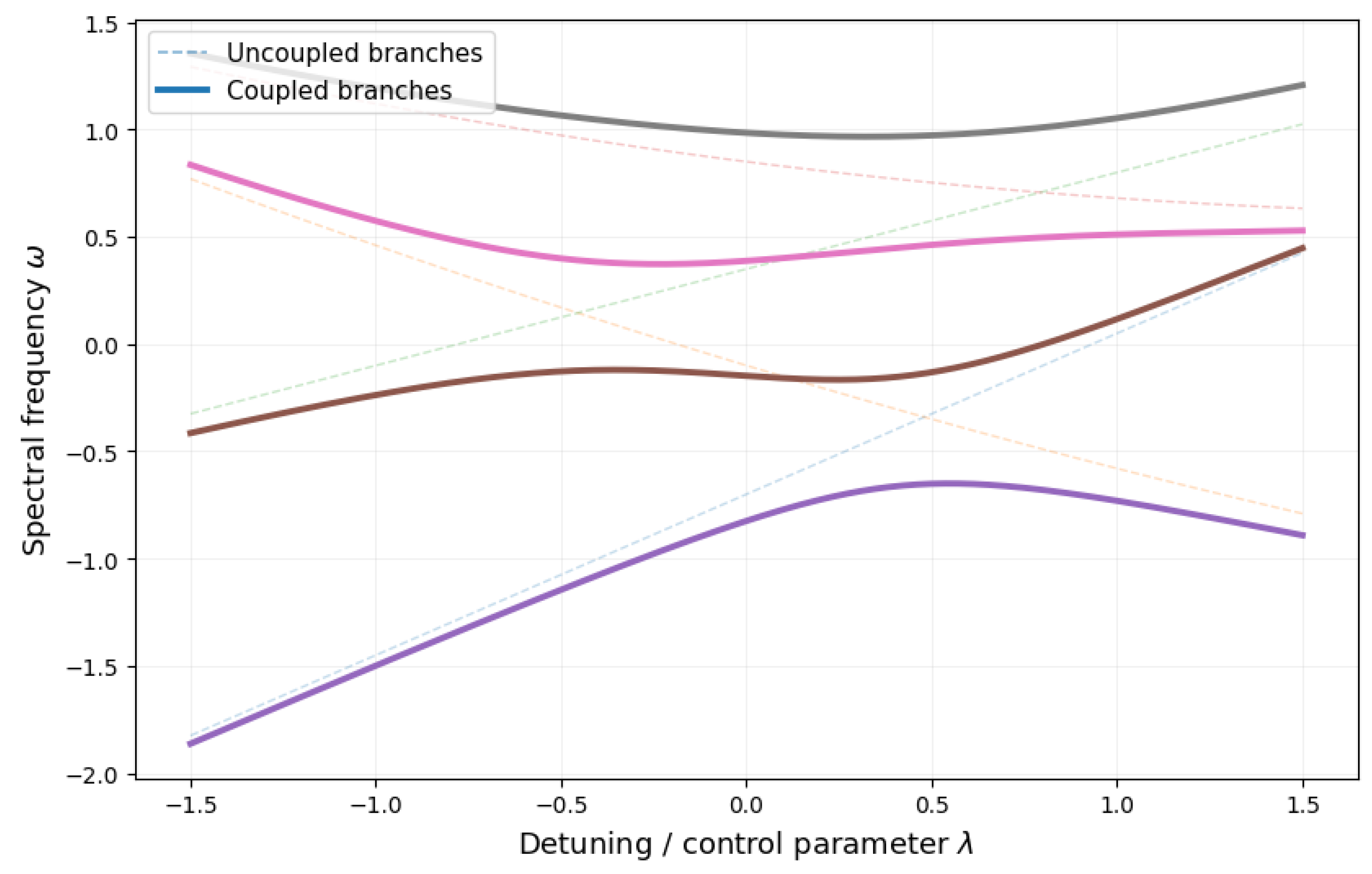
Although highly simplified, the two-channel and four-channel truncation captures the essential physics of the full matrix problem: the determinant condition encodes angular-channel mixing, and the resulting spectrum differs from that of any individual separated mode equations.
5.2. Boundary Response and Holographic Interpretation
The connection-coefficient formulation developed in the previous section makes explicit that the spectrum arises from global matching between regular throat solutions and asymptotic AdS behavior.
Near the AdS boundary, the scalar field decomposes into source and response components,
with the coefficients organized into vectors and matrices in angular-channel space. In the standard AdS/CFT interpretation, the slower falloff corresponds to non-normalizable source data, while the faster falloff corresponds to normalizable response data [39,41,50,51].
Because the rotating wormhole geometry mixes angular channels, source and response coefficients naturally organize into vectors in channel space. Bulk channel mixing therefore permits the response in one angular sector to depend on source data associated with other sectors. The boundary response function is therefore matrix-valued:
This is the coupled-channel analogue of the familiar ratio between normalizable and non-normalizable coefficients in a single-channel AdS spectral problem.
The pole structure of follows directly from the determinant condition. If , then becomes singular at . Equivalently, near an isolated simple pole, . Here is a coupled normal-mode frequency (pole location), and is the corresponding residue matrix.
In complex analysis, the residue measures the coefficient of the singular part of a function near a pole and therefore characterizes the local strength of the singular behavior. For example, if
then R is the residue associated with the pole at . Residues play a central role in contour integration, spectral theory, Green’s functions, and wave propagation because they determine how strongly a given pole contributes to the overall response. In physical systems, residues are often interpreted as measures of resonance strength or spectral weight. For instance, in a simple resonant oscillator or vibrating mechanical system, a larger residue corresponds to a stronger response near the natural frequency of the system. In this coupled-channel problem, the residue becomes matrix-valued because the collective normal modes can couple multiple angular harmonic sectors simultaneously.
The residue matrix encodes how strongly the pole couples different source and response channels. Its diagonal entries measure the response within a given angular sector, while its off-diagonal entries encode channel mixing in the boundary response.
For visualization, it is useful to evaluate the response slightly away from the real axis,
This does not mean that the physical normal-mode poles themselves have acquired imaginary parts or moved off the real frequency axis. Rather, the Green’s function is evaluated slightly above the real axis in the complex-frequency plane in order to regulate the pole singularities and render the spectral response finite and visually accessible.
In the self-adjoint wormhole problem, the poles remain on the real frequency axis. The small positive parameter instead acts as a regulator: it converts the singular pole
into the finite expression
Taking the imaginary part gives a Lorentzian peak,
centered at the real pole location .
Motivated by this standard pole expansion, we use the illustrative matrix-valued spectral model
The plotted quantity is
The trace is taken over the finite truncated channel basis introduced in Sec. 4, so that it sums the spectral response over the retained angular channels of the truncated coupled system, while the imaginary part displays the pole locations as finite Lorentzian peaks. The main conceptual advantage of this plot is that it provides a direct visual bridge between the abstract determinant condition and an observable spectral response function. As the angular-channel coupling increases, the collective normal-mode poles shift and separate through spectral repulsion, and this reorganization appears directly as a corresponding splitting and displacement of peaks in the matrix Green’s function. The figure therefore provides a spectral visualization of how the underlying coupled self-adjoint operator reorganizes the global normal-mode structure.
For the illustrative plot in Figure 4, the pole locations were chosen from the two-channel spectral mixing model of the previous subsection. The uncoupled poles were placed near two nearby normal-mode frequencies, and increasing the coupling parameter separates them according to the avoided-crossing structure discussed above. The residue matrices were chosen as simple positive channel-overlap matrices so that the trace response cleanly displays the coupled pole motion. The regulator was chosen small enough to keep the peaks narrow while still making them finite and visible.
It is important not to confuse the regulator with the channel-coupling parameter . The parameter controls physical angular-channel mixing in the spectral operator, whereas is a purely auxiliary quantity introduced to regulate the Green’s function near real-frequency poles. Thus, the figure is an illustrative spectral-response model, not a full numerical computation of the complete rotating AdS-Teo Green’s function.
This structure parallels the real-time holographic prescription of Son and Starinets [20] and its generalization to systems with operator mixing. The matrix structure reflects the fact that source and response data become coupled through the bulk angular-channel dynamics.
The determinant condition is therefore equivalent to the statement that the matrix Green’s function develops a pole. The bulk normal-mode spectrum is encoded in the analytic structure of the boundary response matrix.
To visualize the global evolution of the coupled spectral structure, we evaluate an illustrative determinant-response function for the same effective two-channel spectral model introduced in the previous subsection. The purpose of this model is not to compute the full rotating AdS-Teo wormhole spectrum numerically, but to display, in the simplest possible setting, how a matrix-valued quantization condition reorganizes spectral poles when angular channels are coupled.
For consistency, we use the same effective two-channel spectral model introduced previously, now interpreted from the perspective of the boundary response function. The poles of the matrix-valued response function therefore occur at the same frequencies determined by the two-channel spectral condition derived in Eq. (150). The corresponding pole branches are given by Eq. (164).
Specifically, we consider a frequency-dependent boundary coefficient matrix of the form
where and denote the uncoupled normal-mode frequencies associated with two independent angular channels. The parameter controls the strength of the channel mixing, while g sets the overall scale of the off-diagonal coupling.
The off-diagonal entries are chosen symmetrically as because the model is intended to represent a conservative self-adjoint coupled spectral problem. In such a system, the coupling from channel 1 to channel 2 equals the coupling from channel 2 to channel 1. This is the finite-dimensional analogue of a Hermitian matrix operator.
One could introduce more general off-diagonal entries, such as and . However, unless , the matrix would no longer be symmetric and would no longer represent the simplest conservative self-adjoint model. The choice is therefore the cleanest minimal choice for illustrating coupled spectral repulsion.
The word “motion” or “trajectory” refers here to the continuous change of the real-valued pole locations as the coupling strength is varied. In the self-adjoint wormhole problem, the poles remain on the real frequency axis; they do not acquire imaginary parts.
To display the same structure visually, we plot the diagnostic quantity
as a function of the real frequency and the coupling strength . Thus the horizontal axis of the plot is , the vertical axis is , and the color scale represents the value of Eq. (183).
The inverse determinant,
is large whenever the determinant is close to zero. Since the spectral poles occur at , this quantity acts as a convenient spectral-response diagnostic. The small positive regulator prevents the plotted quantity from diverging exactly at the poles, while the logarithm compresses the dynamic range so that the pole structure is visible in a color map.
As discussed earlier, the regulator should not be confused with the coupling parameter . The parameter controls physical angular-channel mixing, whereas merely regulates the response function near real-frequency poles.
The plotted quantity should therefore be understood as a visualization tool rather than a new fundamental observable. Purple regions correspond to weak response, whereas bright yellow ridges indicate frequencies at which approaches zero and the coupled spectral response is strongly enhanced.
The dashed white curves in the figure are the analytic pole trajectories obtained from the coupled spectral branches Eq. (164). Their agreement with the bright ridges shows that the color map is indeed visualizing the determinant zeros of the coupled response matrix.
A broader view of the coupled spectral structure is shown in Figure 5, where the determinant-response map traces the motion of the spectral poles as the channel-coupling strength varies.
The two-channel example illustrates this mechanism explicitly. The off-diagonal couplings shift the pole locations away from the frequencies associated with isolated channels, showing that the spectral poles are collective properties of the coupled system rather than attributes of individual angular modes.
Because the rotating AdS-Teo wormhole is smooth and horizonless, the resulting poles correspond to normal modes rather than dissipative quasinormal modes. The response structure therefore reflects a self-adjoint coupled spectral problem rather than the dissipative quasinormal-mode problem characteristic of black-hole scattering geometries.
This analysis assumes parameter regimes for which the rotating wormhole geometry remains free of ergoregion instabilities. In rotating horizonless spacetimes, sufficiently strong frame dragging together with reflective AdS boundary conditions can in principle lead to superradiant amplification and unstable modes. A detailed analysis of possible ergoregion instabilities lies beyond the scope of this work and would require a separate global study of the coupled rotating spectrum. Here we focus on the conservative coupled spectral structure associated with the self-adjoint regime of the problem.
To place the coupled-channel response of the rotating AdS-Teo wormhole in a broader context, it is useful to compare its spectral organization with the familiar quasinormal-mode structure of rotating black-holes.
In the wormhole case considered here, the boundary conditions consist of regularity at the throat together with AdS normalizability at the asymptotic boundaries. These conditions organize the scalar perturbation problem into an effectively self-adjoint coupled spectral system. Consequently, the normal-mode frequencies remain real in the stable regime, and angular-channel mixing manifests itself primarily through spectral repulsion and reorganization of the coupled eigenvectors.
By contrast, black-hole perturbations are governed by different boundary conditions. At the horizon, one imposes purely ingoing behavior, while at infinity one typically imposes outgoing or normalizable conditions, depending on the asymptotic structure of the spacetime. The resulting spectral problem is generally non-self-adjoint, and the associated frequencies become complex quasinormal modes,
whose imaginary parts describe the decay of perturbations through horizon absorption.
This distinction is illustrated schematically in Figure 6. The left panel represents the coupled normal-mode structure of the rotating AdS-Teo wormhole. The poles remain confined to the real frequency axis and undergo spectral repulsion as the angular-channel coupling increases. The right panel represents the qualitative behavior of black-hole quasinormal modes, whose frequencies occupy the lower half of the complex frequency plane due to dissipative horizon boundary conditions.
The purpose of this comparison is not to claim that the rotating wormhole spectrum is equivalent to a black-hole quasinormal spectrum. Rather, it emphasizes that the same mathematical language of poles, spectral flow, and response functions can arise in physically distinct settings. In this wormhole geometry, pole motion reflects the reorganization of a conservative coupled spectral system, whereas in black-hole spacetimes the corresponding pole structure is tied to dissipation and horizon absorption.
The comparison also clarifies the role of the determinant condition. In the wormhole problem, the determinant zeros identify normal-mode frequencies associated with a self-adjoint operator. The poles therefore remain on the real axis and correspond to collective oscillatory states of the coupled geometry. In black-hole problems, the analogous pole condition is typically imposed in a non-self-adjoint setting, leading instead to complex quasinormal frequencies.
Taken together, the Green’s-function response, determinant-response map, and spectral comparison provide three complementary perspectives on the same underlying physics. The matrix Green’s function emphasizes how collective poles appear in observable response functions. The determinant-response map visualizes the motion of those poles as angular-channel coupling is varied. The comparison with black-hole quasinormal modes highlights the role played by boundary conditions in determining whether the resulting spectral problem is conservative or dissipative.
From the holographic perspective, the matrix-valued response function suggests that non-separable bulk geometries naturally give rise to coupled boundary observables. The off-diagonal response channels provide a direct signature of angular-channel mixing in the bulk, while the determinant condition organizes the associated collective spectral structure. Although a complete holographic renormalization analysis lies beyond the scope of this work, the coupled response framework developed here provides a natural starting point for such investigations.
More broadly, this analysis demonstrates that the spectral consequences of non-separability can be studied through matrix-valued response functions in much the same way that ordinary normal modes and quasinormal modes are studied through scalar Green’s functions. The resulting picture is one in which interacting angular channels, rather than isolated harmonics, become the fundamental building blocks of the spectral response.
This viewpoint will play an important role in the discussion section, where we interpret the rotating AdS-Teo wormhole as a coupled spectral-operator system whose global normal modes, boundary response functions, and local quantum observables emerge collectively from the interaction of multiple angular sectors.
6. Boundary Observables
The previous sections established that the asymptotically AdS structure of the rotating AdS-Teo wormhole organizes the scalar field near the boundary into non-normalizable and normalizable branches. After projection onto angular harmonics, the corresponding asymptotic data are encoded in vectors
whose components label the coupled angular channels.
For a finite truncation to N angular channels, one constructs N linearly independent solutions regular at the throat and propagates them to the AdS boundary. Collecting the asymptotic coefficients column by column defines the matrices
The labels ± denote the even- and odd-parity sectors associated with reflection symmetry under .
In the standard AdS/CFT interpretation, the slower asymptotic falloff is identified with boundary source data, while the faster falloff is identified with the induced response [39,41,50,51]. In this work we use this source/response structure primarily as a diagnostic of the bulk wormhole geometry rather than assuming a fully specified microscopic dual theory.
A general throat-regular bulk solution is specified by a vector of coefficients
which determines the linear combination of regular basis solutions that is excited in the bulk. The corresponding boundary source and response vectors are therefore
Here represents the boundary source data and the induced boundary response.
Away from spectral zeros, the matrix is invertible, so
Substituting this relation into the expression for the response gives
The boundary Green’s function is therefore matrix-valued:
This is the natural coupled-channel generalization of the familiar single-channel relation
It is also the standard structure appearing in holographic systems with operator mixing, where coupled bulk fields lead to coupled boundary observables [20,21].
The pole structure of the boundary response follows directly from the global spectral problem. A source-free normal mode exists when there is a nontrivial vector such that
Equivalently,
At such frequencies, becomes singular, and the Green’s function develops a pole:
Thus the discrete bulk normal-mode spectrum is encoded in the analytic structure of the boundary response matrix.
Mathematically, the response matrix is a meromorphic function of the complex frequency . A meromorphic function is analytic everywhere except at isolated poles. Familiar examples include and , both of which are analytic except at discrete singular points. In this problem,
and since
the determinant appears in the denominator. Whenever , the inverse becomes singular and a pole develops. Thus the poles of the Green’s function coincide with the bulk normal-mode frequencies.
As discussed previously, the absence of an event horizon implies that the rotating AdS-Teo wormhole defines a conservative self-adjoint spectral problem whose poles correspond to normal modes rather than dissipative quasinormal modes.
The importance of self-adjointness may be seen directly from the eigenvalue equation
For a self-adjoint operator, , one finds
which implies
Hence the eigenvalues are real. In the current problem, this implies that the normal-mode frequencies remain confined to the real frequency axis.
By contrast, black-hole perturbations obey ingoing boundary conditions at the horizon. Energy can flow irreversibly into the horizon and is no longer returned to the exterior region. Mathematically, the resulting spectral problem is generally non-self-adjoint, so the spectral theorem no longer guarantees real eigenvalues. Complex frequencies become allowed,
leading to exponentially decaying quasinormal modes. Thus it is not “dissipation” itself that directly moves poles into the complex plane; rather, the dissipative boundary condition destroys self-adjointness, which in turn permits complex eigenvalues.
The response matrix is therefore meromorphic in the complex frequency plane, with isolated pole singularities associated with normal modes. More generally, spectral response functions may also exhibit branch cuts. Unlike a pole, which occurs at an isolated point, a branch cut arises when a function becomes multi-valued. Familiar examples include and . In spectral theory, branch cuts typically appear when a discrete set of modes is replaced by a continuum,
The resulting continuum integrals often generate logarithmic or square-root structures that are intrinsically multi-valued. To define these functions consistently as single-valued analytic objects, one introduces branch cuts in the complex plane. Such branch-cut behavior typically arises in continuum limits, noncompact scattering problems, or more generally whenever the spectrum contains a continuous set of states rather than a discrete set of isolated modes. This wormhole problem, however, is governed by a discrete AdS normal-mode spectrum, so the dominant analytic structure consists of isolated poles rather than branch cuts.
Angular-channel mixing nevertheless shifts the pole locations. In the two-channel truncation studied previously, the perturbative shift is controlled by Eq. (158). Thus the pole locations move along the real axis as the rotation-induced channel coupling is varied, rather than acquiring imaginary parts associated with damping.
For real background coefficients, the Green’s function satisfies the usual reality condition
so the spectrum exhibits the standard positive- and negative-frequency pairing.
Because the reflection-symmetric wormhole decomposes into even- and odd-parity sectors, the boundary response also decomposes:
The full response therefore takes the block-diagonal form
where ⊕ denotes a direct sum rather than an ordinary summation.
The symbol ⊕ denotes a direct sum rather than an ordinary summation. This distinction is important. An ordinary sum combines matrices element-by-element, whereas a direct sum places matrices into independent blocks. For example,
The resulting matrix is block diagonal: off-diagonal entries are allowed within each block, but there is no coupling between different blocks. In the current problem, the even- and odd-parity sectors form independent invariant subspaces, so the full Green’s function naturally decomposes into separate parity blocks. This block structure follows directly from the reflection symmetry . If reflection symmetry is broken, the parity sectors are no longer independent and the full response matrix ceases to be block diagonal.
The structure obtained here parallels the real-time holographic prescription of Son and Starinets, in which poles of boundary Green’s functions are associated with bulk normal or quasinormal frequencies [20]. The key distinction is that the AdS-Teo wormhole supports normal modes of a conservative two-boundary system, rather than dissipative horizon dynamics.
The matrix structure also parallels holographic operator-mixing calculations. In such systems, coupled bulk s imply that the boundary source and response data become vectors, and the Green’s function correspondingly becomes matrix-valued [21]. In this geometry, the axisymmetric wormhole background mixes angular harmonics, and the boundary response records both the spectrum and the angular-channel mixing.
The matrix structure of the response function therefore has a direct physical interpretation. In separable holographic systems, individual angular harmonics correspond to independent boundary operator sectors and the response matrix is diagonal. In this non-separable rotating wormhole geometry, however, rotation-induced channel mixing produces genuinely off-diagonal response components. The boundary observables therefore inherit the collective organization of the coupled bulk operator rather than decomposing into independent harmonic sectors.
In this sense, the holographic response is naturally matrix-valued and encodes the interacting structure of the coupled angular channels. Similar connections between bulk spectral structure, operator mixing, and matrix-valued response functions arise in holographic spectral analyses more broadly [20,52].
The boundary observables therefore provide a bridge between local throat dynamics and asymptotic response. The near-throat conformal organization discussed earlier constrains the local analytic structure of the coupled radial system, while global propagation to the AdS boundary determines the matrices and . The poles of encode the allowed normal-mode frequencies, while the matrix entries describe how angular channels mix as waves propagate from the throat to the asymptotic region.
In addition to these wave-based observables, the wormhole geometry admits a complementary semiclassical probe based on spacelike bulk geodesics connecting the two asymptotic boundaries. The relevant geodesics are spacelike because they approximate equal-time boundary two-point functions. Timelike geodesics describe massive particle motion in Lorentzian time, while null geodesics describe light propagation.
For boundary operators of large conformal dimension , the dominant contribution to the bulk path integral comes from the classical worldline saddle [53,54,55,56]. To understand this statement, consider the bulk propagator written schematically as a sum over all worldlines connecting two boundary points,
The path integral includes contributions from every possible path. However, when the bulk field is heavy,
the exponential strongly suppresses all trajectories except those near stationary points of the action. The dominant contribution therefore comes from the classical saddle satisfying
which is precisely the geodesic equation. In this limit, the path integral reduces to a geodesic approximation.
The corresponding two-boundary correlator takes the schematic form
where is the classical on-shell action evaluated on the spacelike geodesic. Here “on shell” means that the trajectory satisfies the classical geodesic equations.
For a point particle of mass m, the worldline action is
so evaluating the action on the geodesic gives
where is the proper geodesic length.
For a massive scalar in , the conformal dimension satisfies the indicial equation
This relation is obtained by inserting a power-law ansatz into the asymptotic radial wave equation and demanding consistency of the leading asymptotic behavior. For this geometry (), this reduces to the indicial equation derived earlier in Eq. (117).
In the heavy-field limit,
one obtains
Hence
and therefore
Because geodesic lengths diverge near the AdS boundary, one introduces a radial cutoff at and subtracts the universal AdS divergence [53,54,55,57]. The renormalized length is defined schematically by
The origin of the logarithm can be seen directly from the asymptotic AdS geometry. At large radius,
so the radial proper distance satisfies
Integrating gives
Using
one finds
For ,
which explains the subtraction term appearing in the renormalization procedure.
The semiclassical correlator therefore becomes
Eq. (222) is the standard geodesic approximation to the two-point function of heavy operators in AdS/CFT. Although derived from a bulk geodesic calculation, the result is expressed entirely in terms of boundary observables. This makes it a particularly useful probe of global geometric structure.
The key physical interpretation is that the correlator and the renormalized geodesic length contain equivalent information in the semiclassical limit. A shorter geodesic connecting the two boundaries produces a larger correlator, while a longer geodesic produces a more strongly suppressed correlator. Thus the boundary two-point function acts as a probe of the effective geometric separation between the two asymptotic regions.
In this wormhole geometry, the relevant geodesics traverse the interior region and connect the left and right AdS boundaries. The renormalized geodesic length therefore measures a genuinely global property of the spacetime rather than a local feature of the throat. Changes in the wormhole geometry are reflected directly in the corresponding boundary correlator.
To make this connection explicit, let
where is a reference geodesic length and represents a geometric perturbation induced by changes in the bulk spacetime. Expanding Eq. (222) gives
Even a modest change in the renormalized geodesic length can therefore produce a substantial change in the boundary correlator when the conformal dimension is large. Heavy operators are consequently particularly sensitive probes of global wormhole geometry.
The geodesic approximation should be viewed as complementary to the matrix-valued Green’s function analysis discussed earlier. The Green’s function probes the spectral organization of coupled scalar modes, whereas the geodesic correlator probes the global geometric connectivity of the spacetime. Together they provide two distinct windows into the same underlying wormhole structure.
From the holographic perspective, Eq. (222) provides an explicit example of a bulk-boundary correspondence. The quantity is a bulk geometric observable: it is computed entirely from the geometry of spacelike geodesics propagating through the wormhole interior. By contrast, is a boundary observable defined solely in terms of operators living on the asymptotic conformal boundaries.
Eq. (222) therefore demonstrates how information about the bulk geometry can be encoded in a boundary correlation function. Although considerably simpler than a complete bulk reconstruction program, it captures the central holographic idea that geometric properties of the interior spacetime may be inferred from observables defined entirely on the boundary.
This observation is particularly natural in a two-boundary wormhole geometry. The correlator directly probes the existence of spacelike paths connecting the two asymptotic regions. The corresponding renormalized geodesic length measures the effective geometric distance through the bulk, while the boundary correlator measures the strength of the associated cross-boundary correlation.
The result should therefore be interpreted not merely as a convenient computational approximation, but as a concrete illustration of how bulk and boundary descriptions become related in asymptotically AdS spacetimes. The wormhole geometry determines the geodesic structure; the geodesic structure determines ; and in turn controls the asymptotic boundary correlator.
Taken together, the matrix-valued response functions and geodesic correlators provide complementary probes of the rotating AdS-Teo wormhole. The response matrices encode the coupled spectral structure of scalar perturbations and reveal how angular-channel mixing reorganizes the normal-mode spectrum. The geodesic correlators probe global connectivity and encode geometric information about the wormhole interior through boundary observables. Both perspectives illustrate how non-separability, global geometry, and asymptotic AdS structure combine to produce a rich set of boundary signatures of the rotating wormhole spacetime.
These results suggest that the rotating AdS-Teo wormhole may serve as a useful laboratory for studying how coupled spectral systems, matrix-valued response functions, and geometric probes are organized in non-separable horizonless spacetimes. A more complete holographic analysis, including holographic renormalization and a detailed study of the associated boundary operator structure, would be an interesting direction for future work.
7. Local Vacuum Polarization Near the Throat
As an additional local probe of the rotating AdS–Teo wormhole, we consider the renormalized vacuum polarization, . Unlike the boundary response functions discussed in Sec. VI, this local observable probes how the coupled bulk geometry modifies vacuum fluctuations at a spacetime point. Unlike the boundary response functions discussed in Sec. VI, this quantity measures quantum fluctuations at a spacetime point and therefore probes how the coupled bulk geometry modifies the local vacuum structure. Because the throat is the region where the two asymptotic AdS regions are joined and where the effects of curvature, rotation, and angular-channel mixing are most pronounced, it provides a natural location in which to study this observable.
Throughout this section we assume that the quantum state is of Hadamard form, so that the short-distance singularity of the two-point function has the universal local structure required in curved-spacetime quantum field theory [5,6]. The renormalized quantity is obtained by the standard point-splitting and Hadamard subtraction procedure. Although a complete semiclassical analysis would ultimately require the renormalized stress tensor , the vacuum polarization already captures the renormalized two-point structure from which the stress tensor may be constructed by further differentiation [5,6,58].
7.1. Coupled Mode Expansion and Wightman Function
The scalar-field modes were constructed in the previous sections by solving the coupled-channel spectral problem. A physical normal mode is therefore not generally a single separated product , but rather a linear combination of angular channels.
For a normal mode labeled by
where n labels the discrete normal-mode frequency, m is the azimuthal number, and p denotes the even- or odd-parity sector, we write the spatial mode profile as
The functions are the radial components in each angular channel, are the polar harmonics, and the coefficients determine how strongly each angular channel contributes to the coupled physical mode. These are therefore not weights of independent uncoupled eigenmodes. Rather, they are the components of the coupled normal-mode eigenvector when expressed in the angular-channel basis.
These coefficients are determined by the global spectral problem. For a fixed parity sector, the allowed frequencies satisfy
At such a frequency there exists a nontrivial vector such that
The channel weights are precisely the components of this null vector:
The positive-frequency mode function is therefore
with normalization constant . Substituting Eq. (226) into Eq. (230) gives
The scalar field operator is expanded as
The vacuum is defined by
The Wightman function is
Substituting for and from Eq. (232), one obtains
Expanding the product,
Since , all terms vanish except
Therefore
Substituting the coupled-channel expansion,
and similarly for the complex conjugate profile, gives
The Wightman function therefore becomes
The double sum over is the local imprint of angular-channel mixing. In a fully separable geometry, a physical mode occupies only one angular channel and the off-diagonal contributions with are absent. In the rotating AdS-Teo wormhole, by contrast, each normal mode is generally a coherent superposition of several angular channels. The two-point function therefore contains both diagonal channel contributions and interference terms between distinct angular sectors.
Physically, measures the vacuum correlation between scalar-field fluctuations at the two spacetime points x and . The result above shows that these correlations are not merely sums over independent separated harmonics. Instead, they retain information about the coupled spectral structure of the rotating wormhole geometry. The off-diagonal terms in the sum provide a local quantum signature of non-separability: they show that vacuum fluctuations in one angular sector are correlated with fluctuations in other sectors through the geometry-induced channel mixing.
7.2. Coincident Limit and Hadamard Subtraction
The coincident limit means bringing the second spacetime point to the first:
The formal limit of is ultraviolet divergent because the quantum field fluctuates at arbitrarily short distances.
The renormalized vacuum polarization is defined by point splitting:
where is the universal Hadamard singular term.
Here point splitting and Hadamard subtraction refer to two closely related parts of the same renormalization procedure. Point splitting means that one first keeps the two spacetime points x and distinct, so that the two-point function is well-defined away from coincidence. Hadamard subtraction then removes the universal short-distance singular part of the two-point function before the limit is taken. Thus point splitting is the regulator, while Hadamard subtraction is the covariant subtraction prescription.
For a Hadamard state in four spacetime dimensions, the singular part of the two-point function has the universal local form [5,31,58]
This expression is not derived from the global normal-mode spectrum. Rather, it is the standard local Hadamard parametrix: it is obtained by solving the wave equation locally near coincidence and expanding the two-point function in powers of the geodesic separation. Here is Synge’s world function, equal to one half of the squared geodesic distance between the two points, while and are smooth biscalars determined recursively by the local geometry, curvature, mass, and curvature coupling [59,60,61].
The subtraction term is universal: it depends only on the local short-distance geometry and not on whether the global modes are separable or coupled. Consequently, the coupled-channel physics enters only through the finite, state-dependent remainder of the mode sum, whereas the Hadamard singular term is determined entirely by the local geometry. For this reason we do not require the full closed form of and for the rotating AdS-Teo geometry in this illustrative calculation. A full numerical computation of would require evaluating the appropriate DeWitt-Schwinger or Hadamard subtraction terms for the specific metric, as is done in explicit curved-spacetime calculations of vacuum polarization and stress tensors [58,62].
Using Eq. (240) in Eq. (245), and keeping the points separated until after the Hadamard subtraction is performed, we may choose equal time and equal azimuthal angle for notational simplicity while retaining the remaining point-splitting regulator. This gives
Substituting the coupled-channel expansion,
The subtraction must be performed before the coincidence limit is taken. If one first sets , the mode sum and the singular term are separately divergent. Keeping x and distinct allows the universal divergent part of the two-point function to be identified and removed covariantly. Only after this cancellation is the limit finite and physically meaningful.
7.3. Explicit Regularization and Physical Interpretation
To evaluate the renormalized quantity more explicitly, it is convenient to introduce a small Euclidean time separation,
while keeping the spatial coordinates fixed. This regulates the mode sum by exponentially suppressing large frequencies:
Using Eq. (240), the regulated Wightman function becomes
Substituting the coupled-channel expansion,
gives
For a small Euclidean time separation at fixed spatial position, the geodesic interval is locally
up to curvature corrections. Since Synge’s world function is one half of the squared geodesic distance, we have Also,
Therefore, the leading Hadamard singularity becomes
Thus,
The logarithmic terms contain curvature- and mass-dependent local contributions. They are included in the full Hadamard subtraction, but the leading term is sufficient to display the origin of the ultraviolet divergence. The renormalized vacuum polarization is therefore
Substituting Eq. (253),
At this stage the Hadamard term has already been isolated as the subtraction term in Eq. (257). The remaining channel decomposition refers to the regulated mode sum inside the square brackets. The mode sum naturally separates into diagonal and off-diagonal channel contributions:
The diagonal part of the regulated mode sum is
while the off-diagonal part is
Thus, the renormalized quantity is schematically
The singular Hadamard subtraction is local and universal; the diagonal and off-diagonal decomposition describes the finite coupled-channel structure of the regulated mode sum.
These interference terms are the direct local signature of non-separability. In a separable geometry, a physical mode occupies a single angular channel and all off-diagonal contributions vanish.
To illustrate the structure concretely, consider again the two-channel truncation involving channels L and . The mode profile becomes
Squaring the profile,
The final two terms are interference contributions between the angular channels. Writing them explicitly as a real part,
Substituting Eq. (264) into the regulated mode sum gives
Equivalently, the regulated two-channel contribution may be written as
where the interference term is
The corresponding renormalized vacuum polarization is therefore
This form makes clear that the Hadamard term has not disappeared: it subtracts the universal coincident-point divergence from the total regulated two-channel mode sum. The interference term is a finite state-dependent contribution produced by channel mixing.
Near the throat, parity further constrains the local structure. For an even mode,
while for an odd mode,
At the throat, , the interference structure depends strongly on the parity sector. In particular, odd modes vanish directly at the throat, while even modes remain finite there.
To illustrate how angular-channel mixing can modify local quantum observables, we plot a schematic finite-mode model inspired by Eq. (268). The plotted profile is not a full numerical evaluation of the renormalized stress tensor or of the complete Hadamard-subtracted mode sum in the rotating AdS-Teo geometry. Instead, it isolates the finite coupled-channel part of the vacuum-polarization profile after the universal short-distance divergence has been subtracted.
An illustrative realization of this finite coupled-channel vacuum-polarization profile is shown schematically in Figure 7, where the off-diagonal interference term produces the localized oscillatory structure near the wormhole throat.
For the illustrative plot, we use model throat-centered radial profiles and , together with simple channel weights and , and form a finite expression of the schematic form
where and represent diagonal channel contributions and represents the off-diagonal interference profile. The parameter controls the strength of the channel-mixing contribution. Increasing therefore enhances the interference term and produces the localized oscillatory structure visible near the throat.
The renormalized vacuum polarization thus provides a local probe of the global coupled-channel structure developed throughout the paper. Although the Hadamard subtraction removes the universal ultraviolet divergence, the finite renormalized remainder retains detailed information about angular mixing, parity structure, and global spectral matching.
A complete semiclassical analysis would require the renormalized stress tensor , which is obtained from derivatives of the point-split Green function. The interference terms identified above suggest that the renormalized stress tensor may inherit nontrivial anisotropic structure near the throat, reflecting the coupled angular dynamics of the rotating wormhole geometry.
In summary, the rotating AdS-Teo wormhole differs qualitatively from both static, spherically symmetric wormholes and separable rotating black-holes. The physical scalar field modes are collective coupled-channel excitations rather than independent angular harmonics, and this non-separable structure leaves a direct imprint not only on the global normal-mode spectrum but also on local quantum observables through the interference terms appearing in .
8. Discussion and Outlook
In this work, we have formulated a coupled spectral framework for scalar perturbations in the rotating AdS-Teo wormhole. The analysis combines global spectral theory, near-throat operator structure, holographic response, and local quantum observables in a generically non-separable, axisymmetric geometry.
The principal conceptual result of this work is that, in the absence of complete separability, the natural organizing framework for wave dynamics is not a collection of independent mode equations but a coupled-channel spectral theory. Rather than treating angular harmonics as isolated sectors, the rotating AdS-Teo wormhole organizes them into interacting spectral channels whose collective behavior determines the normal-mode spectrum, boundary response functions, and local quantum observables. In this sense, coupled-channel spectral theory replaces separability as the fundamental organizing principle for this class of rotating horizonless geometries.
A central result is that the scalar-field equation does not generally separate in the rotating wormhole background. Expanding the field in angular harmonics therefore leads not to independent radial equations, but to a matrix-valued coupled system in which different angular sectors interact through the geometry. The resulting spectral problem is intrinsically multi-channel and is naturally formulated as a matrix-valued Sturm-Liouville problem.
The physical spectrum is determined globally by matching regular throat solutions to asymptotically AdS boundary conditions. A nontrivial linear combination of throat-regular solutions must become purely normalizable at the AdS boundary, leading to the determinant quantization condition
This generalizes the familiar single-channel condition encountered in fully separable systems.
The physical consequences of angular-channel mixing were illustrated explicitly through a two-channel truncation, where the coupled structure induces shifts in the normal-mode frequencies, produces spectral repulsion, and reorganizes the corresponding eigenvectors into collective modes. The spectrum is therefore a collective property of the coupled system rather than a feature of isolated angular sectors.
A noteworthy conceptual outcome of this analysis is that the coupled-channel formulation is not merely a technical reorganization of the scalar-field , but a qualitatively different framework for describing wave dynamics in non-separable geometries. Rather than treating angular harmonics as independent sectors, the physically relevant degrees of freedom are collective excitations built from interacting channels. The determinant condition therefore becomes the fundamental spectral object, encoding the global quantization of the coupled system through a matrix-valued operator. From this perspective, non-separable rotating wormhole geometries are most naturally understood through the spectral theory of coupled operators, in which the spectrum emerges collectively from matrix-valued quantization conditions and both bulk and boundary observables inherit an intrinsically coupled analytic structure.
The coupled spectral framework developed in this work differs qualitatively from dissipative black-hole quasinormal-mode problems: the horizonless wormhole geometry remains self-adjoint under AdS boundary conditions, leading to real normal-mode frequencies rather than damped complex resonances.
At the level of boundary observables, the asymptotic data organize into a matrix-valued response function,
whose poles coincide with the bulk normal-mode frequencies. The off-diagonal components encode angular-channel mixing and therefore provide a direct boundary signature of the non-separable rotating geometry.
From this perspective, the boundary response matrix contains information beyond the locations of spectral poles. The residue structure and off-diagonal response components encode how individual angular channels participate in a collective mode. Consequently, the boundary observables inherit the same coupled spectral organization that characterizes the bulk dynamics.
An important feature of this framework is that the same channel-mixing structure appears in several apparently different observables. At the spectral level, it enters through the determinant quantization condition . At the boundary, it appears through the matrix-valued response function . Locally, it manifests itself through interference terms in the renormalized vacuum polarization. These descriptions are not independent; rather, they represent complementary manifestations of the same underlying coupled-channel dynamics.
Because the spacetime is smooth and horizonless, the spectral problem remains conservative and self-adjoint under the throat and AdS boundary conditions. Consequently, the poles correspond to normal modes rather than dissipative quasinormal modes. This sharply distinguishes this system from rotating black-hole geometries, where horizon absorption leads to complex quasinormal frequencies.
More generally, this analysis highlights the close relationship between spectral structure, boundary conditions, and the mathematical properties of the underlying differential operator. In the asymptotically AdS wormhole geometry, the reflective boundary conditions together with throat regularity organize the coupled radial system into an effectively self-adjoint matrix Sturm-Liouville problem with a discrete real spectrum. From this perspective, the resulting normal modes are naturally interpreted as collective bound-state oscillations of a confined coupled system. By contrast, in open geometries with radiative or horizon-absorbing boundary conditions, the corresponding spectral problem becomes non-self-adjoint and the poles move into the complex frequency plane, producing dissipative resonances and quasinormal-mode behavior. The distinction between normal modes and quasinormal modes therefore reflects not only differences in geometry, but also deeper differences in how boundary conditions organize the spectral theory of wave operators in curved spacetime.
The framework developed here is not tied specifically to the rotating AdS-Teo wormhole. More generally, it suggests that coupled-channel spectral theory may provide a useful organizing principle for a broader class of rotating or non-separable geometries in which conventional mode separability fails. From this perspective, the rotating AdS-Teo wormhole serves as a concrete example of a wider operator-theoretic structure whose manifestations include collective normal modes, matrix-valued response functions, and coupled quantum observables.
Near the throat, we identified a local conformal-type organization of the radial operator. Unlike hidden conformal structures associated with black-hole horizons, this structure arises at a regular interior point and acts on a vector of coupled channels. It therefore organizes the local solution space without determining the global spectrum. The near-throat analysis thus provides a local organizing principle for the coupled-channel dynamics, while the full spectrum remains determined by the global matching problem connecting the throat region to the asymptotic AdS boundaries.
We also constructed the coupled-channel Wightman function and analyzed the renormalized vacuum polarization . The resulting expressions contain interference terms between angular channels, providing a local quantum signature of non-separability. Such interference terms are absent in fully separable geometries and therefore distinguish the rotating wormhole from both spherically symmetric wormholes and Kerr-type separable backgrounds.
The appearance of interference terms in is particularly significant because it demonstrates that the effects of angular-channel coupling are not confined to the global spectrum. Rather, channel mixing leaves a local imprint on quantum observables after the universal Hadamard short-distance singularity has been removed. In this sense, the renormalized vacuum polarization provides an independent diagnostic of non-separability that complements both the spectral analysis and the boundary response function.
In addition to the wave-based observables, we studied a complementary semiclassical probe based on spacelike geodesics connecting the two asymptotic AdS boundaries. In the large- limit, the cross-boundary correlator is controlled by the renormalized geodesic length,
providing a geometric diagnostic of two-boundary connectivity that is complementary to the coupled spectral analysis. Unlike the matrix-valued response function, which probes the spectral organization of bulk wave excitations, the geodesic observable provides a direct measure of the underlying geometric connectivity between the two asymptotic regions. Together, these observables illustrate how both wave dynamics and semiclassical probes encode information about the global wormhole structure.
The framework developed here opens several directions for future investigation. A numerical analysis of the full coupled spectral problem would permit explicit computation of the normal-mode spectrum and quantitative study of angular-channel mixing beyond the illustrative two-channel truncation shown here. More generally, extending the determinant formulation to larger channel spaces may reveal richer patterns of spectral reorganization, including multi-channel avoided crossings, collective mode formation, residue-matrix evolution, and more intricate matrix-valued response structures. Such investigations may help clarify how spectral information is distributed among interacting angular sectors in strongly coupled non-separable geometries.
The coupled-channel construction of the Wightman function further provides the starting point for computation of the renormalized stress-energy tensor . Such an analysis would permit a fully semiclassical study of backreaction and may reveal anisotropic quantum effects near the throat arising from channel interference. The vacuum polarization results shown here therefore represent a first step toward a broader semiclassical treatment of quantum fields in rotating non-separable wormhole backgrounds.
The matrix-valued response structure further suggests possible connections with holographic systems exhibiting operator mixing. A more complete holographic treatment, including boundary counterterms, holographic renormalization, and a detailed analysis of the matrix-valued correlator structure, may help clarify whether the rotating AdS-Teo geometry admits a useful dual field-theoretic interpretation. Although this work does not establish a complete holographic duality, the response framework developed here provides a natural language for exploring such questions.
It would also be interesting to investigate whether analogous coupled spectral structures arise in other non-separable geometries, including rotating wormholes with different asymptotics, higher-spin fields, Dirac perturbations, vector and tensor modes, or geometries supported by more general matter sources. From this perspective, the coupled-channel formulation developed here may prove useful beyond the specific rotating AdS-Teo background considered in this work.
More broadly, this work suggests that rotating horizonless spacetimes lacking sufficient symmetry for complete separation of variables must be formulated as coupled-channel systems rather than as collections of independent mode equations. In such geometries, the wave equation is intrinsically matrix-valued, and any reduction to a single-channel description necessarily represents a controlled approximation obtained through truncation or projection. The rotating AdS-Teo wormhole therefore provides a useful theoretical laboratory for investigating how geometry, boundary conditions, and operator structure combine to produce collective spectral behavior. Although the analysis done here is restricted to scalar fields in the rotating AdS-Teo geometry, the underlying mathematical framework is expected to apply much more broadly to non-separable wave equations in curved spacetime.
From this perspective, the principal result of this work is not merely the identification of a particular spectrum, but the development of a unified coupled-channel spectral framework that connects global quantization conditions, matrix-valued boundary response functions, and local quantum observables within a single non-separable gravitational system. The rotating AdS-Teo wormhole provides an explicit example in which collective normal modes, coupled boundary responses, and local quantum interference effects all emerge from the same underlying channel-mixing structure. More generally, our results suggest that coupled-channel spectral theory constitutes the natural mathematical framework for non-separable gravitational systems, where the fundamental dynamical objects are collective excitations of the full coupled operator rather than isolated mode sectors.
References
- Parker, L. Quantized Fields and Particle Creation in Expanding Universes. I. Phys. Rev. 1969, 183, 1057–1068. [Google Scholar] [CrossRef]
- Fulling, S.A. Nonuniqueness of Canonical Field Quantization in Riemannian Space-Time. Phys. Rev. D. 1973, 7, 2850–2862. [Google Scholar] [CrossRef]
- Unruh, W.G. Notes on Black-Hole Evaporation. Phys. Rev. D. 1976, 14, 870–892. [Google Scholar] [CrossRef]
- Hawking, S.W. Particle Creation by Black Holes. Commun. Math. Phys. 1975, 43, 199–220. [Google Scholar] [CrossRef]
- Birrell, N.D.; Davies, P.C.W. Quantum Fields in Curved Space; Cambridge University Press, 1982. [Google Scholar]
- Wald, R.M. Quantum Field Theory in Curved Spacetime and Black Hole Thermodynamics; University of Chicago Press, 1994. [Google Scholar]
- Berti, E.; Cardoso, V.; Starinets, A.O. Quasinormal modes of black holes and black branes. Living Rev. Relativ. 2009, 12, 6. [Google Scholar]
- Teukolsky, S.A. Perturbations of a rotating black hole. I. Fundamental equations for gravitational, electromagnetic, and neutrino-field perturbations. Astrophys. J. 1973, 185, 635–647. [Google Scholar] [CrossRef]
- Carter, B. Global Structure of the Kerr Family of Gravitational Fields. Phys. Rev. 1968, 174, 1559–1571. [Google Scholar] [CrossRef]
- Chandrasekhar, S. The Mathematical Theory of Black Holes; Oxford University Press, 1983. [Google Scholar]
- Guica, M.; Hartman, T.; Song, W.; Strominger, A. The Kerr/CFT Correspondence. Phys. Rev. D. 2009, 80, 124008, [0809.4266. [Google Scholar] [CrossRef]
- Castro, A.; Maloney, A.; Strominger, A. Hidden Conformal Symmetry of the Kerr Black Hole. Phys. Rev. D. 2010, 82, 024008, [1004.0996. [Google Scholar] [CrossRef]
- Morris, M.S.; Thorne, K.S. Wormholes in Spacetime and Their Use for Interstellar Travel: A Tool for Teaching General Relativity. Am. J. Phys. 1988, 56, 395–412. [Google Scholar] [CrossRef]
- Visser, M. Lorentzian Wormholes: From Einstein to Hawking; Springer, 1995. [Google Scholar]
- Teo, E. Rotating Traversable Wormholes. Phys. Rev. D. 1998, 58, 024014, [gr–qc/9803098. [Google Scholar] [CrossRef]
- Newton, R.G. Scattering Theory of Waves and Particles, 2 ed.; Springer: New York, 1982. [Google Scholar]
- Taylor, J.R. Scattering Theory: The Quantum Theory of Nonrelativistic Collisions; Dover Publications: Mineola, New York, 2006. [Google Scholar]
- Zettl, A. Sturm–Liouville Theory. In Mathematical Surveys and Monographs; American Mathematical Society, 2005; Vol. 121. [Google Scholar]
- Teschl, G. Mathematical Methods in Quantum Mechanics, 2 ed.; American Mathematical Society, 2014. [Google Scholar]
- Son, D.T.; Starinets, A.O. Minkowski-space correlators in AdS/CFT. JHEP 2002, 09, 042. [Google Scholar] [CrossRef]
- Kaminski, M.; Landsteiner, K.; Mas, J.; Shock, J.P.; Tarrio, J. Holographic Operator Mixing and Quasinormal Modes on the Brane. JHEP 2010, 02, 021. [Google Scholar] [CrossRef]
- Amado, I.; Kaminski, M.; Landsteiner, K. Hydrodynamics of Holographic Superconductors. JHEP 2010, arXiv:hep05, 021. [Google Scholar]
- Futterman, J.A.H.; Handler, F.A.; Matzner, R.A. Scattering from Black Holes; Cambridge University Press, 1988. [Google Scholar]
- Avis, S.J.; Isham, C.J.; Storey, D. Quantum field theory in anti-de Sitter space-time. Phys. Rev. D. 1978, 18, 3565–3576. [Google Scholar] [CrossRef]
- Ishibashi, A.; Wald, R.M. Dynamics in non-globally-hyperbolic spacetimes. Class. Quant. Grav. 2004, 21, 2981–3014. [Google Scholar] [CrossRef]
- Holzegel, G.; Warnick, C. The Einstein-Klein-Gordon-AdS system. [CrossRef] [PubMed]
- Wald, R.M. General Relativity; University of Chicago Press, 1984. [Google Scholar]
- Carroll, S.M. Spacetime and Geometry: An Introduction to General Relativity; Addison-Wesley, 2004. [Google Scholar]
- Hawking, S.W.; Ellis, G.F.R. The Large Scale Structure of Space-Time; Cambridge Monographs on Mathematical Physics: Cambridge; Cambridge University Press, 1973. [Google Scholar] [CrossRef]
- Penrose, R.; Rindler, W. Spinors and Space-Time. In Cambridge Monographs on Mathematical Physics; Cambridge University Press: Cambridge, 1984; Volume 1. [Google Scholar]
- Wald, R.M. Quantum Field Theory in Curved Spacetime and Black Hole Thermodynamics; University of Chicago Press, 1994. [Google Scholar]
- Krishnan, C.; Pathak, P.S. Normal modes of the stretched horizon: a bulk mechanism for black hole microstate level spacing. J. High Energy Phys. 2024, arXiv:hep, 2024, 162. [Google Scholar] [CrossRef]
- Naimark, M.A. Linear Differential Operators; Ungar, 1967. [Google Scholar]
- Weidmann, J. Spectral Theory of Ordinary Differential Operators; Springer, 1987. [Google Scholar]
- Weigel, H.; Quandt, M.; Graham, N. Spectral methods for coupled channels with a mass gap. Phys. Rev. D. 2018, 97. [Google Scholar] [CrossRef]
- Brown, J.D.; Henneaux, M. Central Charges in the Canonical Realization of Asymptotic Symmetries: An Example from Three-Dimensional Gravity. Commun. Math. Phys. 1986, 104, 207–226. [Google Scholar] [CrossRef]
- Courant, R.; Hilbert, D. Methods of Mathematical Physics; Wiley, 1953. [Google Scholar]
- Gubser, S.S.; Klebanov, I.R.; Polyakov, A.M. Gauge Theory Correlators from Non-Critical String Theory. Phys. Lett. B 1998, 428, 105–114, [hep-th/9802109. [Google Scholar] [CrossRef]
- Witten, E. Anti-de Sitter space and holography. Adv. Theor. Math. Phys. 1998, 2, 253–291. [Google Scholar] [CrossRef]
- Klebanov, I.R.; Witten, E. AdS/CFT Correspondence and Symmetry Breaking. Nucl. Phys. B 1999, 556, 89–114. [Google Scholar] [CrossRef]
- Skenderis, K. Lecture notes on holographic renormalization. Class. Quant. Grav. 2002, 19, 5849–5876. [Google Scholar] [CrossRef]
- Boyd, J.P. Chebyshev and Fourier Spectral Methods, 2 ed.; Dover Publications, 2001. [Google Scholar]
- Canuto, C.; Hussaini, M.Y.; Quarteroni, A.; Zang, T.A. Spectral Methods: Fundamentals in Single Domains; Springer, 2006. [Google Scholar]
- Arnold, V.I. Mathematical Methods of Classical Mechanics. In Graduate Texts in Mathematics, 2 ed.; Springer-Verlag: New York, 1989; Vol. 60. [Google Scholar]
- Wald, R.M. General Relativity; University of Chicago Press: Chicago, IL, 1984. [Google Scholar]
- Kokkotas, K.D.; Schmidt, B.G. Quasinormal modes of stars and black holes. Living Rev. Relativ. 1999, 2, 2. [Google Scholar] [CrossRef] [PubMed]
- Messiah, A. Quantum Mechanics; North-Holland, 1961. [Google Scholar]
- Hatsuda, Y.; Kimura, M. Spectral Problems for Quasinormal Modes of Black Holes. Universe 2021, arXiv:gr7, 476. [Google Scholar] [CrossRef]
- Sakurai, J.J.; Napolitano, J. Modern Quantum Mechanics, 2 ed.; Cambridge University Press, 2017. [Google Scholar]
- Maldacena, J. The Large N limit of superconformal field theories and supergravity. Adv. Theor. Math. Phys. 1998, 2, 231–252. [Google Scholar] [CrossRef]
- Aharony, O.e.a. Large N field theories, string theory and gravity. Phys. Rept. 2000, 323, 183–386. [Google Scholar] [CrossRef]
- Hartnoll, S.A. Lectures on holographic methods for condensed matter physics. Class. Quantum Gravity 2009, 26, 224002. [Google Scholar] [CrossRef]
- Balasubramanian, V.; Ross, S.F. Holographic particle detection. Phys. Rev. D. 2000, 61, 044007. [Google Scholar] [CrossRef]
- Louko, J.; Marolf, D.; Ross, S.F. On Geodesic Propagators and Black Hole Holography. Phys. Rev. D. 2000, 62, 044041. [Google Scholar] [CrossRef]
- Aparicio, L.; Lopez, E. Evolution of Two-Point Functions from Holography. JHEP 2011, arXiv:hep12, 082. [Google Scholar] [CrossRef]
- Hartman, T.; Maldacena, J. Time Evolution of Entanglement Entropy from Black Hole Interiors. JHEP 2013, arXiv:hep05, 014. [Google Scholar] [CrossRef]
- Festuccia, G.; Liu, H. Excursions beyond the horizon: Black hole singularities in Yang-Mills theories. JHEP 2006, 04, 044. [Google Scholar] [CrossRef]
- Décanini, Y.; Folacci, A. Hadamard renormalization of the stress-energy tensor for a quantized scalar field in a general spacetime of arbitrary dimension. Phys. Rev. D. 2008, 78, 044025. [Google Scholar] [CrossRef]
- DeWitt, B.S. Quantum Theory of Gravity. III. Applications of the Covariant Theory. Phys. Rev. 1967, 162, 1239–1256. [Google Scholar] [CrossRef]
- Christensen, S.M. Vacuum Expectation Value of the Stress Tensor in an Arbitrary Curved Background: The Covariant Point-Separation Method. Phys. Rev. D. 1976, 14, 2490–2501. [Google Scholar] [CrossRef]
- Poisson, E.; Pound, A.; Vega, I. The Motion of Point Particles in Curved Spacetime. Living Rev. Relativ. 2011, 14, 7. [Google Scholar] [CrossRef] [PubMed]
- Taylor, B.E.; Hiscock, W.A.; Anderson, P.R. gr-qc/9608036; Stress-energy of a quantized scalar field in static wormhole spacetimes. 1996.
Figure 1.
Illustrative eigenvalues of a two-channel effective potential matrix near the wormhole throat. Dashed curves denote the uncoupled channel potentials, while solid curves show the eigenvalues of the coupled matrix-valued operator. Angular-channel mixing reorganizes the local propagation problem into coupled effective channels and produces level repulsion near the throat region. The vertical dotted line indicates the location of the wormhole throat at .
Figure 1.
Illustrative eigenvalues of a two-channel effective potential matrix near the wormhole throat. Dashed curves denote the uncoupled channel potentials, while solid curves show the eigenvalues of the coupled matrix-valued operator. Angular-channel mixing reorganizes the local propagation problem into coupled effective channels and produces level repulsion near the throat region. The vertical dotted line indicates the location of the wormhole throat at .
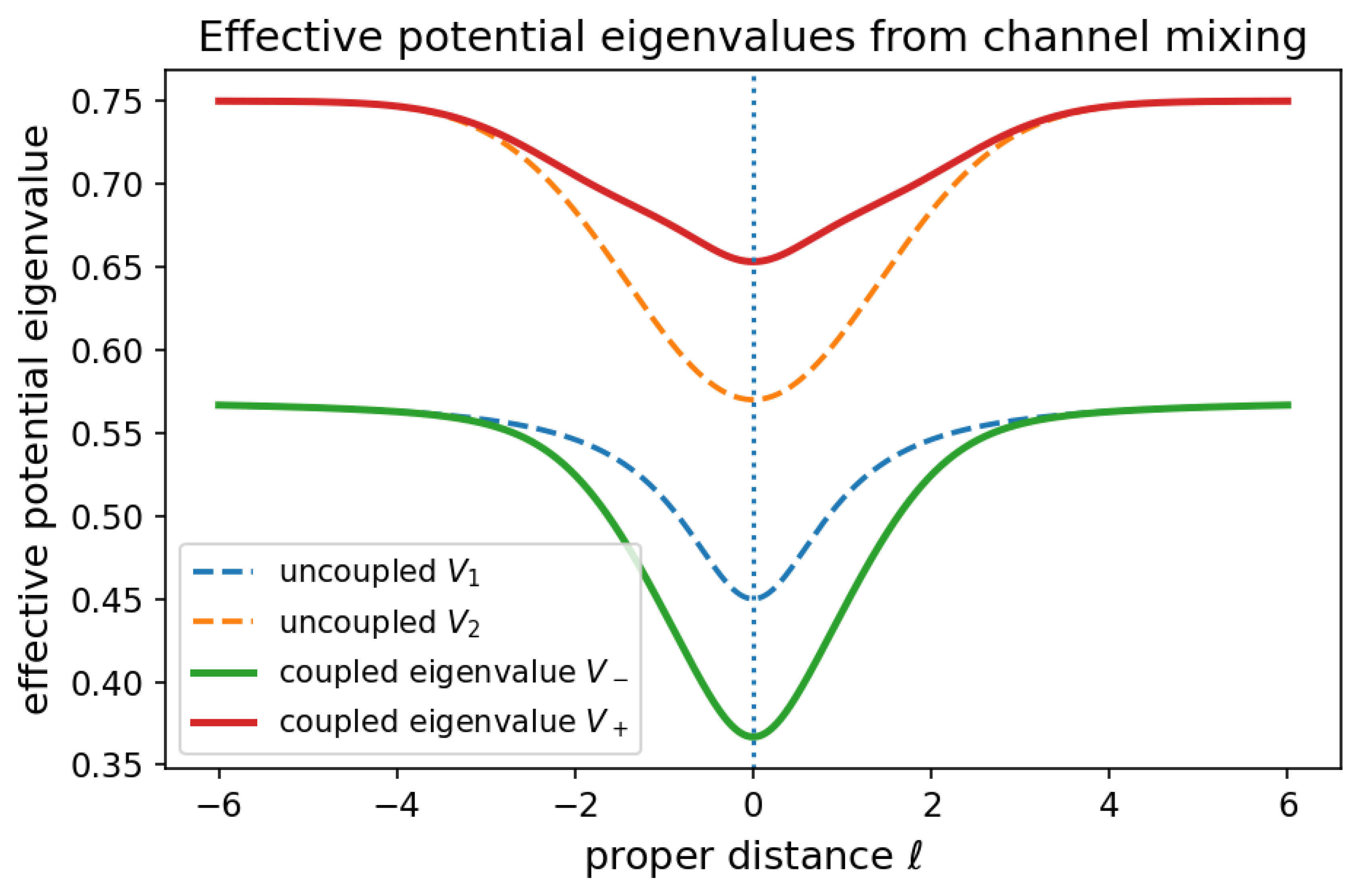
Figure 2.
Schematic avoided crossing in a two-channel spectral truncation of the coupled spectral problem. Dashed curves denote uncoupled channel frequencies, while solid curves show the coupled pole locations obtained from the eigenvalues of the effective spectral matrix or, equivalently, from the determinant condition . Angular-channel mixing converts isolated channel modes into collective normal modes of the coupled system and produces the characteristic spectral repulsion near the crossing point. The minimum spectral gap is controlled by the coupling strength through .
Figure 2.
Schematic avoided crossing in a two-channel spectral truncation of the coupled spectral problem. Dashed curves denote uncoupled channel frequencies, while solid curves show the coupled pole locations obtained from the eigenvalues of the effective spectral matrix or, equivalently, from the determinant condition . Angular-channel mixing converts isolated channel modes into collective normal modes of the coupled system and produces the characteristic spectral repulsion near the crossing point. The minimum spectral gap is controlled by the coupling strength through .
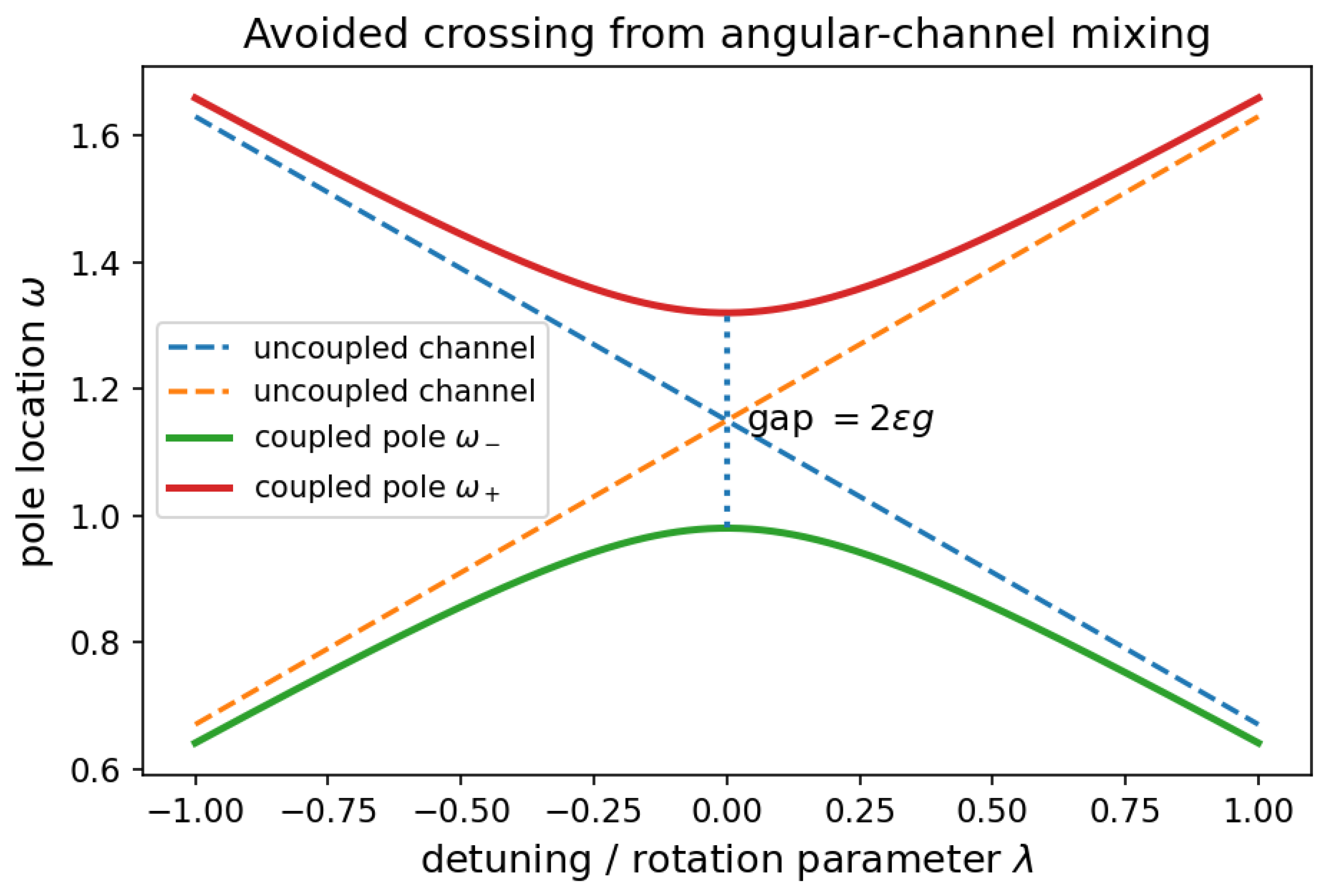
Figure 4.
Illustrative spectral response of the matrix-valued Green’s function for several values of the angular-channel coupling strength . The parameter is a small regulator used to display real normal-mode poles as finite Lorentzian peaks; it does not represent physical damping. The peaks correspond to coupled normal-mode poles of the effective matrix response function and provide a direct spectral signature of the underlying coupled-channel operator structure. As the coupling strength increases, the poles separate due to collective spectral repulsion induced by off-diagonal channel mixing. Because the rotating AdS-Teo wormhole defines a conservative self-adjoint spectral problem, the physical poles remain confined to the real frequency axis rather than moving into the complex plane as dissipative quasinormal modes.
Figure 4.
Illustrative spectral response of the matrix-valued Green’s function for several values of the angular-channel coupling strength . The parameter is a small regulator used to display real normal-mode poles as finite Lorentzian peaks; it does not represent physical damping. The peaks correspond to coupled normal-mode poles of the effective matrix response function and provide a direct spectral signature of the underlying coupled-channel operator structure. As the coupling strength increases, the poles separate due to collective spectral repulsion induced by off-diagonal channel mixing. Because the rotating AdS-Teo wormhole defines a conservative self-adjoint spectral problem, the physical poles remain confined to the real frequency axis rather than moving into the complex plane as dissipative quasinormal modes.
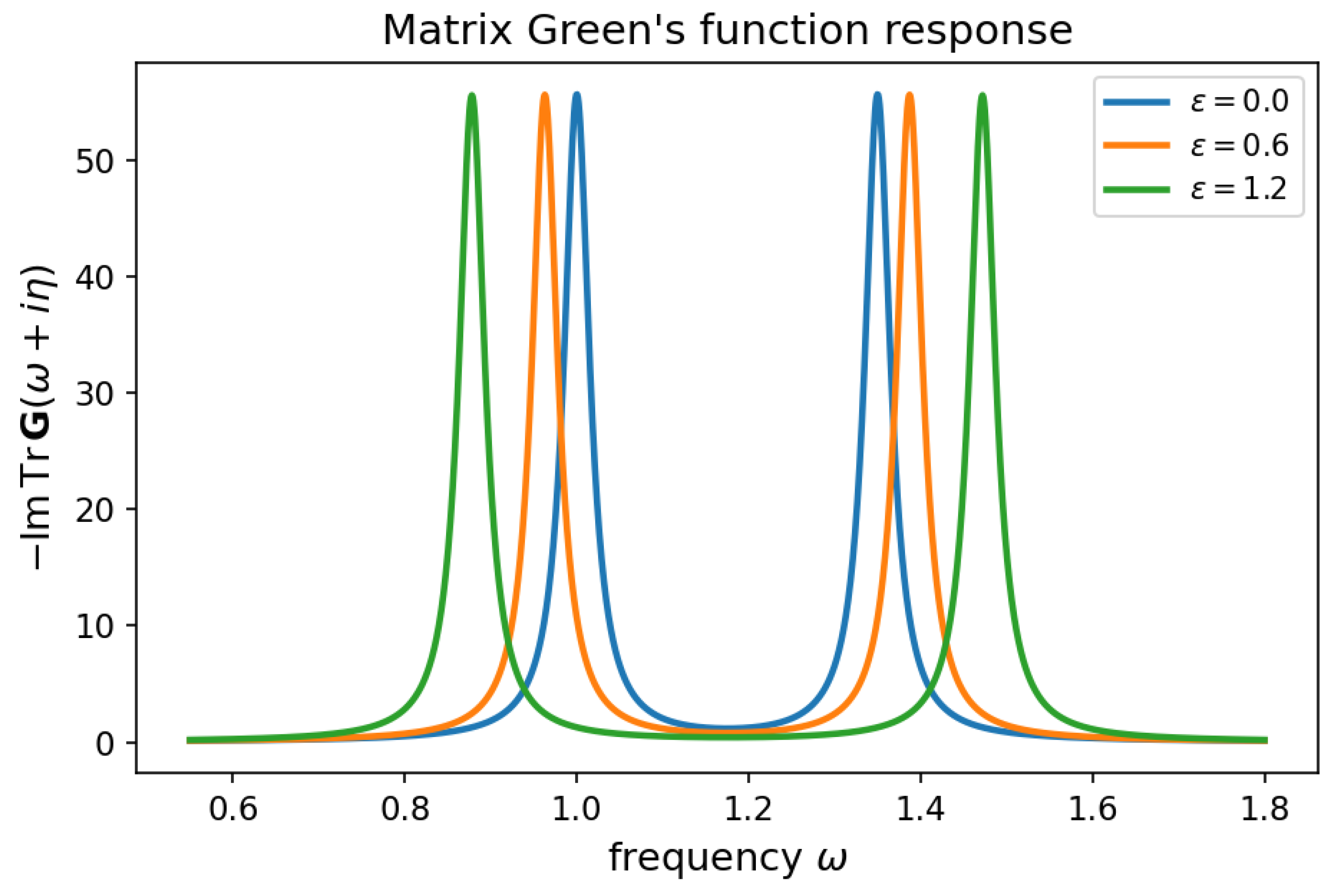
Figure 5.
Determinant response map for the illustrative two-channel spectral model, showing as a function of the real frequency and the coupling strength . The color scale represents the magnitude of the determinant-response diagnostic. Purple regions correspond to small response, while bright yellow ridges indicate regions where the determinant is close to zero and the coupled spectral response is strongly enhanced. The dashed white curves show the analytic pole trajectories obtained from Eq. (164). As the angular-channel coupling increases, the pole locations move continuously away from their uncoupled locations due to collective spectral repulsion while remaining confined to the real frequency axis. This reflects the conservative self-adjoint structure of the horizonless rotating wormhole geometry.
Figure 5.
Determinant response map for the illustrative two-channel spectral model, showing as a function of the real frequency and the coupling strength . The color scale represents the magnitude of the determinant-response diagnostic. Purple regions correspond to small response, while bright yellow ridges indicate regions where the determinant is close to zero and the coupled spectral response is strongly enhanced. The dashed white curves show the analytic pole trajectories obtained from Eq. (164). As the angular-channel coupling increases, the pole locations move continuously away from their uncoupled locations due to collective spectral repulsion while remaining confined to the real frequency axis. This reflects the conservative self-adjoint structure of the horizonless rotating wormhole geometry.
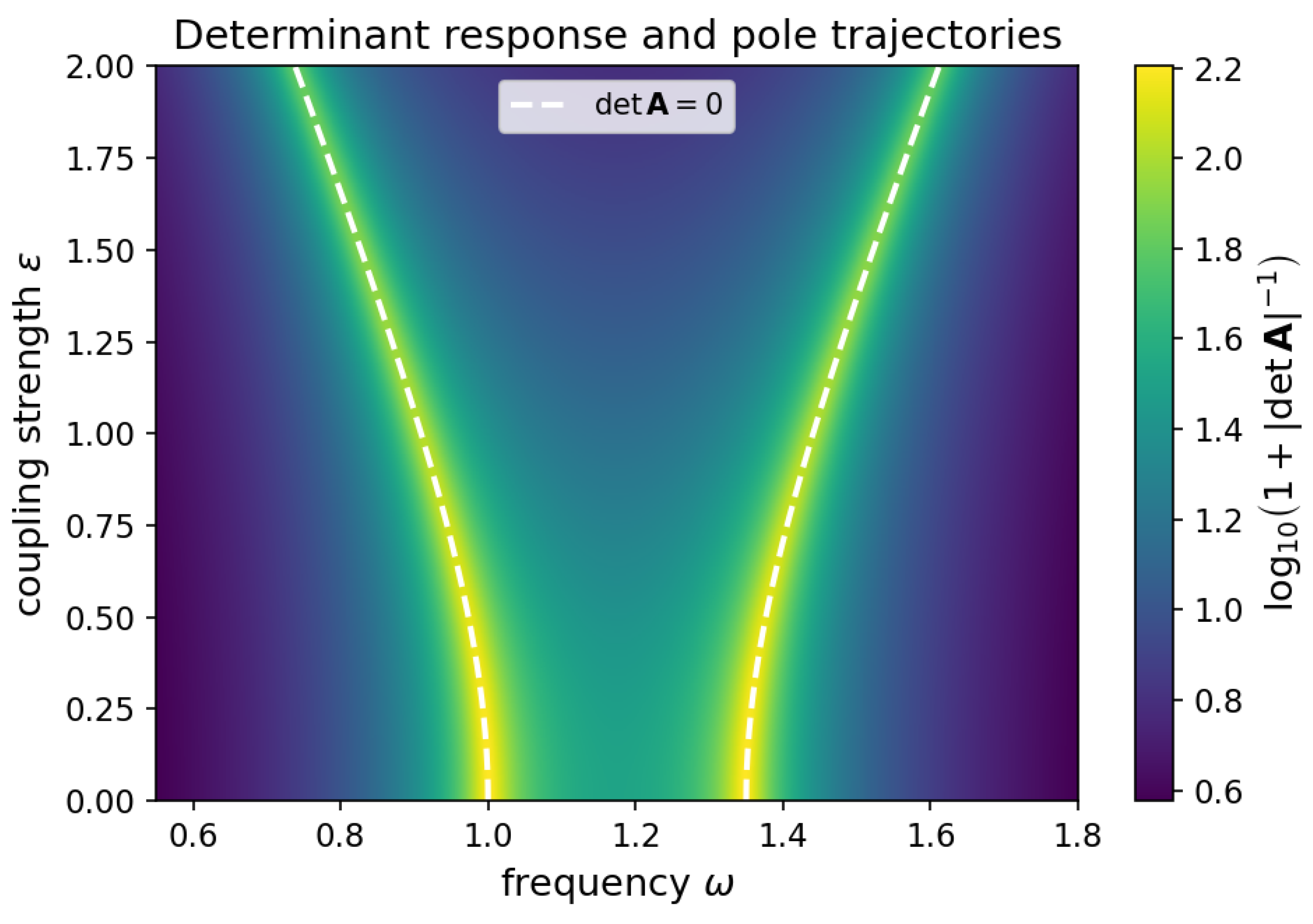
Figure 6.
Schematic illustration of the qualitative difference between the spectral organization of the rotating AdS-Teo wormhole and that of a dissipative black-hole-like system. The blue and orange points represent the lower and upper normal-mode branches of an illustrative coupled-channel wormhole model. As the channel coupling is increased, the two branches undergo coupling-induced level repulsion while remaining on the real frequency axis, reflecting the conservative self-adjoint character of the horizonless spectral problem. The dashed curves represent schematic black-hole-like quasinormal-mode branches displaced into the lower half of the complex frequency plane by damping. In contrast to the wormhole normal modes, quasinormal modes possess nonzero imaginary parts associated with decay and energy loss through horizon absorption. The figure is intended only as a conceptual visualization of the contrast between conservative normal-mode spectra and dissipative quasinormal-mode spectra and does not represent a numerical spectrum of either geometry.
Figure 6.
Schematic illustration of the qualitative difference between the spectral organization of the rotating AdS-Teo wormhole and that of a dissipative black-hole-like system. The blue and orange points represent the lower and upper normal-mode branches of an illustrative coupled-channel wormhole model. As the channel coupling is increased, the two branches undergo coupling-induced level repulsion while remaining on the real frequency axis, reflecting the conservative self-adjoint character of the horizonless spectral problem. The dashed curves represent schematic black-hole-like quasinormal-mode branches displaced into the lower half of the complex frequency plane by damping. In contrast to the wormhole normal modes, quasinormal modes possess nonzero imaginary parts associated with decay and energy loss through horizon absorption. The figure is intended only as a conceptual visualization of the contrast between conservative normal-mode spectra and dissipative quasinormal-mode spectra and does not represent a numerical spectrum of either geometry.
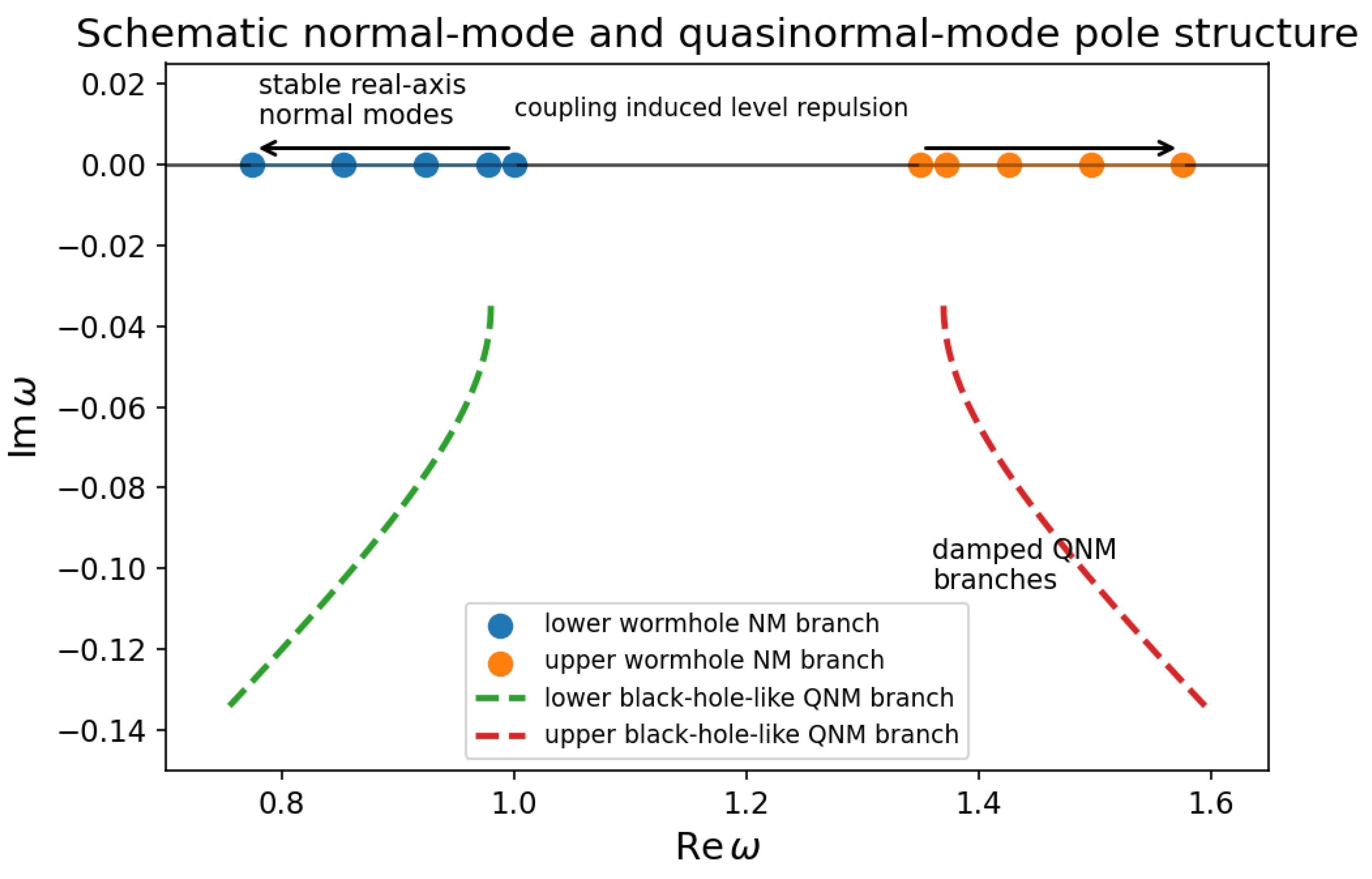
Figure 7.
Illustrative finite-mode vacuum-polarization profile near the wormhole throat for several values of the angular-channel coupling strength . The plotted curves model the finite coupled-channel contribution remaining after the universal Hadamard short-distance divergence has been subtracted. Diagonal channel terms provide the baseline profile, while off-diagonal interference between coupled angular channels generates localized oscillatory structure near . The figure is schematic and is not a full numerical Hadamard-renormalized computation in the complete rotating AdS-Teo geometry. The vertical dotted line marks the location of the wormhole throat.
Figure 7.
Illustrative finite-mode vacuum-polarization profile near the wormhole throat for several values of the angular-channel coupling strength . The plotted curves model the finite coupled-channel contribution remaining after the universal Hadamard short-distance divergence has been subtracted. Diagonal channel terms provide the baseline profile, while off-diagonal interference between coupled angular channels generates localized oscillatory structure near . The figure is schematic and is not a full numerical Hadamard-renormalized computation in the complete rotating AdS-Teo geometry. The vertical dotted line marks the location of the wormhole throat.
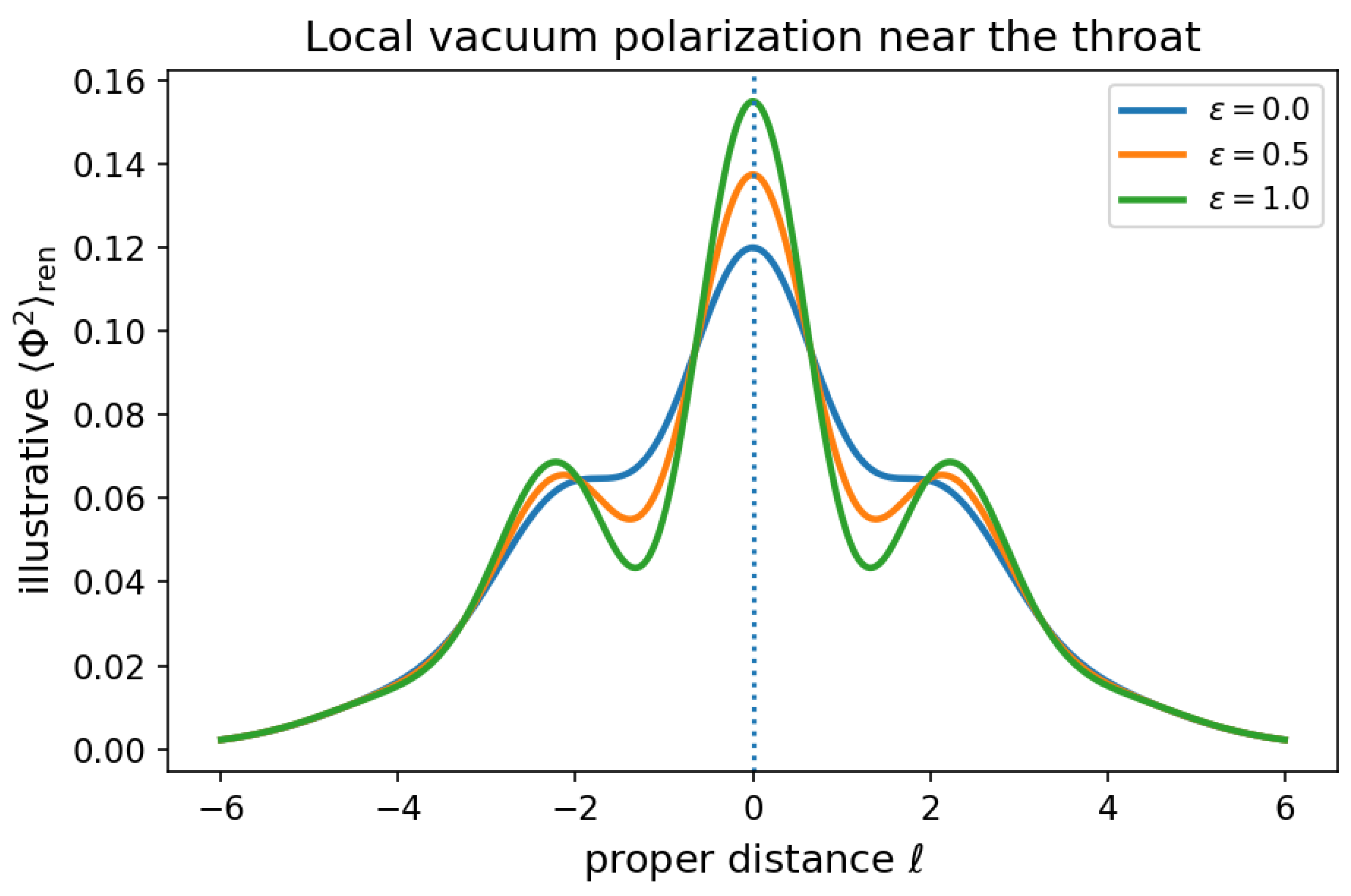
Disclaimer/Publisher’s Note: The statements, opinions and data contained in all publications are solely those of the individual author(s) and contributor(s) and not of MDPI and/or the editor(s). MDPI and/or the editor(s) disclaim responsibility for any injury to people or property resulting from any ideas, methods, instructions or products referred to in the content. |
© 2026 by the authors. Licensee MDPI, Basel, Switzerland. This article is an open access article distributed under the terms and conditions of the Creative Commons Attribution (CC BY) license.
Copyright: This open access article is published under a Creative Commons CC BY 4.0 license, which permit the free download, distribution, and reuse, provided that the author and preprint are cited in any reuse.


